Structure preserving integrators for solving linear quadratic optimal control problems with applications to describe the flight of a quadrotor

Abstract

We present structure preserving integrators for solving linear quadratic optimal control problems. This problem requires the numerical integration of matrix Riccati differential equations whose exact solution is a symmetric positive definite time-dependent matrix which controls the stability of the equation for the state. This property is not preserved, in general, by the numerical methods. We propose second order exponential methods based on the Magnus series expansion which unconditionally preserve positivity for this problem and analyze higher order Magnus integrators. This method can also be used for the integration of nonlinear problems if they are previously linearized. The performance of the algorithms is illustrated with the stabilization of a quadrotor which is an unmanned aerial vehicle.

1 Introduction

Nonlinear control problems have attracted the interest of researchers in different fields, e.g., the control of airplanes, helicopters, satellites, etc. [8, 11, 14] during the last years. While the extensively studied linear quadratic optimal control (LQ) problems can be used for solving simplified models, most realistic problems are inherently nonlinear. Furthermore, nonlinear control theory can improve the performance of the controller and enable tracking of aggressive trajectories [13].

Solving nonlinear optimal control problems requires the numerical integration of systems of coupled non-autonomous and nonlinear equations with boundary conditions for which it is of great interest to have simple, fast, accurate and reliable numerical algorithms for real time integrations.

It is usual to solve the nonlinear problems by linearization, which leads to problems that are solvable by linear quadratic methods.In general, they require the integration of matrix Riccati differential equations (RDEs) iteratively.The algebraic structure of the RDEs appearing in this problem implies that their solutions are symmetric positive definite matrices, a property that plays an important role for the qualitative and quantitative solutions of both the control and the state vector.

Geometric numerical integrators are numerical algorithms which preserve most of the qualitative properties of the exact solution. However, the mentioned positivity of the solution in this problem is a qualitative property which is not unconditionally preserved by most methods, geometric integrators included.

We show that some low order exponential integrators unconditionally preserve this property, and higher order methods preserve it under mild constraints on the time step. We refer to these methods as structure preserving integrators, and they will allow the use of relatively large time steps while showing a high performance for stiff problems or problems which strongly vary along the time evolution.

The aforementioned nonlinearities in the control problems can be dealt with in different ways. We consider three techniques to linearize the equations and the linear equations are then numerically solved using some exponential integrators which preserve the relevant properties of the solution. Since the nonlinear problems are solved by linearization, we first examine the linear problem in detail.

The paper is organized as follows: The linear case is studied in Section 2, where we emphasize on the algebraic structure of the equations and the qualitative properties of the solutions. We next consider some exponential integrators and analyze the preservation of the qualitative properties of the solution by the proposed methods. In Section 3, it is shown how the full nonlinear problem can - after linearization - be treated as a particular case of the non-autonomous linear one. The work concludes with the application of the numerical algorithm to a particular example (control of a quadrotor) in Section 4, with which the accuracy of the exponential methods is demonstrated. Numerical results and conclusions are included.

2 Linear quadratic (LQ) methods in optimal control problems

Let us consider the general LQ optimal control problem

$$\min_{u\in L^{2}}\int_{0}^{t_{f}}\left(X^{T}(t)Q(t)X(t)+u^{T}(t)R(t)u(t)\right)\,dt$$ (1a)

$$\text{subject to}\quad\dot{X}(t)=A(t)X(t)+B(t)u(t),\quad X(0)=X_{0},$$ (1b)

where $\dot{X}(t)$ is the time-derivative of the state vector $X(t)\in\mathbb{R}^{n}$, $u(t)\in\mathbb{R}^{m}$ is the control, $R(t)\in\mathbb{R}^{m\times m}$ is symmetric and positive definite, $Q(t)\in\mathbb{R}^{n\times n}$ is symmetric positive semi-definite, $A\in\mathbb{R}^{n\times n},B\in\mathbb{R}^{n\times m}$ and $M^{T}$ denotes the transpose of a matrix $M$.

Problems of the type (1) are frequent in many areas, such as game theory, quantum mechanics, economy, environment problems, etc., see [6, 18], or in engineering models [2, ch. 5].

The optimal control problem (1) is solved, assuming some controllability conditions, by the linear feedback controller [21]

$$u(t)=-K(t)X(t),$$ (2)

with the gain matrix

$$K(t)\,=\,R^{-1}(t)B^{T}(t)P(t)\,,$$

and $P(t)$ verifying the matrix RDE

$$\dot{P}(t)=-P(t)A(t)-A^{T}(t)P(t)+P(t)B(t)R^{-1}(t)B^{T}(t)P(t)-Q(t),$$ (3)

with the final condition $P(t_{f})=0$. The solution $P(t)$ after backward time integration of (3) is a symmetric and positive definite matrix when both $Q(t)$ and $R(t)$ are symmetric positive definite [1] (similar results also apply for the weaker condition $Q(t)$ positive semidefinite under general conditions on the matrices which make the system stabilizable and detectable). To compute the optimal control $u(t)$, we solve for $P(t)$, and plugging the control law into (1b) yields a linear equation for the state vector

$$\dot{X}(t)=\left(A(t)-B(t)R^{-1}(t)B^{T}(t)P(t)\right)X(t),\quad X(0)=X_{0},$$

to be integrated forward in time, with which the control is readily computed. Notice that $S(t)=B(t)R^{-1}(t)B^{T}(t)$ is a positive semi-definite symmetric matrix (positive definite if $\ rank\,B=n$) and $P(t)$ is a positive definite matrix, hence its product is also a positive semi-definite matrix, and this is very important for the stability of the solution for the state vector and ultimately for the control. A numerical integrator which does not preserve the positivity of $P(t)$ can become unstable when solving the state vector.

In this paper, exponential integrators, which belong to the class of Lie group methods (see [7, 19] and references therein), are proposed in order to solve the RDE (3). They are geometric integrators because they preserve some of the qualitative properties of the exact solution.

2.1 Structure preserving integrators

We are interested in numerical integrators which preserve the symmetry as well as the positivity of $P(t)$. While symmetry is a property preserved by most methods, the preservation of positivity is a more challenging task.

For our analysis, it is convenient to review some results from the numerical integration of differential equations. Given the ordinary differential equation (ODE)

$$\dot{x}=f(x,t),\qquad x(t_{0})=x_{0}\in\mathbb{R}^{n},$$ (4)

the exact solution at time $t=t_{0}+h$ can formally be written as a map that takes initial conditions to solutions, $\Phi_{h}(x_{0})=x(t_{0}+h)$. For sufficiently small $h$, it can also be interpreted as the exact solution at time $t=t_{0}+h$ of an autonomous ODE

$$\dot{x}=f_{h}(x),\qquad x(t_{0})=x_{0},$$

where $f_{h}$ is the vector field associated to the Lie operator $\ \frac{1}{h}\log(\Phi_{h})$.

In a similar way, a numerical integrator for solving the equation (4) which is used with a time step $h$, can be seen as the exact solution at time $t=t_{0}+h$ of a perturbed problem (backward error analysis)

$$\dot{x}=\tilde{f}_{h}(x),\qquad x(t_{0})=x_{0},$$

and we say that the method is of order $p$ if $\tilde{f}_{h}-f_{h}=\mathcal{O}(h^{p+1})$. The qualitative properties of the exact solution $\Phi_{h}$ are related to the algebraic structure of the vector field $f_{h}$: If the vector field $\tilde{f}_{h}$ associated with the numerical integrator shares the same algebraic structure, the numerical integrator will preserve these qualitative properties.

Given the RDE

$$\dot{P}=PA(t)+A^{T}(t)P-PS(t)P+Q(t),\qquad P(t_{0})=0,$$

which is equivalent to (3) with the sign of the time changed, i.e., integrated backward in time, and with $Q(t),S(t)$ symmetric and positive definite matrices, then $P(t)$, for $t>t_{0}$, is also a symmetric and positive definite matrix. Thus, a numerical integrator which can be considered as the exact solution of a perturbed matrix RDE

$$\dot{P}=P\tilde{A}_{h}+\tilde{A}^{T}_{h}P-P\tilde{S}_{h}P+\tilde{Q}_{h},\qquad P(t_{0})=0,$$

where $\tilde{Q}_{h},\tilde{S}_{h}$ are symmetric positive definite matrices will preserve the symmetry and positivity of the exact solution. The same result applies if the numerical integrator is given by a composition of maps such that each one, separately, can be seen as the exact solution of a matrix RDE with the same structure.

We will refer to these methods as positivity preserving integrators. If a method preserves positivity for all $h>0$, we say it is unconditionally positivity preserving and, if there exists $h^{*}>0$ such that this property is preserved for $0<h<h^{*}$, we will refer to it as conditionally positive preserving.

In general, standard methods do not preserve positivity. We show, however, that some second order exponential integrators preserve positivity unconditionally and higher order ones are conditionally positivity preserving for a relatively large range of values of $h^{*}$ which depends on the smoothness in the time dependence of the matrices $A(t),S(t),Q(t)$. At this stage, it is convenient to rewrite the RDE (3) as a linear differential equation

$$\frac{d}{dt}\begin{bmatrix}V(t)\\ W(t)\end{bmatrix}=\begin{bmatrix}-A(t)^{T}&-Q(t)\\ -S(t)&A(t)\end{bmatrix}\,\begin{bmatrix}V(t)\\ W(t)\end{bmatrix},\quad\begin{bmatrix}V(t_{f})\\ W(t_{f})\end{bmatrix}=\begin{bmatrix}P_{f}\\ I\end{bmatrix},$$ (5)

where $P_{f}=0$, $S(t)=B(t)R^{-1}(t)B^{T}(t)$ and the solution $P(t)$ of problem (3), to be integrated backward in time, is given by

$$P(t)=V(t)W(t)^{-1},\quad P(t),V(t),W(t)\in\mathbb{R}^{n\times n},$$

in the region where $W(t)$ is invertible (see, for instance, [7] or [20], and references therein). If $R(t)$ and $Q(t)$ are positive definite matrices, this problem always has a solution.

It is then clear that if a numerical integrator for the equation (5) can be regarded as the exact solution of an autonomous perturbed linear equation

$$\frac{d}{dt}\begin{bmatrix}V(t)\\ W(t)\end{bmatrix}=\begin{bmatrix}-\tilde{A}_{h}^{T}&-\tilde{Q}_{h}\\ -\tilde{S}_{h}&\tilde{A}_{h}\end{bmatrix}\,\begin{bmatrix}V(t)\\ W(t)\end{bmatrix},\quad\begin{bmatrix}V(t_{f})\\ W(t_{f})\end{bmatrix}=\begin{bmatrix}P_{f}\\ I\end{bmatrix},$$

where $\tilde{Q}_{h}$ and $\tilde{S}_{h}$ are symmetric and positive definite matrices, then the numerical solution is symmetric and positive definite.

In general, high order standard methods like Runge-Kutta methods do not preserve positivity. Explicit methods applied to the linear problem do not preserve positivity unconditionally, but to show this result for implicit methods requires a more detailed analysis and it is stated in the following theorem.

Theorem 2.1

The second order implicit midpoint and trapezoidal Runge-Kutta methods do not preserve positivity unconditionally for the solution of the RDE (5).

Proof 2.2

It suffices to prove it for the scalar non-autonomous problem

$$\dot{p}=-q-2a(t)\,p+s\,p^{2},\qquad\quad p(t_{f})=0$$ (6)

with $q,s>0$ and $a:[0,t_{f}]\to\mathbb{R}$. Let $a(t)=0$ for $t\in[t_{f}-h,t_{f}]$ and $a(t)=a<0$ for $t\in[0,t_{f}-3h/2]$. Then, for the implicit midpoint rule, two iterations backwards in time starting with $p_{0}=0$ yield a negative value $p_{2}<0$ if $|a|>2/h$. For the trapezoidal rule, three iterations are necessary to reach negative values, with a sufficient condition for $p_{3}<0$ being

$$a<-\frac{3}{h}+hq\left(-\frac{1}{4}+\frac{6}{-4+h^{2}q}\right)\quad\wedge\quad h<\frac{2}{\sqrt{q}}.$$

We remark, that, given $a<0$, the method produces negative values $p_{3}$ for a range of time-steps, i.e., for larger time-steps $h$, it is less prone to negativity. Furthermore, not only can the methods produce negative values $p_{k}$, for certain parameter ranges they also attain complex valued results.

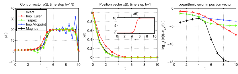
Figure 1: (color online) Exact and numerical solutions for the problem (6) with parameters given in (7) and using the implicit Euler, trapezoidal and midpoint Runge-Kutta methods as well as the second order Magnus integrator.

To better illustrate the results, we consider the problem (6) for

$$q=s=1,\qquad a(t)=\frac{10}{1+\exp(-4(t-t_{f}/2))},\qquad t_{f}=10,$$ (7)

with $h=1/2$ for the equation of $p(t)$ and $h=1$ for the equation of $x(t)$,

$$\dot{x}=\left(a\left(t\right)-sp\left(t\right)\right)x,\qquad x(0)=0.$$

We integrated the problem using the second order implicit trapezoidal and midpoint methods as well as the first order implicit Euler method. The results are shown in Figure 1, where we appreciate that the first order implicit Euler method is superior (the results obtained with the second order Magnus integrator to be presented in the next section is also included). The poor performance and non-positivity of the higher order standard implicit methods is manifest.

If we are interested in high order numerical integrators, different classes of methods have to be explored. We consider a particular class of exponential integrators referred to as Magnus integrators (see [4] and references therein).

2.2 Magnus integrators

Given the general linear equation

$$y^{\prime}=M(t)\,y\,,\qquad\quad y(t_{0})=y_{0}\,,$$ (8)

with $y\in\mathbb{R}^{p}$, and if we denote the fundamental solution by $\Phi(t,t_{0})\in\mathbb{R}^{p\times p}$, such that $y(t)=\Phi(t,t_{0})y(t_{0}),$ the Magnus expansion gives us the formal solution (under certain convergence conditions, see [4] and references therein) as

$$\Phi(t,t_{0})=\exp\left(\Omega(t,t_{0})\right),$$

where $\Omega(t,t_{0})=\sum_{n=1}^{\infty}\Omega_{n}(t,t_{0})$ and each $\Omega_{n}(t,t_{0})$ is an element of the Lie algebra generated by $n$-dimensional integrals involving $n-1$ nested commutators of $M(t)$ at different instants of time. The first two terms are given by

$$\Omega_{1}(t,t_{0})=\int_{t_{0}}^{t}M(s)\,ds,\qquad\Omega_{2}(t,t_{0})=\frac{1}{2}\int_{t_{0}}^{t}\,dt_{1}\int_{t_{0}}^{t_{1}}[M(t_{1}),M(t_{2})]\,dt_{2},$$

where $[A,B]=AB-BA$.

In the region of convergence of the Magnus expansion, the exact solution at time $t=t_{0}+h$ is equivalent to the exact solution of the autonomous linear equation

$$y^{\prime}=\frac{1}{h}\Omega(t_{0}+h,t_{0})\,y\,,\qquad\quad y(t_{0})=y_{0}\,.$$

It is well known that the set of matrices

$$\left[\begin{array}[]{cc}A&B\\ C&-A^{T}\end{array}\right],$$ (9)

with $A,B,C\in\mathbb{R}^{n\times n}$ and $B=B^{T},\ C=C^{T}$ form the algebra of symplectic matrices. This algebraic property is preserved by the commutators and then any truncated Magnus expansion preserves symplecticity for this problem. However, the additional property about the positivity (or negativity) of the skew diagonal matrices $B,C$ is not always guaranteed when the series is truncated. We analyze lower order methods and show that it is possible to build second order Magnus integrators which unconditionally preserve positivity.

The first term in the expansion applied to (5) does not contain commutators and is given by

$$\Omega_{1}(t,t_{0})=\begin{bmatrix}\displaystyle-\int_{t_{0}}^{t}A(s)^{T}\,ds&\displaystyle-\int_{t_{0}}^{t}Q(s)\,ds\\ &\\ \displaystyle-\int_{t_{0}}^{t}S(s)\,ds&\displaystyle\int_{t_{0}}^{t}A(s)\,ds\end{bmatrix}\,.$$ (10)

Then, if we truncate the series after the first term and approximate the integrals for a time interval $t\in[t_{0},t_{0}+h]$ using a quadrature rule of second or higher order, we obtain a second order method.

It is well known that, if $Q(t)$ is a symmetric positive definite matrix for $t\in[t_{0},t_{0}+h]$, then $\ \hat{Q}_{h}=\int_{t_{0}}^{t_{0}+h}Q(s)\,ds\$ is also symmetric positive definite. Suppose now that the integral is approximated using a quadrature rule

$$\tilde{Q}_{h}\equiv h\sum_{i=1}^{k}b_{i}Q(t_{0}+c_{i}h)\simeq\int_{t_{0}}^{t_{0}+h}Q(s)\,ds,$$

with $\ c_{i}\in[0,1],\ i=1,\ldots,k$. If $\ \sum_{i}b_{i}>0\,$, we have:

a)

If $b_{i}>0,\ i=1,\ldots,k$, then $\tilde{Q}_{h}$ is a symmetric positive definite matrix.

b)

If $\exists\,b_{j}<0,\$ for some value of $j$ and $\|Q(t_{m})-Q(t_{n})\|<C|t_{m}-t_{n}|,\ \forall t_{m},t_{n}\in[t_{0},t_{0}+h]$, then $\exists\ h^{*}>0$ such that $\tilde{Q}_{h}$ is a symmetric positive definite matrix for $0<h<h^{*}$, and $h^{*}$ depends on $C$.

The same results also apply to $\tilde{S}_{h}$.

A second order method which preserves positivity is constructed by taking the first term in the Magnus expansion (10) and approximating the integrals by a second or higher order rule with the constraint that all $b_{i}>0$. The most natural choices are the midpoint rule

$$\Psi_{h}^{[2]}=\exp\left(hM(t+h/2)\right)=\Phi(t+h,t)+\mathcal{O}(h^{3}),$$

or the trapezoidal rule

$$\Psi_{h}^{[2]}=\exp\left(\frac{h}{2}\left[M(t+h)+M(t)\right]\right)=\Phi(t+h,t)+\mathcal{O}(h^{3}).$$ (11)

The latter of which is found more efficient since less evaluations of the functions in the algorithm are necessary as they can be reused in the computation of $X(t)$. If we consider the RDE (3) that corresponds to (8) with the data (5) and choose an equidistant time grid $t_{n}=t_{0}+nh\,$, $\ 0\leq n\leq N\,$, with constant time step $\,h=(t_{f}-t_{0})/N\,$ and taking into account that this equation has to be solved backward in time, we obtain

$$\left[\begin{array}[]{c}V_{n}\\ W_{n}\end{array}\right]=\exp\left(-\frac{h}{2}\left[M(t_{n})+M(t_{n+1})\right]\right)\left[\begin{array}[]{c}V_{n+1}\\ W_{n+1}\end{array}\right]\ \Rightarrow\ \tilde{P}_{n}=V_{n}\,W_{n}^{-1}\,,$$

By construction, $\tilde{P}_{n}$ is a symmetric positive definite matrix. In addition, it is also a time symmetric second order approximation to $P(t_{n})$. In this way, the matrix functions $A(t_{n})$, $B(t_{n})$, $Q(t_{n})$, $R(t_{n})$ are computed at the same mesh points as the approximations $\tilde{P}_{h}$ of $P(t)$ and, as we will see, they can be reused for the forward time integration of the state vector.

Let us consider the equation for the state vector, to be integrated forward in time, which takes the form

$$\dot{X}=(A(t)-S(t)\tilde{P}_{h})X,$$

where we denote by $\tilde{P}_{h}$ the numerical approximations to $P(t)$ computed on the mesh and $\tilde{P}_{h,n}\simeq P(t_{n})$. Notice that at the instant $t=t_{f}-h$, we have that $\tilde{P}_{h,N-1}=P(t_{f}-h)+\mathcal{O}(h^{3})$ (local error) but at $t=t_{0}$, after $N$ steps, we have $\tilde{P}_{h,0}=P(t_{0})+\mathcal{O}(h^{2})$ (global error). This accuracy suffices to get a second order approximation for the numerical approximation to the state vector.

If we use the same Magnus expansion for the numerical integration of the state vector with the trapezoidal rule, we have the algorithm

$$X_{n+1}=\exp\left(\frac{h}{2}\left[D_{n+1}+D_{n}\right]\right)\,X_{n}\,,\ \quad D_{m}=A_{m}-S_{m}\tilde{P}_{h,m},\quad m=n,n+1,$$

where $A_{m}=A(t_{m})$, $S_{m}=S(t_{m})$.

Finally, the controls which allow us to reach the final state in a nearly optimal way are computed via

$$u_{n}\,=\,-R^{-1}(t_{n})B^{T}(t_{n})P_{n}\,X_{n}\,.$$

Higher order Magnus integrators

Truncating the Magnus expansion at higher powers of $h$ usually requires the computation of matrix commutators. If we include, for example, the second term $\Omega_{2}$ in the exponent, we obtain $\Psi_{h}\equiv\exp\left(\Omega_{1}+\Omega_{2}\right)$, which agrees with the exact solution up to order four, i.e., $\Psi_{h}=\Phi(t+h,t)+\mathcal{O}(h^{5})$. The sum $\Omega_{1}+\Omega_{2}$ belongs to the algebra of symplectic matrices, as given in (9), where the off-diagonal matrices $B,C$ take an involved form. We will show that positivity is conditionally preserved, however, unconditional preservation as for $\exp\left(\Omega_{1}\right)$ cannot be achieved.

For simplicity in the analysis, we consider commutator-free Magnus integrators (see [4, 5] and references therein). With the abbreviations

$$M^{(0)}=\int_{t_{n}}^{t_{n}+h}M(s)\,ds,\qquad M^{(1)}=\frac{1}{h}\int_{t_{n}}^{t_{n}+h}\left(s-\left(t_{n}+\frac{h}{2}\right)\right)M(s)\,ds,$$

the following commutator-free composition gives an approximation to fourth-order

$$\Psi_{CF}^{[4]}=\exp\left(\frac{1}{2}M^{(0)}+2M^{(1)}\right)\,\exp\left(\frac{1}{2}M^{(0)}-2M^{(1)}\right)=\Phi(t_{0}+h,t_{0})+\mathcal{O}(h^{5}).$$

Using the fourth-order Gaussian quadrature rule to approximate the integrals yields

$$\Psi_{G}^{[4]}=\exp\left(h(\beta M_{1}+\alpha M_{2})\right)\exp\left(h(\alpha M_{1}+\beta M_{2})\right),$$

where $M_{i}\equiv M(t_{n}+c_{i}h),\ i=1,2$, $c_{1}=\frac{1}{2}-\frac{\sqrt{3}}{6},\ c_{2}=\frac{1}{2}+\frac{\sqrt{3}}{6}$, $\alpha=\frac{1}{4}-\frac{\sqrt{3}}{6}=-0.038\ldots<0,\ \beta=\frac{1}{4}+\frac{\sqrt{3}}{6}$. This composition will not preserve positivity unconditionally when applied to solve the RDE because $\alpha<0$. However, since $\alpha+\beta=\frac{1}{2}$ the positivity will be conditionally preserved.

If we approximate the integrals using the Simpson rule, we have

$$\Psi_{G}^{[4]}=\exp\left(\frac{h}{12}(-M_{1}+4M_{2}+3M_{3})\right)\exp\left(\frac{h}{12}(3M_{1}+4M_{2}-M_{3})\right),$$

where $M_{1}\equiv M(t_{n}),M_{2}\equiv M(t_{n}+h/2),M_{3}\equiv M(t_{n}+h)$. As previously, one of the coefficients is negative and positivity is not unconditionally preserved when the method is applied to the RDE.

Recall that the full problem requires the solution of two differential equations; suppose we want to (backward) integrate the matrix RDE with one of the fourth-order commutator-free methods and then use the same method for the (forward) integration of the state vector, we need to use a time step twice as large for the forward integration (preferably with the Simpson rule, since no interpolation is necessary).

The main goal of this paper is to present a simple, fast, accurate and reliable numerical scheme for nonlinear problems. As we will see, nonlinear problems are linearized, and the resulting linear equations are solved iteratively. The solution of each iteration is plugged into the following iteration, and this requires to use a fixed mesh for all methods. For this reason, the second order Magnus integrator is the optimal candidate among the previous and is used in the numerical examples in section 4.

3 The nonlinear control problem

Many problems in engineering can be stated as optimal control problems of the form

$$\underset{u\in L^{2}}{\min}\int_{0}^{t_{f}}\left(X^{T}(t)Q(t,X(t))X(t)+u^{T}(t)R(t,X(t))u(t)\right)\,dt$$ (12a)

$$\text{subject to}\quad\dot{X}(t)=f_{A}\left(t,X\left(t\right)\right)+f_{B}\left(t,X\left(t\right),u\left(t\right)\right),\quad X(0)=X_{0}.$$ (12b)

This nonlinear optimal control problem is considerably more involved than its linear counterpart. It is then usual to solve the nonlinear problem by linearization, and this can be done in different ways. In the following, under the assumption that $f_{B}$ depends linearly on $u$, we present three of them and compare their performances when the linear equations are solved using exponential integrators.

Quasilinearization

For $f_{A}(t,0)=0$ and $f_{B}(t,X,u)\neq 0$ for all $t,X$ in the appropriate domains, the state equation (12b) can be written in a non-unique way as

$$\dot{X}(t)=A(t,X)X(t)+B(t,X)u(t),\quad X(0)=X_{0}.$$ (13)

The formulation (13) is the basic ingredient for the State Dependent Riccati Equation (SDRE) control technique [15, 16]. Its formal similarity to the linear problem (1) motivates the imitation of the optimal LQ controller by defining

$$u(t)=-R^{-1}(t)B^{T}(t,X(t))P(t,X)X(t)$$ (14a)

where $$P(t,X)$$ solves the now state-dependent algebraic Riccati equation

$$0=-PA(t,X)-A(t,X)^{T}P+PB(t,X)R(t,X)^{-1}B(t,X)^{T}P-Q(t,X).$$ (14b)

One has to choose the unique positive definite solution of the algebraic Riccati equation and, combining (14a) with (13), the closed-loop nonlinear dynamics are given by

$$\dot{X}=\left(A(t,X)-B(t,X)R(t,X)^{-1}B(t,X)^{T}P(t,X)\right)X,\quad X(0)=X_{0}.$$ (14c)

The usual approach is to start from $X(0)=X_{0}$, and then to advance step by step in time by first computing $P$ from (14b) at each step and then applying the Forward Euler method on (14c). The application of higher order methods, such as Runge-Kutta schemes, requires to solve implicit systems with (14b) and can thus be costly. In addition, if one is interested in aggressive trajectories, the algebraic equation (14b) can considerably differ from the solution of the corresponding Riccati differential equation, which affects the solution of the state vector, $X$, and ultimately the control in (14a).

Waveform relaxation

Alternatively, we can linearize (14c), by iterating

$$\frac{d}{dt}X^{n+1}=\left(A(t,X^{n})-B(t,X^{n})R(t,X^{n})^{-1}B(t,X^{n})^{T}P(t,X^{n})\right)X^{n+1}.$$ (15)

We start with a guess solution $X^{0}(t)$ and iteratively obtain a sequence of solutions, $X^{1}(t)$, $X^{2}(t),\ldots,X^{n}(t)$. Again, the iteration stops once consecutive solutions differ by less than a given tolerance. Here, $P(t,X^{n}(t))$ at each iteration is obtained from

$$\dot{P}=-PA^{n}(t)-A^{n}(t)^{T}P+PB^{n}(t)R^{n}(t)^{-1}B^{n}(t)^{T}P-Q^{n}(t),\quad P(t_{f})=0,$$ (16)

with $A^{n}(t)\equiv A(t,X^{n}(t))$, $B^{n}(t)\equiv B(t,X^{n}(t))$, etc.

This procedure is similar to what is known as waveform relaxation [24], however, the backward integration for $P$ limits the parallelizability in this application. This approach corresponds to freezing the nonlinear parts in (13) at the previous state and then applying the optimal control law (2). It is worth noting that this technique can handle inhomogeneities by slightly adapting the control law, at the cost of solving an inhomogeneous linear system, see below. The algorithms are illustrated in Table 1.

A1: waveform relaxation

A2: linearization

$\begin{array}[]{l}n:=0;\quad\textit{guess}:X^{0}(t),u^{0}(t)\\ {\bf do}\\ \quad n:=n+1\\ \quad\text{compute}:A^{n-1}(t),B^{n-1}(t)\\ \quad\text{solve}\,(t_{f}\to 0):\text{eq. }\eqref{eq:rde}\textit{ for }P^{n-1}\\ \quad\text{solve}\,(0\to t_{f}):\text{eq. }\eqref{eq:x:mixed:iteration}\textit{ for }X^{n}\\ {\bf while}\ |X^{n}-X^{n-1}|>tolerance\\[2.84526pt] \textit{Check for feasibility of }X^{n}\\ \\ \end{array}$

$\begin{array}[]{l}n:=0;\quad\textit{guess}:X^{0}(t),u^{0}(t)\\ {\bf do}\\ \quad n:=n+1\\ \quad\text{compute}:\bar{A}^{n-1}(t),\bar{B}^{n-1}(t),\bar{C}^{n-1}(t)\\ \quad\text{solve}\,(t_{f}\to 0):\text{eq. }\eqref{eq:RDE}\textit{ for }P^{n-1}\\ \quad\text{solve}\,(t_{f}\to 0):\text{eq. }\eqref{eq:disturbance}\textit{ for }V^{n}\\ \quad\text{solve}\,(0\to t_{f}):\text{eq. }\eqref{eq:linearized:inhomogeneous}\textit{ for }X^{n}\\ {\bf while}\ |X^{n}-X^{n-1}|>tolerance\\[2.84526pt] \textit{Check for feasibility of }X^{n}\\ \end{array}$

Table 1: Algorithm (A1) for the waveform relaxation and algorithm (A2) for the Taylor-type linearization.

Taylor-type linearization

Similarly to [22], we can Taylor-expand the vector field in (12b) around an approximate solution $X^{n}(t)$ and use optimal LQ controls for the approximated equation. The iteration step reads then

$$\dot{X}^{n+1}(t)=\bar{A}^{n}(t)X^{n+1}(t)+\bar{B}^{n}(t)u^{n+1}(t)+\bar{C}^{n}(t),$$ (17)

where

$$\begin{array}[]{rl}\bar{A}^{n}(t)&=D_{X}f_{A}\left(t,X^{n}(t)\right)+D_{X}f_{B}\left(t,X^{n}(t),u^{n}(t)\right),\\ \bar{B}^{n}(t)&=D_{U}f_{B}(t,X^{n},U^{n}),\\ \bar{C}^{n}(t)&=f_{A}(t,X^{n})+f_{B}(t,X^{n},u^{n})-\left(\bar{A}^{n}(t)\cdot X^{n}+\bar{B}^{n}(t)\cdot u^{n}\right),\end{array}$$

and $D_{X}$ denotes the derivative with respect to $X$, etc. One starts with an initial guess, $X^{0}(t)$ and the iteration stops once consecutive iterations differ by less than a given tolerance.

The inhomogeneity $\bar{C}^{n}$ can be treated as a disturbance input and compensated by the controller [10]. The optimal control then becomes

$$u^{n+1}(t)=-{R^{n}(t)}^{-1}{\bar{B}^{n}(t)}^{T}\left(P^{n}(t)X^{n+1}(t)+V^{n}(t)\right)$$

where $P^{n}(t)$ satisfies (3) with replacements $A\to\bar{A}^{n}$ and $B\to\bar{B}^{n}$, etc. and $V^{n}(t)$ is given by

$$\dot{V} =\left(P\bar{B}R^{-1}{\bar{B}}^{T}-{\bar{A}}^{T}\right)V-P\bar{C},\quad V(t_{f})=0$$ (18)

at each iteration. The linearization procedure is summarized in Table 1.

NOTE: We can solve non-homogeneous equations with Magnus integrators as follows. Given the non-homogeneous equation

$$y^{\prime}=M(t)\,y\,+C(t),\qquad\quad y(t_{0})=y_{0}\,;$$

it can be formulated as a homogeneous one in the following way [7],

$$\frac{d}{dt}\begin{bmatrix}y\\ 1\end{bmatrix}\ =\ \begin{bmatrix}M(t)&C(t)\\ 0_{n}^{T}&0\end{bmatrix}\,\begin{bmatrix}y\\ 1\end{bmatrix},\quad[y(0),1]^{T}=[y_{0},1]^{T},$$

where $0_{n}^{T}=[0,\ldots,0]\in\mathbb{R}^{n}$.

4 Modeling the control of a quadrotor UAV

The optimal control of Unmanned Aireal Vehicles (UAV) has attracted great attention in recent years [11, 14]. Helicopters are classified as Vertical Take Off Landing (VTOL) aircraft and are among the most complex flying objects because their flight dynamics are nonlinear and their variables are strongly coupled.

In this section, we address the optimal control of a quadrotor, i.e., a vehicle with four propellers, whose rotational speeds are independent, placed around a main body [3, 9, 12, 14, 17]. Linear techniques to control the system have been frequently used. The controllers are designed based on a simplified description of the system behavior (linearized models). While this is satisfactory at hover and low velocities, it does not predict correctly the system behavior during fast maneuvers (most controllers are specifically designed for low velocities) and in order to improve the performance, the nonlinear nature of the quadrotor has to be taken into account [15, 23]. In addition, problems can have time-varying parameters [25] or require time-dependent state references [17].

Under realistic conditions, real time calculations are necessary since the optimal control will have to adjust to environmental changes, that are not accounted for in the model, and hence more efficient and elaborated algorithms have to be designed.

LQ optimal controllers are widely used, in particular for the control of small aircrafts [3, 23], where they have shown to produce better results than other standard methods, like proportional integral derivative methods (PID) [9]. The techniques presented here, however, are valid for the general optimal LQ control problem (1).

For the illustration of our methods, we consider a VTOL quadrotor, based on the model presented in [14, 23] (and references therein). Figure 2 describes the configuration of the system, where $\phi$, $\theta$ and $\psi$ denote the rolling, pitching and yawing angles, respectively.

Figure 2: Quadrotor schematic

We assume some standard general conditions on the symmetric and rigid structure of the flying robot: the center of mass is in the center of the planar quadrotor and the propellers are rigid.

We remark that inhomogeneities $f_{A}(t,0)=b(t)$, e.g., from gravitational forces, can be treated as disturbances, by adding new state variables or by taking advantage of non-vanishing states, e.g., the altitude of the UAV when hover is searched [15].

An analysis of the dynamics of the quadrotor shows that the control of the attitude can be separated from the translation of the UAV [23] and we focus our attention on the stabilization of the attitude, neglecting the gyroscopic effect. The state vector is given by

$$X(t)=\left(\phi(t),\dot{\phi}(t),\theta(t),\dot{\theta}(t),\psi(t),\dot{\psi}(t)\right)^{T}\in\mathbb{R}^{6},$$

and the input vector $u\in\mathbb{R}^{3}$ is formed by linear combinations of the thrust of each propeller.

The system designer can choose the weight matrices to tune the behavior of the control according to the requirements, $R(t)$ is used to suppress certain movements and $Q(t)$ limits the use of the control inputs. Usually, these matrices are chosen constant, positive definite and often even diagonal, see [3, p. 67], [14, 17]. For the numerical experiments, we have implemented the problem (12) with the following values taken from [8, 23]

$$\begin{array}[]{lll}a_{1,2}=a_{3,4}=a_{5,6}=1,&a_{2,4}=\lambda\alpha_{1}I_{1}\dot{\psi},&a_{2,6}=\lambda(1-\alpha_{1})I_{1}\dot{\theta}\\ a_{4,2}=\lambda\alpha_{2}I_{2}\dot{\psi},&a_{4,6}=\lambda(1-\alpha_{2})I_{2}\dot{\phi},&a_{6,2}=\lambda\alpha_{3}I_{3}\dot{\theta},\\ a_{6,4}=\lambda(1-\alpha_{3})I_{3}\dot{\phi},&b_{2,1}=L/I_{x},\ \ b_{4,2}=L/I_{y},&b_{6,3}=1/I_{z}\end{array}$$ (19)

where $\alpha_{i}$ reflects the non-uniqueness in the SDRE formulation, $\lambda$ denotes the inflow ratio, $L$ is the length of the arms connecting the propellers with the center and the relative moments of inertia are $I_{1}=(I_{y}-I_{z})/I_{x}$, $I_{2}=(I_{z}-I_{x})/I_{y}$, $I_{3}=(I_{x}-I_{y})/I_{z}$. Here, $\,m_{i,j}\,$ denotes the element located at $i$-th row and $j$-th column of the matrix $M$. Other entries of $A(t)\in\mathbb{R}^{6\times 6}$ and $B(t)\in\mathbb{R}^{6\times 3}$ not indicated in (19) are null elements.

The numerical values are extracted from [8] and are given in the SI units

$$I_{x}=0.0075,\quad I_{y}=0.0075,\quad I_{z}=0.0130,\quad L=0.23,\quad\lambda=1,\quad\alpha_{i}=1.$$

The weight matrices are fixed at

$$Q=0.01\cdot\text{diag}\{\,1,0.1,1,0.1,1,0.1\}\in\mathbb{R}^{6\times 6},\quad R=\text{diag}\{1,0.1,1\}\in\mathbb{R}^{3\times 3}.$$

We set the time frame to $t_{f}=10$ seconds, with a stepsize of $h=0.125s$ and initial state

$$X_{0}=\left(70\,^{\circ},\,10,\,70\,^{\circ},\,20,\,-130\,^{\circ}\,,-1\right)^{T},$$

that corresponds to a disadvantageous orientation and high rotational velocities that are sought to be stabilized at $0\in\mathbb{R}^{6}$ at the final time $t_{f}$.

We have implemented a variety of methods to test against the Magnus integrators presented in section 2.2. As initial condition, we have taken $X^{0}(t)=(1-t/t_{f})X_{0}$ and the iteration was stopped when $||X^{n}-X^{n-1}||_{2}<10^{-3}$. We use the explicit and implicit Euler methods as well as the second order Magnus integrator. Some experimental results are given in Table 2, where we can see that the Magnus based method (11), approximates the optimal control best. However, we have to remark that the SDRE method is for the given parameters about a factor ten faster, due to necessary iterations for the other schemes.

	Type	$X(t)$	$P(t)$	$V(t)$	Cost	It.
S1)	SDRE	Euler	are	N/A	0.1114
S2)		Impl. Euler (IE)	are	N/A	0.1021
		Optimal	$\Rightarrow$		0.0977
W1)	WAVE	Euler	Euler	N/A	0.1071	3
W2)		IE	IE	N/A	0.1036	3
W3)		Magnus (11)	Magnus	N/A	0.0926	3
		Optimal	$\Rightarrow$	N/A	0.0888
T1)	TAYLOR	Euler	Euler	Euler	N/A	Inf
T2)		IE	IE	IE	0.0789	12
T3)		Magnus	Magnus	Magnus	0.0707	12
		Optimal	$\Rightarrow$		0.0707

Table 2: Comparison of numerical methods, Type indicates the linearization procedure given by section 3 and It. denotes the number of iterations necessary until convergence. The cost is a discrete approximation of the integral in (12a).

Figure 3 shows the controls obtained for the schemes S2, W3, T3 and Figure 4 shows the motion of the quadrotor angles subject to the controls. We can appreciate how the Magnus methods maximize the use of the controls to reach an overall minimum of the cost functional.

\psfrag{S2}[l]{\;\;\;\;{S2}}\psfrag{W3}[l]{\;\;\;\;{W3}}\psfrag{T3}[l]{\;\;\;\;{T3}}\includegraphics[width=433.62pt]{controls2}

Figure 3: Evolution of the control vector. The left column shows the control that has been least penalized $u_{2}$. All curves are given for all methods S2 (line), W3 (diamond) and T3 (cross).

\psfrag{S2}[l]{\;\;\;\;{S2}}\psfrag{W3}[l]{\;\;\;\;{W3}}\psfrag{T3}[l]{\;\;\;\;{T3}}\includegraphics[width=433.62pt]{angles2}

\psfrag{S2}[l]{\;\;\;\;{S2}}\psfrag{W3}[l]{\;\;\;\;{W3}}\psfrag{T3}[l]{\;\;\;\;{T3}}\includegraphics[width=433.62pt]{velocities2}

Figure 4: Evolution of the orientation of the quadrotor (top row) and angular velocities (bottom). The left column shows the coordinates $\theta(t)$ and $\dot{\theta}(t)$, whereas the remaining coordinates $\phi(t),\dot{\phi}(t)$ and $\psi(t),\dot{\psi}(t)$ are depicted in the right column. All curves are given for all methods S2 (line), W3 (diamond) and T3 (cross).

From the numerical experiments we conclude that Lie group methods such as Magnus integrators which preserve the positivity of the solution of the matrix RDE are very useful tools for solving optimal control problems of UAV.

5 Conclusions

We have presented structure preserving integrators based on the Magnus expansion for solving linear quadratic optimal control problems. The schemes considered require the numerical integration of matrix RDEs whose solutions, for this class of problems, are symmetric and positive definite matrices. The preservation of this property is very important to obtain reliable and efficient numerical integrators. While geometric integrators preserve most of the qualitative properties of the exact solution, the preservation of positivity for the matrix RDE is, in general, not guaranteed. We have shown that some symmetric second order exponential integrators (Magnus integrators) preserve this property unconditionally and, in addition, are very appropriate to build simple and efficient numerical algorithms for solving nonlinear problems by linearization. The performance of the methods is illustrated with an application to stabilize a quadrotor UAV. The results shown for a quadrotor easily extend to other helicopters.

For more involved trajectories, the structure of the equations will play a more important role and the methods presented in this work could be very useful in those cases. Additionally, in more difficult settings, e.g., in the case of trajectory following or obstacle avoidance, stronger time dependencies of the parameters are expected, making standard methods more susceptible to instabilities, and thus, the advantages of the exponential methods are expected to be amplified. This tendency highlights these applications as interesting for further investigation.

References

- [1] H. Abou-Kandil, G. Freiling, V. Ionescu & G. Jank, (2003) Matrix Riccati equations in control and systems theory. Virkäuser Verlag, Basel.
- [2] B. D. O. Anderson & J. B. Moore, (2007) Optimal control. Linear quadratic methods. Dover Publications. New York.
- [3] C. Balas, (2007) Modelling and linear control of a quadrotor. MSc Thesis, School of Engineering, Cranfield University. England.
- [4] S. Blanes, F. Casas, J. A. Oteo & J. Ros, (2009) The Magnus expansion and some of its applications. Physics Reports, 470, pp. 151–238.
- [5] S. Blanes & P. C. Moan, (2006) Fourth- and sixth-order commutator-free Magnus integrators for linear and non-linear dynamical systems. Appl. Num. Math., 56, pp. 1519-1537.
- [6] S. Blanes & E. Ponsoda (2012) Magnus integrators for solving linear-quadratic differential games. J. Comp. Appl. Math., 236, pp. 3394–3408.
- [7] S. Blanes & E. Ponsoda (2012) Time-averaging and exponential integrators for non-homogeneous linear IVPs and BVPs. Appl. Num. Math, 62, pp. 875–894.
- [8] S. Bouabdallah, (2006) Design and control of quadrotors with application to autonomous flying. Ph.D. dissertation, EPFL.
- [9] S. Bouabdallah, A. Noth & R. Siegwart, (2004) PID vs LQ control techniques applied to an indoor micro quadrotor. Proc. of the IEEE/RSJ Int. Conf. on Intelligent Robots and Systems (IROS 2004), 3, pp. 2451–2456.
- [10] A. Bryson Jr. & Y. C. Ho, (1975) Applied Optimal Control, Halsted.
- [11] A. Budiyono & S. S. Wibowo, (2007) Optimal tracking controller design for a small scale helicopter. J. Bionic Eng., 4, pp. 271–280.
- [12] P. Castillo, A. Dzul & R. Lozano, (2004) Real-time stabilization and tracking of four rotor mini-rotorcraft. IEEE Trans. Control Syst Tech., 12, pp. 510–516.
- [13] P. Castillo, R. Lozano & A. Dzul, (2005) Stabilization of a mini rotorcraft with four rotors, Experimental implementation of linear and nonlinear control laws. IEEE Control Systems Magazine, pp. 45–45, Dec. 2005.
- [14] P. Castillo, R. Lozano & A. E. Dzul, (2005) Modelling and control of mini-flying machines. Advances in Industrial Control Series. Springer. London. England.
- [15] T. Çimen, (2008) State-dependent Riccati equation (SDRE) control: A survey. Proc. of the 17th IFAC World Congress(IFAC’08) Seoul, Korea, pp. 3761–3775.
- [16] J. Cloutier, (1997) State-Dependent Riccati Equation Techniques: An Overview. Proc. of the American Control Conference, Albuquerque, New Mexico, 2, pp.932–936.
- [17] I. D. Cowling, J. F. Whidborne & A. K. Cooke, (2006) Optimal trajectory planning and LQR control for a quadrotor UAV. Proc. UKACC Int. Conf. Control 2006 (ICC 2006), Glasgow, UK.
- [18] J. Engwerda (2005) LQ dynamic optimization and differential games. John Wiley and sons.
- [19] A. Iserles, H. Z. Munthe-Kaas, S. P. Nørsett & A. Zanna, (2000) Lie group methods. Acta Numerica, 9, 215–365.
- [20] L. Jódar & E. Ponsoda, (1995) Non-autonomous Riccati-type matrix differential equations: existence interval, construction of continuous numerical solutions and error bounds. IMA J. Num. Anal., 15, 61-74.
- [21] D. Kirk, (2004) Optimal control theory, an Introduction. Dover Publ., Mineola, New York.
- [22] E. Ponsoda, S. Blanes & P. Bader, (2011) New efficient numerical methods to describe the heat transfer in a solid medium. Math. Comput. Mod.. 54, pp. 1858-1862.
- [23] H. Voos, (2006) Nonlinear state-dependent Riccati equation control of a quadrotor UAV. Proc. Int. Conf. Control Appl., Munich, Germany, pp. 2547–2552.
- [24] J. White, F. Odeh, A.S. Vincentelli & A.Ruehli, (1985) Waveform relaxation: theory and practice. Trans. Soc. Comput. Simulation, 2, pp. 95–133.
- [25] R. Zhang, Q. Quan & K.-Y. Cai, (2011) Attitude control of a quadrotor aircraft subject to a class of time-varying disturbance. IET Control Theory Appl., 5, pp. 1140–1146.