Advection of Matter and B-Fields in Alpha-Discs

Abstract

We have carried out and analyzed a set of axisymmetric MHD simulations of the evolution of a turbulent/diffusive accretion disc around an initially unmagnetized star. The disc is initially threaded by a weak magnetic field where the magnetic pressure is significantly less than the kinetic pressure in the disc. The viscosity and magnetic diffusivity are modeled by two “alpha” parameters, while the coronal region above the disc is treated using ideal MHD. The initial magnetic field is taken to consist of three poloidal field loops threading the disc. The motivation for this study is to understand the advection of disc matter and magnetic field by the turbulent/diffusive disc. At early times ($\lesssim 400$ orbits of the inner disc), the innermost field loop twists and its field lines become open. The twisting of the opened field lines leads to the formation of both an inner collimated, magnetically-dominated jet, and at larger distances from the axis a matter dominated uncollimated wind. For later times ($>1000$), the strength of the magnetic field decreases owing to field reconnection and annihilation in the disc. For the early times, we have derived from the simulations both the matter accretion speed in the disc $u_{\rm m}$ and the accretion speed of the magnetic field $u_{B}$ which is determined by measuring the speed of the inward motion of the inner O-point of the magnetic field in the equatorial plane. We show that the derived $u_{\rm m}$ agrees approximately with the predictions of a model where the accretion speed is the sum of two terms, one due to the disc’s viscosity (which gives a radial outflow of angular momentum in the disc), and a second due to the twisted magnetic field at the disc’s surface (which gives a vertical outflow of angular momentum). At later times the magnetic contribution to $u_{\rm m}$ becomes small compared to the viscous contribution. For early times we find that $u_{\rm m}$ is larger than the magnetic field accretion speed $u_{B}$ by a factor of $\sim 2$ for the case where the alpha parameters are both equal to $0.1$.

1 Introduction

Early studies of the advection and diffusion of a large-scale magnetic field threading a turbulent disc indicated that a weak large-scale field would diffuse outward rapidly (van Ballegooijen 1989; Lubow, Papaloizou, & Pringle 1994; Lovelace, Romanova, & Newman 1994; Lovelace, Newman, & Romanova 1997). This rapid outward diffusion may however be offset by the highly conducting surface layers of the disc where the magnetorotational instability (MRI) and associated turbulence is suppressed (Bisnovatyi-Kogan & Lovelace 2007; Rothstein & Lovelace 2008). The magnetic field is “frozen-in” in the conducting surface layers which tend to flow inward at approximately the disc accretion speed. This conclusion is supported by an analytic model for the vertical profiles of the velocity and field components of a stationary accretion disc developed by Lovelace, Rothstein, and Bisnovatyi-Kogan (2009). This model predicts that the inward or outward transport of the poloidal magnetic flux is determined by both the plasma $\beta_{0}$ (the ratio of the midplane plasma pressure to the midplane magnetic pressure) and the efficiency of the magnetic disc wind in removing angular momentum from the disc (Bisnovatyi-Kogan & Lovelace 2012). Guilet and Ogilvie (2012, 2013) independently developed an analytic model for the vertical structure of a turbulent/diffusive disc threaded by a large scale magnetic field, and they find a reduction in the rapid outward field diffusion.

Accretion discs around black holes are considered in many cases to be threaded by a large-scale magnetic field (Lovelace 1976). This field may be transported inward from the interstellar medium by the accreting disc plasma (as investigated here), or it may arise from dynamo activity in the disc (e.g., Pariev, Colgate, & Finn 2007). Of course the discs around magnetized stars may be threaded at large distances by the disconnected stellar magnetic field (Lovelace, Romanova, & Bisnovatyi-Kogan 1995). The large-scale field may be in the form of magnetic loops threading the disc and extending into a low density plasma corona as sketched in Figure 1. Differential rotation of the disc acts to open the magnetic loops which have footpoints at different radii (Newman, Newman, & Lovelace 1992). Also, the differential rotation acts to give an axisymmetric field. Such large scale magnetic fields can have an essential role in forming jets and winds.

In previous axisymmetric magnetohydrodynamic (MHD) simulations of a disc threaded by magnetic loops, the disc was treated as a conducting boundary condition with plasma outflow and Keplerian azimuthal velocity (Romanova et al. 1998). These simulations showed that the innermost loop inflates and opens significantly faster than the outer loops due to the larger differential rotation of the disc close to the star. The opened magnetic fields carry away energy, angular momentum, and mass from the disc. One or more neutral layers form between the regions of oppositely directed magnetic field lines leading to field reconnection and annihilation.

The aim of the present work is to understand the dynamics of the magnetic field loops and the dynamics of the disc in response to the twisting of the loops. The magnetic field mediates an outflow of energy, angular momentum and matter from the disc to a jet and wind. At the same time the disc accretion rate can be strongly enhanced by the angular momentum outflow to the jet or wind. We treat the disc as a viscous/diffusive plasma taking into account fully the back reactions of the coronal field on the disc. The turbulent viscosity $\nu_{t}$ of the disc is modelled with an $\alpha_{\nu}$ coefficient using the Shakura and Sunyaev (1973) prescription. The turbulent magnetic diffusivity $\eta_{t}$ is modeled with a second $\alpha_{\eta}$ coefficient as proposed by Bisnovatyi-Kogan and Ruzmaikin (1976). The viscosity and diffusivity are assumed to arise from turbulence triggered by the magneto-rotational instability inside the disc (Balbus & Hawley 1998), but this turbulence is not modeled in the present simulations. The low density coronal plasma outside the disc is treated using ideal MHD.

We carry out axisymmetric simulations using a Godunov-type scheme to solve the MHD equations, including viscosity and magnetic diffusivity inside the disc as described by Ustyugova et al. (2006). Our initial magnetic field configuration consists of three loops in the simulation region. New unmagnetized matter is supplied to the disc at the outer boundary.

For this configuration the innermost loop opens up rapidly and forms a collimated magnetically dominated jet near the $z-$axis and an uncollimated matter dominated wind at larger distances from the axis. The second loop opens at a later time due to the smaller shear in the disc and it produces a matter dominated wind. The outermost loop reconnects before there is time for it to open.

The loop configuration allows us to evaluate both the accretion speed of the magnetic field and accretion speed of the disc matter. This allows a comparison with the analytic model of field accretion of Lovelace et al. (2009).

The paper is organized as follows: We discuss the setup for our simulations including the initial and boundary conditions in Sec. 2. Section 3 describes our results on the dynamics of the disc, the generation of jets and disc winds, and the accretion speeds of the matter and magnetic field. Section 4 gives the conclusions of this work.

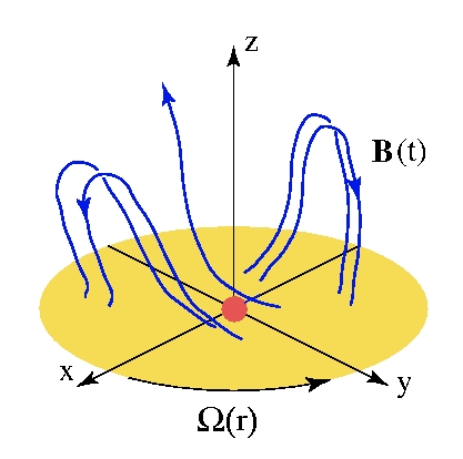
Figure 1: Sketch of an accretion disc threaded by open and closed magnetic field lines. Differential rotation of the disc will act to rapidly give an axisymmetric field configuration considered in this work.

2 Theory

2.1 Basic Equations

The plasma flows are assumed to be described by the equations of non-relativistic magnetohydrodynamics (MHD). In a non-rotating reference frame the equations are

$$\frac{\partial\rho}{\partial t}+\nabla\cdot\left(\rho\mathbf{v}\right)=0~{},$$ (1a)

$$\frac{\partial\rho\mathbf{v}}{\partial t}+\nabla\cdot\mathcal{T}=\rho\mathbf{g}~{},$$ (1b)

$$\frac{\partial\mathbf{B}}{\partial t}+c\>\nabla\times\mathbf{E}=0~{},$$ (1c)

$$\frac{\partial\left(\rho S\right)}{\partial t}+\nabla\cdot\left(\rho\mathbf{v}S\right)=\mathcal{Q}~{}.$$ (1d)

Here, $\rho$ is the mass density, $S$ is the specific entropy, $\mathbf{v}$ is the flow velocity, $\mathbf{B}$ is the magnetic field, $\mathcal{T}$ is the momentum flux density tensor, $\mathbf{E}$ is the electric field, $\mathcal{Q}$ is the rate of change of entropy per unit volume due to viscous and Ohmic heating in the disc, and $c$ is the speed of light. We assume that the heating is offset by radiative cooling so that $Q=0$. Also, $\mathbf{g}=-\left[GM/(r-r_{S})^{2}\right]\hat{r}$ (with $r_{S}\equiv 2GM/c^{2}$) is the gravitational acceleration due to the central mass $M$ with the Paczyński-Wiita (1980) correction relevant to neutron stars. We model the plasma as a non-relativistic ideal gas with equation of state

$$S=\ln\left(\frac{p}{\rho^{\gamma}}\right)~{},$$ (2)

where $p$ is the pressure and $\gamma=5/3$.

In most of this paper we use spherical $(r,\theta,\phi)$ coordinates. However, for some purposes cylindrical coordinates are advantageous, and they are denoted $(R,\phi,Z)$.

Both the viscosity and the magnetic diffusivity of the disc plasma are thought to be due to turbulent fluctuations of the velocity and magnetic field. Outside of the disc, the plasma is considered ideal with negligible viscosity and diffusivity. The turbulent coefficients are parameterized using the $\alpha$-model of Shakura and Sunyaev (1973). The turbulent kinematic viscosity is

$$\nu_{t}=\alpha_{\nu}\frac{c_{s}^{2}}{\Omega_{K}}~{},$$ (3)

where $c_{s}$ is the midplane sound speed, $\Omega_{K}$ is the Keplerian angular velocity at the given radii and $\alpha_{\nu}\leq 1$ is a dimensionless constant. Similarly, the turbulent magnetic diffusivity is

$$\eta_{t}=\alpha_{\eta}\frac{c_{s}^{2}}{\Omega_{K}}~{},$$ (4)

where $\alpha_{\eta}$ is another dimensionless constant. The ratio,

$$\mathcal{P}=\frac{\alpha_{\nu}}{\alpha_{\eta}}~{},$$ (5)

is the magnetic Prandtl number of the turbulence in the disc which is expected to be of order unity (Bisnovatyi-Kogan & Ruzmaikin 1976). Shearing box simulations of MRI driven MHD turbulence in discs indicate that ${\cal P}\sim 1$ (Guan & Gammie 2009).

The momentum flux density tensor is given by

$$\mathcal{T}_{ik}=p\delta_{ik}+\rho v_{i}v_{k}+\left(\frac{\mathbf{B}^{2}}{8\pi}\delta_{ik}-\frac{B_{i}B_{k}}{4\pi}\right)+\tau_{ik}~{},$$ (6)

where $\tau_{ik}$ is the viscous stress contribution from the turbulent fluctuations of the velocity and magnetic field. As mentioned we assume that these can be represented in the same way as the collisional viscosity by substitution of the turbulent viscosity. Moreover, we assume that the viscous stress is determined mainly by the gradient of the angular velocity because the azimuthal velocity is the dominant velocity of the disc. The leading order contribution to the momentum flux density from turbulence is therefore

$$\tau_{r\phi}=-\nu_{t}\rho r\sin\theta\frac{\partial\omega}{\partial r}~{},$$ (7a)

$$\tau_{\theta\phi}=-\nu_{t}\rho\sin\theta\frac{\partial\omega}{\partial\theta}~{},$$ (7b)

where $\omega=v_{\phi}/r\sin\theta$ is the plasma angular velocity.

The transition from the viscous-diffusive disc to the ideal plasma corona is handled by multiplying the viscosity and diffusivity by a dimensionless factor $\xi(\rho)$ which varies from $\xi=0$ for $\rho\leq 0.25\rho_{d}$ to $\xi=(4/3)(\rho/\rho_{d}-0.25)$ for $0.25\rho_{d}<\rho<\rho_{d}$ to $\xi=1$ for $\rho>\rho_{d}$ (see Appendix B of Lii, Romanova, & Lovelace 2012). The disc half-thickness $h$ is taken to be the vertical distance from $Z=0$ to the $0.5\rho_{d}$ surface.

2.2 Initial Conditions

2.2.1 Initial Magnetic Field

The initial magnetic field is described in cylindrical coordinates. This field is taken to be force-free in the sense that ${\bf J\times B}=0$ in the region $|Z|>0$ with ${\bf B}=(B_{R},B_{\phi},B_{Z})$, where $B_{R}=-R^{-1}\partial\Psi/\partial Z$ and $B_{Z}=R^{-1}\partial\Psi/\partial R$. Here, $\Psi(R,Z)$ is the flux function which labels the field lines, ${\bf B\cdot\nabla}\Psi=0$. This function satisfies the Grad-Shafranov equation,

$$\Delta^{*}\Psi(R,Z)=-H(\Psi){dH(\Psi)\over d\Psi}~{},$$ (8)

where

$$\Delta^{*}=\frac{\partial^{2}}{\partial R^{2}}-\frac{1}{R}\frac{\partial}{\partial R}+\frac{\partial^{2}}{\partial Z^{2}}~{},$$

and $H=H(\Psi)=RB_{\phi}(R,Z)$ is the poloidal current function (Lovelace et al. 1986). For simplicity we take the poloidal current to be proportional to the flux, $H(\Psi)=k\Psi,$ where $k$ is a constant (Newman et al. 1992). The relevant solution to equation (8) is

$$\Psi(R,Z)=A_{1}R\>J_{1}(a_{1}R)e^{-b_{1}|Z|}+A_{2}R\>J_{1}(a_{2}R)e^{-b_{2}|Z|}~{},$$ (9)

where $J_{1}$ is a Bessel function of the first kind, $A_{1}$, $A_{2}$ are integration constants and $a_{i}=(k^{2}+b_{i}^{2})^{1/2}$ for $i=1,2$. Qualitatively, the field appears as a number of loops threading the accretion disc. We have chosen the parameters $a_{i}$ such that three loops fit in our simulation region.

The solution (9) is valid in the region $|Z|>0$ and assumes that initially there is a thin current carrying disc in the $Z=0$ plane. The cusp in the initial field at $Z=0$ disappears rapidly in a time $t_{\rm init}\sim h^{2}/\eta_{t}=(\alpha_{\eta}\Omega_{K})^{-1}=P_{0}(2\pi\alpha_{\eta})^{-1}(r/r_{0})^{3/2}$ due to the diffusivity of the disc. Here, $r_{0}$ is the reference radius and $P_{0}$ the period of the Keplerian orbit at this radius as discussed in §2.4. We have assumed $h/R\approx c_{s}/v_{K}$ which neglects the magnetic compression of the disc discussed by Wang, Sulkanen, and Lovelace (1990). For most of the range of $r/r_{0}$ this time is much smaller than the field evolution time scale.

2.2.2 Matter Distribution

Initially the matter of the disc and corona are assumed to be in mechanical equilibrium (Romanova et al. 2002). The initial density distribution is taken to be barotropic with

$$\rho(p)=\begin{cases}p/T_{\rm{disc}}&p>p_{b}~{}~{}{\rm and}~{}~{}r\sin\theta\geq r_{b}~{},\\ p/T_{\rm{cor}}&p<p_{b}~{}~{}{\rm or}~{}~{}r\sin\theta\leq r_{b}~{},\end{cases}$$ (10)

where $p_{b}$ is the level surface of pressure that separates the cold matter of the disc from the hot matter of the corona and $r_{b}$ is the initial value of the inner radius of the disc. At this surface the density has an initial step discontinuity from value $p/T_{\rm{disc}}$ to $p/T_{\rm{cor}}$.

Because the density distribution is barotropic, the initial angular velocity is a constant on coaxial cylindrical surfaces about the $z-$axis. Consequently, the pressure can be determined from Bernoulli’s equation,

$$F(p)+\Phi+\Phi_{c}=\rm{const}~{},$$ (11)

where $\Phi=-GM/|r-r_{c}|$ is the gravitational potential with the Paczyński-Wiita correction, $\Phi_{c}=\int_{r\sin\theta}^{\infty}\xi d\xi~{}\omega^{2}(\xi)$ is the centrifugal potential, which depends only on cylindrical radius $R=r\sin\theta$, and

$$F(p)=\begin{cases}T_{\rm{disc}}\ln(p/p_{b})&p>p_{b}~{}~{}{\rm and}~{}~{}r\sin\theta\geq r_{b}~{},\\ T_{\rm{cor}}\ln(p/p_{b})&p<p_{b}~{}~{}{\rm or}~{}~{}r\sin\theta\leq r_{b}~{}.\end{cases}$$ (12)

2.2.3 Angular Velocity

Initially the inner edge of the disc is located at $r_{b}=5r_{0}$ in the equatorial plane, where $r_{0}$ is a reference length discussed below. The initial angular velocity of the disc is slightly sub-Keplerian,

$$\Omega\left|{}_{\theta=\pi/2}\right.=(1-0.003)\Omega_{K}(r)\hskip 28.45274ptr>r_{b}~{},$$ (13)

Inside of $r_{b}$, the matter rotates rigidly with angular velocity

$$\Omega\left|{}_{\theta=\pi/2}\right.=(1-0.003)\Omega_{K}(r_{b})\hskip 28.45274ptr\leq r_{b}.$$ (14)

The corotation radius $r_{\rm cr}$ is the radius where the angular velocity of the disc equals that of the star; that is, $r_{\rm cr}=(GM_{*}/\Omega_{*}^{2})^{1/3}$. In this study we have chosen this radius to be the initial inner radius of the disc with $r_{\rm cr}=5r_{0}$.

2.3 Boundary Conditions

Our simulation region has four boundaries: The surface of the star, the midplane of the disc, the rotation axis, and the external boundary. For each dynamical variable we impose boundary conditions consistent with our physical assumptions.

We assume axisymmetry as well as symmetry about the equatorial plane. On the star and the external boundary we want to allow fluxes and so impose free boundary conditions $\partial{\cal F}/\partial r=0$, where $\cal F$ are the dynamical variables. In addition, along the external boundary in the disc region $\theta=72^{\circ}-90^{\circ}$, we allow matter to inflow but the inflowing matter has zero magnetic flux. In the coronal region $\theta=0^{\circ}-72^{\circ}$ we allow matter, entropy and magnetic flux to exit the simulation region.

In addition to the boundary conditions, which are required for the well-posedness of our problem, we impose additional conditions on variables to eliminate numerical artifacts in the simulations. For instance, we require that the radial velocity at the surface of the star be negative. Thus there there is no outflow of matter, angular momentum, or energy from the star. We also require that along the external boundary the radial velocity be inwards inside the disc and outwards outside the disc so the disc matter will tend to accrete and matter in the corona will tend to be ejected.

Figure 2 shows the grid used in the described simulations. There are $N_{\theta}=30$ constant width cells in the $\theta-$direction. In the $r-$direction, the $N_{r}=67$ grid cells increase in width as $dr_{j+1}=(1+0.0523)dr_{j}$ so as to give curvlinear rectangles with approximately equal sides (Ustyugova et al. 2006). The dependence of our results on the grid resolution is discussed in Appendix A.

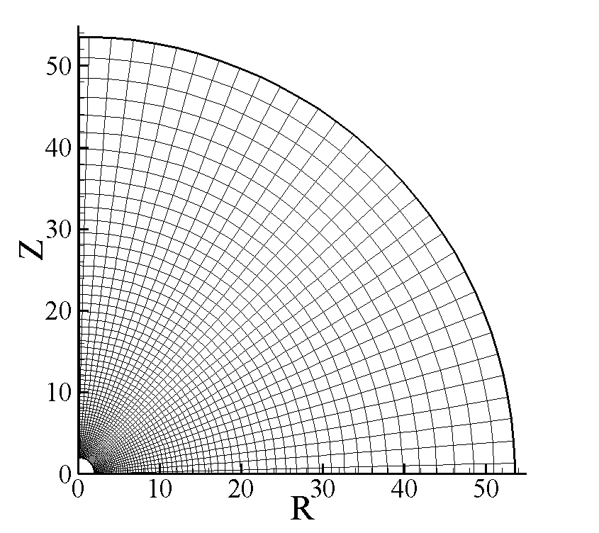
Figure 2: Grid used in the simulations.

2.4 Dimensional Variables

Parameters	Symbol	Value
mass	$M_{*}$	$2.8\times 10^{33}$ g
length	$r_{0}$	$1.0\times 10^{6}$cm
magnetic field	$B_{0}$	$10^{8}$ G
time	$P_{0}$	$4.6\times 10^{-4}$s
velocity	$v_{0}$	$1.4\times 10^{10}$cm/s
density	$\rho_{0}$	$1.3\times 10^{-5}$ g/cm3
accretion rate	$\dot{M}_{*}$	$2.8\times 10^{-9}$ $M_{\odot}$/yr
disc power	$\dot{E}_{0}$	$1.66\times 10^{37}$ erg/s

Table 1: Mass, length, and magnetic field scales of interest and the corresponding scales of other derived quantities

The MHD equations are written in dimensionless form so that the simulation results can be applied to different types of stars. The mass of the central star is taken as the reference unit of mass, $M_{0}=M_{*}$. The reference length, $r_{0}$, is taken to be half the radius of the star. The initial inner radius of the disc is $r_{b}=5r_{0}$. The reference value for the velocity is the Keplerian velocity at the radius $r_{0}$, $v_{0}=(GM_{0}/r_{0})^{1/2}$. The dimensionless temperature is $T/v_{0}^{2}$. The reference time-scale is the period of rotation at $r_{0}$, $P_{0}=2\pi r_{0}/v_{0}$. From the MHD equations, we get the relation $\rho_{0}v_{0}^{2}=B_{0}^{2}$, where $B_{0}$ is a reference magnetic field and $\rho_{0}$ is a reference density both at $r_{0}$. We take the reference magnetic field $B_{0}$ to be such that the reference density is appropriate for the considered star. The reference mass accretion rate is $\dot{M}_{0}=\rho_{0}v_{0}r_{0}^{2}$. The reference disc accretion power is $\dot{E}_{0}=GM_{0}\dot{M}_{0}/r_{0}$. The initial dimensionless temperature in the disc is $T_{\rm{disc}}=(p/\rho)_{\rm{disc}}=5\times 10^{-4}$, and the initial temperature in the corona is $T_{\rm{cor}}=(p/\rho)_{\rm{cor}}=0.5$.

Results obtained in dimensionless form can be applied to objects with widely different sizes and masses. However, the present work focuses on neutron stars with the typical values shown in Table 1.

3 Results

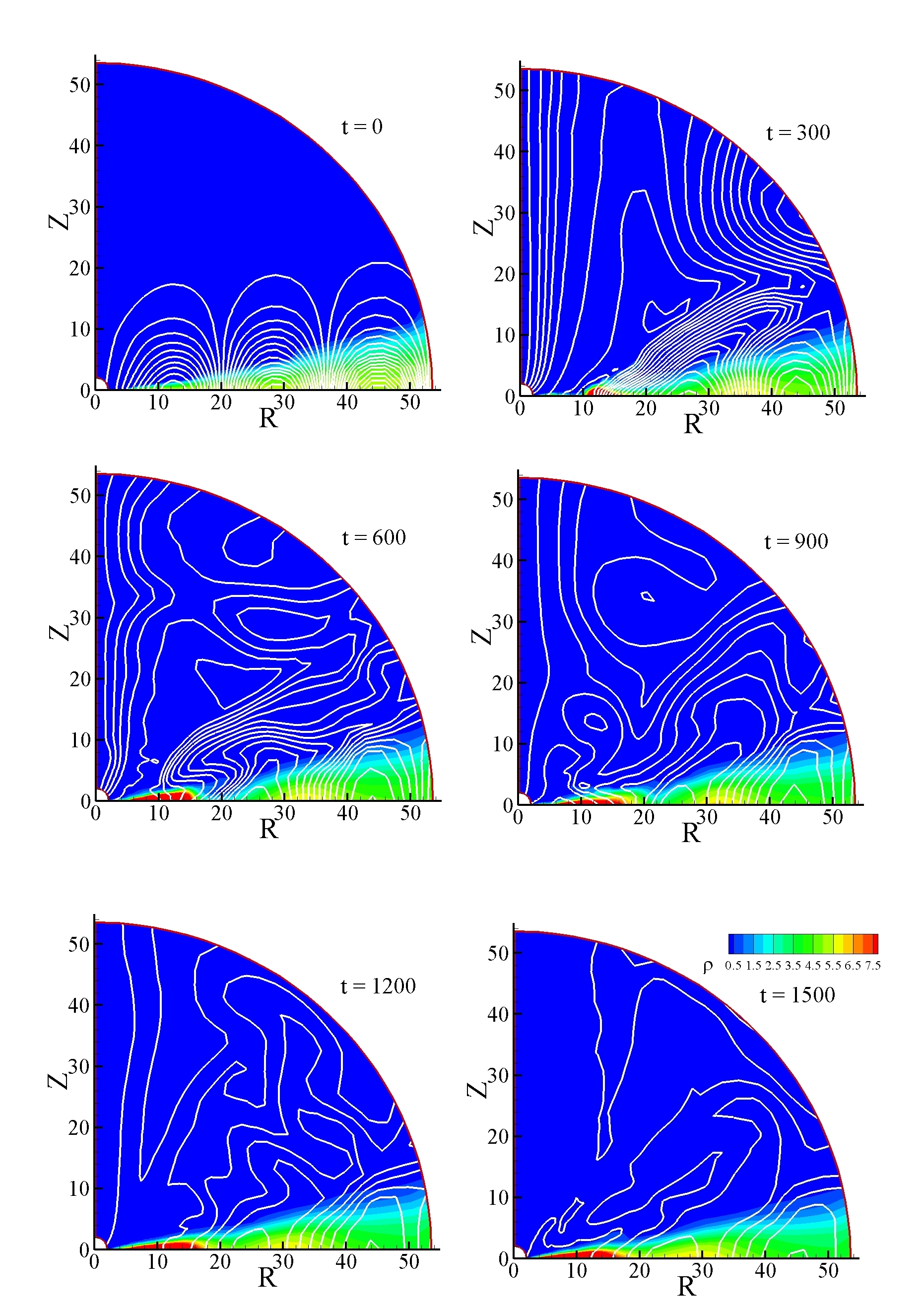
Figure 3: Plot of poloidal magnetic field lines (white) and matter density (colour) for $\alpha_{\nu}$ = 0.1 and $\alpha_{\eta}$ = 0.1 at $t=0,~{}=300,~{}..,1500$, where $t$ is the time measured in units of $P_{0}$ which is the period of the Keplerian orbit at the reference radius $r_{0}$ (see §2.4). By $t=300$ sufficient matter has fallen into the star to drag in the magnetic field. The latter forms a well collimated jet along the axis and a wind along the disc. This persists for some time, but eventually decays due to magnetic field reconnection and annihilation.

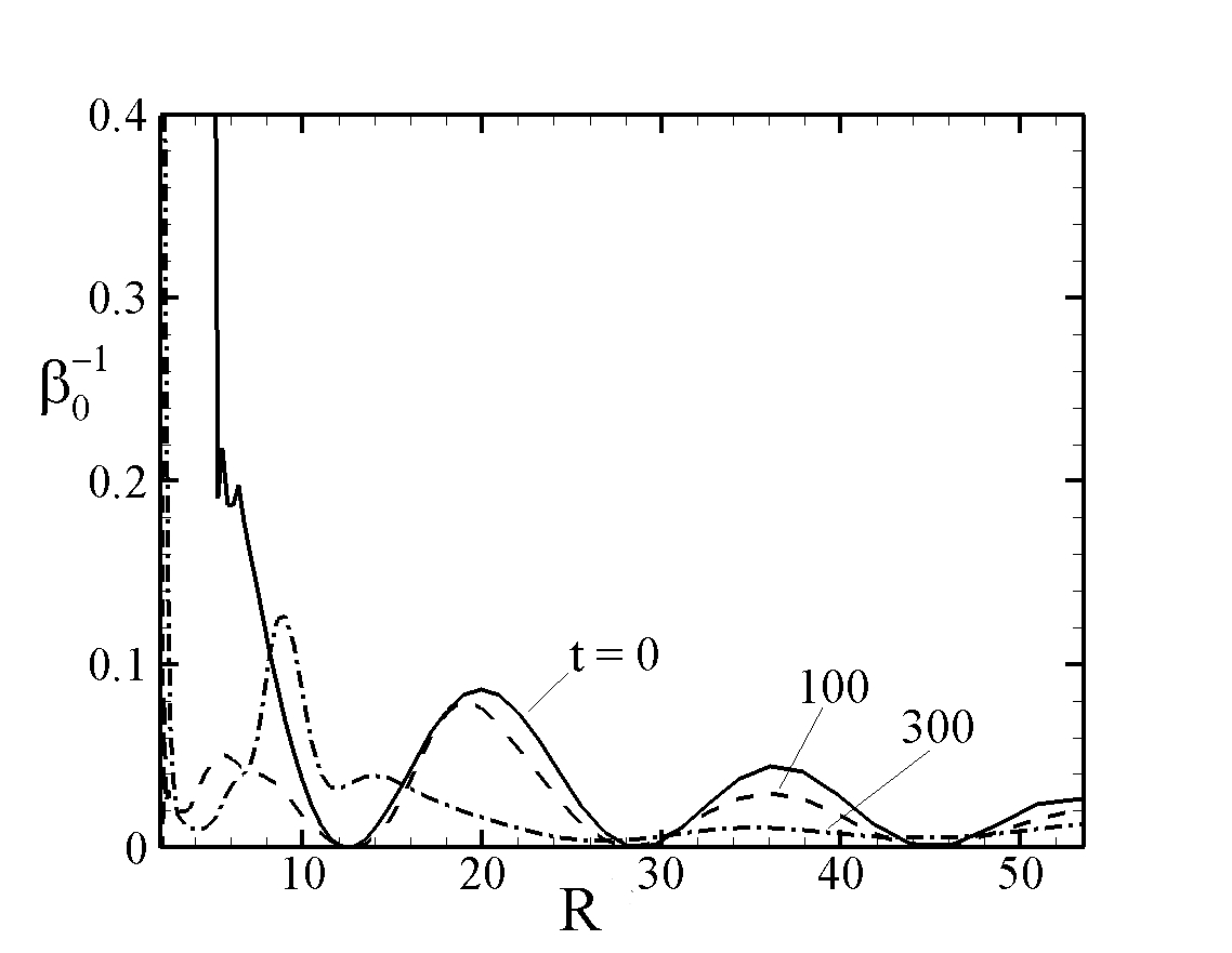
Figure 4: The ratio of magnetic pressure to the plasma pressure $\beta_{0}^{-1}$ in the disc midplane at $t=0$ (full), $t=100$ (dashed) and $t=300$ (dot-dashed) for $\alpha_{\nu}=0.1$ and $\alpha_{\eta}=0.1$.

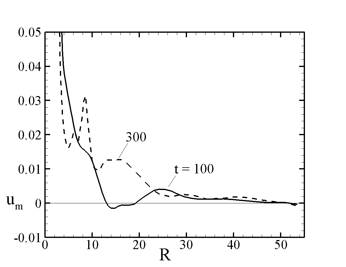
Figure 5: Radial accretion speed of the disc matter (equation 16) at $t=100$ (full) and $t=300$ (dashed) for $\alpha_{\nu}=0.1$ and $\alpha_{\eta}=0.1$.

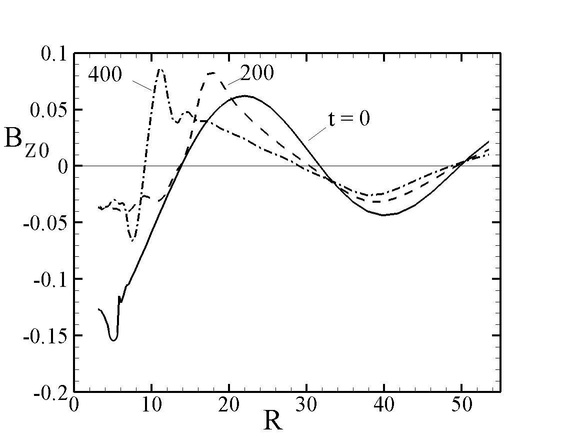
Figure 6: The magnetic field $B_{Z}(R,Z=0)$ along the disc midplane at $t=0$ (full), $t=200$ (dashed) and $t=400$ (dot-dashed) for $\alpha_{\nu}=0.1$ and $\alpha_{\eta}=0.1$.

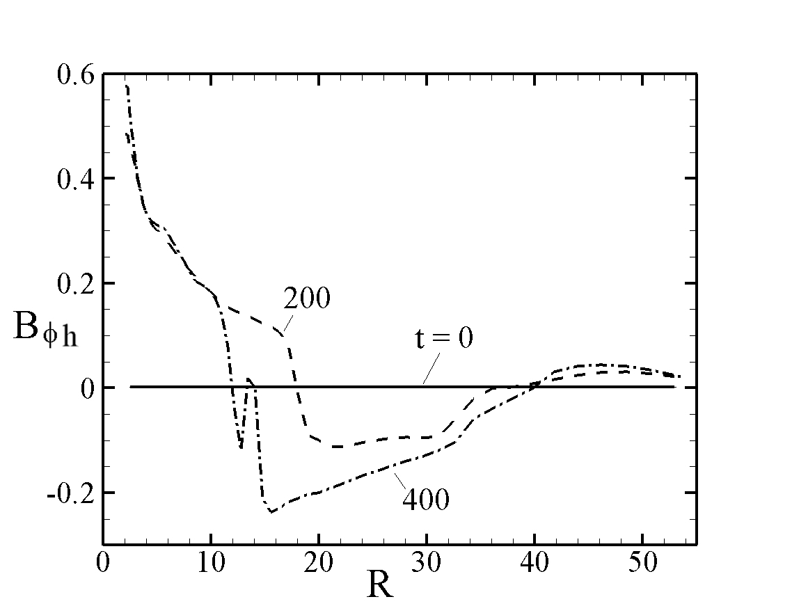
Figure 7: The toroidal magnetic field $B_{\phi}(R,Z=h)$ at the disc surface at $t=0$ (full), $t=200$ (dashed) and $t=400$ (dot-dashed) for $\alpha_{\nu}=0.1$ and $\alpha_{\eta}=0.1$.

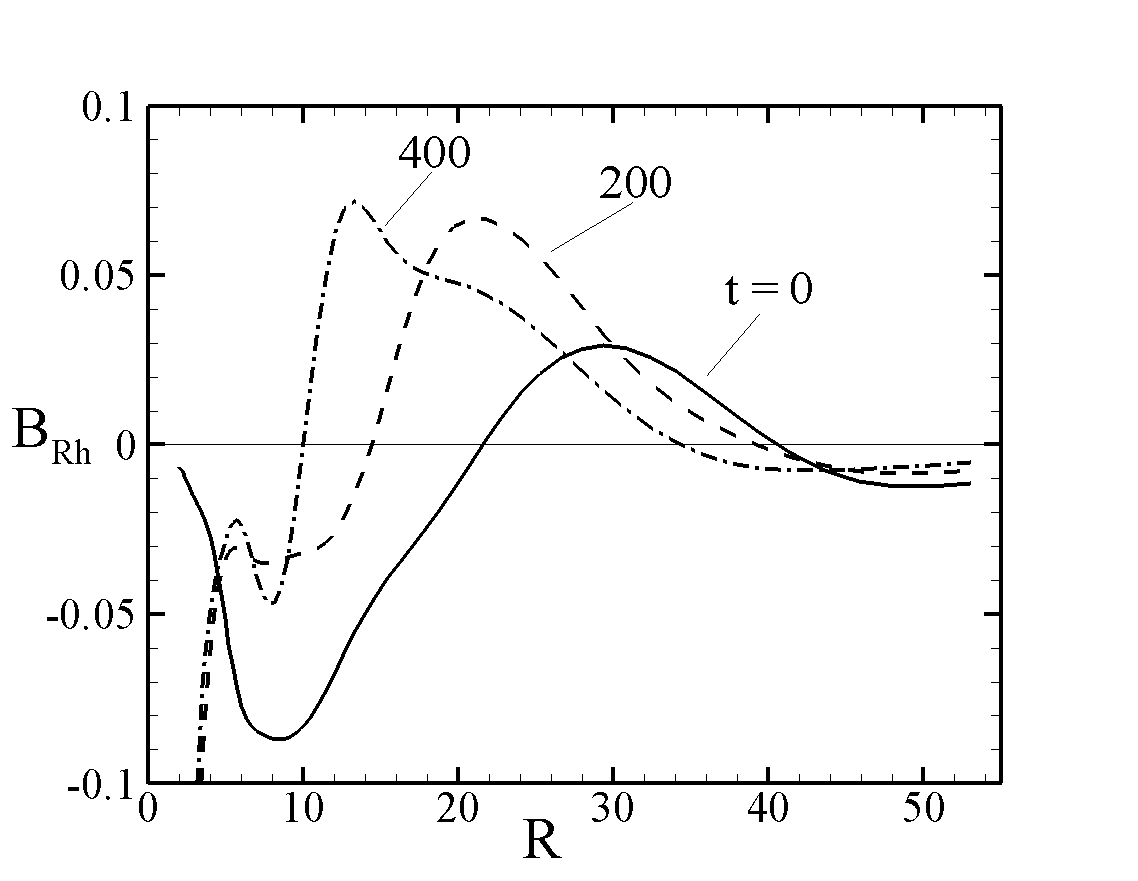
Figure 8: The radial component of the magnetic field $B_{R}(R,Z=h)$ at the disc surface at $t=0$ (full), $t=200$ (dashed) and $t=400$ (dot-dashed) for $\alpha_{\nu}=0.1$ and $\alpha_{\eta}=0.1$. This quantity has an important role in determining the diffusive advection of the magnetic field $u_{B\eta}$ (equation 26).

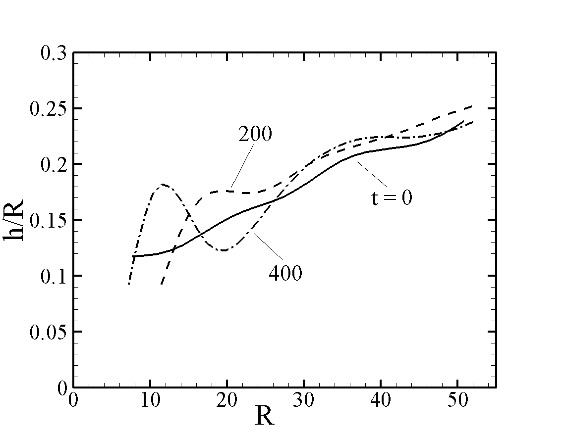
Figure 9: The radio of the disc half thickness to the radius $h/R$ as a function of $R$.

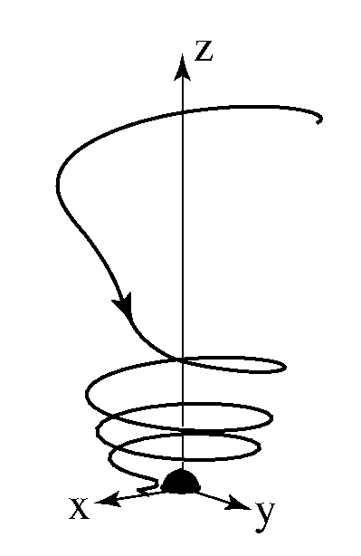
Figure 10: Three dimensional view of a magnetic field line originating from the disc at $R=6$ at time $t=300$. The twist of the field line is such that the field transports angular momentum out of the disc. That is, $B_{Z}B_{\phi}<0$.

We have carried out a large number of simulation runs for different values of the viscosity $0.05\leq\alpha_{\nu}\leq 0.3$ and diffusivity $0.01\leq\alpha_{\eta}\leq 0.3$ parameters and find that the simulations exhibit similar qualitative behaviour. Figure 3 shows the evolution of the poloidal field projections for a representative case where $\alpha_{\nu}=0.1$ and $\alpha_{\eta}=0.1$. The field lines of the innermost loop are pulled in towards the star by the accreting disc matter. When this loop reaches the star’s surface it opens up. The inner half of the loop extends vertically upwards from the star, supporting a magnetically dominated jet along the $z-$axis. The outer half of the loop threading the disc projects outwards from the disc at about $45^{\circ}$ to the disc normal, and it supports a magnetic disc wind. The middle and outer magnetic loops move inward only gradually, and they decrease in strength due to field line annihilation inside the disc.

Figure 4 shows the radial dependence of the inverse “plasma beta” which is the ratio of the magnetic pressure to the plasma pressure at the disc midplane,

$$\beta_{0}^{-1}={B_{Z0}^{2}\over 8\pi p(R,0)}~{},$$ (15)

where $B_{Z0}\equiv B_{Z}(R,Z=0)$. Note that $\beta_{0}^{-1}=(v_{A0}/c_{s0})^{2}/2$, where $v_{A0}=B_{Z0}/\sqrt{4\pi\rho}$ is the midplane Alfvén speed and $c_{s0}$ is the midplane sound speed. For the assumed symmetry about the equatorial plane $B_{Z}$ is the only non-vanishing field component at $Z=0$. Initially $\beta_{0}^{-1}$ is significantly less than unity over most of the disc ($R\gtrsim 5$). Consequently, the magneto-rotational instability would be expected to occur in an actual disc with the same parameters (Balbus & Hawley 1998). At later times, $[B_{Z}(R,0)]^{2}$ increases but the plasma pressure also increases so that the change in $\beta_{0}^{-1}$ are not very large.

3.1 Opening of Field Loops and Field Annihilation

The initial three poloidal field loops ($t=0$ panel of Figure 3), have footpoints at the approximate radii $R_{k}=5,~{}20,~{}35,~{}\&~{}50$ ($k=1,..,4$). The time-dependent opening of large-scale magnetic field loops with footpoints at different radii in a Keplerian disc has been well analyzed (Newman, Newman, & Lovelace 1992; Lynden-Bell & Boily 1994; Romanova et al. 1998; Ustyugova et al. 2000; Lovelace et al. 2002). We use the numerical condition of Lynden-Bell and Boily (1994) that a field loop opens after there is a differential rotation of the footpoints by $>3.63$ radians. For each loop, the differential rotation in a time $t_{k}$ is $\Delta\phi=t_{k}[\Omega_{K}(R_{k})-\Omega_{K}(R_{k+1})]$. With $\Delta\phi=3.63$ we obtain the opening times for the three loops, $t_{1}=40.8$, $t_{2}=329$, and $t_{3}=760$ in our dimensionless units. The observed rapid opening of the first loop (Figure 3) agrees qualitatively with $t_{1}$. The fact the second loop does not open in a time $\sim t_{2}$ may be explained by the overlying magnetic field of the first loop. The long time $t_{3}$ required for the opening of the third loop means the diffusion of the magnetic field has sufficient time to cause significant field annihilation.

The time scale for the field to diffuse over a distance $\Delta R_{k}/2=(R_{k+1}-R_{k})/2$ can be estimated as $\tau_{k}\approx(\Delta R_{k})^{2}/(4\eta_{t})$, where $\eta_{t}$ is evaluated at $\overline{R}_{k}=(R_{k}+R_{k+1})/2$. For $\alpha_{\eta}=0.1$, we find $\tau_{1}\approx 2500$, $\tau_{2}\approx 1700$, and $\tau_{3}\approx 1400$. Note that $\tau_{3}$ for the outer loop is less than the duration of our runs so that the magnetic field decays significantly before the end of the runs.

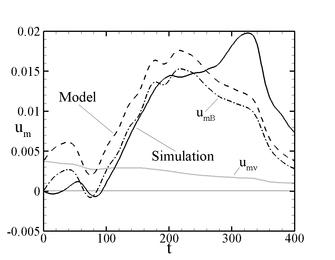
Figure 11: The solid curve shows the average accretion speed of the disc matter at the maximum of $B_{Z}(R,Z=0)$ from the simulations for $\alpha_{\nu}=0.1=\alpha_{\eta}$. The initial radius of the maximum is $R=22$. The dashed curve is from the advection model (eqns. 19 and 20)) with parameters $C_{1}=0.05$ and $C_{2}=0.2$. The model breaks down when the maximum approaches the star and interacts strongly with it. This happens at different times for different viscosity and diffusivity values.

3.2 Matter Advection in the Disc

Figure 5 shows the average accretion speed $u_{m}$ of the disc matter as a function of $R$ at different times, where

$$u_{m}\equiv-{1\over\sigma(R)}\int_{-h}^{h}dZ\rho(R,Z)v_{R}(R,Z)~{}.$$ (16)

Here,

$$\sigma(R)=\int_{-h}^{h}dZ\rho(R,Z)~{},$$ (17)

is the surface mass density of the disc. The conservation of mass gives

$${\partial(R\sigma)\over\partial t}-{\partial(R\sigma u_{m})\over\partial R}=-{1\over\pi}{\delta\dot{M}_{w}\over\delta R}~{},$$ (18)

where $\delta\dot{M}_{w}/\delta R=2\pi R(\rho v_{z})_{Z=h}$ is the mass outflow rate from the top surface of the disc to the wind. The mass accretion rate to the star from the upper half-space is $\dot{M}_{*}=(\pi R\sigma u_{m})_{R=r_{0}}$. We find that the ratio of the time-averaged mass loss rate of the wind is typically small compared to $\dot{M}_{*}$.

Figure 6 shows the midplane magnetic field $B_{Z}(R,0)$ at different times. Because of the assumed symmetry of the magnetic field about the equatorial plane, this is the only non-zero field component at $Z=0$.

Matter advection in the disc is measured by $u_{m}(R,t)$, which is determined by the disc’s turbulent viscosity (which causes the radial outflow of angular momentum) and by the torque of the large-scale magnetic field (which causes a vertical outflow of angular momentum to magnetic jets or winds). This is described by a simple analytic model where

$${u}_{\rm{m}}=u_{m\nu}+u_{mB}~{},$$ (19)

where

$$u_{m\nu}=3C_{1}\alpha_{\nu}\left(\frac{h}{R}\right)^{2}v_{K},~{}~{}u_{mB}={-C_{2}B_{\phi h}B_{Z0}\over\pi v_{K}\sigma}~{},$$ (20)

(Lovelace et al. 2009; 1994), where $h$ is the half-thickness of the disc, $v_{K}=(GM/R)^{1/2}$ is the Keplerian velocity, $\sigma$ is the surface mass density of the disc, $B_{\phi h}=B_{\phi}(R,h)$ is the toroidal magnetic field at the disc surface, $B_{Z0}=B_{Z}(R,Z=0)$ is the midplane magnetic field, and $C_{1}$ and $C_{2}$ are dimensionless constants of the order of unity. The first term represents the accretion speed contribution due to the turbulent viscosity of the disc, while the second term the accretion speed contribution due to the outflow of angular momentum from the disc surfaces due to the twisted magnetic field in the corona.

Figure 7 shows the profiles of the toroidal magnetic field at the disc surface $B_{\phi}(R,h)$ at a sequence of times. This quantity is important for the outflow of angular momentum from the disc which in turn determines the magnetic contribution to the accretion speed $u_{mB}$ in equation (20).

Figure 8 shows the radial profiles of $B_{Rh}$ at a sequence of times. This quantity is important for the radial diffusion of the magnetic field as discussed below in §3.3 Figure 9 shows the radial variation of $h/R$ at a sequence of times.

Figure 10 shows that the twist of a sample magnetic field line above the disc is such that $B_{\phi h}B_{Z0}<0$ which corresponds the to outflow of angular momentum from the disc.

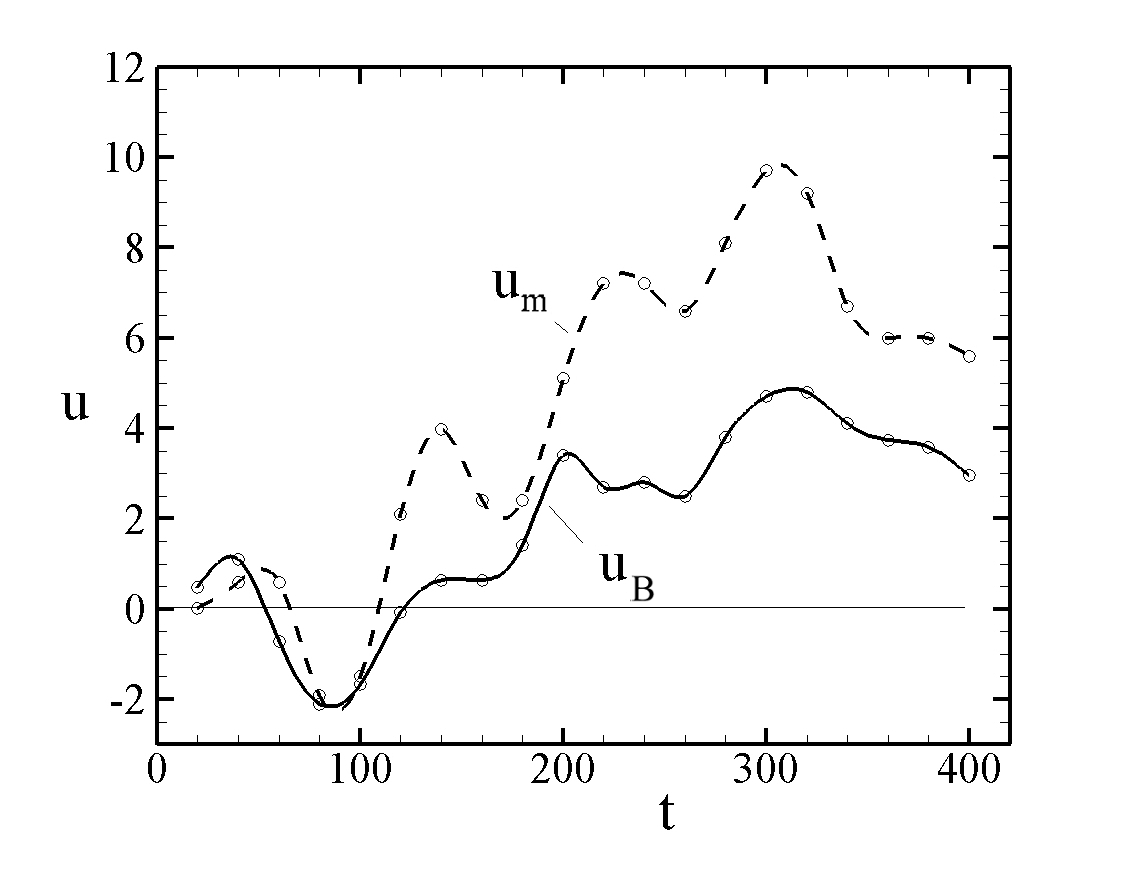
Figure 12: Accretion speed of the magnetic field $u_{B}$ in the equatorial plane derived from the motion of the innermost zero crossing of $B_{Z}(R,Z=0,t)$ and the matter accretion speed $u_{\rm m}$ at the same location for $\alpha_{\nu}=0.1=\alpha_{\eta}$. The initial radius of zero crossing is $R_{\rm O}(t=0)=13.7$.

We find that during early times ($t\lesssim 400$), the $B_{Z}(R,0)$ field “propagates” inwards towards the star as shown in Figure 6. We study this motion by measuring the positions of the inner maximum of $B_{Z}(R,0)$ as a function of time. The maximum moves inwards until interactions with the star cause a more complicated behavior. At the $B_{Z}(R,0)$ maximum at a given time $t$, we calculate the accretion speed $u_{\rm m}(R,t)$ in our simulation data using equation (16). We also calculate $B_{\phi h}(R,t)$, $B_{Z0}(R,t)$, $h/R$, and $\sigma(R,t)$ which permits us to compare the observed accretion speed with the prediction of the advection model (equations 19 and 20). We find that the reasonable values of $C_{1}=0.4$ and $C_{2}=0.2$ give satisfactory agreement between the model and our various simulation runs for $t\lesssim 400$.

Figure 11 shows the model and the measured simulation accretion speeds for sample cases.

3.3 Magnetic Field Advection in the Disc

The advection of the poloidal magnetic field is described by the equation

$${\partial(R\overline{B}_{Z})\over\partial t}-{\partial(R\overline{B}_{Z}u_{Bi})\over\partial R}={\partial\over\partial R}\left(-{\eta_{t}RB_{Rh}\over h}+\eta_{t}R{\partial\overline{B}_{Z}\over\partial R}\right)~{},$$ (21)

(Lovelace et al. 1994), where $B_{Rh}=B_{R}(R,Z=h)$. For simplicity we have neglected terms of order $|\partial h/\partial R|$ relative to unity. Here,

$$u_{Bi}\equiv-\int_{-h}^{h}dZB_{Z}(R,Z)v_{R}(R,Z)\bigg{/}\int_{-h}^{h}dZB_{Z}(R,Z),$$ (22)

is the magnetic field advection speed of an ideal, perfectly conducting disc ($\eta_{t}=0$). Note that the matter advection speed $u_{m}$ is a density weighted average over the disc thickness of $-v_{R}$ whereas $u_{Bi}$ is an average of $-v_{R}$ weighted by $B_{Z}$. For smooth profiles of $\rho$ and $B_{Z}$ the two speeds will be be comparable.

The vertical magnetic flux threading the disc inside the first O-point where $\overline{B}_{Z}(R_{\rm O},0)=0$ (or between successive O-points) decreases in general with time due to the diffusivity. From equation (21) we have

$${d\over dt}\int_{0}^{R_{\rm O}}RdR\overline{B}_{Z}=\left(-{\eta_{t}RB_{Rh}\over h}+\eta_{t}R{\partial\overline{B}_{Z}\over\partial R}\right)_{R=R_{\rm O}}~{}.$$ (23)

For example, for $\overline{B}_{Z}<0$ inside $R_{\rm O}$, both terms on the right-hand side of equation (23) are seen to be positive so that the magnitude of the flux decreases.

For $\eta_{t}>0$ the field advection speed is the sum of the ideal and diffusive contributions,

$$u_{B}=u_{Bi}+u_{B\eta}~{},$$ (24)

with

$${\partial(R\overline{B}_{Z})\over\partial t}-{\partial(R\overline{B}_{Z}u_{B})\over\partial R}=0~{}.$$ (25)

Here

$$u_{B\eta}=-{\eta_{t}B_{Rh}\over h\overline{B}_{Z}}+{\eta_{t}\over\overline{B}_{Z}}{\partial\overline{B}_{Z}\over\partial R}$$ (26)

is the diffusive advection speed.

From our simulation data we can calculate the advection speed of the magnetic field $u_{Bi}$ by tracking the location $R_{\rm O}(t)$ of the $B_{Z}(R,Z=0)$ zero crossings which occur at “O-points” of the poloidal magnetic field ${\bf B}_{p}$. Close to the zero crossing, $B_{Z}(R,0)={\rm const}(R-R_{\rm O})$ is an odd function of $R-R_{\rm O}$. Furthermore, $\overline{B}_{Z}$ is also an odd function of $R-R_{O}$. Thus $u_{B\eta}$ is an odd function about the O-point proportional to $(R-R_{\rm O})^{-1}$ because of the $\overline{B}_{Z}$ denominators in equation (26). The magnetic field moves symmetrically inward towards the O-point where it annihilates. The mathematical singularity is smoothed out by the finite grid. The magnetic field inside a current-carrying resistive wire behaves in the same way. Consequently, at $R=R_{\rm O}$ we have $u_{B\eta}=0$. The diffusivity has no influence on the motion of the O-point. That is, $dR_{\rm O}/dt=-u_{B}=-u_{Bi}$.

We can compare field advection speed $u_{B}$ (at an O-point) to the matter advection speed $u_{\rm m}$ at the same location. As mentioned these two speeds are expected to be comparable.

Figure 12 shows sample comparisons of $u_{B}$ and $u_{\rm m}$. For a smaller diffusivity with fixed viscosity the difference between matter and field accretion speeds is smaller. For a larger viscosity relative to diffusivity, $u_{m}$ is significanty larger than $u_{B}$.

3.4 Late times

At late times ($t\gtrsim 1000$), the magnetic field decays appreciably owing to reconnection and field annihilation. Consequently the accretion speed is due mainly to the disc viscosity,

$${u}_{\rm m}\approx u_{m\nu}~{}.$$ (27)

The mass accretion rate to the star from the top half space is $\dot{M}_{*}=\pi(R\Sigma u_{\rm m})_{*}$, where $\Sigma$ is the surface mass density of the disc and the asterisk subscript indicates evaluation outside the star.

Figure 13 shows the time dependence of the accretion rate to the star and the mass outflow rate in the wind for two viscosity values and $\alpha_{\eta}=0.1$. For $0.05\leq\alpha_{\nu}\leq 0.3$ we find that $\dot{M}_{*}$ at late times ($t>1000$) is approximately proportional to $\alpha_{\nu}$. At late times $\dot{M}_{*}$ is independent of the diffusivity $\alpha_{\eta}$.

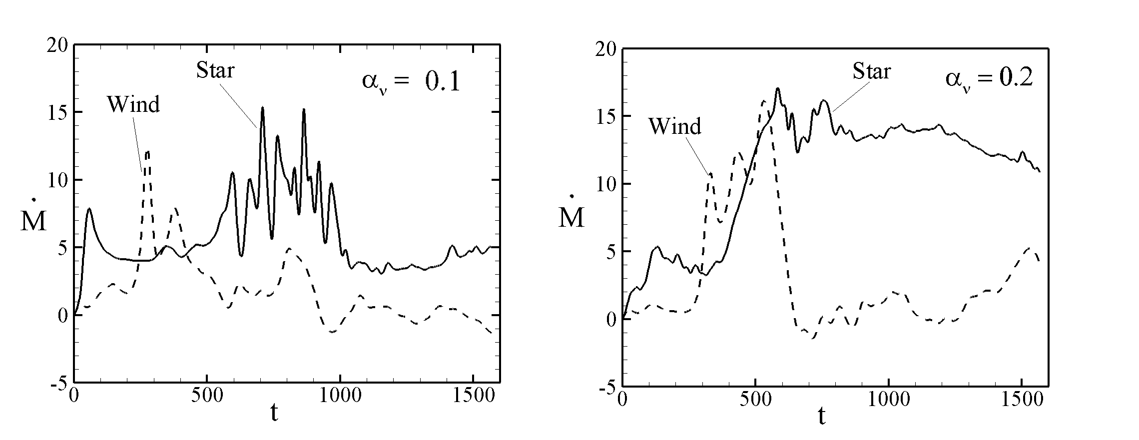
Figure 13: Dimensionless mass accretion rate to the star $\dot{M}_{*}$ and mass loss rate to the wind $\dot{M}_{w}$ for two viscosities with same diffusivity $\alpha_{\eta}=0.1$.

3.5 Jet and Wind

In this work we observe both a collimated jet along the $Z-$axis and an uncollimated disc wind.

3.5.1 Jet

The fluxes of angular momentum and energy through the spherical surface $[r=44,~{}0^{\circ}\leq\theta\leq 21^{\circ}]$ are shown in Figure 14 The angular momentum flux can be separated into a part from the matter and a part due to the magnetic field,

$$\dot{L}=\dot{L}_{m}+\dot{L}_{f}=\int d{\bf S}\ \cdot\left(\rho r\sin(\theta)v_{\phi}\mathbf{v}_{p}-\frac{r\sin(\theta)B_{\phi}\mathbf{B}_{p}}{4\pi}\right).$$ (28)

Similarly, the energy flux can be separated into contributions carried by the matter and that carried by the Poynting flux,

$$\dot{E}=\dot{E}_{m}+\dot{E}_{f}=\int d{\bf S}\ \cdot\left(\frac{1}{2}\rho{\bf v}^{2}\mathbf{v}_{p}+\frac{c}{4\pi}\mathbf{E}\times\mathbf{B}\right).$$ (29)

The jet is strongly dominated by the electromagnetic field: The angular momentum flux is carried predominantly by the magnetic field and the energy flux is carried predominantly by the Poynting flux. Such jets were hypothesized by Lovelace (1976) and first observed in axisymmetric MHD simulations by Ustyugova et al. (2000).

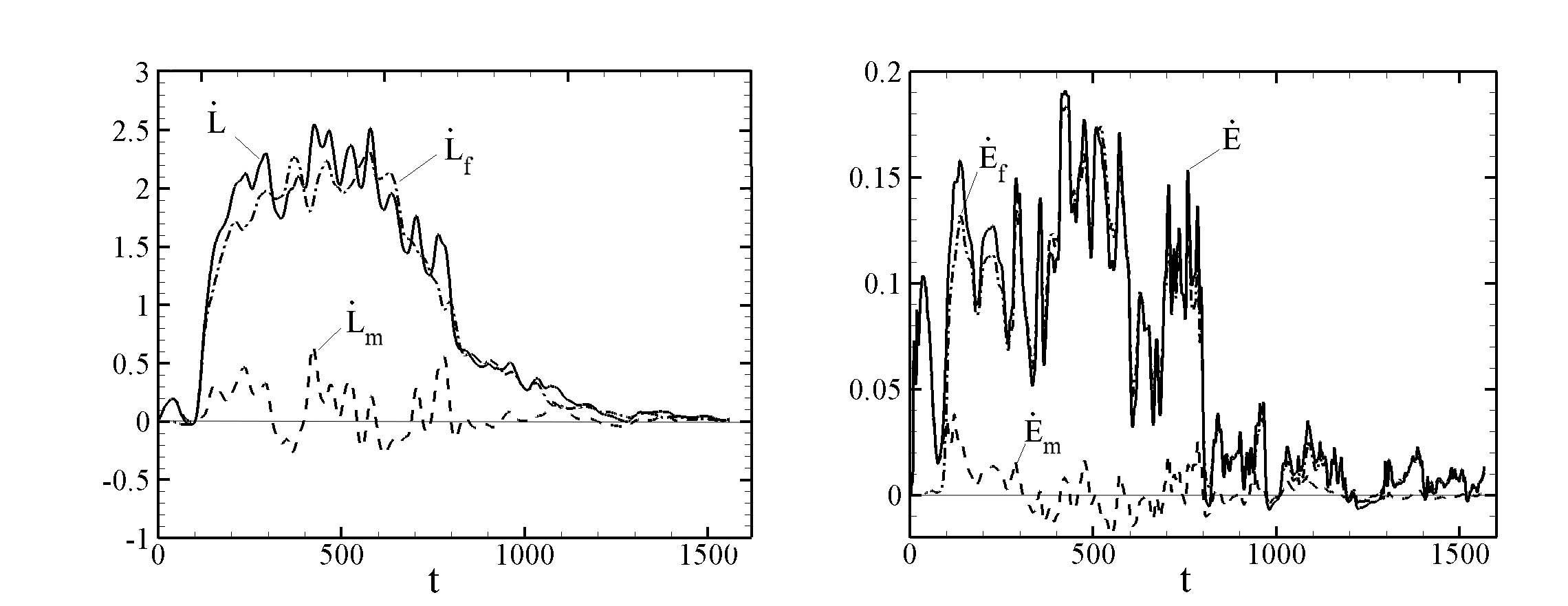
Figure 14: - Left panel: The jet angular momentum flux carried by the matter (dashed curve), the magnetic field (dot-dashed curve), and the total flux (solid curve) for $\alpha_{\nu}=0.1$ and $\alpha_{\eta}=0.1$. Right-panel: The jet energy flux carried by the matter (dashed curve), the Poynting flux (dot-dashed curve), and the total flux (solid curve) for $\alpha_{\nu}=0.1$ and $\alpha_{\eta}=0.1$. The jet is strongly dominated by the Poynting flux.

3.5.2 Disc Wind

The rates of energy, angular momentum and mass flux through the surface $[r=44,~{}21^{\circ}\leq\theta\leq 72^{\circ}]$ is shown in Figure 15. We have chosen the upper bound for $\theta$ by requiring that the wind stay outside the disc.

Figure 14 shows the different components of the wind angular momentum flux and the components of the energy flux. The angular momentum and energy fluxes are dominated by the matter components. This is the opposite of the case for the jet.

Figure 14 shows the jet and wind total energy fluxes normalized to the “accretion power” $\dot{E}_{\rm acc}=GM_{*}\dot{M}_{*}/(2r_{*})$. The large initial values of the ratios results from the fact that $\dot{M}_{*}$ is initially zero. Note that the two ratios are comparable.

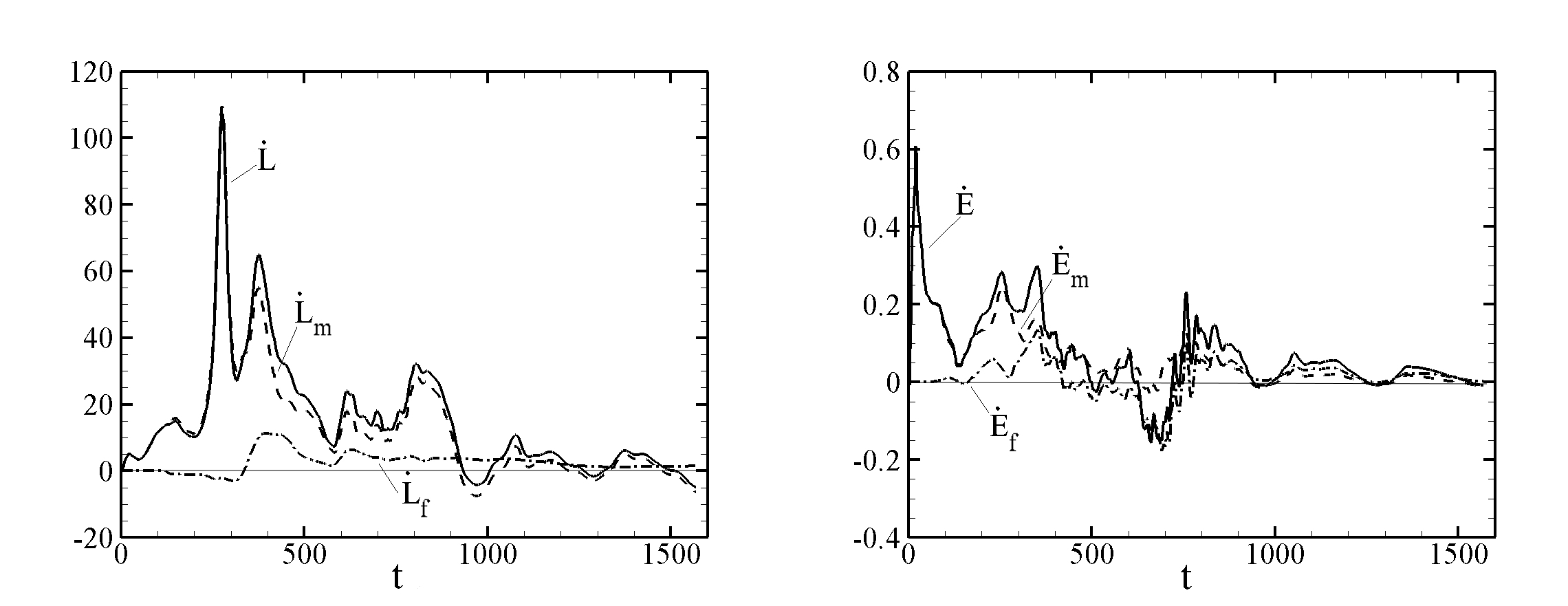
Figure 15: - Left panel: The wind angular momentum flux carried by the matter (dashed curve), the magnetic field (dot-dashed curve), and the total (solid curve) for $\alpha_{\nu}=0.1$ and $\alpha_{\eta}=0.1$. Right panel: The wind energy flux carried by the matter (dashed curve), the Poynting flux (dot-dashed curve), and the total flux(solid curve) for $\alpha_{\nu}=0.1$ and $\alpha_{\eta}=0.1$. The wind is strongly matter dominated.

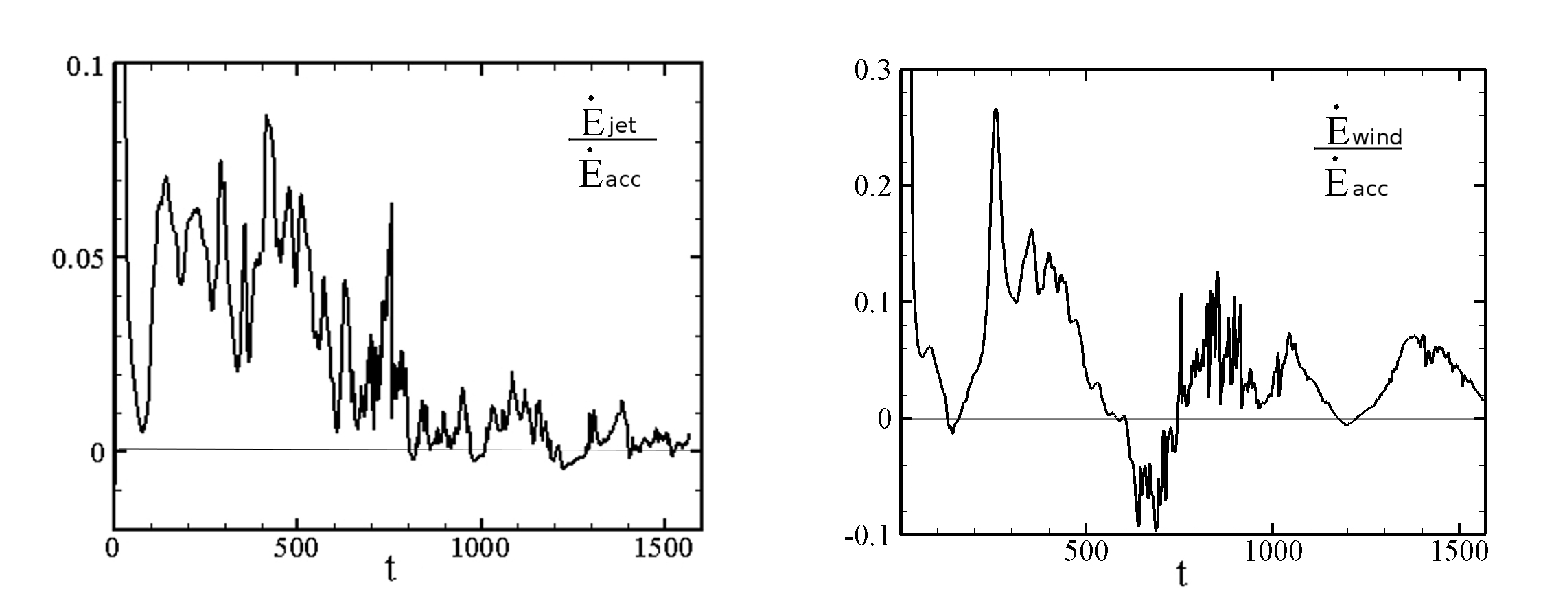
Figure 16: - Left panel: The total jet energy flux normalized by the “accretion power” $\dot{E}_{\rm acc}=GM_{*}\dot{M}_{*}/(2r_{*})$ for $\alpha_{\nu}=0.1$ and $\alpha_{\eta}=0.1$. Right panel: The total wind power also normalized by the accretion power $\dot{E}_{\rm acc}$ for $\alpha_{\nu}=0.1$ and $\alpha_{\eta}=0.1$. The large initial values of the ratios is due to the fact that the $\dot{M}_{*}$ is initially zero. The fact that $\dot{E}_{\rm wind}$ is temporarily negative is due to the fixed partition of the range of $\theta$ into wind and disc regions.

4 Conclusions

We have analyzed a set of axisymmetric MHD simulations of the evolution of a turbulent/diffusive accretion disc initially threaded by a weak magnetic field with midplane plasma beta $\beta_{0}$ is significantly larger than unity. The viscosity and magnetic diffusivity are modeled by two $\alpha$ parameters, one for the viscosity $\alpha_{\nu}$ and the other for the diffusivity $\alpha_{\eta}$. The coronal region above the disc is treated using ideal MHD. The initial magnetic field is taken to consist of three poloidal field loops threading the disc between its initial inner radius and to its ten times larger outer radius. This field configuration allows the derivation of the advection speed of the magnetic field.

Recent theoretical studies discussed the importance of the magnetic field extending from a turbulent disc into a low density non-turbulent/highly conducting corona (Bisnovatyi-Kogan & Lovelace 2007; Rothstein & Lovelace 2008; Lovelace et al. 2009; Bisnovatyi-Kogan & Lovelace 2012; Guilet & Ogilvie 2012, 2013). These treatments all considered stationary or quasi-stationary conditions and a disc threaded by a poloidal magnetic field of a single polarity. In contrast the simulations discussed here are strongly time-dependent and involve multiple poloidal field polarities in different regions of the disc. Consequently, a direct comparison of the theory and simulations is not possible. The simulations clearly show the inward advection of the magnetic field at about the same speed as the matter advection before the field decays by annihilation.

At early times ($t\lesssim 400$), we find that the innermost field loop twists and its field lines become open. For the different field loops we estimate two important time scales: One is the time scale for each loop to open due to differential rotation of its foot points, and the other is the field annihilation time scale owing to the disc’s magnetic diffusivity. The innermost field loop opens rapidly before there is significant annihilation. On the other hand the outer loop decays significantly before there is time for it to open. The twisting of the opened field lines of the inner loop leads to the formation of both an inner collimated magnetically dominated jet and at larger distances from the axis a matter dominated uncollimated wind. For later times ($>1000$), the strength of the magnetic field decreases owing to field reconnection and annihilation in the disc. For the early times, we have derived from the simulations both the matter accretion speed in the disc $u_{\rm m}$ and the accretion speed of the magnetic field $u_{B}$. We show that the derived $u_{\rm m}$ agrees approximately with the predictions of a model where the accretion speed is the sum of a contribution due the disc’s viscosity (which gives a radial outflow of angular momentum in the disc) and a term due to the twisted magnetic field at the disc’s surface (which gives a vertical outflow of angular momentum) (Lovelace et al. 2009; 1994). At later times the magnetic contribution to $u_{\rm m}$ becomes small compared with the viscous contribution. Also for early times we find that $u_{\rm m}$ is larger than the magnetic field accretion speed $u_{B}$ by a factor $\sim 2$ for the case where $\alpha_{\nu}=0.1=\alpha_{\eta}$.

Appendix A Dependence on Grid resolution

We have tested the dependence of our results on the grid by running higher resolution cases compared with resolution used for this study, ($N_{\theta},~{}N_{R})=(31,~{}67)$. We have run cases with $(41,~{}87)$ and $(50,~{}100)$. Figure A1 shows the radial dependence of the mid plane magnetic field $B_{Z}(R,Z=0)$ at $t=300$ for the three grid resolutions. The radius of the first zero crossing of $B_{Z}(R,0)$ decreases by about $14\%$ going from the low to the intermediate resolution. It decreases by a further $2\%$ going from the intermediate to the high resolution grid. Thus the convergence is rapid. This indicates the accuracy of the field advection speed $u_{B}$ in Figure 12 and suggests that the actual speed is higher by about $16\%$.

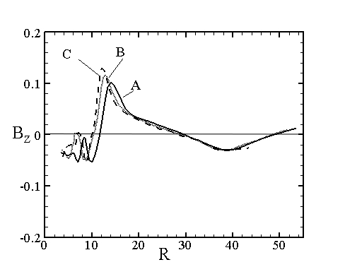
Figure 17: Radial dependences of $B_{Z}(R,Z=0)$ for grid resolutions $(N_{\theta},N_{R})$ of $A=(31,67)$, $B=(41,87)$, and $C=(50,100)$ at $t=300$ for $\alpha_{\nu}=0.1$ and $\alpha_{\eta}=0.1$.

References

- [1] Balbus, S.A., & Hawley, J.F. 1998, Rev. Mod. Phys., 70, 1
- [2] Bisnovatyi-Kogan, G.S., & Ruzmaikin, A.A. 1976, Ap&SS, 42, 401
- [3] Bisnovatyi-Kogan, G.S. & Lovelace, R.V.E. 2007, ApJ, 667, L167
- [4] Bisnovatyi-Kogan, G.S. & Lovelace, R.V.E.,2012, ApJ, 750, 109
- [5] Guan, X., & Gammie, C.F. 2009, ApJ, 697, 1901
- [6] Guilet, J. & Ogilvie, G.I. 2012, MNRAS, 424, 2097
- [7] Guilet, J. & Ogilvie, G.I. 2013, MNRAS, 430, 822 (arXiv:1212.0855)
- [8] Lii, P., Romanova, M.M., & Lovelace, R.V.E. 2012, MNRAS, 420, 2020
- [9] Lovelace, R.V.E. 1976, Nature, 262, 649
- [10] Lovelace, R. V. E., Mehanian, C., Mobarry, C.M., & Sulkanen, M.E. 1986, ApJS, 62, 1
- [11] Lovelace, R.V.E., Li, H., Koldoba, A.V., Ustyugova, G.S., & Romanova, M.M. 2002, ApJ, 572, 445
- [12] Lovelace, R.V.E., Romanova, M.M., & Bisnovatyi-Kogan, G.S. 1995, MNRAS, 275, 244
- [13] Lovelace, R. V. E., Newman, W. I., & Romanova, M. M. 1997, ApJ, 484, 628
- [14] Lovelace, R.V.E., Romanova, M.M., & Newman, W.I. 1994, ApJ 437, 136
- [15] Lovelace, R.V.E., Rothstein, D.M., & Bisnovatyi-Kogan, G.S. 2009, ApJ, 701, 885
- [16] Lubow, S. H., Papaloizou, J. C. B., & Pringle, J. E. 1994, MNRAS, 267, 235
- [17] Lynden-Bell, D., & Boily, C. 1994, MNRAS, 267, 146
- [18] Newman, W.I., Newman, A.L., & Lovelace, R.V.E. 1992, ApJ, 392, 622
- [19] Paczyński, B., & Wiita, P. 1980, A&A, 88, 23
- [20] Pariev, V.I., Colgate, S.A., Finn J.M. 2007, ApJ 658: 129-160.
- [21] Romanova, M.M, Ustyugova, G.V., Koldoba, A.V., Chechetkin, V.M., & Lovelace, R.V.E., 1998, ApJ 500, 703
- [22] Romanova, M.M, Ustyugova, G.V., Koldoba, A.V., Chechetkin, V.M., &Lovelace, R.V.E. 2002, ApJ, 578, 420
- [23] Rothstein, D.M., & Lovelace, R.V.E. 2008, ApJ, 677, 1221
- [24] Shakura, N.I., & Sunyaev, R.A. 1973, A&A, 24, 337
- [25] Ustyugova, G.V., Lovelace, R.V.E., Romanova, M.M., Li, H., & Colgate, S.A. 2000, ApJ, 541, L21
- [26] Ustyugova, G.V., Koldoba, A.V., Romanova, M.M, & Lovelace, R.V.E., 2006, ApJ 646:304-318.
- [27] van Ballegooijen, A. A. 1989, in Accretion Disks and Magnetic Fields in Astrophysics, ed. G. Belvedere ( Dordrecht: Kluwer), 99
- [28] Wang, J.C.L., Sulkanen, M.E., & Lovelace, R.V.E. 1990, ApJ, 355, 38