A monotone scheme for high-dimensional fully nonlinear PDEs

Abstract

In this paper we propose a feasible numerical scheme for high-dimensional, fully nonlinear parabolic PDEs, which includes the quasi-linear PDE associated with a coupled FBSDE as a special case. Our paper is strongly motivated by the remarkable work Fahim, Touzi and Warin [Ann. Appl. Probab. 21 (2011) 1322–1364] and stays in the paradigm of monotone schemes initiated by Barles and Souganidis [Asymptot. Anal. 4 (1991) 271–283]. Our scheme weakens a critical constraint imposed by Fahim, Touzi and Warin (2011), especially when the generator of the PDE depends only on the diagonal terms of the Hessian matrix. Several numerical examples, up to dimension 12, are reported.

, and T1Part of the research for this paper was done when this author was visiting the University of Southern California, whose hospitality is greatly appreciated. T2Supported in part by NSF Grant DMS-10-08873.

1 Introduction

In this paper we are interested in feasible numerical schemes for the following fully nonlinear parabolic PDE on $[0,T]\times\mathbb{R}^{d}$, especially in high-dimensional cases,

$$-\partial_{t}u-G\bigl{(}t,x,u,Du,D^{2}u\bigr{)}=0;\qquad u(T,\cdot)=g(\cdot).$$ (1)

The standard numerical schemes in the PDE literature, for example, finite difference methods and finite elements methods, work only for low-dimensional problems, typically $d\leq 3$, due to the well-known curse of dimensionality. However, in many applications, especially in finance, the dimension $d$ can be higher. We thus turn to the probabilistic approach, which is less sensitive to the dimension.

In the semilinear case $G=\frac{1}{2}\operatorname{tr}[\sigma^{2}(t,x)D^{2}u]+f(t,x,u,Du)$, PDE (1) is associated to a Markovian backward SDE due to the nonlinear Feynman–Kac formula introduced by Pardoux and Peng PP . Based on the regularity results of BSDEs established by Zhang Zhang , Bouchard and Touzi BT and Zhang Zhang proposed the so called backward Euler scheme for such BSDEs and hence for the semilinear PDEs, and obtained the rate of convergence. This scheme approximates the BSDE by a sequence of conditional expectations, and several efficient numerical algorithms have been proposed to compute these conditional expectations, notably: Bouchard and Touzi BT , Gobet, Lemor and Warin GLW , Bally, Pages and Printems BPP , Bender and Denk BD and Crisan and Manolarakis CM . There have been numerous publications on the subject, and the schemes have been extended to more general BSDEs, for example, reflected BSDEs which correspond to obstacle PDEs and are appropriate for pricing and hedging American options. Typically these algorithms work for 10 or even higher-dimensional problems.

We intend to numerically solve PDE (1) in the fully nonlinear case, in particular the Hamilton–Jacobi–Bellman equations and the Bellman–Isaacs equations which are widely used in stochastic control and in stochastic differential games. We remark that this is actually one main motivation of the developments of second order BSDEs by Cheridito et al. CSTV and Soner, Touzi and Zhang STZ . Our scheme is strongly inspired by the work of Fahim, Touzi and Warin FTW . Based on the monotone scheme of Barles and Souganidis BS , Fahim, Touzi and Warin FTW extended the backward Euler scheme to fully nonlinear PDE (1). In the case that $G$ is convex in $(u,Du,D^{2}u)$, they obtained the rate of convergence by using the techniques in Krylov Krylov and Barles and Jakobsen BJ . They applied the linear regression method (see, e.g., GLW ), to compute the involved conditional expectations, and presented some numerical examples up to dimension 5. We remark that the rate of convergence has been improved recently by Tan Tan , by using purely probabilistic arguments.

There is one critical constraint in FTW though. In order to ensure the monotonicity of the backward Euler scheme, they assume the lower and upper bounds of $G_{\gamma}$, the derivative of $G$ with respect to $D^{2}u$, satisfies certain constraint. However, when the dimension is high, this constraint implies that $G_{\gamma}$ is essentially a constant, and thus PDE (1) is essentially semilinear; see (9) for more details. This is, of course, not desirable in practice.

The main contribution of this paper is to propose a new scheme so as to relax the above constraint. In FTW the involved conditional expectations are expressed in terms of Brownian motion, which is unbounded. Our first simple but important observation is that we may replace it with a bounded trinomial tree, which helps to maintain the monotonicity of the scheme. We next modify the scheme by introducing a new kernel for the Hessian approximation [see the $K_{2}(\xi)$ in (3) below], but still in the paradigm of monotone scheme. In the special case where $G_{\gamma}$ is diagonal, namely $G$ involves $D^{2}u$ only through its diagonal terms, the above constraint is removed completely. Rate of convergence of our scheme is also obtained. Several numerical examples are presented. In the low-dimensional case, our scheme is comparable to finite difference method and is superior to the simulation methods. When $G_{\gamma}$ is diagonal, our scheme works well for 12-dimensional problems.

We note that PDE (1) covers the quasi-linear PDEs as a special case, which corresponds to a coupled forward–backward SDE due to the four-step scheme of Ma, Protter and Yong MPY . There are only a few papers on numerical methods for FBSDEs, for example, Douglas, Ma and Protter DMP , Makarov Makarov , Cvitanic and Zhang CZ , Delarue and Menozzi DM , Milstein and Tretyakov MT , Bender and Zhang BZ and Ma, Shen and Zhao MSZ . Most of them deal with low-dimensional FBSDEs only, except that BZ reported a 10-dimensional numerical example. However, BZ proved the rate of convergence only for time discretization, and the convergence of the linear regression approximation is not analyzed theoretically. Our scheme works for FBSDEs as well, especially when the diffusion coefficient $\sigma$ is diagonal. A numerical example for a 12-dimensional coupled FBSDE is reported.

We have also presented a few numerical examples which violate our assumptions, and thus the scheme may not be monotone. Numerical results show that our scheme still converges. In particular, we note that our current theoretical result does not cover the $G$-expectation, a nonlinear expectation introduced by Peng Peng . We nevertheless implement our scheme for a 10-dimensional HJB equation, which corresponds to a second order BSDE and includes the $G$-expectation as a special case, and it indeed converges to the true solution. It will be very interesting to investigate the convergence of our scheme, or its variations if necessary, when the monotonicity condition is violated. We shall leave this for our future research.

Finally, we note that we have recently extended the idea of monotone schemes to the so called path dependent PDEs; see Zhang and Zhuo ZZ .

The rest of the paper is organized as follows. In Section 2 we present some preliminaries. In Section 3 we propose our scheme and prove the main convergence results. Section 4 is devoted to the study of quasi-linear PDEs and the associated coupled FBSDEs. In Section 5 we discuss how to approximate the involved conditional expectations. Finally we present several numerical examples in Section 6, up to dimension 12.

2 Preliminaries

Let $T>0$ be the terminal time, $d\geq 1$ the dimension of the state variable $x$, $\mathbb{S}^{d}$ the set of $d\times d$ symmetric matrices and $\mathbb{R}^{d\times d}_{+}$ the set of nondegenerate $d\times d$ matrices. For $\gamma,\tilde{\gamma}\in\mathbb{S}^{d}$, we say $\gamma\leq\tilde{\gamma}$ if $\tilde{\gamma}-\gamma$ is nonnegative definite. For $x,\tilde{x}\in\mathbb{R}^{d}$ and $\gamma,\tilde{\gamma}\in\mathbb{R}^{d\times d}$, denote

$$x\cdot\tilde{x} := \sum_{i=1}^{d}x_{i}\tilde{x}_{i},\qquad|x|:=\sqrt{x\cdot x}\quad\mbox{and}\quad\gamma\dvtx\tilde{\gamma}:=\operatorname{tr}\bigl{(}\gamma\tilde{\gamma}^{T}\bigr{)},\qquad|\gamma|:=\sqrt{\gamma\dvtx\gamma},$$

where ^T denotes transpose. For any $\gamma=[\gamma_{ij}]\in\mathbb{S}^{d}$, denote

$$D[\gamma]:=\mbox{the diagonal matrix whose $(i,i)$th component is $\gamma_{ii}$.}$$ (2)

It is clear that, for any $\gamma,\tilde{\gamma}\in\mathbb{S}^{d}$,

$$D[\gamma]\dvtx\tilde{\gamma}=D[\gamma]\dvtx D[\tilde{\gamma}]=\gamma\dvtx D[\tilde{\gamma}].$$ (3)

Moreover, we use the same notation ${\mathbf{0}}$ to denote the zeroes in $\mathbb{R}^{d}$ and $\mathbb{S}^{d}$.

Our objective is PDE (1), where $G\dvtx(t,x,y,z,\gamma)\in[0,T]\times\mathbb{R}^{d}\times\mathbb{R}\times\mathbb{R}^{d}\times\mathbb{S}^{d}\to\mathbb{R}$ and $g\dvtx x\in\mathbb{R}^{d}\to\mathbb{R}$. We first recall the definition of viscosity solutions: an upper (resp., lower) semicontinuous function $u$ is called a viscosity subsolution (resp., viscosity supersolution) of PDE (1) if $u(T,\cdot)\leq(\mbox{resp.},\geq)\,g(x)$ and for any $(t,x)\in[0,T)\times\mathbb{R}^{d}$ and any smooth function $\varphi$ satisfying

$$[u-\varphi](t,x)=0\geq(\mbox{resp.},\leq)\,[u-\varphi](s,y)\qquad\mbox{for all }(s,y)\in[0,T]\times\mathbb{R}^{d},$$

we have

$$\bigl{[}-\partial_{t}\varphi-G\bigl{(}\cdot,\varphi,D\varphi,D^{2}\varphi\bigr{)}\bigr{]}(t,x)\leq(\mbox{resp.},\geq)\,0.$$

For the theory of viscosity solutions, we refer to the classical references CIL and FS . We remark that Barles and Souganidis BS consider more general discontinuous viscosity solutions, which is unnecessary in our situation due to the regularities we will prove; see also FTW , Remark 2.2. We shall always assume the following standing assumptions:

Assumption 2.1.

(i) $G(\cdot,0,{\mathbf{0}},{\mathbf{0}})$ and $g$ are bounded.

(ii) $G$ is continuous in $t$, uniformly Lipschitz continuous in $(x,y,z,\gamma)$ and $g$ is uniformly Lipschitz continuous in $x$.

(iii) PDE (1) is parabolic; that is, $G$ is nondecreasing in $\gamma$.

(iv) Comparison principle for PDE (1) holds in the class of bounded viscosity solutions. That is, if $u_{1}$ and $u_{2}$ are bounded viscosity subsolution and viscosity supersolution of PDE (1), respectively, then $u_{1}\leq u_{2}$.

For notational simplicity, throughout the paper we assume further that

$$G (y,z,\gamma) G_{\gamma}$$ is differentiable in so that we can use the notation , etc.

However, we emphasize that all the results in the paper do not rely on this additional assumption. Our goal of the paper is to numerically compute the viscosity solution $u$. In their seminal work Barles and Souganidis BS proposed a monotone scheme in an abstract way and proved its convergence by using the viscosity solution approach. To be precise, for any $t\in[0,T)$ and $h\in(0,T-t)$, let $\mathbb{T}^{t}_{h}$ be an operator on the set of measurable functions $\varphi\dvtx\mathbb{R}^{d}\to\mathbb{R}$. For $n\geq 1$, denote $h:={T\over n}$, $t_{i}:=ih$, $i=0,1,\ldots,n$, and define

$$u_{h}(t_{n},\cdot):=g(\cdot),\qquad u_{h}(t,\cdot):=\mathbb{T}^{t}_{t_{i}-t}\bigl{[}u_{h}(t_{i},\cdot)\bigr{]},\qquad t\in[t_{i-1},t_{i})$$ (4)

for $i=n,\ldots,1$. The following convergence result is due to Fahim, Touzi and Warin FTW , Theorem 3.6, which is based on BS .

Theorem 2.2

Let Assumption 2.1 hold. Assume $\mathbb{T}^{t}_{h}$ satisfies the following conditions: [(iii)]

Consistency: for any $(t,x)\in[0,T)\times\mathbb{R}^{d}$ and any $\varphi\in C^{1,2}([0,T)\times\mathbb{R}^{d})$,

$$\lim_{(t^{\prime},x^{\prime},h,c)\to(t,x,0,0)}{\mathbb{T}^{t^{\prime}}_{h}[[c+\varphi](t^{\prime}+h,\cdot)](x^{\prime})-[c+\varphi](t^{\prime},x^{\prime})\over h}$$

$$\qquad=\partial_{t}\varphi(t,x)+G\bigl{(}t,x,\varphi,D\varphi,D^{2}\varphi\bigr{)}.$$

Monotonicity: $\mathbb{T}^{t}_{h}[\varphi]\leq\mathbb{T}^{t}_{h}[\psi]$ whenever $\varphi\leq\psi$.

Stability: $u_{h}$ is bounded uniformly in $h$ whenever $g$ is bounded.

Boundary condition: for any $x\in\mathbb{R}^{d}$, $\lim_{(t^{\prime},x^{\prime},h)\to(T,x,0)}u_{h}(t^{\prime},x^{\prime})=g(x)$. Then the PDE (1) has a unique bounded viscosity solution $u$, and $u_{h}$ converges to $u$ locally uniformly as $h\to 0$.

We remark that in FTW the Monotonicity condition is weakened slightly. Roughly speaking, Fahim, Touzi and Waxin FTW proposed a scheme $\overline{\mathbb{T}}^{t}_{h}$ as follows. Assume there exist $\underaccent{\bar}{\sigma},\bar{\sigma}\dvtx[0,T]\times\mathbb{R}^{d}\to\mathbb{R}^{d\times d}_{+}$ such that $\frac{1}{2}\underaccent{\bar}{a}(t,x)\leq G_{\gamma}(t,x,y,z,\gamma)\leq\frac{1}{2}\bar{a}(t,x)$, for any $(t,x,y,z,\gamma)$, where $\underaccent{\bar}{a}:=\underaccent{\bar}{\sigma}\underaccent{\bar}{\sigma}^{T}$ and $\bar{a}:=\bar{\sigma}\bar{\sigma}^{T}$. Denote

$$\overline{F}(t,x,y,z,\gamma):=G(t,x,y,z,\gamma)-\tfrac{1}{2}\underaccent{\bar{}}{a}\dvtx\gamma,$$ (5)

and define

$$\overline{\mathbb{T}}^{t}_{h}[\varphi](x):=\overline{\mathcal{D}}^{t,0}_{h}\varphi(x)+h\overline{F}\bigl{(}t,x,\overline{\mathcal{D}}^{t,0}_{h}\varphi(x),\overline{\mathcal{D}}^{t,1}_{h}\varphi(x),\overline{\mathcal{D}}^{t,2}_{h}\varphi(x)\bigr{)},$$ (6)

where, for a $d$-dimensional standard Normal random variable $N$,

$$\overline{\mathcal{D}}^{t,i}_{h}\varphi(x) := \mathbb{E}\bigl{[}\varphi(x+\sqrt{h}\underaccent{\bar}{\sigma}N)\overline{K}_{i}(N)\bigr{]},\qquad i=0,1,2,$$

$$\overline{K}_{0}(N) := 1,\qquad\overline{K}_{1}(N):={\underaccent{\bar}{\sigma}^{-T}N\over\sqrt{h}},$$ (7)

$$\overline{K}_{2}(N) := {\underaccent{\bar}{\sigma}^{-T}[NN^{T}-I_{d}]\underaccent{\bar}{\sigma}^{-1}\over h},$$

and $\underaccent{\bar}{\sigma}^{-T}:=(\underaccent{\bar}{\sigma}^{-1})^{T}$. This scheme satisfies the consistency, and the stability follows from the monotonicity. However, to ensure the monotonicity, one needs to assume $\overline{F}_{\gamma}\dvtx\underaccent{\bar}{a}^{-1}\leq 1$, see FTW , proof of Lemma 3.12. This essentially requires

$$\bigl{[}\tfrac{1}{2}\bar{a}-\tfrac{1}{2}\underaccent{\bar}{a}\bigr{]}\dvtx\underaccent{\bar}{a}^{-1}\leq 1\quad\mbox{and thus}\quad\bar{a}\dvtx\underaccent{\bar}{a}^{-1}\leq d+2.$$ (8)

In the case $\underaccent{\bar}{a}=\underaccent{\bar}{\alpha}I_{d},\bar{a}=\bar{\alpha}I_{d}$ for some scalar functions $0<\underaccent{\bar}{\alpha}\leq\bar{\alpha}$, we have

$$1\leq\bar{\alpha}/\underaccent{\bar}{\alpha}\leq 1+2/d.$$ (9)

When $d$ is large, this implies $\bar{\alpha}\approx\underaccent{\bar}{\alpha}$, and thus $G$ is essentially semilinear, which of course is not desirable in practice.

Our goal of this paper is to modify algorithm (6)–(2) so as to relax the above constraint, mainly in the case that $G_{\gamma}$ is diagonally dominant. In particular, when $G_{\gamma}$ is diagonal, we remove this constraint completely.

3 The numerical scheme

In this section we present our numerical scheme and study its convergence. Our scheme involves two functions $\sigma_{0}\dvtx[0,T]\times\mathbb{R}^{d}\to\mathbb{R}^{d\times d}_{+}$ and $p\dvtx[0,T]\times\mathbb{R}^{d}\to(0,1)$ satisfying

$$\sigma_{0} \sigma_{0}^{-1} p^{-1}$$, and are bounded. (10)

Denote

$$F(t,x,y,z,\gamma) := G(t,x,y,z,\gamma)-\tfrac{1}{2}a_{0}(t,x)\dvtx\gamma$$

$$\eqntext{\mbox{where }a_{0}:=\sigma_{0}\sigma_{0}^{T};}$$ (12)

$$\widetilde{G}_{\gamma}(t,x,y,z,\gamma) := \sigma_{0}^{-1}(t,x)G_{\gamma}(t,x,y,z,\gamma)\sigma_{0}^{-T}(t,x).$$

For notational simplicity, we will be suppressing the variables when there is no confusion. Unlike Fahim, Touzi and Waxin FTW , we emphasize that we do not require $\frac{1}{2}a_{0}\leq G_{\gamma}$. Let $(\Omega,\mathcal{F},\mathbb{P})$ be a probability space. For each $(t,x)$, let $\xi:=\xi^{t,x}$ be an $\mathbb{R}^{d}$-valued random variable such that its components $\xi_{i}$, $i=1,\ldots,d$ are independent and have the identical distribution

$$\qquad\quad\mathbb{P}\biggl{(}\xi_{i}={1\over\sqrt{p}}\biggr{)}={p\over 2},\qquad\mathbb{P}\biggl{(}\xi_{i}=-{1\over\sqrt{p}}\biggr{)}={p\over 2},\qquad\mathbb{P}(\xi_{i}=0)=1-p.$$ (13)

This implies that

$$\mathbb{E}[\xi_{i}]=\mathbb{E}\bigl{[}\xi_{i}^{3}\bigr{]}=0,\qquad\mathbb{E}\bigl{[}\xi_{i}^{2}\bigr{]}=1,\qquad\mathbb{E}\bigl{[}\xi_{i}^{4}\bigr{]}=\frac{1}{p}.$$ (14)

We now modify algorithm (6)–(2),

$$\mathbb{T}^{t}_{h}[\varphi](x) := \mathcal{D}^{t,0}_{h}\varphi(x)+hF\bigl{(}t,x,\mathcal{D}^{t,0}_{h}\varphi(x),\mathcal{D}^{t,1}_{h}\varphi(x),\mathcal{D}^{t,2}_{h}\varphi(x)\bigr{)},$$ (15)

where, recalling (2) and suppressing the variables $(t,x)$,

$$\mathcal{D}^{t,i}_{h}\varphi(x) := \mathbb{E}\bigl{[}\varphi(x+\sqrt{h}\sigma_{0}\xi)K_{i}(\xi)\bigr{]},\qquad i=0,1,2,$$

$$K_{0}(\xi) := 1,\qquad K_{1}(\xi):={\sigma_{0}^{-T}\xi\over\sqrt{h}},$$ (16)

$$K_{2}(\xi) := {\sigma_{0}^{-T}[(1-p)\xi\xi^{T}-(1-3p)D[\xi\xi^{T}]-2pI_{d}]\sigma_{0}^{-1}\over(1-p)h}.$$

One may check straightforwardly that

$$E\bigl{[}K_{1}(\xi)\bigr{]}={\mathbf{0}},\qquad E\bigl{[}K_{2}(\xi)\bigr{]}={\mathbf{0}}.$$ (17)

We recall that the approximating solution $u_{h}$ is defined by (4).

Remark 3.1.

If we assume $\frac{1}{2}a_{0}\leq G_{\gamma}$ and set $p={1\over 3}$, then our scheme is obtained by replacing the normal random variable $N$ in (2) with trinomial random variable $\xi$. This in fact has already been mentioned in FTW .

Remark 3.2.

(i) The seemingly complicated kernel $K_{2}(\xi)$ is to ensure the consistency of the scheme; see Lemma 3.3 below.

(ii) The $\sigma_{0}$ is used to construct the forward process, on which we will compute the conditional expectations. This is fundamental in Monte Carlo methods which we will use.

(iii) The introduction of $p$ allows us to obtain the monotonicity of our scheme; see Section 3.2 below. However, we should point out that the crucial property is (14). Additional freedom of parameters, for example, by replacing the trinomial tree with $5$-nomial trees, will not help to weaken the monotonicity condition Assumption 3.4 below.

(iv) An additional advantage of using trinomial tree (instead of Brownian motion) is that it is bounded, which helps to ensure the monotonicity; see the proof of Lemma 3.6 and Remark 3.9(ii) below.

3.1 Consistency

We first justify our scheme by checking its consistency.

Lemma 3.3

Under Assumption 2.1 and (10), $\mathbb{T}^{t}_{h}$ satisfies the consistency requirement in Theorem 2.2(i).

Fix $(t,x)\in[0,T)\times\mathbb{R}^{d\!}$. Let $\varphi\in C^{1,2}([0,T]\times\mathbb{R}^{d})$ and $(t^{\prime},x^{\prime},h,c)\to(t,x,0,0)$. Apply Taylor expansion to $h$: with the right-hand side taking values at $(t^{\prime},x^{\prime})$,

$$\varphi\bigl{(}t^{\prime}+h,x^{\prime}+\sqrt{h}\sigma_{0}\xi\bigr{)}$$

$$\qquad=\varphi+\partial_{t}\varphi h+\sqrt{h}D\varphi\cdot\sigma_{0}\xi+{h\over 2}D^{2}\varphi\dvtx[\sigma_{0}\xi][\sigma_{0}\xi]^{T}+o(h).$$

We emphasize that, thanks to (10), the $o(\cdot)$ in this proof is uniform in $(t^{\prime},x^{\prime},h,c)$. By (14) and the independence of $\xi_{k}$ one may check straightforwardly that

$$\mathcal{D}^{t,0}_{h}\varphi\bigl{(}t^{\prime}+h,\cdot\bigr{)}\bigl{(}x^{\prime}\bigr{)} = \varphi+\partial_{t}\varphi h+{h\over 2}D^{2}\varphi\dvtx a_{0}+o(h);$$

$$\mathcal{D}^{t,1}_{h}\varphi\bigl{(}t^{\prime}+h,\cdot\bigr{)}\bigl{(}x^{\prime}\bigr{)} = D\varphi+o(\sqrt{h}).$$

Moreover, for any $i\neq j$,

$$\mathbb{E}\bigl{[}(1-p)\xi\xi^{T}-(1-3p)D\bigl{[}\xi\xi^{T}\bigr{]}-2pI_{d}\bigr{]} = {\mathbf{0}};$$

$$\mathbb{E}\bigl{[}\xi_{i}\bigl{[}(1-p)\xi\xi^{T}-(1-3p)D\bigl{[}\xi\xi^{T}\bigr{]}-2pI_{d}\bigr{]}\bigr{]} = {\mathbf{0}};$$

$$\mathbb{E}\bigl{[}\xi_{i}^{2}\bigl{[}(1-p)\xi\xi^{T}-(1-3p)D\bigl{[}\xi\xi^{T}\bigr{]}-2pI_{d}\bigr{]}\bigr{]} = 2(1-p)\delta_{i,i};$$

$$\mathbb{E}\bigl{[}\xi_{i}\xi_{j}\bigl{[}(1-p)\xi\xi^{T}-(1-3p)D\bigl{[}\xi\xi^{T}\bigr{]}-2pI_{d}\bigr{]}\bigr{]} = (1-p)(\delta_{i,j}+\delta_{j,i}).$$

Here $\delta_{i,j}$ is the $d\times d$-matrix whose $(i,j)$th component is $1$, and all other components are $0$. Then, denoting $A=[a_{i,j}]:=\sigma_{0}^{T}D^{2}\varphi\sigma_{0}$,

$$\mathbb{E}\bigl{[}\bigl{(}D^{2}\varphi\dvtx[\sigma_{0}\xi][\sigma_{0}\xi]^{T}\bigr{)}\sigma_{0}^{-T}\bigl{[}(1-p)\xi\xi^{T}-(1-3p)D\bigl{[}\xi\xi^{T}\bigr{]}-2pI_{d}\bigr{]}\sigma_{0}^{-1}\bigr{]}$$

$$\qquad=\sigma_{0}^{-T}\mathbb{E}\bigl{[}\bigl{(}A\dvtx\xi\xi^{T}\bigr{)}\bigl{[}(1-p)\xi\xi^{T}-(1-3p)D\bigl{[}\xi\xi^{T}\bigr{]}-2pI_{d}\bigr{]}\bigr{]}\sigma_{0}^{-1}$$

$$\qquad=\sigma_{0}^{-T}\sum_{i,j=1}^{d}a_{i,j}\mathbb{E}\bigl{[}\xi_{i}\xi_{j}\bigl{[}(1-p)\xi\xi^{T}-(1-3p)D\bigl{[}\xi\xi^{T}\bigr{]}-2pI_{d}\bigr{]}\bigr{]}\sigma_{0}^{-1}$$

$$\qquad=(1-p)\sigma_{0}^{-T}\sum_{i,j=1}^{d}a_{i,j}(\delta_{i,j}+\delta_{j,i})\sigma_{0}^{-1}$$

$$\qquad=2(1-p)\sigma_{0}^{-T}A\sigma_{0}^{-1}=2(1-p)D^{2}\varphi,$$

and thus

$$\mathcal{D}^{t,2}_{h}\varphi\bigl{(}t^{\prime}+h,\cdot\bigr{)}\bigl{(}x^{\prime}\bigr{)}=D^{2}\varphi+o(1).$$ (19)

Plugging (3.1) and (19) into (15) and recalling (17), we have

$$\mathbb{T}^{t^{\prime}}_{h}\bigl{[}[c+\varphi]\bigl{(}t^{\prime}+h,\cdot\bigr{)}\bigr{]}\bigl{(}x^{\prime}\bigr{)}$$

$$\qquad=c+\varphi+\partial_{t}\varphi h+{h\over 2}D^{2}\varphi\dvtx a_{0}+o(h)$$

$$\quad\qquad{}+hF\biggl{(}t^{\prime},x^{\prime},c+\varphi+\partial_{t}\varphi h+{h\over 2}D^{2}\varphi\dvtx a_{0}+o(h),$$

$$\hskip 131.0ptD\varphi+o(\sqrt{h}),D^{2}\varphi+o(1)\biggr{)}.$$

Then, by (3),

$${1\over h}\bigl{[}\mathbb{T}^{t^{\prime}}_{h}\bigl{[}[c+\varphi]\bigl{(}t^{\prime}+h,\cdot\bigr{)}\bigr{]}\bigl{(}x^{\prime}\bigr{)}-[c+\varphi]\bigl{(}t^{\prime},x^{\prime}\bigr{)}\bigr{]}$$

$$\qquad=\partial_{t}\varphi\bigl{(}t^{\prime},x^{\prime}\bigr{)}-\frac{1}{2}o(1)\dvtx a_{0}\bigl{(}t^{\prime},x^{\prime}\bigr{)}+o(1)$$

$$\quad\qquad{}+G\biggl{(}t^{\prime},x^{\prime},c+\varphi+\partial_{t}\varphi h+{h\over 2}D^{2}\varphi\dvtx a_{0}+o(h),$$

$$\hskip 125.0ptD\varphi+o(\sqrt{h}),D^{2}\varphi+o(1)\biggr{)}.$$

Sending $(t^{\prime},x^{\prime},h,c)\to(t,x,0,0)$, we obtain the consistency immediately.

3.2 The monotonicity

To obtain the monotonicity of our scheme, we need to impose an additional assumption. Let $\sigma_{0}\dvtx[0,T]\times\mathbb{R}^{d}\to\mathbb{R}^{d\times d}_{+}$ and $\widetilde{G}_{\gamma}$, $D[\widetilde{G}_{\gamma}]$ be defined by (3) and (2). Introduce the following scalar functions associated to $\sigma_{0}$:

$$\qquad\underaccent{\bar}{\alpha}(t,x) := \sup\bigl{\{}\alpha>0\dvtx\alpha I_{d}\leq D[\widetilde{G}_{\gamma}](t,x,y,z,\gamma),\ \forall(y,z,\gamma)\bigr{\}};$$

$$\bar{\alpha}(t,x) := \inf\bigl{\{}\alpha>0\dvtx\alpha I_{d}\geq D[\widetilde{G}_{\gamma}](t,x,y,z,\gamma),\ \forall(y,z,\gamma)\bigr{\}};$$

$$\Lambda(t,x) := {\bar{\alpha}(t,x)\over\underaccent{\bar}{\alpha}(t,x)},\qquad\theta(t,x):=\inf\bigl{\{}\theta\geq 0\dvtx D[\widetilde{G}_{\gamma}]\leq(1+\theta)\widetilde{G}_{\gamma}\bigr{\}};$$

$$\alpha_{p} := {p(2+3\theta)-\theta\over p(1+\theta)},\qquad c_{p}:=\sqrt{2p\Lambda+\alpha_{p}-2p};$$

$$\lambda_{p} := \sqrt{p}\biggl{[}(1-p+pd)c_{p}-{2pd\Lambda\over c_{p}}\biggr{]}{\sqrt{\underaccent{\bar}{\alpha}}\over|\sigma_{0}^{-1}|};$$

$$\lambda^{*} := \inf_{(t,x)\in[0,T]\times\mathbb{R}^{d}}\sup_{p\in[{\theta/(2(1+\theta))},{1/3}]\cap(0,{1/3}]}\lambda_{p}(t,x).$$

We remark that if we rescale $\sigma_{0}$ by a constant $c$, then $\underaccent{\bar}{\alpha}$ and $\bar{\alpha}$ will be rescaled by $c^{-2}$. However, $\Lambda$, $\theta$, $\alpha_{p}$, $c_{p}$, $\lambda_{p}$ and $\lambda^{*}$ are all invariant. The following assumption is crucial.

Assumption 3.4.

There exist $\sigma_{0}$ and $p$ satisfying (10) and: [(ii)]

$\theta(t,x)\leq 2$ for all $(t,x)$ and $\lambda^{*}>0$;

$p\in[{\theta\over 2(1+\theta)},{1\over 3}]\cap(0,{1\over 3}]$, $\lambda_{p}\geq{\lambda^{*}\over 2}$ and $\underaccent{\bar}{\alpha}=c_{p}^{-2}$.

This assumption is somewhat complicated. We shall provide several remarks concerning it after proving the monotonicity of our scheme. At below we first explain our choices of parameters which will be used in the proof of next lemma.

Remark 3.5.

(i) We need $p\leq{1\over 3}$ so that $1-3p$, the coefficient of $D[\xi\xi^{T}]$, is nonnegative. For $0\leq\theta\leq 2$, we have ${\theta\over 2(1+\theta)}\leq{1\over 3}$. Moreover, for $p\in[{\theta\over 2(1+\theta)},\break{1\over 3}]\cap(0,{1\over 3}]$, it holds that $\alpha_{p}\geq 2p$.

(ii) To ensure the monotonicity, we shall first choose $\sigma_{0}^{\prime}$ with $|\sigma_{0}^{\prime}|=1$ satisfying Assumption 3.4, preferably the one maximizing the corresponding $\lambda^{*}$. We next choose $p\in[{\theta\over 2(1+\theta)},{1\over 3}]\cap(0,{1\over 3}]$ such that $\lambda_{p}\geq{\lambda^{*}\over 2}$. Finally we rescale $\sigma_{0}^{\prime}$ to obtain $\sigma_{0}$ satisfying $\underaccent{\bar}{\alpha}=c_{p}^{-2}$.

(iii) The above choices of $p$ and $\sigma_{0}$ is somewhat optimal in order to maintain the monotonicity. However, given $G$, they may not be optimal for the convergence of the scheme. For example, a smaller $p$ may help for the monotonicity, but may increase the variance of the Monte Carlo simulation which will be introduced later. In our numerical examples in Section 6 below, we may choose them slightly differently. It is not clear to us how to choose $p$ and $\sigma_{0}$ so as to optimize the overall efficiency of the algorithm.

Lemma 3.6

Let Assumptions 2.1 and 3.4 hold, and consider the algorithm by using the $p$ and $\sigma_{0}$ as specified in Remark 3.5(ii). Then there exists a constant $h_{0}>0$, depending on $d,T,\lambda^{*}$, and the bounds and Lipschitz constants in Assumption 2.1 and (10), such that $\mathbb{T}^{t}_{h}$ satisfies the monotonicity in Theorem 2.2(ii) for all $h\in(0,h_{0}]$.

Let $\varphi_{1}\leq\varphi_{2}$ be bounded and $\psi:=\varphi_{2}-\varphi_{1}\geq 0$. Then by (15) we have, at $(t,x)$,

$$\qquad\mathbb{T}^{t}_{h}[\varphi_{2}]-\mathbb{T}^{t}_{h}[\varphi_{1}]=\mathcal{D}^{t,0}_{h}\psi+h\bigl{[}F_{y}\mathcal{D}^{t,0}_{h}\psi+F_{z}\cdot\mathcal{D}^{t,1}_{h}\psi+F_{\gamma}\dvtx\mathcal{D}^{t,2}_{h}\psi\bigr{]}.$$ (21)

Here the terms $F_{y},F_{z},F_{\gamma}$ are defined in an obvious way, and we emphasize that they are deterministic. Plug (3) into the above equality, then

$$\mathbb{T}^{t}_{h}[\varphi_{2}]-\mathbb{T}^{t}_{h}[\varphi_{1}]$$

$$\qquad=\mathbb{E}[\psi(x+\sqrt{h}\sigma_{0}\xi)\bigl{[}1+h\bigl{[}F_{y}+F_{z}\cdot K_{1}(\xi)+F_{\gamma}\dvtx K_{2}(\xi)\bigr{]}\bigr{]}$$ (22)

$$\qquad=\mathbb{E}\biggl{[}\psi(x+\sqrt{h}\sigma_{0}\xi)\biggl{[}1+hF_{y}+\sqrt{h}F_{z}\cdot\bigl{(}\sigma_{0}^{-T}\xi\bigr{)}+{I\over 1-p}\biggr{]}\biggr{]},$$

where

$$I := F_{\gamma}\dvtx\bigl{(}\sigma_{0}^{-T}\bigl{[}(1-p)\xi\xi^{T}-(1-3p)D\bigl{[}\xi\xi^{T}\bigr{]}-2pI_{d}\bigr{]}\sigma_{0}^{-1}\bigr{)}$$

$$= \bigl{[}\widetilde{G}_{\gamma}-\tfrac{1}{2}I_{d}\bigr{]}\dvtx\bigl{[}(1-p)\xi\xi^{T}-(1-3p)D\bigl{[}\xi\xi^{T}\bigr{]}-2pI_{d}\bigr{]}$$

$$= (1-p)\bigl{[}\widetilde{G}_{\gamma}-\tfrac{1}{2}I_{d}\bigr{]}\dvtx\bigl{(}\xi\xi^{T}\bigr{)}-(1-3p)\bigl{[}D[\widetilde{G}_{\gamma}]-\tfrac{1}{2}I_{d}\bigr{]}\dvtx\bigl{(}\xi\xi^{T}\bigr{)}$$

$${}-2p\operatorname{tr}(\widetilde{G}_{\gamma})+pd.$$

Denote $\alpha_{i}:=(\widetilde{G}_{\gamma})_{ii}$. Then it follows from the definition of $\theta$ that

$$I \geq (1-p)\biggl{[}{1\over 1+\theta}D[\widetilde{G}_{\gamma}]-\frac{1}{2}I_{d}\biggr{]}\dvtx\bigl{(}\xi\xi^{T}\bigr{)}-(1-3p)\biggl{[}D[\widetilde{G}_{\gamma}]-\frac{1}{2}I_{d}\biggr{]}\dvtx\bigl{(}\xi\xi^{T}\bigr{)}$$

$${}-2p\operatorname{tr}(\widetilde{G}_{\gamma})+pd$$

$$= p\alpha_{p}D[\widetilde{G}_{\gamma}]\dvtx\bigl{(}\xi\xi^{T}\bigr{)}-p|\xi|^{2}-2p\operatorname{tr}(\widetilde{G}_{\gamma})+pd$$

$$= pd-p\sum_{i=1}^{d}\bigl{[}\xi_{i}^{2}+2\alpha_{i}-\alpha_{p}\alpha_{i}\xi_{i}^{2}\bigr{]}.$$

Note that $\underaccent{\bar}{\alpha}\leq\alpha_{i}\leq\bar{\alpha}$, $\alpha_{p}\geq 2p$ by Remark 3.5(i), $\underaccent{\bar}{\alpha}=c_{p}^{-2}$ by Remark 3.5(ii) and $\xi_{i}^{2}$ takes only values $0$ and ${1\over p}$. Then

$$p\bigl{[}\xi_{i}^{2}+2\alpha_{i}-\alpha_{p}\alpha_{i}\xi_{i}^{2}\bigr{]} \leq (2p\alpha_{i})\vee\bigl{[}1-(\alpha_{p}-2p)\alpha_{i}\bigr{]}$$

$$\leq {2p\bar{\alpha}}\vee\bigl{[}1-(\alpha_{p}-2p)\underaccent{\bar}{\alpha}\bigr{]}=2p\bar{\alpha}=2p\Lambda c_{p}^{-2}.$$

Thus

$$1-p+I \geq 1-p+pd-2pd\Lambda c_{p}^{-2}={\lambda_{p}|\sigma_{0}^{-1}|\over\sqrt{p}}\geq{\lambda^{*}|\sigma_{0}^{-1}|\over 2\sqrt{p}}.$$ (23)

By the Lipschitz continuity of $G$ in $\gamma$, we have

$$C\bigl{|}\sigma_{0}^{-1}\bigr{|}^{2}\geq\bar{\alpha}=\Lambda c_{p}^{-2}={\Lambda\over 2p\Lambda+\alpha_{p}-2p}\geq{1\over\alpha_{p}}\geq{1\over 3}.$$ (24)

Note that $p\leq{1\over 3}$ and $|\xi_{i}|$ takes values $0$ or ${1\over\sqrt{p}}$. Then

$$\bigl{|}hF_{y}+\sqrt{h}F_{z}\cdot\bigl{(}\sigma_{0}^{-1}\xi\bigr{)}\bigr{|}\leq Ch+{C\sqrt{h}\over\sqrt{p}}\bigl{|}\sigma_{0}^{-1}\bigr{|}\leq{C_{1}\sqrt{h_{0}}\over\sqrt{p}}\bigl{|}\sigma_{0}^{-1}\bigr{|},$$ (25)

for some constant $C_{1}$. Set $h_{0}:=({3\lambda^{*}\over 4C_{1}})^{2}$, and recall again that $p\leq{1\over 3}$ and (10). Plugging (23) and (25) into (3.2), we see that

$$1+hF_{y}+\sqrt{h}F_{z}\cdot\bigl{(}\sigma_{0}^{-1}\xi\bigr{)}+{I\over 1-p}\geq 0$$

and thus proves the monotonicity.

We remark that our algorithm works well when $\widetilde{G}_{\gamma}$ is diagonally dominated, namely when $\theta$ is uniformly small. In this case, we have the following simple sufficient condition for Assumption 3.4.

Proposition 3.7

Let Assumption 2.1 hold. Assume there exist $\sigma_{0}\dvtx\break[0,T]\times\mathbb{R}^{d}\to\mathbb{R}^{d\times d}_{+}$ and a small constant $\varepsilon_{0}>0$ such that $\sigma_{0}$ and $\sigma_{0}^{-1}$ are bounded and, for the $C_{0}$ in (24),

$$\theta\leq{\varepsilon_{0}\over 4dC_{0}}\quad\mbox{and}\quad{\underaccent{\bar}{\alpha}(t,x)\over|\sigma_{0}^{-1}|^{2}}\geq\varepsilon_{0}.$$ (26)

Then Assumption 3.4 holds, and consequently $\mathbb{T}^{t}_{h}$ is monotone.

First, set $p:={\varepsilon_{0}\over 4dC_{0}}\in[{\theta\over 2(1+\theta)},{1\over 3}]\cap(0,{1\over 3}]$. It is clear that (10) holds. By the first inequality of (24) and second inequality of (26), we have $\Lambda\leq{C_{0}\over\varepsilon_{0}}$. Then $\alpha_{p}\geq{p(1+3\theta)\over p(1+\theta)}\geq 1$, $c_{p}\geq\sqrt{\alpha_{p}}\geq 1$, and thus,

$$\lambda_{p}\geq\sqrt{p}\biggl{[}1-p+pd-2pd{C_{0}\over\varepsilon_{0}}\biggr{]}\varepsilon_{0}\geq\sqrt{\varepsilon_{0}\over 4dC_{0}}\frac{1}{2}\varepsilon_{0}={\varepsilon_{0}^{3/2}\over C}.$$

This implies Assumption 3.4 immediately.

Remark 3.8.

In this remark we investigate the bound of $\Lambda$ for our algorithm, and compare it with (9). [(iii)]

When $\widetilde{G}_{\gamma}$ is diagonally dominated, in particular when $\theta=0$, under (26) we remove the constraint (9) completely and thus improve the result of FTW significantly. We also note that when $d=1$ we always have $\theta=0$ and thus the bound constraint does not exist in our case.

Let $0<\theta\leq 2$ and $d\geq 2$. For simplicity, we shall assume $\underaccent{\bar}{\alpha},\bar{\alpha}$ and $\theta$ are all constants. Note that

$$\lambda_{p} = {\sqrt{p\underaccent{\bar}{\alpha}}\over c_{p}|\sigma_{0}^{-1}|}\bigl{[}(1-p+pd)(2p\Lambda+\alpha_{p}-2p)-2pd\Lambda\bigr{]}$$

$$= 2p(1-p)\sqrt{p}(d-1){\sqrt{p\underaccent{\bar}{\alpha}}\over c_{p}|\sigma_{0}^{-1}|}\biggl{[}{(1-p+pd)(\alpha_{p}-2p)\over 2p(1-p)(d-1)}-\Lambda\biggr{]}$$

$$= 2p(1-p)(d-1){\sqrt{p\underaccent{\bar}{\alpha}}\over c_{p}|\sigma_{0}^{-1}|}\biggl{[}\biggl{[}1+{1\over(d-1)p}\biggr{]}\biggl{[}1-{\theta\over 2(1+\theta)p}\biggr{]}-\Lambda\biggr{]}.$$

Then our constraint is

$$\Lambda<\Lambda_{\theta}:=\sup_{p\in[{\theta/(2(1+\theta))},{1/3}]}\biggl{[}1+{1\over(d-1)p}\biggr{]}\biggl{[}1-{\theta\over 2(1+\theta)p}\biggr{]}.$$ (27)

When $0<\theta\leq{2\over d+3}$, one may compute straightforwardly that the optimal $p:={2\theta\over 2-(d-3)\theta}\in[{\theta\over 2(1+\theta)},{1\over 3}]$ and thus $\Lambda_{\theta}=1+{[2-(d-3)\theta]^{2}\over 8\theta(1+\theta)(d-1)}$. Once again, we see that $\Lambda_{\theta}$ is large when $\theta$ is small. In particular, there exists unique $\theta_{d}\leq{2\over d+3}$ such that $\Lambda_{\theta_{d}}=1+{2\over d}$. Therefore, when $\theta<\theta_{d}$, our scheme allows for a larger bound of $\Lambda$ than (9).

When $\theta\geq{2\over d+3}$, or more generally when $\theta\geq\theta_{d}$, we may set $p:={1\over 3}$ and our algorithm reduces back to FTW , by replacing the Brownian motion with trinomial tree; see Remark 3.1. In this case Assumption 3.4 may be violated, but we can still easily obtain the same bound (8) as in FTW . That is, under (8) our algorithm (with $p={1\over 3}$) is still monotone, but the proof should follow the arguments in FTW , rather than those in Lemma 3.6.

By (27), to maintain monotonicity it suffices to choose $p$ such that $[1+{1\over(d-1)p}][1-{\theta\over 2(1+\theta)p}]\geq\Lambda$. In particular, when $\theta=0$, one natural choice is

$$p:=\min\biggl{(}{1\over(\Lambda-1)(d-1)},{1\over 3}\biggr{)}.$$

We remark further that, in light of Remark 3.5(iii), we may not want to choose smaller $p$ although it also maintains the monotonicity.

Remark 3.9.

This remark concerns the degeneracy of $G$. [(iii)]

The second inequality of (26) implies immediately the uniform nondegeneracy of $G_{\gamma}$: $D[\sigma_{0}^{-1}G_{\gamma}\sigma_{0}^{-T}]\geq\varepsilon_{0}|\sigma_{0}^{-1}|^{2}I_{d}$. This is mainly due to the term $F_{z}\cdot(\sigma_{0}^{-1}\xi)$ in (3.2). In FTW , $G_{\gamma}$ is assumed to be nondegenerate, but not necessarily uniformly, under the additional assumption that $F_{z}^{T}F_{\gamma}^{-1}F_{z}$ is bounded ($F_{\gamma}$ is nondegenerate in FTW ). If we assume that $|F_{z}|\leq C|\underaccent{\bar}{\alpha}|$, then following similar arguments, in particular by using a weaker version of monotonicity in the spirit of FTW , Lemma 3.12, we may remove the uniform nondegeneracy in (26) as well.

Unlike FTW , we do not require $G_{\gamma}\geq\frac{1}{2}a_{0}$ and thus $F$ can be degenerate. This is possible mainly because we use a bounded trinomial tree instead of an unbounded Brownian motion.

When $G$ is degenerate, namely $\underaccent{\bar}{\alpha}$ can be equal to $0$, one can approximate the generator $G$ by $G^{\varepsilon}:=G+\varepsilon I_{d}\dvtx\gamma$ and numerically solve the corresponding solution $u^{\varepsilon}$. By the stability of viscosity solutions we see that $u^{\varepsilon}$ converges to $u$ locally uniformly.

Motivated from pricing Asian options, in a recent work Tan Tan2 investigated the numerical approximation for the following type of PDE with solution $u(t,x,y)$:

$$-\partial_{t}u(t,x,y)-G\bigl{(}t,x,y,u,D_{x}u,D_{xx}^{2}u\bigr{)}-H(t,x,y,u,D_{x}u,D_{y}u)=0,$$

where $G$ is nondegenerate in $D^{2}_{xx}u$, but the PDE is always degenerate in $D^{2}_{yy}u$.

3.3 Stability

Given the monotonicity, one may prove stability following standard arguments.

Lemma 3.10

Let Assumptions 2.1 and 3.4 hold. Then for any $h\in(0,h_{0}]$, $\mathbb{T}^{t}_{h}$ satisfies the stability in Theorem 2.2(iii).

First, it follows from Lemma 3.6 that $\mathbb{T}^{t}_{h}$ satisfies the monotonicity. Denote $C_{n}:=\sup_{x\in\mathbb{R}^{d}}|u_{h}(t_{n},x)|$ and $C_{i}:=\sup_{(t,x)\in[t_{i},t_{i+1})\times\mathbb{R}^{d}}|u_{h}(t,\break x)|$, $i=n-1,\ldots,0$. Since $g$ is bounded, we see that $C_{n}\leq C$. We claim that

$$C_{i}\leq(1+Ch)C_{i+1}+Ch.$$ (28)

Then by the discrete Gronwall inequality, we see that

$$\max_{0\leq i\leq n-1}C_{i}\leq C(1+Ch)^{n}[C_{n}+nh]\leq C.$$

This proves the lemma.

We now prove (28). Let $(t,x)\in[t_{i},t_{i+1})\times\mathbb{R}^{d}$ and denote $h^{\prime}:=t_{i}-t\leq h$, $\xi:=\xi^{t,x}$. Similar to (21), one may easily get

$$u_{h}(t,x) = \mathbb{E}\bigl{[}u_{h}\bigl{(}t_{i+1},x+\sqrt{h^{\prime}}\sigma_{0}\xi\bigr{)}I_{i+1}\bigr{]}+h^{\prime}F(t_{i},x,0,{\mathbf{0}},{\mathbf{0}}),$$ (29)

where, for some deterministic $F_{y}(t_{i}),F_{z}(t_{i}),F_{\gamma}(t_{i})$ defined in an obvious way,

$$I_{i+1} := 1+h^{\prime}\bigl{[}F_{y}(t_{i})+F_{z}(t_{i})\cdot K_{1}(\xi)+F_{\gamma}(t_{i})\dvtx K_{2}(\xi)\bigr{]}.$$

The monotonicity in Lemma 3.6 exactly means $I_{i+1}\geq 0$. Noting that $F(t_{i},x,\break 0,{\mathbf{0}},{\mathbf{0}})=G(t_{i},x,0,{\mathbf{0}},{\mathbf{0}})$ is bounded, then

$$\bigl{|}u_{h}(t,x)\bigr{|} \leq \mathbb{E}\bigl{[}\bigl{|}u_{h}\bigl{(}t_{i+1},x+\sqrt{h^{\prime}}\sigma_{0}\xi\bigr{)}\bigr{|}I_{i+1}\bigr{]}+Ch^{\prime}\leq C_{i+1}\mathbb{E}[I_{i+1}]+Ch^{\prime}.$$

By (17), we see that $E_{t_{i}}[I_{i+1}]=1+h^{\prime}F_{y}(t_{i})\leq 1+Ch^{\prime}$. Then

$$\bigl{|}u_{h}(t,x)\bigr{|} \leq \bigl{(}1+Ch^{\prime}\bigr{)}C_{i+1}+Ch^{\prime}\leq(1+Ch)C_{i+1}+Ch.$$

Since $(t,x)$ is arbitrary, we obtain (28).

3.4 Boundary condition

Lemma 3.11

Let Assumptions 2.1 and 3.4 hold, then

$$\bigl{|}u_{h}(t,x)-g(x)\bigr{|}\leq C(T-t)^{1/2}.$$

Without loss of generality, we assume $t=t_{k}$ for some $k$. Fix $(t_{k},x)$, and denote $X^{n}_{t_{k}}:=x$, $\mathcal{F}^{n}_{t_{k}}:=\{\varnothing,\Omega\}$. For $j=k+1,\ldots,n$, define recursively

$$X^{n}_{t_{j}}:=X^{n}_{t_{j-1}}+\sqrt{h}\sigma_{0}\bigl{(}t_{j-1},X^{n}_{t_{j-1}}\bigr{)}\xi^{j},\qquad\mathcal{F}^{n}_{t_{j}}:=\mathcal{F}^{n}_{t_{j-1}}\vee\sigma\bigl{(}\xi^{j}\bigr{)},$$

where $\xi^{j}:=\xi^{t_{j-1},X^{n}_{t_{j-1}}}$ is determined by (13) and is independent of $\mathcal{F}^{n}_{t_{j-1}}$. Then it is clear,

$$u_{h}\bigl{(}t_{j-1},X^{n}_{t_{j-1}}\bigr{)} = \mathbb{E}_{t_{j-1}}\bigl{[}u_{h}\bigl{(}t_{j},X^{n}_{t_{j}}\bigr{)}\bigr{]}$$

$${}+hF\bigl{(}t_{j-1},X^{n}_{t_{j-1}},\mathbb{E}_{t_{j-1}}\bigl{[}u_{h}\bigl{(}t_{j},X^{n}_{t_{j}}\bigr{)}\bigr{]},$$

$$\hskip 32.0pt\mathbb{E}_{t_{j-1}}\bigl{[}u_{h}\bigl{(}t_{j},X^{n}_{t_{j}}\bigr{)}K_{1}\bigl{(}\xi^{j}\bigr{)}\bigr{]},\mathbb{E}_{t_{j-1}}\bigl{[}u_{h}\bigl{(}t_{j},X^{n}_{t_{j}}\bigr{)}K_{2}\bigl{(}\xi^{j}\bigr{)}\bigr{]}\bigr{)}.$$

Similar to the proof of Lemma 3.10, we have

$$u_{h}\bigl{(}t_{j-1},X^{n}_{t_{j-1}}\bigr{)} = \mathbb{E}_{t_{j-1}}\bigl{[}u_{h}\bigl{(}t_{j},X^{n}_{t_{j}}\bigr{)}I_{j}\bigr{]}+hF\bigl{(}t_{j-1},X^{n}_{t_{j-1}},0,{\mathbf{0}},{\mathbf{0}}\bigr{)},$$

where, by abusing the notation $I$ slightly,

$$I_{j} := 1+h\bigl{[}F_{y}(t_{j-1})+F_{z}(t_{j-1})\cdot K_{1}\bigl{(}\xi^{j}\bigr{)}+F_{\gamma}(t_{j-1})\dvtx K_{2}\bigl{(}\xi^{j}\bigr{)}\bigr{]}\geq 0,$$

and $F_{y}(t_{j-1}),F_{z}(t_{j-1}),F_{\gamma}(t_{j-1})$ are defined in an obvious way. Denote

$$J_{k}:=1\quad\mbox{and}\quad J_{i}:=\prod_{j=k+1}^{i}I_{j},\qquad i=k+1,\ldots,n.$$

Recalling $u_{h}(t_{n},x)=g(x)$, by induction we get

$$u_{h}(t_{k},x)=u_{h}\bigl{(}t_{k},X^{n}_{t_{k}}\bigr{)}=\mathbb{E}\Biggl{[}g\bigl{(}X^{n}_{t_{n}}\bigr{)}J_{n}+h\sum_{j=k}^{n-1}J_{j}F\bigl{(}t_{j},X^{n}_{t_{j}},0,{\mathbf{0}},{\mathbf{0}}\bigr{)}\Biggr{]}.$$

Since $g$ is bounded and uniformly Lipschitz continuous, we may let $g_{\epsilon}$ be a standard smooth molifier of $g$ such that

$$\|g_{\epsilon}-g\|_{\infty}\leq C\epsilon,\qquad\|Dg_{\epsilon}\|_{\infty}\leq C\quad\mbox{and}\quad\bigl{\|}D^{2}g_{\epsilon}\bigr{\|}_{\infty}\leq C\epsilon^{-1}.$$ (30)

Then, noting again that $F(t,x,0,{\mathbf{0}},{\mathbf{0}})=G(t,x,0,{\mathbf{0}},{\mathbf{0}})$ is bounded,

$$\bigl{|}u_{h}(t_{k},x)-g(x)\bigr{|}$$

$$\qquad\leq\bigl{|}\mathbb{E}\bigl{[}g_{\varepsilon}\bigl{(}X^{n}_{t_{n}}\bigr{)}J_{n}\bigr{]}-g_{\varepsilon}(x)\bigr{|}+C\varepsilon\mathbb{E}[J_{n}]+Ch\mathbb{E}\Biggl{[}\sum_{j=k}^{n-1}J_{j}\Biggr{]}+C\varepsilon$$

$$\qquad=\Biggl{|}\sum_{i=k+1}^{n}\mathbb{E}\bigl{[}g_{\varepsilon}\bigl{(}X^{n}_{t_{i}}\bigr{)}J_{i}-g_{\varepsilon}\bigl{(}X^{n}_{t_{i-1}}\bigr{)}J_{i-1}\bigr{]}\Biggr{|}+C\varepsilon\mathbb{E}[J_{n}]+Ch\mathbb{E}\Biggl{[}\sum_{j=k}^{n}J_{j}\Biggr{]}+C\varepsilon$$

$$\qquad=\Biggl{|}\sum_{i=k+1}^{n}\mathbb{E}\bigl{[}\bigl{[}g_{\varepsilon}\bigl{(}X^{n}_{t_{i}}\bigr{)}-g_{\varepsilon}\bigl{(}X^{n}_{t_{i-1}}\bigr{)}\bigr{]}J_{i}+g_{\varepsilon}\bigl{(}X^{n}_{t_{i-1}}\bigr{)}J_{i-1}[I_{i}-1]\bigr{]}\Biggr{|}$$

$$\quad\qquad{}+C\varepsilon\mathbb{E}[J_{n}]+Ch\mathbb{E}\Biggl{[}\sum_{j=k}^{n-1}J_{j}\Biggr{]}+C\varepsilon.$$

Since $\mathbb{E}_{t_{j-1}}[I_{j}]=1+hF_{y}(t_{j-1})$, we have

$$\bigl{|}\mathbb{E}_{t_{i-1}}[I_{i}]-1\bigr{|}\leq Ch\quad\mbox{and}\quad\mathbb{E}[J_{i}]\leq(1+Ch)^{i-k}\leq C.$$ (31)

Thus

$$\bigl{|}u_{h}(t_{k},x)-g(x)\bigr{|}$$

(32)

$$\qquad\leq\Biggl{|}\sum_{i=k+1}^{n}\mathbb{E}\bigl{[}\bigl{[}g_{\varepsilon}\bigl{(}X^{n}_{t_{i}}\bigr{)}-g_{\varepsilon}\bigl{(}X^{n}_{t_{i-1}}\bigr{)}\bigr{]}J_{i}\bigr{]}\Biggr{|}+C(n-k)h+C\varepsilon.$$

Moreover, for some appropriate $\mathcal{F}_{t_{i}}$-measurable $\widetilde{X}^{n}_{t_{i}}$,

$$g_{\varepsilon}\bigl{(}X^{n}_{t_{i}}\bigr{)}-g_{\varepsilon}\bigl{(}X^{n}_{t_{i-1}}\bigr{)} = \sqrt{h}Dg_{\epsilon}\bigl{(}X^{n}_{t_{i-1}}\bigr{)}\cdot\sigma_{0}\xi^{i}+{h\over 2}D^{2}g_{\epsilon}\bigl{(}\widetilde{X}^{n}_{t_{i}}\bigr{)}\dvtx\bigl{(}\sigma_{0}\xi^{i}\bigr{)}\bigl{(}\sigma_{0}\xi^{i}\bigr{)}^{T}.$$

By (10), we have

$$\bigl{|}\mathbb{E}_{t_{i-1}}\bigl{[}Dg_{\epsilon}\bigl{(}X^{n}_{t_{i-1}}\bigr{)}\cdot\sigma_{0}\xi^{i}I_{i}\bigr{]}\bigr{|}$$

$$\qquad=\bigl{|}\mathbb{E}_{t_{i-1}}\bigl{[}h\bigl{[}Dg_{\epsilon}\bigl{(}X^{n}_{t_{i-1}}\bigr{)}\cdot\sigma_{0}\xi^{i}\bigr{]}\bigl{[}F_{z}(t_{i-1})\cdot K_{1}\bigl{(}\xi^{i}\bigr{)}\bigr{]}\bigr{]}\bigr{|}\leq C\sqrt{h};$$

$$\bigl{|}\mathbb{E}_{t_{i-1}}\bigl{[}D^{2}g_{\epsilon}\bigl{(}\widetilde{X}^{n}_{t_{i}}\bigr{)}\dvtx\bigl{(}\sigma_{0}\xi^{i}\bigr{)}\bigl{(}\sigma_{0}\xi^{i}\bigr{)}^{T}I_{i}\bigr{]}\bigr{|}\leq C\varepsilon^{-1}\mathbb{E}_{t_{i-1}}[I_{i}]\leq C\varepsilon^{-1}.$$

Then

$$\bigl{|}\mathbb{E}_{t_{i-1}}\bigl{[}\bigl{[}g_{\varepsilon}\bigl{(}X^{n}_{t_{i}}\bigr{)}-g_{\varepsilon}\bigl{(}X^{n}_{t_{i-1}}\bigr{)}\bigr{]}I_{i}\bigr{]}\bigr{|}\leq Ch\bigl{[}1+\varepsilon^{-1}\bigr{]}.$$

Plugging this into (3.4) and recalling (31), we have

$$\bigl{|}u_{h}(t_{k},x)-g(x)\bigr{|} \leq C(n-k)h\bigl{[}1+\varepsilon^{-1}\bigr{]}+C\varepsilon.$$

Note that $(n-k)h=T-t_{k}$. Setting $\varepsilon:=\sqrt{T-t_{k}}$, we obtain the result.

3.5 Convergence results

First, combine Lemmas 3.3, 3.6, 3.10, 3.11, and immediately from Theorem 2.2, we have the following:

Theorem 3.12

Let Assumptions 2.1 and 3.4 hold. Then the PDE (1) has a unique bounded viscosity solution $u$, and $u_{h}$ converges to $u$ locally uniformly as $h\to 0$.

We next study the rate of convergence. We first consider the case that $u$ is smooth. Let $C^{[2]}_{b}([0,T]\times\mathbb{R}^{d})$ denote the subset of $C^{1,2}([0,T]\times\mathbb{R}^{d})$ such that $u$, $\partial_{t}u,Du,D^{2}u$ are bounded; and $C^{[4]}_{b}([0,T]\times\mathbb{R}^{d})$ the set of $u\in C^{[2]}_{b}([0,T]\times\mathbb{R}^{d})$ such that each component of $\partial_{t}u,Du,D^{2}u$ is also in $C^{[2]}_{b}([0,T]\times\mathbb{R}^{d})$.

Theorem 3.13

Let Assumptions 2.1 and 3.4 hold and $h\in(0,h_{0})$. Assume further that $u\in C_{b}^{[4]}([0,T]\times\mathbb{R}^{d})$, and $G$ is locally uniformly Lipschitz continuous in $x$, locally uniformly on $(y,z,\gamma)$. Then there exists a constant $C$, independent of $h$ (or $n$), such that

$$\bigl{|}u_{h}(t,x)-u(t,x)\bigr{|} \leq Ch\qquad\mbox{for all }(t,x).$$

Again, since $h<h_{0}$, it follows from Lemma 3.6 that $\mathbb{T}^{t}_{h}$ satisfies the monotonicity. Denote $C_{n}:=\sup_{x\in\mathbb{R}^{d}}|u_{h}(t_{n},x)-u(t_{n},x)|$ and $C_{i}:=\sup_{(t,x)\in[t_{i},t_{i+1})\times\mathbb{R}^{d}}|u_{h}(t,x)-u(t,x)|$, $i=n-1,\ldots,0$. We claim that

$$C_{i}\leq(1+Ch)C_{i+1}+Ch^{2}.$$ (33)

Since $C_{n}=0$, then by the discrete Gronwall inequality, we see that

$$\max_{0\leq i\leq n-1}C_{i}\leq C(1+Ch)^{n}\bigl{[}C_{n}+nh^{2}\bigr{]}\leq Ch.$$

This proves the theorem.

We now prove (33). Similar to the proof of Lemma 3.10, we shall only estimate $|u_{h}(t_{i},x)-u(t_{i},x)|$, and the estimate for the general $|u_{h}(t,x)-u(t,x)|$ is similar. For this purpose, recall (15), (3), and define

$$\tilde{u}_{h}(t_{i},x) := \bigl{[}\mathcal{D}^{t_{i},0}u(t_{i+1},\cdot)\bigr{]}(x)$$

$${}+hF\bigl{(}t_{i},x,\bigl{[}\mathcal{D}^{t_{i},0}u(t_{i+1},\cdot)\bigr{]}(x),\bigl{[}\mathcal{D}^{t_{i},1}u(t_{i+1},\cdot)\bigr{]}(x),$$

$$\hskip 146.0pt{}\bigl{[}\mathcal{D}^{t_{i},2}u(t_{i+1},\cdot)\bigr{]}(x)\bigr{)}.$$

We note that the right-hand side of above uses the true solution $u$, instead of $u_{h}$ in (4). It is clear that

$$\qquad\bigl{|}u_{h}(t_{i},x)-u(t_{i},x)\bigr{|}\leq\bigl{|}u_{h}(t_{i},x)-\tilde{u}_{h}(t_{i},x)\bigr{|}+\bigl{|}\tilde{u}_{h}(t_{i},x)-u(t_{i},x)\bigr{|}.$$ (35)

Compare (4) and (3.5), and by the first equality of (21) we have, at $(t_{i},x)$,

$$u_{h}(t_{i},x)-\tilde{u}_{h}(t_{i},x)$$

$$\qquad=\mathbb{E}\bigl{[}[u_{h}-u](t_{i+1},x+\sqrt{h}\sigma_{0}\xi)\bigl{[}1+h\bigl{[}F_{y}+F_{z}\cdot K_{1}(\xi)+F_{\gamma}\dvtx K_{2}(\xi)\bigr{]}\bigr{]}\bigr{]}.$$

Then it follows from similar arguments in the proof of Lemma 3.10 that

$$\bigl{|}u_{h}(t_{i},x)-\tilde{u}_{h}(t_{i},x)\bigr{|}\leq(1+Ch)C_{i+1}.$$ (36)

Next, since $u\in C_{b}^{[4]}([0,T]\times\mathbb{R}^{d})$, applying Taylor expansion and by (14), one may check straightforwardly that, at $(t_{i},x)$,

$$\bigl{[}\mathcal{D}^{t_{i},0}u(t_{i+1},\cdot)\bigr{]}(x) = u+\partial_{t}uh+{h\over 2}D^{2}u\dvtx a_{0}+O\bigl{(}h^{2}\bigr{)};$$

$$\bigl{[}\mathcal{D}^{t_{i},1}u(t_{i+1},\cdot)\bigr{]}(x) = Du+O(h);\qquad\bigl{[}\mathcal{D}^{t_{i},2}u(t_{i+1},\cdot)\bigr{]}(x)=D^{2}u+O(h),$$

where $O(\cdot)$ is uniform, thanks to (10). Then, again at $(t_{i},x)$,

$$\tilde{u}_{h}-u = \partial_{t}uh+{h\over 2}D^{2}u\dvtx a_{0}+O\bigl{(}h^{2}\bigr{)}$$

$${}+hF\bigl{(}t_{i},x,u+O(h),Du+O(h),D^{2}u+O(h)\bigr{)}$$

$$= \partial_{t}uh-{h\over 2}O(h)\dvtx a_{0}+O\bigl{(}h^{2}\bigr{)}$$

$${}+hG\bigl{(}t_{i},x,u+O(h),Du+O(h),D^{2}u+O(h)\bigr{)}.$$

Note that $u$ satisfies the PDE (1), and recall (3). Then

$$\bigl{|}\tilde{u}_{h}(t_{i},x)-u(t_{i},x)\bigr{|}$$

$$\qquad=O\bigl{(}h^{2}\bigr{)}+h\bigl{|}G\bigl{(}\cdot,u+O(h),Du+O(h),D^{2}u+O(h)\bigr{)}$$

$$\hskip 181.0pt{}-G\bigl{(}\cdot,u,Du,D^{2}u\bigr{)}\bigr{|}(t_{i},x).$$

Since $u$ and its derivatives are bounded, and $G$ is locally uniformly Lipschitz continuous in $x$, then we have

$$\bigl{|}\tilde{u}_{h}(t_{i},x)-u(t_{i},x)\bigr{|} \leq Ch^{2}.$$

Plug this and (36) into (35), we obtain

$$\sup_{x}\bigl{|}{u}_{h}(t_{i},x)-u(t_{i},x)\bigr{|} \leq (1+Ch)C_{i+1}+Ch^{2}.$$

Similarly we may estimate $\sup_{x}|{u}_{h}(t,x)-u(t,x)|$ for $t\in(t_{i},t_{i+1})$ and thus prove (33).

We finally study the case when $u$ is only a viscosity solution. Given the monotonicity, our arguments are almost identical to those of Fahim, Touzi and Waxin FTW , Theorem 3.10, which in turn relies on the works Krylov Krylov and Barles and Jakobsen BJ . We thus present only the result and omit the proof.

The result relies on the following additional assumption.

Assumption 3.14.

(i) $G$ is of the Hamilton–Jocobi–Bellman type

$$G(t,x,y,z,\gamma) = \inf_{\alpha\in\mathcal{A}}\biggl{[}\frac{1}{2}\sigma^{\alpha}\bigl{(}\sigma^{\alpha}\bigr{)}^{T}(t,x)\dvtx\gamma+b^{\alpha}(t,x)y+c^{\alpha}(t,x)\cdot z+f^{\alpha}(t,x)\biggr{]},$$

where $\sigma^{\alpha}$, $b^{\alpha}$, $c^{\alpha}$ and $f^{\alpha}$ are uniformly bounded, and uniformly Lipschitz continuous in $x$ and uniformly Hölder-$\frac{1}{2}$ continuous in $t$, uniformly in $\alpha$.

(ii) For any $\alpha\in\mathcal{A}$ and $\delta>0$, there exists a finite set $\{\alpha_{i}\}_{i=1}^{M_{\delta}}$ such that

$$\inf_{1\leq i\leq M_{\delta}}\bigl{(}\bigl{|}\sigma^{\alpha}-\sigma^{\alpha_{i}}\bigr{|}_{\infty}+\bigl{|}b^{\alpha}-b^{\alpha_{i}}\bigr{|}_{\infty}+\bigl{|}c^{\alpha}-c^{\alpha_{i}}\bigr{|}_{\infty}+\bigl{|}f^{\alpha}-f^{\alpha_{i}}\bigr{|}_{\infty}\bigr{)}\leq\delta.$$

We then have the following result analogous to FTW , Theorem 3.10.

Theorem 3.15

Let Assumptions 2.1 and 3.4 hold and $h\in(0,h_{0})$: [(ii)]

under Assumption 3.14(i), we have $u-u_{h}\leq Ch^{1/4}$,

under the full Assumption 3.14, we have $-Ch^{1/10}\leq u-u_{h}\leq Ch^{1/4}$.

Remark 3.16.

The arguments in FTW rely heavily on the viscosity properties of the PDE. Very recently Tan Tan provides a purely probabilistic arguments for HJB equations. His argument works for the non-Markovian setting as well and thus provides a discretization for second order BSDEs. Moreover, under his conditions he shows that $|u_{h}-u|\leq Ch^{1/8}$, which improves the left-hand side rate in Theorem 3.15(ii).

4 Quasi-linear PDE and coupled FBSDEs

In this section we focus on the following $G$ which is quasi-linear in $\gamma$:

$$G = \tfrac{1}{2}\bigl{[}\sigma\sigma^{T}\bigr{]}(t,x,y)\dvtx\gamma+b\bigl{(}t,x,y,\sigma(t,x,y)z\bigr{)}\cdot z$$

$${}+f\bigl{(}t,x,y,\sigma(t,x,y)z\bigr{)}.$$

Here $f$ is scalar, $b$ is $\mathbb{R}^{d}$-valued, and $\sigma$ is $\mathbb{R}^{d\times m}$-valued for some $m$. In this case the PDE (1) is closely related to the following coupled FBSDE:

$$\cases{\displaystyle X_{t}=x+\int_{0}^{t}b(s,X_{s},Y_{s},Z_{s})\,ds+\int_{0}^{t}\sigma(s,X_{s},Y_{s})\,dW_{s};\cr\displaystyle Y_{t}=g(X_{T})+\int_{t}^{T}f(s,X_{s},Y_{s},Z_{s})\,ds-\int_{t}^{T}Z_{s}\cdot\,dW_{s}.}$$ (38)

Here $W$ is a $m$-dimensional Brownian motion, and $(X,Y,Z)$ is the solution triplet taking values in $\mathbb{R}^{d}$, $\mathbb{R}$, and $\mathbb{R}^{m}$, respectively. Due to the four-step scheme of Ma, Protter and Yong MPY , when the PDE (1) has the classical solution, the following nonlinear Feynman–Kac formula holds:

$$Y_{t}=u(t,X_{t}),\qquad Z_{t}=\sigma\bigl{(}t,X_{t},u(t,X_{t})\bigr{)}Du(t,X_{t}).$$ (39)

The feasible numerical method for high-dimensional FBSDEs has been a challenging problem in the literature. There are very few papers on the subject (e.g., BZ , CZ , DM , MPY , MSZ , Makarov , MT ), most of which are not feasible in high-dimensional cases. To our best knowledge, the only work which reported a high-dimensional numerical example is Bender and Zhang BZ .

Our scheme works for quasi-linear PDE as well, especially when $\sigma\sigma^{T}$ is diagonally dominated, and thus is appropriate for numerically solving FBSDE (38). We remark that the $\sigma_{0}(t,x)$ we will choose is different from $\sigma(t,x,y)$ in (4), and the $F$ defined by (3) is different from $f$. We shall present a 12-dimensional example; see Example 6.5 below.

One technical point is that the $G$ in (4) is not Lipschitz continuous in $y$, mainly due to the term $\frac{1}{2}[\sigma\sigma^{T}](t,x,y)\dvtx\gamma$. This can be overcome when the PDE has a classical solution $u\in C^{[4]}_{b}([0,T]\times\mathbb{R}^{d})$ (as in Theorem 3.13).

Theorem 4.1

Let $G$ take the form (4). Assume: [(iii)]

$\sigma,b,f,g$ are bounded, continuous in all variables, and uniformly Lipschitz continuous in $(x,y,z)$.

Assumption 3.4 holds.

The PDE (1) has a classical solution $u\in C^{[4]}_{b}([0,T]\times\mathbb{R}^{d})$.

Then $|u_{h}-u|\leq Ch$ when $h$ is small enough.

We follow the proof of Theorem 3.13. Define $C_{i}$, $i=0,\ldots,n$ and $\tilde{u}_{h}$ as in Theorem 3.13 and again it suffices to prove (33).

We first estimate $|u_{h}(t_{i},x)-\tilde{u}_{h}(t_{i},x)|$. Denote

$$\varphi_{h}(x):=u_{h}(t_{i+1},x),\qquad\varphi(x):=u(t_{i+1},x),\qquad\psi:=\varphi_{h}-\varphi.$$

Then, denoting $\mathcal{D}^{j}:=\mathcal{D}^{t_{i},j}$, $j=0,1,2$, and suppressing the variables $(t_{i},x)$,

$$u_{h}-\tilde{u}_{h} = \mathcal{D}^{0}\psi+hF\bigl{(}\cdot,\mathcal{D}^{0}\varphi_{h},\mathcal{D}^{1}\varphi_{h},\mathcal{D}^{2}\varphi_{h}\bigr{)}-hF\bigl{(}\cdot,\mathcal{D}^{0}\varphi,\mathcal{D}^{1}\varphi,\mathcal{D}^{2}\varphi\bigr{)}$$

$$= \mathcal{D}^{0}\psi-{h\over 2}a_{0}\dvtx\mathcal{D}^{2}\psi+hG\bigl{(}\cdot,\mathcal{D}^{0}\varphi_{h},\mathcal{D}^{1}\varphi_{h},\mathcal{D}^{2}\varphi_{h}\bigr{)}$$

$${}-hG\bigl{(}\cdot,\mathcal{D}^{0}\varphi,\mathcal{D}^{1}\varphi,\mathcal{D}^{2}\varphi\bigr{)}$$

$$= \mathcal{D}^{0}\psi+h\bigl{[}\mathcal{L}^{1}\psi+\mathcal{L}^{2}\psi+\mathcal{L}^{3}\psi\bigr{]},$$

where, denoting $a(t,x,y):=\sigma\sigma^{T}(t,x,y)$,

$$\mathcal{L}^{1}\psi := -\tfrac{1}{2}a_{0}\dvtx\mathcal{D}^{2}\psi+\tfrac{1}{2}a\bigl{(}\cdot,\mathcal{D}^{0}\varphi_{h}\bigr{)}\dvtx\mathcal{D}^{2}\psi+b\bigl{(}\cdot,\mathcal{D}^{0}\varphi_{h},\sigma\bigl{(}\cdot,\mathcal{D}^{0}\varphi_{h}\bigr{)}\mathcal{D}^{1}\varphi_{h}\bigr{)}\cdot\mathcal{D}^{1}\psi;$$

$$\mathcal{L}^{2}\psi := \tfrac{1}{2}\bigl{[}a\bigl{(}\cdot,\mathcal{D}^{0}\varphi_{h}\bigr{)}-a\bigl{(}\cdot,\mathcal{D}^{0}\varphi\bigr{)}\bigr{]}\dvtx\mathcal{D}^{2}\varphi;$$

$$\mathcal{L}^{3}\psi := \bigl{[}b\bigl{(}\cdot,\mathcal{D}^{0}\varphi_{h},\sigma\bigl{(}\cdot,\mathcal{D}^{0}\varphi_{h}\bigr{)}\mathcal{D}^{1}\varphi_{h}\bigr{)}-b\bigl{(}\cdot,\mathcal{D}^{0}\varphi,\sigma\bigl{(}\cdot,\mathcal{D}^{0}\varphi\bigr{)}\mathcal{D}^{1}\varphi\bigr{)}\bigr{]}\cdot\mathcal{D}^{1}\varphi$$

$${}+\bigl{[}f\bigl{(}\cdot,\mathcal{D}^{0}\varphi_{h},\sigma\bigl{(}\cdot,\mathcal{D}^{0}\varphi_{h}\bigr{)}\mathcal{D}^{1}\varphi_{h}\bigr{)}-f\bigl{(}\cdot,\mathcal{D}^{0}\varphi,\sigma\bigl{(}\cdot,\mathcal{D}^{0}\varphi\bigr{)}\mathcal{D}^{1}\varphi\bigr{)}\bigr{]}.$$

Let $\eta$ denote a generic function with appropriate dimension which is uniformly bounded and may vary from line to line. Since $u\in C^{[4]}_{b}([0,T]\times\mathbb{R}^{d})$, one may easily check that $\mathcal{D}^{0}\varphi,\mathcal{D}^{1}\varphi,\mathcal{D}^{2}\varphi$ are bounded. Then

$$\mathcal{L}^{1}\psi = \tfrac{1}{2}a\bigl{(}\cdot,\mathcal{D}^{0}\varphi_{h}\bigr{)}\dvtx\mathcal{D}^{2}\psi-\tfrac{1}{2}a_{0}\dvtx\mathcal{D}^{2}\psi+\eta\cdot\mathcal{D}^{1}\psi;$$

$$\mathcal{L}^{2}\psi = \eta\mathcal{D}^{0}\psi;$$

$$\mathcal{L}^{3}\psi = \eta\mathcal{D}^{0}\psi+\eta\cdot\bigl{[}\sigma\bigl{(}\cdot,\mathcal{D}^{0}\varphi_{h}\bigr{)}\mathcal{D}^{1}\varphi_{h}-\sigma\bigl{(}\cdot,\mathcal{D}^{0}\varphi\bigr{)}\mathcal{D}^{1}\varphi\bigr{]}$$

$$= \eta\mathcal{D}^{0}\psi+\eta\cdot\sigma\bigl{(}\cdot,\mathcal{D}^{0}\varphi_{h}\bigr{)}\mathcal{D}^{1}\psi+\eta\cdot\bigl{[}\sigma\bigl{(}\cdot,\mathcal{D}^{0}\varphi_{h}\bigr{)}-\sigma\bigl{(}\cdot,\mathcal{D}^{0}\varphi\bigr{)}\bigr{]}\mathcal{D}^{1}\varphi$$

$$= \eta\mathcal{D}^{0}\psi+\eta\cdot\mathcal{D}^{1}\psi.$$

Thus

$$u_{h}-\tilde{u}_{h} = \mathcal{D}^{0}\psi+h\bigl{[}\eta\mathcal{D}^{0}\psi+\eta\cdot\mathcal{D}^{1}\psi\bigr{]}+{h\over 2}[a-a_{0}]\dvtx\mathcal{D}^{2}\psi$$

$$= \mathbb{E}\biggl{[}\psi(x+\sqrt{h}\sigma_{0}\xi)\biggl{[}1+h\eta+h\eta\cdot K_{1}(\xi)+{h\over 2}[a-a_{0}]\dvtx K_{2}(\xi)\biggr{]}\biggr{]}.$$

Now following the same arguments as in Lemma 3.6, for small $h$ we have

$$1+h\eta+h\eta\cdot K_{1}(\xi)+{h\over 2}[a-a_{0}]\dvtx K_{2}(\xi)\geq 0.$$

Then it follows from the arguments in Theorem 3.13 that

$$\bigl{|}u_{h}(t_{i},x)-\tilde{u}_{h}(t_{i},x)\bigr{|}\leq(1+Ch)C_{i+1}.$$

Similarly we may prove $|\tilde{u}_{h}(t_{i},x)-u(t_{i},x)|\leq Ch^{2}$. Thus we prove (33) and hence the theorem.

Remark 4.2.

(i) The existence of classical solutions for quasi-linear PDEs can be seen in LSU . The rationale for the convergence in this case is as follows. Let $C_{0}$ be a bound for $u$, $Du$, $D^{2}u$ and assume $d=1$ for simplicity. Let $\hat{z}:=(-C_{0})\vee z\wedge C_{0}$ and $\hat{\gamma}:=(-C_{0})\vee\gamma\wedge C_{0}$ be the truncation. Consider

$$\widehat{G}(\cdot,z,\gamma) := \tfrac{1}{2}a\dvtx\hat{\gamma}+b(\cdot,\sigma\hat{z})\cdot\hat{z}+f(\cdot,\sigma\hat{z}).$$ (40)

Then $u$ is a classical solution of the following PDE as well:

$$-\partial_{t}u-\widehat{G}\bigl{(}t,x,u,Du,D^{2}u\bigr{)}=0.$$ (41)

Under the conditions of Theorem 4.1, one can easily check that $\widehat{G}$ satisfies Assumption 2.1. However, we should point out that $\widehat{G}$ violates the nondegeneracy required in Assumption 3.4, so one still cannot apply Theorem 3.13 directly on PDE (41).

(ii) If the PDE has a classical solution, by applying the so called partial comparison (comparison between classical semisolution and viscosity semisolution), which is much easier than the comparison principle for viscosity solutions, one can easily see that $u$ is unique in viscosity sense.

(iii) In general viscosity solution cases, even if the PDE is wellposed in the viscosity sense, we are not able to extend Theorems 3.12 and 3.15 directly, because $G$ violates the uniform Lipschitz continuity. However, if one can approximate $G$ by certain $G_{\varepsilon}$ and the PDE with generator $G_{\varepsilon}$ has classical solution, then following the stability of viscosity solutions we may numerically approximate $u$, in the spirit of Remark 3.9(iii).

5 Implementation of the scheme

In this section we discuss how to implement the scheme. Fix $x_{0}\in\mathbb{R}^{d}$, $0=t_{0}<\cdots<t_{n}=T$, and some desirable $\sigma_{0}$ and $p$, our goal is to numerically compute $u_{h}(t_{0},x_{0})$. Define $(X^{n}_{t_{i}},\mathcal{F}^{n}_{t_{i}})$ as in the proof of Lemma 3.11. That is, denote $X^{n}_{t_{0}}:=x_{0}$, $\mathcal{F}^{n}_{t_{0}}:=\{\varnothing,\Omega\}$, and define recursively: for $i=0,\ldots,n-1$,

$$X^{n}_{t_{i+1}}:=X^{n}_{t_{i}}+\sqrt{h}\sigma_{0}\bigl{(}t_{i},X^{n}_{t_{i}}\bigr{)}\xi^{i+1},\qquad\mathcal{F}^{n}_{t_{i+1}}:=\mathcal{F}^{n}_{t_{i}}\vee\sigma\bigl{(}\xi^{i+1}\bigr{)},$$ (42)

where $\xi^{i+1}:=\xi^{t_{i},X^{n}_{t_{i}}}$ is determined by (13) [corresponding to $p(t_{i},X^{n}_{t_{i}})$] and is independent of $\mathcal{F}^{n}_{t_{i}}$. We next define $Y^{n}_{t_{n}}:=g(X^{n}_{t_{n}})$, and for $i=n-1,\ldots,0$,

$$\qquad Y^{n}_{t_{i}} := \mathbb{E}_{t_{i}}\bigl{[}Y^{n}_{t_{i+1}}\bigr{]}$$

$${}+hF\bigl{(}t_{i},X^{n}_{t_{i}},\mathbb{E}_{t_{i}}\bigl{[}Y^{n}_{t_{i+1}}\bigr{]},\mathbb{E}_{t_{i}}\bigl{[}Y^{n}_{t_{i+1}}K_{1}\bigl{(}\xi^{i+1}\bigr{)}\bigr{]},\mathbb{E}_{t_{i}}\bigl{[}Y^{n}_{t_{i+1}}K_{2}\bigl{(}\xi^{i+1}\bigr{)}\bigr{]}\bigr{)},$$

where the kernels $K_{1}$ and $K_{2}$ are defined in (3). Then one can easily check

$$Y^{n}_{t_{i}}=u_{h}\bigl{(}t_{i},X^{n}_{t_{i}}\bigr{)}.$$ (44)

In particular, $u_{h}(t_{0},x_{0})=Y^{n}_{t_{0}}$, and thus it suffices to compute $Y^{n}_{t_{0}}$. Clearly, the main issue is to compute efficiently the conditional expectations in (5).

5.1 Low-dimensional case

If $p$ and $\sigma_{0}$ are constants, then the forward process $(X^{n}_{t_{i}})_{0\leq i\leq n}$ form a trinomial tree with $\sum_{i=0}^{n}(2i+1)^{d}$ nodes. When the dimension is low, say $d\leq 3$, we may generate the whole trinomial tree and compute the exact value of $Y^{n}$ (and hence $u_{h}$) at each node, where the conditional expectations in (5) are computed by the weighted average. This method is very efficient and the result is deterministic. It is in fact comparable to the standard finite difference method. We remark that Bonnans and Zidani BZ2 proposed an improved finite difference scheme for HJB equations. We will implement our algorithm on Example 6.1 below with dimension 3.

When $p$ and $\sigma_{0}$ vary for different $(t,x)$, the number of nodes in the trinomial tree $(X^{n}_{t_{i}})_{0\leq i\leq n}$ grows exponentially in $n$, and the above exact method is not feasible anymore. Similarly, the number of nodes will grow exponentially in $d$ and thus this method also becomes infeasible when $d$ is high, even if $p$ and $\sigma_{0}$ are constants. In these cases we will use least square regression combined with Monte Carlo simulation to approximate the conditional expectations in (5). This method has been widely used in the literature; see, for example, Longstaff and Schwartz LS and Gobet, Lemor and Warin GLW , and will be the subject of the next subsections.

5.2 Least square regression

For each $i=0,\ldots,n-1$, fix an appropriate set of basis functions $e^{i}_{j}\dvtx\mathbb{R}^{d}\to\mathbb{R}$, $j=1,\ldots,J_{i}$. Typically we set $J_{i}$ and $e^{i}_{j}$ independent of $i$, but in general they may vary for different $i$. For $k=0,1,2$ and any function $\varphi\dvtx\mathbb{R}^{d}\to\mathbb{R}$, let $\mathcal{P}^{i}_{k}(\varphi)$ denote the least regression function of $\varphi$ on the linear span of $\{e^{i}_{j},1\leq j\leq J_{i}\}$ as follows:

$$\mathcal{P}^{i}_{k}(\varphi) := \sum_{j=1}^{J_{i}}\alpha^{i,k}_{j}e^{i}_{j}\qquad\mbox{where }$$

$$\qquad\bigl{\{}\alpha_{j}^{i,k}\bigr{\}}_{1\leq j\leq J_{i}} := \arg\min_{\{\alpha_{j}\}_{1\leq j\leq J_{i}}}\mathbb{E}\Biggl{[}\Biggl{|}\sum_{j=1}^{J_{i}}\alpha_{j}e^{i}_{j}\bigl{(}X^{n}_{t_{i}}\bigr{)}-\varphi\bigl{(}X^{n}_{t_{i+1}}\bigr{)}K_{k}\bigl{(}\xi^{i+1}\bigr{)}\Biggr{|}^{2}\Biggr{]}.$$

We then define $u^{J}_{h}(t_{n},\cdot):=g$, and for $i=n-1,\ldots,0$,

$$u^{J}_{h}(t_{i},x) := \mathcal{P}^{i}_{0}\bigl{(}u^{J}_{h}(t_{i+1},\cdot)\bigr{)}$$ (46)

$${}+hF\bigl{(}t_{i},x,\mathcal{P}^{i}_{0}\bigl{(}u^{J}_{h}(t_{i+1},\cdot)\bigr{)},\mathcal{P}^{i}_{1}\bigl{(}u^{J}_{h}(t_{i+1},\cdot)\bigr{)},\mathcal{P}^{i}_{2}\bigl{(}u^{J}_{h}(t_{i+1},\cdot)\bigr{)}\bigr{)}.$$

Assume we have actually chosen a countable set of basis functions$(e^{i}_{j})_{j\geq 0}$ satisfying

$$\lim_{J\to\infty}\inf_{\{\alpha_{j}\}_{1\leq j\leq J}}\mathbb{E}\Biggl{[}\Biggl{|}\sum_{j=1}^{J}\alpha_{j}e^{i}_{j}\bigl{(}X^{n}_{t_{i}}\bigr{)}-\mathbb{E}_{t_{i}}\bigl{[}u_{h}\bigl{(}t_{i+1},X^{n}_{t_{i+1}}\bigr{)}K_{k}\bigl{(}\xi^{i+1}\bigr{)}\bigr{]}\Biggr{|}^{2}\Biggr{]}$$

(47)

$$\qquad=0\qquad\forall(i,k).$$

Then, following the arguments in CLP or GLW , one can easily show that

$$\lim_{J\to\infty}u^{J}_{h}(t_{0},x_{0})=u_{h}(t_{0},x_{0}).$$ (48)

The rate of convergence in (48) depends on that in (5.2). Since the focus of this paper is the monotone scheme (in terms of the time discretization), we omit the detailed analysis of the convergence (48).

Clearly, it is crucial to find good basis functions. Notice that the conditional expectations in (5.2) are approximations of $u(t_{i},\cdot)$, $Du(t_{i},\cdot)$, and $D^{2}u(t_{i},\cdot)$, respectively. Ideally, in the case that the true solution $u$ is smooth, we want to choose $(e^{i}_{j})_{1\leq j\leq J_{i}}$ whose linear span include $u(t_{i},\cdot)$, $Du(t_{i},\cdot)$ and $D^{2}u(t_{i},\cdot)$. This is of course not feasible in practice since $u$ is unknown. Another naive choice is to use the indicator functions of the hypercubes from uniform space discretization. Theoretically this will ensure the convergence very well. However, in this case the number of hypercubes will grow exponentially in dimension $d$, and thus the curse of dimensionality remains exactly as in standard finite difference method.

In the literature, people typically use orthogonal basis functions such as Hermite polynomials, which is convenient for solving the optimal arguments in (5.2). There are some efforts to improve the basis functions; see, for example, the martingale basis functions in Bender and Steiner BS2 , and the local basis functions in Bouchard and Warin BouWarin . However, overall speaking to find good basis functions is still an open problem and is certainly our interest in future research.

5.3 Monte Carlo simulation

As standard in the literature of BSDE numerics, in high-dimensional cases we use Monte Carlo approach to approximate the minimum arguments $(\alpha^{i,k}_{j})_{1\leq j\leq J_{i}}$ in (46). To be precise, we simulate $L$-paths for the forward diffusion $X^{n}$ and the corresponding trinomial random variables $\xi^{i}$, denoted as $(X^{n,l})_{1\leq l\leq L}$ and $(\xi^{i,l})_{1\leq l\leq L}$, $i=1,\ldots,n$. Then, in the backward induction the expectation in (5.2) is replaced by the sample average

$${1\over L}\sum_{l=1}^{L}\Biggl{[}\Biggl{|}\sum_{j=1}^{J_{i}}\alpha_{j}e^{i}_{j}\bigl{(}X^{n,l}_{t_{i}}\bigr{)}-\varphi\bigl{(}X^{n,l}_{t_{i+1}}\bigr{)}K_{k}\bigl{(}\xi^{i+1,l}\bigr{)}\Biggr{|}^{2}\Biggr{]}.$$ (49)

This can be easily solved by linear algebra. Let $u^{J,L}_{h}$ be defined by (46), but replacing $\alpha_{j}^{i,k}$ with $\bar{\alpha}_{j}^{i,k}$, the optimal arguments of (49). We remark that $u^{J,L}_{h}$ is random, and by the law of large numbers,

$$\lim_{L\to\infty}u^{J,L}_{h}(t_{0},x_{0})=u^{J}_{h}(t_{0},x_{0}),\qquad\mbox{a.s.}$$ (50)

Moreover, one may obtain the rate of convergence in the spirit of the central limit theorem. We refer to GLW for more details.

To understand convergence (50), it is important to understand the variance of $u^{J,L}_{h}$ for given $L$. One can easily see that the variance in each step of our scheme is $O(d/L)$, which leads to an $O(nd/L)$ variance in total. As the theoretical rate of convergence for PDE with smooth solution is $1/n$ (see Theorem 3.13), the standard deviation of the numerical result vanishes in the same rate only when $L=O(n^{3})$. On the other hand, Glasserman and Yu Glasserman illustrated that the number of paths should be of $O(\exp(J))$, $J$ being the number of basis functions. Hence around $O(n^{3}\exp(J))$ paths are supposed to be sampled in theory. This is prohibitive, if not impossible in practice, especially when $J$ is large. However, various examples in next section show that it’s generally feasible to obtain a desirable rate of convergence with much fewer paths in practice.

Finally we remark that the Monte Carlo method is much less sensitive to dimensions. For example, it can be seen in next section that we can use the Monte Carlo method to approximate a 12-dimensional PDE with 160 time steps and 13,333,333 paths, while for finite difference method with $d=12$, even for 2 time steps the number of grid points already exceeds 13,333,333.

5.4 Some further comments

We note that there are three types of errors involved in this algorithm:

Total Err$${}={} {}+{} {}+{}$$Discretization ErrRegression ErrSimulation Err.

The main contribution of this paper is the introduction of the new monotone scheme, and thus we have focused our discussion on the discretization error in Sections 3 and 4. We remark that the analysis of the Regression Error and the Simulation Error is independent of the Discretization Error. Since this is not the main focus of the present paper, we shall apply standard procedure for the regression and the simulation steps. In particular, since we know the true solution for many examples below, we will include the true solution (and its derivatives) in the basis functions, thus the numerical results in these examples will reflect the discretization error and the simulation error only.

We have also tested examples where the basis functions do not include the true solution (Example 6.2) or the true solution is unknown (Example 6.4 and the last part of Example 6.3). We shall emphasize though, when the true solution is unknown, the numerical result is an approximation of $u^{J}_{h}$, which roughly speaking is the least square regression of the true solution $u$ in the span of the basis functions. For fixed basis functions, the increase of $n$ and $L$ cannot eliminate the Regression Error and thus the convergence we observe in numerical results does not necessarily reflect a small total error. Again, a thorough analysis of the Regression Error, especially a good mechanism for choosing basis functions, is an important open problem.

Moreover, although our theoretical results hold true only under the monotonicity Assumption 3.4, we nevertheless implement our scheme to some examples which violate Assumption 3.4, and thus our scheme may not be monotone. It is interesting to observe the convergence in these examples as well. As far as we know, a rigorous analysis of nonmonotone schemes is completely open.

6 Numerical examples

In this section we apply our scheme to various examples. For simplicity, except in Example 6.2, we shall choose constant $\sigma_{0}$ and $p$, and assume the $\underaccent{\bar}{\alpha}$ and $\bar{\alpha}$ in (3.2) are also constants [or more precisely, use $\inf_{(t,x)}\underaccent{\bar{}}{\alpha}(t,x)$ and $\sup_{(t,x)}\bar{\alpha}(t,x)$ instead]. Quite often, we will use the following functions:

$$\operatorname{SIN}(t,x):=\sin\Biggl{(}t+\sum_{i=1}^{n}x_{i}\Biggr{)},\qquad\operatorname{COS}(t,x):=\cos\Biggl{(}t+\sum_{i=1}^{n}x_{i}\Biggr{)}.$$ (51)

6.1 Examples under monotonicity condition

In this subsection we consider examples with diagonal $G_{\gamma}$, and we shall always choose $\sigma_{0}$ diagonal, again except Example 6.2, so $\theta=0$ and thus there is no constraint on $\Lambda$; see Remark 3.8(i).

We start with a $3$-dimensional example for which we can compute its values over the trinomial tree by using the weighted averages. We remark that in this example only the discretization error is involved.

Example 6.1 ((A 3-dimensional fully nonlinear PDE)).

$$\qquad-\partial_{t}u-\frac{1}{2}\sup_{\underaccent{\bar}{\sigma}\leq\sigma\leq\bar{\sigma}}\bigl{[}\bigl{(}\sigma^{2}I_{d}\bigr{)}\dvtx D^{2}u\bigr{]}+f(t,x,u,Du) = 0\qquad\mbox{in }[0,T)\times\mathbb{R}^{d},$$

$$u(T,x) = \operatorname{SIN}(T,x)\qquad\mbox{on }\mathbb{R}^{d},$$

where $0<\underaccent{\bar}{\sigma}<\bar{\sigma}$ are both in $\mathbb{R}$, and

$$f(t,x,y,z)=\frac{1}{d}\sum_{i=1}^{d}z_{i}-\frac{d}{2}\inf_{\underaccent{\bar}{\sigma}\leq\sigma\leq\bar{\sigma}}\bigl{(}\sigma^{2}y\bigr{)}.$$ (53)

We remark that we set $f$ in this way so that (6.1) has the classical solution: $u=\operatorname{SIN}$, with which we can verify the convergence of our numerical approximation.

To test its convergence under different nonlinearities, we assume that $d=3$, $\underaccent{\bar}{\sigma}=1$, $\bar{\sigma}=\sqrt{2}$, $\sqrt{4}$, or $\sqrt{6}$. Supposing that $T=0.5$ and $x_{0}=(5,6,7)$, we know the true solution is $u(0,x_{0})=\sin(5+6+7)\approx-0.750987$.

According to our scheme, when $\widetilde{G}_{\gamma}$ is diagonal, $\theta=0$, which implies $\alpha_{p}=2$ and, recalling Remark 3.8(iv), we can choose the following parameters:

$$\Lambda = \frac{\bar{\sigma}{}^{2}}{\underaccent{\bar}{\sigma}{}^{2}},\qquad p=\min\biggl{(}\frac{1}{2(\Lambda-1)},\frac{1}{3}\biggr{)},$$

$$\underaccent{\bar}{\alpha} = \frac{1}{2p\Lambda+\alpha_{p}-2p},\qquad\sigma_{0}=\frac{\underaccent{\bar}{\sigma}}{\sqrt{2\underaccent{\bar}{\alpha}}}I_{d}.$$

We remark that $\Lambda=2,4,6$, respectively, which violates the constraint (9) and thus the algorithm in FTW may not be monotone. Denote the number of time partitions by $n$. By applying the weighted average method we can obtain the results in Figure 1, where the cost in time increases from 0.1 second to 800 seconds exponentially as n increases from 20 to 160 linearly. The table in Figure 1 contains the numerical solutions when $\bar{\sigma}{}^{2}=2$ exclusively, while the graph depicts the errors under three different choices of $\bar{\sigma}{}^{2}$.

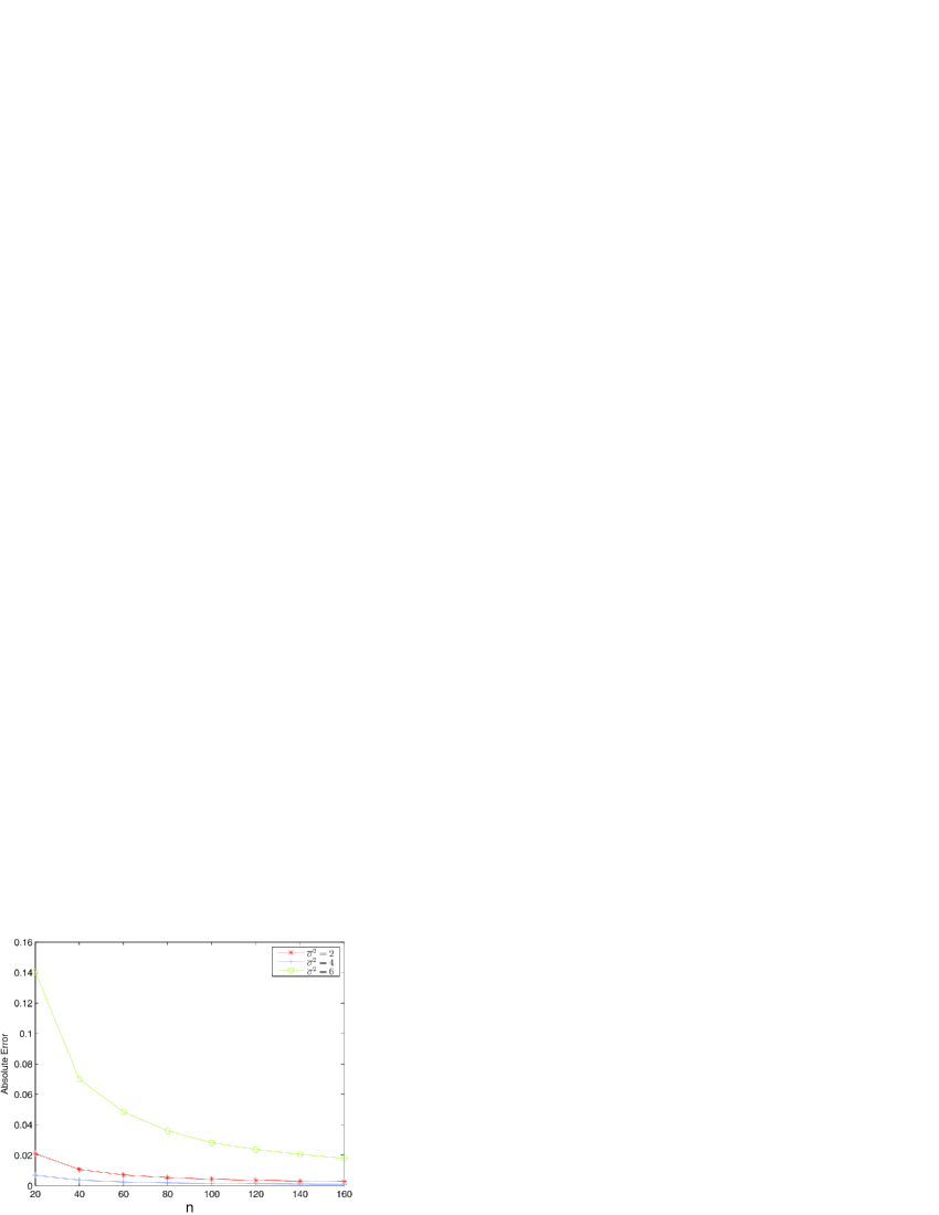
	Approx. $\bolds{n}$ $\bolds{\bar{\sigma}{}^{2}=2}$ 20 $-0.72984$ 40 $-0.74028$ 60 $-0.74382$ 80 $-0.74667$ 100 $-0.74560$ 120 $-0.74738$ 140 $-0.74790$ 160 $-0.74829$ Ans. $-0.750987$

Figure 1: A 3-dimensional example with various degrees of nonlinearity in Example 6.1.

As we can see from Figure 1, the rate of convergence is approximately $C\cdot h$, whereas the $C$ depends on the structure of $G$. Therefore, our scheme works generally for large $\Lambda$ when $\widetilde{G}$ is diagonal or diagonally dominant with a small $\theta$.

In Figure 2 we compare the convergence of our scheme with that of finite difference method by fixing $\underaccent{\bar}{\sigma}=1$, $\bar{\sigma}=\sqrt{2}$. It can be seen that our result converges slightly slower than, but is comparable to, the finite difference method in solving low-dimensional problems.

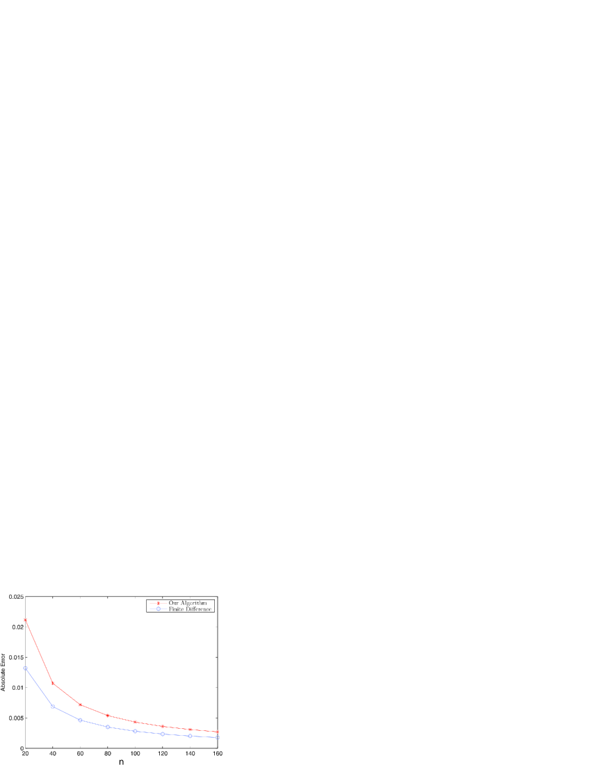
	$\bolds{n}$ Ours F.D. 20 $-$0.72984 $-$0.76420 40 $-$0.74028 $-$0.75785 60 $-$0.74382 $-$0.75562 80 $-$0.74667 $-$0.75447 100 $-$0.74560 $-$0.75379 120 $-$0.74738 $-$0.75332 140 $-$0.74790 $-$0.75300 160 $-$0.74829 $-$0.75274 Ans. $-$0.75099 $-$0.75099

Figure 2: Comparison with finite difference method in Example 6.1.

To see more of our scheme in extreme condition, we assume $\underaccent{\bar}{\sigma}=0$. Then we truncate $G_{\gamma}$ from below with a positive definite matrix $\varepsilon I_{d}>0$. That is, we approximate (6.1) by the following nondegenerate PDE:

$$-\partial_{t}u-\frac{1}{2}\sup_{{\varepsilon}\leq\sigma\leq\bar{\sigma}}\bigl{[}\bigl{(}\sigma^{2}I_{d}\bigr{)}\dvtx D^{2}u\bigr{]}+f(t,x,u,Du)=0,\qquad\varepsilon=0.01,$$

where $f$ is given by (53) (with $\underaccent{\bar}{\sigma}=0$).

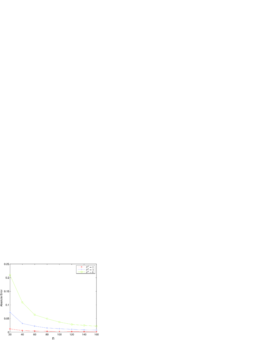
	Approx. $\bolds{n}$ $\bolds{\bar{\sigma}{}^{2}=2}$ 20 $-0.76285$ 40 $-0.75705$ 60 $-0.75508$ 80 $-0.75401$ 100 $-0.75339$ 120 $-0.75297$ 140 $-0.75269$ 160 $-0.75247$ Ans. $-0.750987$

Figure 3: Convergence of a degenerate PDE truncated in Example 6.1.

Figure 3 shows the feasibility of truncation in dealing with $\underaccent{\bar}{\sigma}=0$.

Example 6.2 ([A 4-dimensional PDE with $(\sigma_{0},p)$ depending on $(t,x)$]).

$$\cases{-\partial_{t}u-G\bigl{(}D^{2}u\bigr{)}+f(t,x)=0,&\quad in $[0,T)\times\mathbb{R}^{4}$,\vspace*{3pt}\cr u(T,x)=\operatorname{SIN}(T,x),&\quad on $\mathbb{R}^{4}$,}$$ (54)

where $\operatorname{SIN}_{2}:=2\operatorname{SIN}\times\operatorname{COS}$, and

$$\underaccent{\bar{}}{\sigma} = \pmatrix{1&0&0&0\cr\operatorname{SIN}&1&0&0\cr\operatorname{COS}&\operatorname{SIN}&1&0\cr\operatorname{SIN}&\operatorname{COS}&\operatorname{SIN}&1},\qquad A=\pmatrix{1&\displaystyle{2\operatorname{SIN}\over 27}&\displaystyle{\operatorname{SIN}_{2}\over 54}&\displaystyle{\operatorname{SIN}_{2}\over 54}\vspace*{5pt}\cr\displaystyle{2\operatorname{SIN}\over 27}&1&\displaystyle{2\operatorname{SIN}\over 27}&\displaystyle{\operatorname{SIN}_{2}\over 54}\vspace*{5pt}\cr\displaystyle{\operatorname{SIN}_{2}\over 54}&\displaystyle{2\operatorname{SIN}\over 27}&1&\displaystyle{2\operatorname{SIN}\over 27}\vspace*{5pt}\cr\displaystyle{\operatorname{SIN}_{2}\over 54}&\displaystyle{\operatorname{SIN}_{2}\over 54}&\displaystyle{2\operatorname{SIN}\over 27}&1};$$

$$\Gamma = {4\over 5}\cdot{(6-|\operatorname{SIN}|)(3-2|\operatorname{SIN}|)\over(3-|\operatorname{SIN}|)^{2}}={4\over 5}\biggl{(}2-{2|\operatorname{SIN}|\over(3-|\operatorname{SIN}|)^{2}}\biggr{)}\in\biggl{[}1,{8\over 5}\biggr{]};$$

$$\underaccent{\bar}{a} := \underaccent{\bar}{\sigma}\underaccent{\bar}{\sigma}{}^{T},\qquad\bar{a}=\Gamma\bigl{[}\underaccent{\bar}{\sigma}A\underaccent{\bar}{\sigma}{}^{T}\bigr{]},\qquad G(M):=\max\{\underaccent{\bar}{a}\dvtx M,\bar{a}\dvtx M\};$$

and $f$ is chosen so that $u:=\operatorname{SIN}$ is a classical solution of the PDE.

We first specify the parameters so that monotonicity Assumption 3.4 holds. Set $\sigma_{0}:=\beta\underaccent{\bar}{\sigma}$ for some scalar function $\beta>0$. Then, roughly speaking, $\widetilde{G}_{\gamma}$ is either ${1\over\beta^{2}}I_{d}$ or ${\Gamma\over\beta^{2}}A$. This implies $D[\widetilde{G}_{\gamma}]\leq(1+\theta)\widetilde{G}_{\gamma}$ for

$$\theta:={2|\operatorname{SIN}|\over 9-2|\operatorname{SIN}|}\leq{2\over 7}={2\over d+3}.$$

Next, notice that $\Lambda:=\bar{\alpha}/\underaccent{\bar}{\alpha}=\Gamma={4\over 5}\cdot{(6-|\operatorname{SIN}|)(3-2|\operatorname{SIN}|)\over(3-|\operatorname{SIN}|)^{2}}$ and recall 3.8(ii). Set $p:={2-\theta\over 6(1+\theta)}\in[{\theta\over 2(1+\theta)},{1\over 3}]\cap(0,{1\over 3}]$. One can check that

$$\biggl{[}1+{1\over(d-1)p}\biggr{]}\biggl{[}1-{\theta\over 2(1+\theta)p}\biggr{]}>\Lambda.$$

We remark that here we do not use $p:={2\theta\over 2-(d-3)\theta}$ as specified in Remark 3.8(ii) because it becomes zero when $\theta=0$. Finally, $\beta$ is determined by

$$\beta^{2} = {1\over\underaccent{\bar}{\alpha}}=c_{p}^{2}=2p\Lambda+\alpha_{p}-2p$$

$$= {1944-24|\operatorname{SIN}|^{2}-1260|\operatorname{SIN}|\over 270(3-|\operatorname{SIN}|)}\in\biggl{[}{11\over 9},{12\over 5}\biggr{]}.$$

In particular, we emphasize that here $\sigma_{0}$ and $p$ depend on $(t,x)$.

As explained in Section 5.1, in this case we cannot use the weighted averages as in previous example. We thus use the combination of least square regression and Monte Carlo simulation. To illustrate the important role of the basis functions, we implement our scheme using three different set of basis functions:

• the true solution and its derivatives;

• second order polynomials consisting of $\{1,\{x_{i}\}_{i=1}^{d}$, $\{x_{i}x_{j}\}_{1\leq i\leq j\leq d}\}$;

• the local basis functions proposed by Bouchard and Warin BouWarin .

The idea of local basis functions is as follows. Divide the samples at each time step into $3^{d}$ local hypercubes, such that there are 3 partitions in each dimension, and there are approximately the same amount of particles in each hypercubes. Then we project samples in each hypercubes into a linear polynomial of $d+1$ degrees of freedom, so there are $3^{d}\cdot(1+d)$ local basis functions in total. Since each linear polynomial has local hypercube support, the corresponding matrix in the regression is sparse, making it easier to solve than a regression problem of dense matrix.

Set $T=0.1$, $x_{0}=(2,3,4,5)$, and thus the true solution is $\sin(2+3+4+5)\approx 0.9906$. As our first example using Monte Carlo regression, we will sample $L=3125n^{2}$ to see how the convergence works. Moreover, we shall repeat the tests identically and independently for $K$ times. The numerical results are reported in Figure 4, where the average of the results is denoted as Ans. and the average time (in seconds) is denoted as Cost.

Basis functions			Polynomials		Local basis		True solution basis
$\bolds{n}$	$\bolds{L}$	$\bolds{K}$	Ans.	Cost	Ans.	Cost	Ans.	Cost
3	$28{,}125$	$27$	$1.094$	0.27	1.1057	0.47	$1.0959$	0.17
5	$78{,}125$	$16$	$1.0488$	1.6	1.0679	2.8	$1.0421$	0.89
10	$312{,}500$	$8$	$1.0271$	16	1.0390	34	$1.0123$	8.6
15	$703{,}125$	$6$	$1.0261$	58	1.0311	142	$1.0008$	30
20	$1{,}250{,}000$	$4$	$1.0221$	137	1.0258	355	$1.001$	71
25	$1{,}953{,}125$	$4$	$1.0240$	276	1.0247	710	$0.9986$	142
30	$2{,}812{,}500$	$3$	$1.0228$	444	1.0209	1250	$0.9966$	243
40	$5{,}000{,}000$	$2$	$1.0218$	897	1.0156	2725	$0.9952$	567
True solution			0.9906		0.9906		0.9906

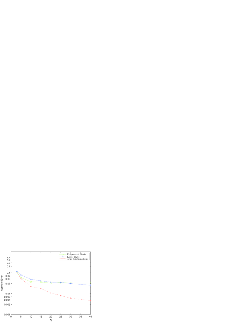
Figure 4: Numerical results using different basis functions in Example 6.2.

Without surprise, the true solution basis functions perform the best. We remark that the results for the other two sets of basis functions include the regression error as well. From the numerical results, the local basis functions seem to have smaller regression error than the polynomials, when $n$ is large. However, when applying the local basis functions it is time consuming to sort the $L$ sample paths and localize them into different hypercubes. When the same number of paths are sampled, the more basis functions we used, the slower simulation will be. More seriously, when the dimension $d$ increases, the number of basis functions increases dramatically, which requires an exponential increase in the number of paths in return; see Glasserman for a detailed investigation of the relation between basis functions and paths. So further efforts are needed for higher-dimensional problems.

Our main motivation is to provide an efficient algorithm for high-dimensional PDEs. At below we test our scheme on a 12-dimensional example, for which we shall again use the regression-based Monte Carlo method.

Example 6.3 ((A 12-dimensional example)).

Consider the PDE (6.1) with $d=12$, $\underaccent{\bar}{\sigma}=1$, $\bar{\sigma}=\sqrt{2}$,

$$f(t,x,y,z)=\operatorname{COS}-\frac{d}{2}\inf_{\underaccent{\bar}{\sigma}\leq\sigma\leq\bar{\sigma}}\bigl{(}\sigma^{2}\operatorname{SIN}\bigr{)}.$$ (55)

The true solution is again $u=\operatorname{SIN}$. As explained in Section 5.4, in this paper we want to focus on the discretization error and simulation error, so we rule out the regression error and test our algorithm by using the following perfect set of basis functions:

$$1,\qquad x,\qquad\operatorname{SIN}(T,x),\qquad\operatorname{COS}(T,x).$$

To test the result, we fix $T=0.2$ and $x_{0}=\{1,2,\ldots,12\}$, which implies that the true solution is $\sin(78)=0.513978$. As the nonlinear term is diagonal, under the same framework as in Example 6.1, we take $p:=\min\{1/3,1/(1+d(\Lambda-1))\}=1/13$, $\sigma_{0}:=I_{d}$, which also satisfy the monotonicity condition Assumption 3.4. Assuming that we repeat $K$ identical and independent tests, and we sample $L$ paths in each test. We do not use $L=O(N^{3})$ in this example and the ones following, since it’s usually not necessary in practice. The results are reported in Figure 5, where we conduct fewer tests for larger $L$, because the results are stable enough to draw our conclusion.

$\bolds{n}$	$\bolds{L}$	$\bolds{K}$	Avg(Ans.)	Var(Avg.)	Cost (in seconds)
2	$2083$	$160$	0.659639	$3.53\times 10^{-6}$	$4.48\times 10^{-2}$
5	$13{,}021$	$64$	0.562635	$1.99\times 10^{-6}$	$1.46\times 10^{-1}$
10	$52{,}083$	$32$	0.546598	$8.41\times 10^{-7}$	$1.17\times 10^{0}$
20	$208{,}333$	$16$	0.530432	$8.04\times 10^{-7}$	$1.08\times 10^{1}$
40	$833{,}333$	$8$	0.521343	$2.25\times 10^{-7}$	$9.11\times 10^{1}$
80	$3{,}333{,}333$	$4$	0.519701	$1.21\times 10^{-7}$	$7.28\times 10^{2}$
160	$13{,}333{,}333$	$2$	0.517363	$6.17\times 10^{-8}$	$5.86\times 10^{3}$
True solution			0.513978

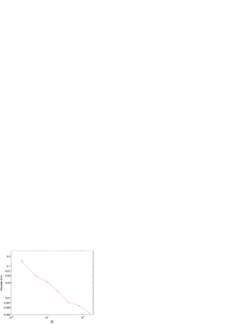
Figure 5: Numerical results of a 12-dimensional example in Example 6.3.

It can be seen from Figure 5 that the error shrinks slightly slower than $O(h)$, which is due to the simulation error. Hence we want to explore the influence of simulation error by using all the parameters as above but fixing $n=40$, $K=2$, $d=12$, $T=0.2$, $n=40$, $\underaccent{\bar}{\sigma}=1$, $\bar{\sigma}=\sqrt{2}$. We increase the sample size $L$ to see how the error reduces in Figure 6. While the variance and error decrease with more paths sampled, the cost in time increases linearly with respect to $L$ from 8 seconds to 1400 seconds in Figure 6.

	$\bolds{L}$ Approx.   000,83,333 0.543643   00,166,667 0.526979   00,416,667 0.523897   00,833,333 0.524683 1,666,667 0.521531   00,333,333 0.521017 6,666,667 0.520083 13,333,333 0.518607 Ans.: 0.513978

Figure 6: Relation between size of sample and errors in Example 6.3.

We have seen that our scheme converges to the true classical solution if it exists. Meanwhile, if the PDE only has a unique viscosity solution, our scheme can render a converging result as well.

Let $f$ be zero in (6.1). Then this equation has some unknown viscosity solution. However, our numerical results in Figure 7 still demonstrate a converging sequence. The number of paths we sampled in 7 is the same as that in Figure 5. This can be also be observed from the decreasing differences between the numerical results. The $\Delta_{i-j}$ in Figure 7 denotes a numerical result with $i$ partitions in time minus another numerical result with $j$ time steps. We shall remark though in this case our choice of basis functions may not be the best, and roughly speaking the numerical result we obtain is an approximation of the regression of the true solution in the linear span of the basis functions. Again, we leave the analysis of the basis functions to future study.

	$\Delta_{5-2}$ 0.0334337 $\Delta_{10-5}$ 0.0077685 $\Delta_{20-10}$ 0.0076637 $\Delta_{40-20}$ 0.0034146 $\Delta_{80-40}$ 0.0012785 $\Delta_{160-80}$ 0.0002586

Figure 7: Numerical results for a PDE with unknown viscosity solution in Example 6.3.

It is well known that Isaacs equations have a unique viscosity solution under mild technical conditions. We next test our scheme on the following Isaacs equation to see its performance.

Example 6.4 ((A 12-dimensional Isaacs equation with unknown viscosity solution)).

$$-u_{t}-G\bigl{(}D^{2}u\bigr{)} = 0\qquad\mbox{on }[0,T)\times\mathbb{R}^{d},$$

$$u(T,x) = \operatorname{SIN}(T,x)\qquad\mbox{on }\mathbb{R}^{d},$$

where

$$G(\gamma) := \sum_{i=1}^{d}\sup_{0\leq u\leq 1}\inf_{{0\leq v\leq 1}}\biggl{[}\frac{1}{2}\sigma^{2}(u,v)\gamma_{ii}+f(u,v)\biggr{]}$$

$$= \sum_{i=1}^{d}\inf_{{0\leq v\leq 1}}\sup_{0\leq u\leq 1}\biggl{[}\frac{1}{2}\sigma^{2}(u,v)\gamma_{ii}+f(u,v)\biggr{]},$$

$$\sigma^{2}(u,v) := (1+u+v),\qquad f(u,v):=-\frac{u^{2}}{4}+\frac{v^{2}}{4}.$$

One can easily simplify $G(\gamma)$ as: $G(\gamma)=\sum_{i=1}^{d}g(\gamma_{ii})$ where

$$g(\gamma_{ii}) := \cases{\displaystyle\gamma_{ii}-\frac{1}{4},&\quad$\gamma_{ii}\in(1,+\infty)$,\vspace*{5pt}\cr\displaystyle\frac{\gamma_{ii}}{2}+\frac{(\gamma_{ii}^{+})^{2}}{4}-\frac{(\gamma_{ii}^{-})^{2}}{4},&\quad$\gamma_{ii}\in[-1,1]$,\vspace*{5pt}\cr\displaystyle\gamma_{ii}+\frac{1}{4},&\quad$\gamma_{ii}\in(-\infty,-1)$.}$$

Therefore $G(\gamma)$ is neither concave nor convex when $\gamma=0$. Setting $T=0.2$, $d=12$, we assign arbitrary initial value $x_{0}=\{x_{0}^{(i)}\}_{i=1}^{d}$ to inspect the outcome. Obviously here $\bar{a}=2I_{d}$ and $\underaccent{\bar}{a}=I_{d}$. We then take $p=\min\{1/3,1/(1+d(\Lambda-1))\}=1/13$, $\sigma_{0}=I_{d}$. One example tested here is $x_{0}^{(i)}=2i\pi-\frac{T-0.5\pi}{d}$. The number of paths we sampled is $625\cdot n^{2}$.

Though the viscosity solution is unknown, our scheme still renders a converging numerical result in Figure 8.

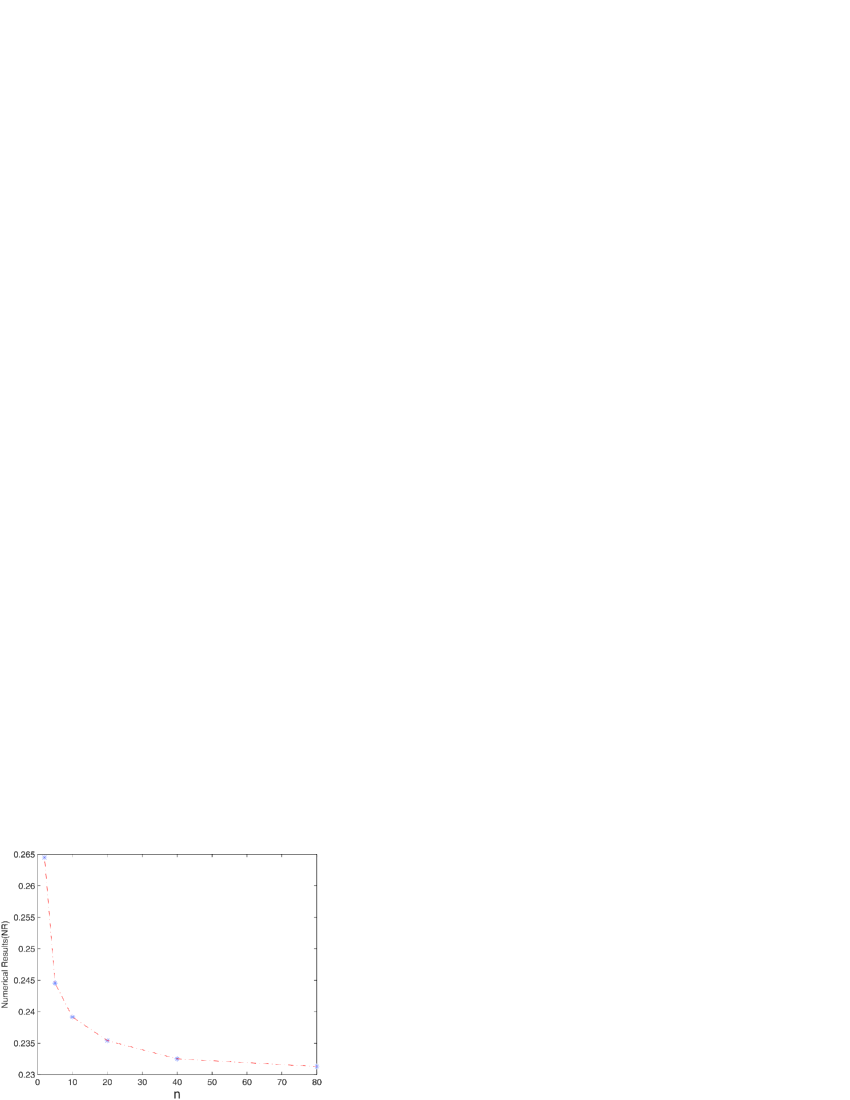
	$\Delta_{5-2}$ $-$0.019953 $\Delta_{10-5}$ $-$0.005390 $\Delta_{20-10}$ $-$0.003752 $\Delta_{40-20}$ $-$0.002893 $\Delta_{80-40}$ $-$0.001213 $\Delta_{160-80}$ $-$0.000426

Figure 8: A 12-dimensional Isaacs equation with unknown viscosity solution in Example 6.4.

We next test our scheme for a $12$-dimensional coupled FBSDE.

Example 6.5 ((A 12-dimensional coupled FBSDE)).

Consider FBSDE (38) with $m=d=12$, $\sigma$ is diagonal, and

$$b_{i}(t,x,y,z) := \cos(y+z_{i}),\qquad\sigma_{ii}(t,x,y):=1+\frac{1}{3}\sin\Biggl{(}\frac{1}{d}\sum_{j=1}^{d}x_{j}+y\Biggr{)},$$

$$f(t,x,y,z) := \frac{d}{2}\operatorname{SIN}(t,x)\Biggl{[}1+\frac{1}{3}\sin\Biggl{(}\frac{1}{d}\sum_{i=1}^{d}x_{i}+y\Biggr{)}\Biggr{]}^{2}$$

$${}-\frac{{(1/d)}\sum_{i=1}^{d}z_{i}}{1+({1}/{3})\sin(({1}/{d})\sum_{j=1}^{d}x_{j}+y)}$$

$${}-d\operatorname{COS}(t,x)\cos\bigl{(}y+\operatorname{COS}(t,x)\bigr{)};$$

$$g(x) := \operatorname{SIN}(T,x).$$

The associated PDE (4) looks quite complicated; however, the coefficients are constructed in a way so that $u:=\operatorname{SIN}$ is the classical solution. Consequently, the FBSDE has the following solution: denoting $\overline{X}_{t}:={1\over d}\sum_{j=1}^{d}X^{j}_{t}$,

$$Y_{t}=\sin(t+d\overline{X}_{t}),\qquad Z^{i}_{t}=\cos(t+d\overline{X}_{t})\bigl{[}1+\tfrac{1}{3}\sin\bigl{(}\overline{X}_{t}+\sin(t+d\overline{X}_{t})\bigr{)}\bigr{]}.$$

For PDE (4), we see that $G_{\gamma}=\frac{1}{2}\sigma^{2}$ is diagonal and ${2\over 3}\leq\sigma_{ii}\leq{4\over 3}$ for each $i$. Hence a reasonable choice of parameters that maintains the monotonicity would be $\sigma_{0}:={4\over 9}I_{d}$, $p:=\min\{{1\over 1+d(\Lambda-1)}$, ${1\over 3}\}=1/37$. We note that $f$ is not bounded and not Lipschitz continuous in $y$; however, since $Z$ is bounded, then $f(t,x,y,Z_{t})$ is bounded and Lipschitz continuous in $y$, and thus actually we may still apply Theorem 4.1. Set $d=12$, $T=0.2$, $X_{0}=(2,3,4,\ldots,13)$, and apply the parameters specified before for our scheme. An approximation of $Y_{0}$ is shown in Figure 9, where the true solution $Y_{t}=\sin(t+\sum_{i=1}^{d}X_{t}^{i})$ has value 0.893997 at $t=0$.

$\bolds{n}$	$\bolds{L}$	$\bolds{K}$	Avg(Ans.)	Var(Avg.)	Cost (in seconds)
2	$2083$	$160$	1.462543	$3.35\times 10^{-5}$	$1.56\times 10^{-2}$
5	$13{,}021$	$64$	1.111675	$2.30\times 10^{-5}$	$2.36\times 10^{-1}$
10	$52{,}083$	$32$	1.014295	$2.48\times 10^{-5}$	$2.43\times 10^{0}$
20	$20{,}8333$	$16$	0.925712	$8.10\times 10^{-6}$	$2.29\times 10^{1}$
40	$83{,}3333$	$8$	0.912373	$2.46\times 10^{-6}$	$1.94\times 10^{2}$
80	$3{,}333{,}333$	$4$	0.908013	$2.89\times 10^{-7}$	$1.56\times 10^{3}$
160	$13{,}333{,}333$	$2$	0.888747	$1.62\times 10^{-8}$	$3.42\times 10^{4}$

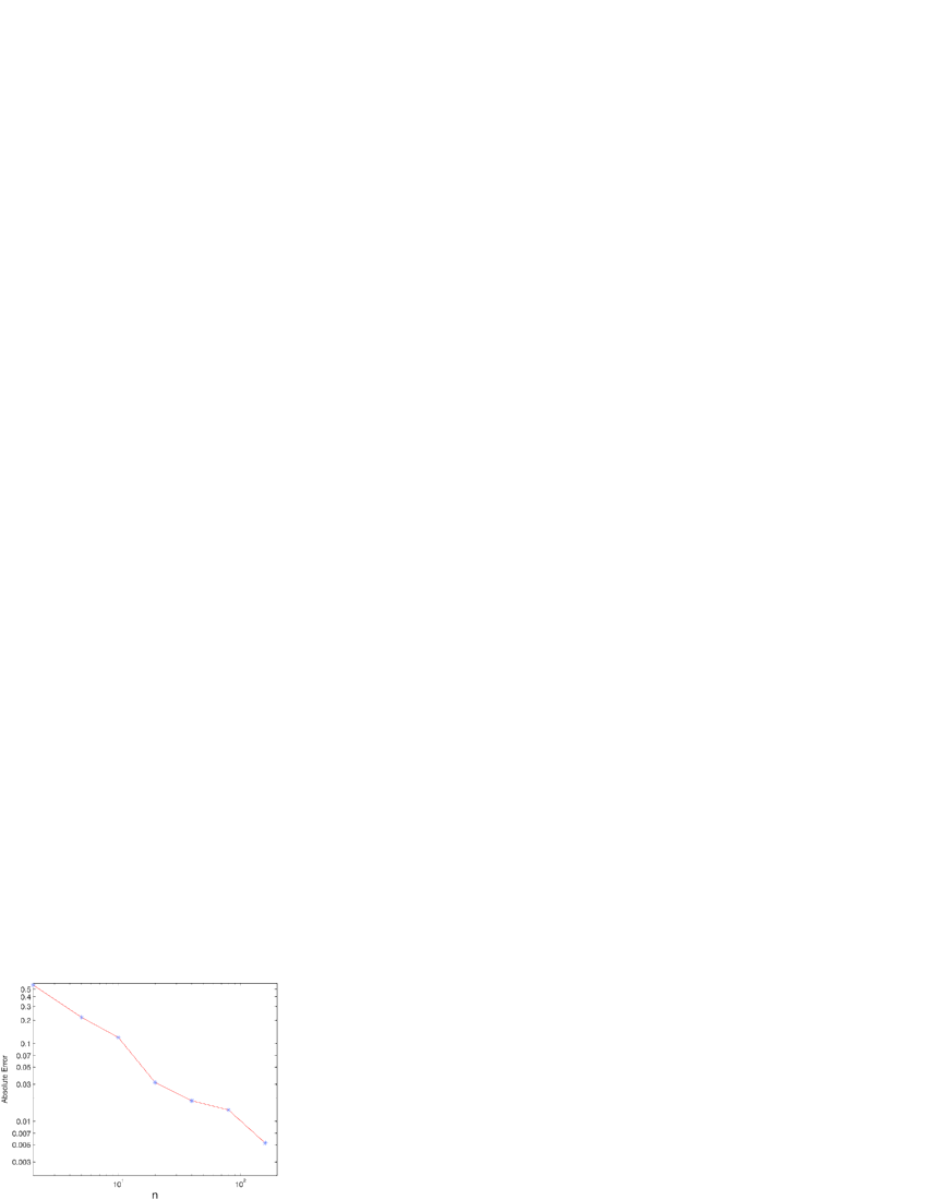
Figure 9: A 12-dimensional coupled FBSDE in Example 6.5.

6.2 Examples violating the monotonicity condition

In this subsection we apply our scheme to some examples which do not satisfy our monotonicity Assumption 3.4. So theoretically we do not know if our scheme converges or not. However, our numerical results show that the approximation still converges to the true solution. It will be very interesting to understand the scheme under these situations, and we shall leave it for future research.

Example 6.6 ((A 12-dimensional PDE with $\underaccent{\bar}{\sigma}=0$)).

Consider the same setting as Example 6.3 except that $\underaccent{\bar}{\sigma}=0$.

Instead of truncating $G_{\gamma}$ as we did at the end of Example 6.1, we will pick parameters $p$ and $\sigma_{0}$ as if $\underaccent{\bar}{\sigma}$ were some small positive number: $p:=1/d$, $\sigma_{0}:=\sqrt{2/(2-p)}\bar{\sigma}I_{d}$. Then Assumption 3.4 is violated, and our scheme is in fact not monotone. Nevertheless, our numerical results show that our approximations still converge to the true solution if $L:=625n^{2}$ paths are used; see Figure 10.

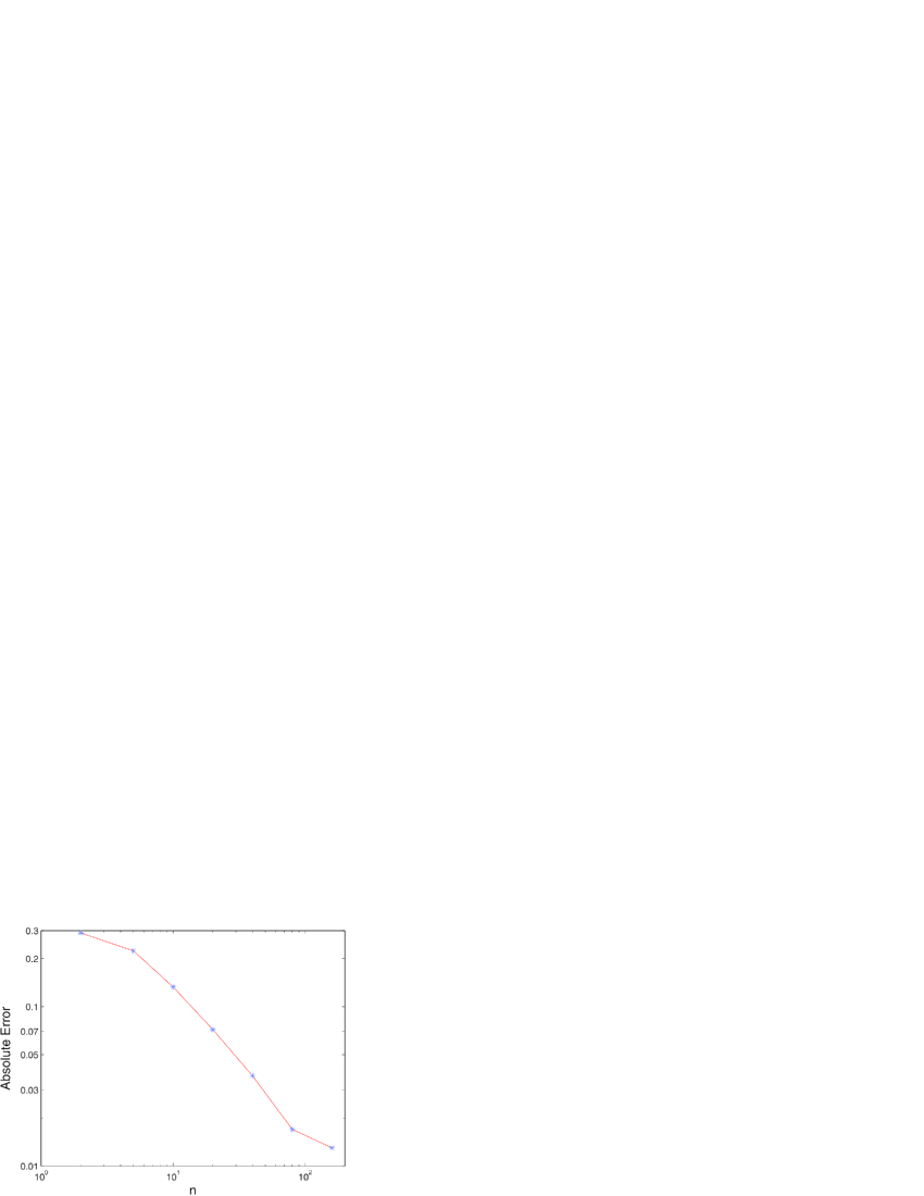
	$\bolds{n}$ Approx. 2 0.22363 5 0.28971 10 0.38098 20 0.44215 40 0.47712 80 0.49699 160 0.50097 Ans. 0.51398

Figure 10: A 12-dimensional example without monotonicity in Example 6.6.

We next apply our scheme to the following HJB equation which is associated with a Markovian second order BSDEs, introduced by CSTV , STZ :

$$\qquad\cases{\displaystyle-\frac{\partial u}{\partial t}-\frac{1}{2}\sup_{\underaccent{\bar}{\sigma}\leq\sigma\leq\bar{\sigma}}\bigl{[}\sigma^{2}\dvtx D^{2}u\bigr{]}-f(t,x)=0,&\quad on $[0,T)\times\mathbb{R}^{d}$,\vspace*{5pt}\cr u(T,x)=g(x),&\quad on $\mathbb{R}^{d}$.}$$ (56)

When $f=0$, this PDE induces exactly the $G$-expectation introduced by Peng Peng . We emphasize that, unlike in previous examples, here $\underaccent{\bar}{\sigma},\bar{\sigma},\sigma\in\mathbb{S}^{d}$ are matrices and ${\mathbf{0}}<\underaccent{\bar}{\sigma}\leq\sigma\leq\bar{\sigma}$. In particular, $G_{\gamma}$ is not diagonal anymore. We remark that one has a representation for the solution of this PDE in terms of stochastic control,

$$u(0,x) = \sup_{\sigma}\mathbb{E}\biggl{[}g\bigl{(}X^{\sigma}_{T}\bigr{)}+\int_{0}^{T}f\bigl{(}t,X^{\sigma}_{t}\bigr{)}\,dt\biggr{]},\qquad X^{\sigma}_{t}:=x+\int_{0}^{t}\sigma_{s}\,dW_{s},$$

where $W$ is a $d$-dimensional Brownian motion, and the control $\sigma$ is an $\mathbb{F}^{W}$-progressively measurable $\mathbb{S}^{d}$-valued process such that $\underaccent{\bar}{\sigma}\leq\sigma\leq\bar{\sigma}$. Due to this connection, these kind of PDEs and the related $G$-expectation and second order BSDEs are important in applications with diffusion control and/or volatility uncertainty.

Example 6.7 ((A 10-dimensional HJB equation)).

Consider the PDE (56) with $g(x)=\sin(T+x_{1}+{x_{2}\over 2}+\cdots+{x_{d}\over d})$ and appropriate $f(t,x)$ so that

$$u(t,x) = \sin\biggl{(}t+x_{1}+{x_{2}\over 2}+\cdots+{x_{d}\over d}\biggr{)}$$

is the true solution to the PDE. We set $d=10$.

To begin our test, we select randomly an initial point $X_{0}$ and two 10-dimensional positive definite matrices $\bar{\sigma}{}^{2}$ and $\underaccent{\bar}{\sigma}{}^{2}$. The parameters used in this PDE are chosen randomly as:

$$X_{0} = (0.8870626082,1.8313582937,2.1710945122,2.3703744353,$$

$$\hskip 3.0pt1.2018847713,2.6518851292,2.2648022663,1.9037585152,$$

$$\hskip 117.0pt2.336892572579084,1.1590768112),$$

which gives a true solution $-$0.99966,

$$\bar{\sigma}{}^{2}=\\ \pmatrix{2.29&0.07&-0.48&0.15&0.89&-0.06&0.14&0.31&0.59&-0.36\vspace*{3pt}\cr 0.07&1.82&0.55&0.32&0.28&0.08&-0.30&-0.07&-0.46&0.66\vspace*{3pt}\cr-0.48&0.55&2.54&-0.35&0.14&-0.25&-0.31&0.16&-0.71&-0.10\vspace*{3pt}\cr 0.15&0.32&-0.35&1.71&-0.16&0.67&0.20&1.11&-0.03&-0.64\vspace*{3pt}\cr 0.89&0.28&0.14&-0.16&1.36&-0.47&-0.46&0.07&-0.07&-0.03\vspace*{3pt}\cr-0.06&0.08&-0.25&0.67&-0.47&2.60&0.26&0.34&-0.02&-0.67\vspace*{3pt}\cr 0.14&-0.30&-0.31&0.20&-0.46&0.26&2.61&-0.26&0.32&0.29\vspace*{3pt}\cr 0.31&-0.07&0.16&1.11&0.07&0.34&-0.26&2.66&-0.19&-1.78\vspace*{3pt}\cr 0.59&-0.46&-0.71&-0.03&-0.07&-0.02&0.32&-0.19&1.80&-0.43\vspace*{3pt}\cr-0.36&0.66&-0.10&-0.64&-0.03&-0.67&0.29&-1.78&-0.43&2.16}$$

and

$$\underaccent{\bar}{\sigma}{}^{2}=\pmatrix{1.53&-0.40&-0.30&-0.20&0.66&-0.43&0.38&0.10&0.84&-0.31\vspace*{3pt}\cr-0.40&0.72&0.58&-0.06&-0.15&-0.28&-0.07&-0.14&-0.32&0.42\vspace*{3pt}\cr-0.30&0.58&1.55&-0.05&-0.07&-0.54&-0.03&-0.20&-0.51&0.38\vspace*{3pt}\cr-0.20&-0.06&-0.05&0.55&-0.14&0.22&-0.09&0.60&-0.13&-0.37\vspace*{3pt}\cr 0.66&-0.15&-0.07&-0.14&0.61&-0.50&-0.09&-0.10&0.25&-0.12\vspace*{3pt}\cr-0.43&-0.28&-0.54&0.22&-0.50&1.27&0.15&0.34&-0.06&-0.21\vspace*{3pt}\cr 0.38&-0.07&-0.03&-0.09&-0.09&0.15&1.78&0.13&-0.24&0.17\vspace*{3pt}\cr 0.10&-0.14&-0.20&0.60&-0.10&0.34&0.13&1.04&0.16&-0.94\vspace*{3pt}\cr 0.84&-0.32&-0.51&-0.13&0.25&-0.06&-0.24&0.16&1.22&-0.56\vspace*{3pt}\cr-0.31&0.42&0.38&-0.37&-0.12&-0.21&0.17&-0.94&-0.56&1.36}.$$

One can check that $\bar{\sigma}{}^{2}>\underaccent{\bar}{\sigma}{}^{2}$ because the smallest eigenvalue of $\bar{\sigma}{}^{2}-\underaccent{\bar}{\sigma}{}^{2}$ is $0.001634$, which is positive. This PDE is not diagonally dominant, and typically we cannot find $\sigma_{0}$ and $p$ to make our scheme monotone. However, it is very interesting to observe that our scheme converges to the true solution if we choose $p:=1/3$ and $\sigma_{0}:={d\sqrt{d}\over 2\sqrt{d+1}}\sqrt{\bar{\sigma}{}^{2}}$; see Figure 11. We emphasize again that these parameters still do not satisfy Assumption 3.4. It will be very interesting to understand further these numerical results, and we will leave them for future research.

$\bolds{n}$	$\bolds{L}$	$\bolds{K}$	Avg(Ans.)	Var(Avg.)	Cost (in seconds)
2	$283$	$40$	$-1.1703$	$9.62\times 10^{-7}$	0.057
5	$1118$	$16$	$-1.12773$	$3.80\times 10^{-6}$	1.9
10	$3162$	$8$	$-1.0802$	$5.98\times 10^{-6}$	$23.6$
15	$5809$	$5$	$-1.0557$	$2.32\times 10^{-6}$	$103$
20	$8944$	$4$	$-1.0405$	$1.57\times 10^{-6}$	$291$
30	$16{,}432$	$3$	$-1.0253$	$9.05\times 10^{-6}$	$1135$
40	$25{,}298$	$2$	$-1.0124$	$2.16\times 10^{-5}$	$3074$
True solution			$-0.99966$

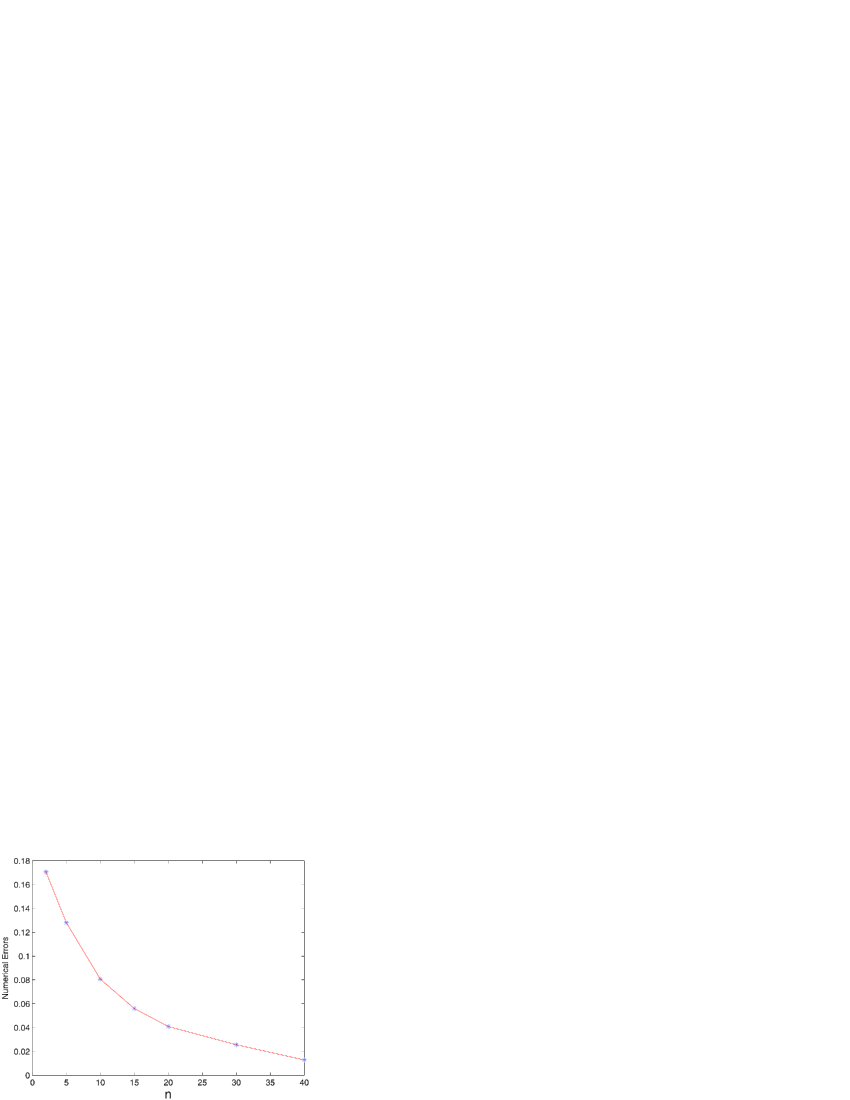
Figure 11: A 10-dimensional HJB equation in Example 6.7.

Note that PDE (56) involves the computation of $\sup_{\underaccent{\bar}{\sigma}\leq\sigma\leq\bar{\sigma}}[\sigma^{2}\dvtx\gamma]$. We provide some discussion below.

Remark 6.8.

Let $\bar{\sigma}{}^{2}-\underaccent{\bar}{\sigma}{}^{2}=LL^{T}$ be the Cholesky Decomposition, namely $L$ is a $d\times d$ lower triangular matrix. Then for any $\gamma\in\mathbb{S}^{d}$, we have

$$\sup_{\underaccent{\bar}{\sigma}{}^{2}\leq\sigma^{2}\leq\bar{\sigma}{}^{2}}\bigl{[}\sigma^{2}\dvtx\gamma\bigr{]}=\underaccent{\bar}{\sigma}{}^{2}\dvtx\gamma+\sum_{i=1}^{n}\hat{\gamma}_{i}^{+},$$

where $\hat{\gamma}_{i}$, $i=1,\ldots,d$, are the eigenvalues of $L^{T}\gamma L$.

Obviously, any $\sigma^{2}\in\mathbb{S}^{d}$ between $\underaccent{\bar}{\sigma}{}^{2}$ and $\bar{\sigma}{}^{2}$ can be expressed as $\sigma^{2}=\underaccent{\bar}{\sigma}{}^{2}+A$, where ${\mathbf{0}}\leq A\leq LL^{T}$. Then ${\mathbf{0}}\leq L^{-1}AL^{-T}\leq I_{d}$. We make the following eigenvalue decompositions:

$$L^{-1}AL^{-T}=U\widehat{A}U^{T},\qquad L^{T}\gamma L=P\hat{\gamma}P^{T},$$

where $UU^{T}=PP^{T}=I_{d}$, and $\widehat{A}$ and $\hat{g}$ diagonal matrices. It is clear that the diagonal terms of $\widehat{A}$ are $\hat{a}_{i}\in[0,1]$, and the diagonal terms of $\hat{\gamma}$ are $\hat{\gamma}_{i}$. Denote $Q:=U^{T}P$. Then

$$\sigma^{2}\dvtx\gamma-\underaccent{\bar}{\sigma}{}^{2}\dvtx\gamma = A\dvtx\gamma=\bigl{[}L^{-1}AL^{-T}\bigr{]}\dvtx\bigl{[}L^{T}\gamma L\bigr{]}=\bigl{[}U\widehat{A}U^{T}\bigr{]}\dvtx\bigl{[}L^{T}\gamma L\bigr{]}$$

$$= \widehat{A}\dvtx\bigl{[}U^{T}L^{T}\gamma LU\bigr{]}=\widehat{A}\dvtx\bigl{[}Q\hat{\gamma}Q^{T}\bigr{]}$$

$$= \sum_{i=1}^{d}\hat{a}_{i}\sum_{j=1}^{d}q_{ij}^{2}\hat{\gamma}_{j}\leq\sum_{i=1}^{d}\Biggl{(}\sum_{j=1}^{d}q_{ij}^{2}\hat{\gamma}_{j}\Biggr{)}^{+}.$$

Note that $\sum_{j=1}^{d}q_{ij}^{2}=1$. Then by Jensen’s inequality,

$$\sigma^{2}\dvtx\gamma-\underaccent{\bar}{\sigma}{}^{2}\dvtx\gamma\leq\sum_{i=1}^{d}\Biggl{(}\sum_{j=1}^{d}q_{ij}^{2}\hat{\gamma}_{j}\Biggr{)}^{+}\leq\sum_{i=1}^{d}\sum_{j=1}^{d}q_{ij}^{2}\hat{\gamma}_{j}^{+}=\sum_{j=1}^{d}\hat{\gamma}_{j}^{+}\sum_{i=1}^{d}q_{ij}^{2}=\sum_{j=1}^{d}\hat{\gamma}_{j}^{+}.$$

This proves the remark.

Moreover, from the proof we see that the equality holds when

$$\hat{a}_{i}=1_{\{\sum_{j=1}^{d}q_{ij}^{2}\hat{\gamma}_{j}>0\}}\quad\mbox{and}\quad Q=I_{d}.$$

That is, $U=P$ and thus $\sigma^{2}=\underaccent{\bar}{\sigma}^{2}+LP\widehat{A}P^{T}L^{T}$, where $\widehat{A}$ is the diagonal matrix whose diagonal terms are $\hat{a}_{i}=1_{\{\hat{\gamma}_{i}>0\}}$.

We remark that the above computation is in fact quite time consuming. Below we provide another example where $G_{\gamma}$ is tridiagonal, and the scheme becomes much more efficient.

Example 6.9 ((A 10-dimensional example with tridiagonal structure)).

Consider the PDE (1) with

$$G(t,x,y,z,\gamma) := \Biggl{(}3\sum_{i=1}^{d}\gamma_{ii}+\sum_{|i-j|=1}\frac{1}{\sqrt{1+(\gamma_{ij})^{2}}}\Biggr{)}+f(t,x),$$

$$g(x) := \operatorname{SIN}(T,x),$$

and $f$ is chosen so that $u:=\operatorname{SIN}$ is the true solution of the PDE.

In this case one may check straightforwardly that

$$[G_{\gamma}]_{ii}=3\quad\mbox{and}\quad\bigl{[}G_{\gamma}(t,x,y,z,\gamma)\bigr{]}_{ij}=-\frac{\gamma_{ij}}{(1+\gamma_{ij}^{2})^{3/2}},\qquad|i-j|=1.$$

When $d=10$, this example is out of the scope of our monotonicity Assumption 3.4, even with our choice of $p$ and $\sigma_{0}$: $p:=\min({1\over 3}$, ${1\over(1+d*(5-1))})=1/41$, $\sigma_{0}=I_{d}$. However, if we test it using $T=0.2$, $x_{0}=(1,2,\ldots,10)$, the numerical results show that our scheme still converges to the true solution, $\sin(55)=-0.999755$, as presented in Figure 12.

$\bolds{n}$	$\bolds{L}$	$\bolds{K}$	Avg(Ans.)	Var(Avg.)	Cost (in seconds)
2	$2500$	$160$	$-$1.47362	$1.0\times 10^{-5}$	$1.2\times 10^{-2}$
5	$15{,}625$	$64$	$-$1.15004	$1.7\times 10^{-6}$	$1.4\times 10^{-1}$
10	$62{,}500$	$32$	$-$1.06194	$9.1\times 10^{-6}$	$1.0\times 10^{0}$
20	$250{,}000$	$16$	$-$1.04519	$2.1\times 10^{-6}$	$8.9\times 10^{0}$
40	$1{,}000{,}000$	$8$	$-$1.03326	$6.2\times 10^{-7}$	$7.1\times 10^{1}$
80	$4{,}000{,}000$	$4$	$-$1.03092	$5.8\times 10^{-8}$	$5.9\times 10^{2}$
160	$16{,}000{,}000$	$2$	$-$1.01910	$3.0\times 10^{-9}$	$1.4\times 10^{4}$

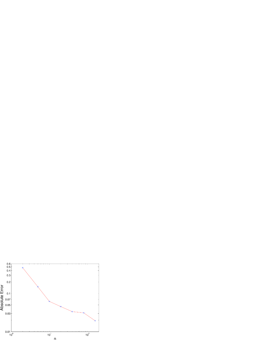
Figure 12: A 10-dimensional example with tridiagonal generator in Example 6.9.

We shall remark though that this example is computationally more expensive than Example 6.3 because here we need to approximate $3d-2$ second derivatives.

References

- (1) {barticle}[mr] \bauthor\bsnmBally, \bfnmVlad\binitsV., \bauthor\bsnmPagès, \bfnmGilles\binitsG. and \bauthor\bsnmPrintems, \bfnmJacques\binitsJ. (\byear2005). \btitleA quantization tree method for pricing and hedging multidimensional American options. \bjournalMath. Finance \bvolume15 \bpages119–168. \biddoi=10.1111/j.0960-1627.2005.00213.x, issn=0960-1627, mr=2116799 \bptokimsref\endbibitem
- (2) {barticle}[mr] \bauthor\bsnmBarles, \bfnmGuy\binitsG. and \bauthor\bsnmJakobsen, \bfnmEspen R.\binitsE. R. (\byear2007). \btitleError bounds for monotone approximation schemes for parabolic Hamilton–Jacobi–Bellman equations. \bjournalMath. Comp. \bvolume76 \bpages1861–1893 (electronic). \biddoi=10.1090/S0025-5718-07-02000-5, issn=0025-5718, mr=2336272 \bptokimsref\endbibitem
- (3) {barticle}[mr] \bauthor\bsnmBarles, \bfnmG.\binitsG. and \bauthor\bsnmSouganidis, \bfnmP. E.\binitsP. E. (\byear1991). \btitleConvergence of approximation schemes for fully nonlinear second order equations. \bjournalAsymptot. Anal. \bvolume4 \bpages271–283. \bidissn=0921-7134, mr=1115933 \bptokimsref\endbibitem
- (4) {barticle}[mr] \bauthor\bsnmBender, \bfnmChristian\binitsC. and \bauthor\bsnmDenk, \bfnmRobert\binitsR. (\byear2007). \btitleA forward scheme for backward SDEs. \bjournalStochastic Process. Appl. \bvolume117 \bpages1793–1812. \biddoi=10.1016/j.spa.2007.03.005, issn=0304-4149, mr=2437729 \bptokimsref\endbibitem
- (5) {bincollection}[auto:STB—2014/02/12—14:17:21] \bauthor\bsnmBender, \bfnmC.\binitsC. and \bauthor\bsnmSteiner, \bfnmJ.\binitsJ. (\byear2012). \btitleLeast-squares Monte Carlo for BSDEs. In \bbooktitleNumerical Methods in Finance (\beditor\bfnmR. A.\binitsR. A. \bsnmCarmona, \beditor\bfnmP.\binitsP. \bsnmDel Moral, \beditor\bfnmP.\binitsP. \bsnmHu and \beditor\bfnmN.\binitsN. \bsnmOudjane, eds.). \bseriesSpringer Proceedings in Mathematics \bvolume12 \bpages257–289. \bpublisherSpringer, \blocationHeidelberg. \bptokimsref\endbibitem
- (6) {barticle}[mr] \bauthor\bsnmBender, \bfnmChristian\binitsC. and \bauthor\bsnmZhang, \bfnmJianfeng\binitsJ. (\byear2008). \btitleTime discretization and Markovian iteration for coupled FBSDEs. \bjournalAnn. Appl. Probab. \bvolume18 \bpages143–177. \biddoi=10.1214/07-AAP448, issn=1050-5164, mr=2380895 \bptokimsref\endbibitem
- (7) {barticle}[mr] \bauthor\bsnmBonnans, \bfnmJ. Frédéric\binitsJ. F. and \bauthor\bsnmZidani, \bfnmHousnaa\binitsH. (\byear2003). \btitleConsistency of generalized finite difference schemes for the stochastic HJB equation. \bjournalSIAM J. Numer. Anal. \bvolume41 \bpages1008–1021. \biddoi=10.1137/S0036142901387336, issn=0036-1429, mr=2005192 \bptokimsref\endbibitem
- (8) {barticle}[mr] \bauthor\bsnmBouchard, \bfnmBruno\binitsB. and \bauthor\bsnmTouzi, \bfnmNizar\binitsN. (\byear2004). \btitleDiscrete-time approximation and Monte-Carlo simulation of backward stochastic differential equations. \bjournalStochastic Process. Appl. \bvolume111 \bpages175–206. \biddoi=10.1016/j.spa.2004.01.001, issn=0304-4149, mr=2056536 \bptokimsref\endbibitem
- (9) {bincollection}[auto:STB—2014/02/12—14:17:21] \bauthor\bsnmBouchard, \bfnmB.\binitsB. and \bauthor\bsnmWarin, \bfnmX.\binitsX. (\byear2012). \btitleMonte-Carlo valuation of American options: Facts and new algorithms to improve existing methods. In \bbooktitleNumerical Methods in Finance (\beditor\bfnmR. A.\binitsR. A. \bsnmCarmona, \beditor\bfnmP.\binitsP. \bsnmDel Moral, \beditor\bfnmP.\binitsP. \bsnmHu and \beditor\bfnmN.\binitsN. \bsnmOudjane, eds.). \bseriesSpringer Proceedings in Mathematics \bvolume12 \bpages215–255. \bpublisherSpringer, \blocationHeidelberg. \bptokimsref\endbibitem
- (10) {barticle}[mr] \bauthor\bsnmCheridito, \bfnmPatrick\binitsP., \bauthor\bsnmSoner, \bfnmH. Mete\binitsH. M., \bauthor\bsnmTouzi, \bfnmNizar\binitsN. and \bauthor\bsnmVictoir, \bfnmNicolas\binitsN. (\byear2007). \btitleSecond-order backward stochastic differential equations and fully nonlinear parabolic PDEs. \bjournalComm. Pure Appl. Math. \bvolume60 \bpages1081–1110. \biddoi=10.1002/cpa.20168, issn=0010-3640, mr=2319056 \bptokimsref\endbibitem
- (11) {barticle}[mr] \bauthor\bsnmClément, \bfnmEmmanuelle\binitsE., \bauthor\bsnmLamberton, \bfnmDamien\binitsD. and \bauthor\bsnmProtter, \bfnmPhilip\binitsP. (\byear2002). \btitleAn analysis of a least squares regression method for American option pricing. \bjournalFinance Stoch. \bvolume6 \bpages449–471. \biddoi=10.1007/s007800200071, issn=0949-2984, mr=1932380 \bptokimsref\endbibitem
- (12) {barticle}[mr] \bauthor\bsnmCrandall, \bfnmMichael G.\binitsM. G., \bauthor\bsnmIshii, \bfnmHitoshi\binitsH. and \bauthor\bsnmLions, \bfnmPierre-Louis\binitsP.-L. (\byear1992). \btitleUser’s guide to viscosity solutions of second order partial differential equations. \bjournalBull. Amer. Math. Soc. (N.S.) \bvolume27 \bpages1–67. \biddoi=10.1090/S0273-0979-1992-00266-5, issn=0273-0979, mr=1118699 \bptokimsref\endbibitem
- (13) {barticle}[mr] \bauthor\bsnmCrisan, \bfnmD.\binitsD. and \bauthor\bsnmManolarakis, \bfnmK.\binitsK. (\byear2012). \btitleSolving backward stochastic differential equations using the cubature method: Application to nonlinear pricing. \bjournalSIAM J. Financial Math. \bvolume3 \bpages534–571. \biddoi=10.1137/090765766, issn=1945-497X, mr=2968045 \bptokimsref\endbibitem
- (14) {barticle}[mr] \bauthor\bsnmCvitanić, \bfnmJakša\binitsJ. and \bauthor\bsnmZhang, \bfnmJianfeng\binitsJ. (\byear2005). \btitleThe steepest descent method for forward–backward SDEs. \bjournalElectron. J. Probab. \bvolume10 \bpages1468–1495 (electronic). \biddoi=10.1214/EJP.v10-295, issn=1083-6489, mr=2191636 \bptokimsref\endbibitem
- (15) {barticle}[mr] \bauthor\bsnmDelarue, \bfnmFrançois\binitsF. and \bauthor\bsnmMenozzi, \bfnmStéphane\binitsS. (\byear2006). \btitleA forward–backward stochastic algorithm for quasi-linear PDEs. \bjournalAnn. Appl. Probab. \bvolume16 \bpages140–184. \biddoi=10.1214/105051605000000674, issn=1050-5164, mr=2209339 \bptokimsref\endbibitem
- (16) {barticle}[mr] \bauthor\bsnmDouglas, \bfnmJim\binitsJ. \bsuffixJr., \bauthor\bsnmMa, \bfnmJin\binitsJ. and \bauthor\bsnmProtter, \bfnmPhilip\binitsP. (\byear1996). \btitleNumerical methods for forward–backward stochastic differential equations. \bjournalAnn. Appl. Probab. \bvolume6 \bpages940–968. \biddoi=10.1214/aoap/1034968235, issn=1050-5164, mr=1410123 \bptokimsref\endbibitem
- (17) {barticle}[mr] \bauthor\bsnmFahim, \bfnmArash\binitsA., \bauthor\bsnmTouzi, \bfnmNizar\binitsN. and \bauthor\bsnmWarin, \bfnmXavier\binitsX. (\byear2011). \btitleA probabilistic numerical method for fully nonlinear parabolic PDEs. \bjournalAnn. Appl. Probab. \bvolume21 \bpages1322–1364. \biddoi=10.1214/10-AAP723, issn=1050-5164, mr=2857450 \bptokimsref\endbibitem
- (18) {bbook}[mr] \bauthor\bsnmFleming, \bfnmWendell H.\binitsW. H. and \bauthor\bsnmSoner, \bfnmH. Mete\binitsH. M. (\byear2006). \btitleControlled Markov Processes and Viscosity Solutions, \bedition2nd ed. \bseriesStochastic Modelling and Applied Probability \bvolume25. \bpublisherSpringer, \blocationNew York. \bidmr=2179357 \bptokimsref\endbibitem
- (19) {barticle}[mr] \bauthor\bsnmGlasserman, \bfnmPaul\binitsP. and \bauthor\bsnmYu, \bfnmBin\binitsB. (\byear2004). \btitleNumber of paths versus number of basis functions in American option pricing. \bjournalAnn. Appl. Probab. \bvolume14 \bpages2090–2119. \bidissn=1050-5164, mr=2100385 \bptokimsref\endbibitem
- (20) {barticle}[mr] \bauthor\bsnmGobet, \bfnmEmmanuel\binitsE., \bauthor\bsnmLemor, \bfnmJean-Philippe\binitsJ.-P. and \bauthor\bsnmWarin, \bfnmXavier\binitsX. (\byear2005). \btitleA regression-based Monte Carlo method to solve backward stochastic differential equations. \bjournalAnn. Appl. Probab. \bvolume15 \bpages2172–2202. \biddoi=10.1214/105051605000000412, issn=1050-5164, mr=2152657 \bptokimsref\endbibitem
- (21) {barticle}[mr] \bauthor\bsnmKrylov, \bfnmN. V.\binitsN. V. (\byear1998). \btitleOn the rate of convergence of finite-difference approximations for Bellman’s equations. \bjournalSt. Petersburg Math. J. \bvolume9 \bpages639–650. \bidissn=0234-0852, mr=1466804 \bptnotecheck year \bptokimsref\endbibitem
- (22) {bbook}[mr] \bauthor\bsnmLadyženskaja, \bfnmO. A.\binitsO. A., \bauthor\bsnmSolonnikov, \bfnmV. A.\binitsV. A. and \bauthor\bsnmUral’ceva, \bfnmN. N.\binitsN. N. (\byear1968). \btitleLinear and Quasilinear Equations of Parabolic Type. \bpublisherAmer. Math. Soc., \blocationProvidence, RI. \bidmr=0241822 \bptokimsref\endbibitem
- (23) {barticle}[auto:STB—2014/02/12—14:17:21] \bauthor\bsnmLongstaff, \bfnmF. A.\binitsF. A. and \bauthor\bsnmSchwartz, \bfnmR. S.\binitsR. S. (\byear2001). \btitleValuing American options by simulation: A simple least-squares approach. \bjournalRev. Financ. Stud. \bvolume14 \bpages113–147. \bptokimsref\endbibitem
- (24) {barticle}[mr] \bauthor\bsnmMa, \bfnmJin\binitsJ., \bauthor\bsnmProtter, \bfnmPhilip\binitsP. and \bauthor\bsnmYong, \bfnmJiong Min\binitsJ. M. (\byear1994). \btitleSolving forward–backward stochastic differential equations explicitly—a four step scheme. \bjournalProbab. Theory Related Fields \bvolume98 \bpages339–359. \biddoi=10.1007/BF01192258, issn=0178-8051, mr=1262970 \bptokimsref\endbibitem
- (25) {barticle}[auto:STB—2014/02/12—14:17:21] \bauthor\bsnmMa, \bfnmJ.\binitsJ., \bauthor\bsnmShen, \bfnmJ.\binitsJ. and \bauthor\bsnmZhao, \bfnmY.\binitsY. (\byear2008). \btitleNumerical method for forward–backward stochastic differential equations. \bjournalSIAM J. Numer. Anal. \bvolume46 \bpages2636–2661. \bnote\MR2421051. \bptokimsref\endbibitem
- (26) {barticle}[mr] \bauthor\bsnmMakarov, \bfnmR. N.\binitsR. N. (\byear2003). \btitleNumerical solution of quasilinear parabolic equations and backward stochastic differential equations. \bjournalRussian J. Numer. Anal. Math. Modelling \bvolume18 \bpages397–412. \biddoi=10.1163/156939803770736015, issn=0927-6467, mr=2017290 \bptokimsref\endbibitem
- (27) {barticle}[mr] \bauthor\bsnmMilstein, \bfnmG. N.\binitsG. N. and \bauthor\bsnmTretyakov, \bfnmM. V.\binitsM. V. (\byear2007). \btitleDiscretization of forward–backward stochastic differential equations and related quasi-linear parabolic equations. \bjournalIMA J. Numer. Anal. \bvolume27 \bpages24–44. \biddoi=10.1093/imanum/drl019, issn=0272-4979, mr=2289270 \bptokimsref\endbibitem
- (28) {bincollection}[mr] \bauthor\bsnmPardoux, \bfnmÉ.\binitsÉ. and \bauthor\bsnmPeng, \bfnmS.\binitsS. (\byear1992). \btitleBackward stochastic differential equations and quasilinear parabolic partial differential equations. In \bbooktitleStochastic Partial Differential Equations and Their Applications (Charlotte, NC, 1991). \bseriesLecture Notes in Control and Inform. Sci. \bvolume176 \bpages200–217. \bpublisherSpringer, \blocationBerlin. \biddoi=10.1007/BFb0007334, mr=1176785 \bptokimsref\endbibitem
- (29) {bmisc}[auto] \bauthor\bsnmPeng, \bfnmShige\binitsS. (\byear2010). \bhowpublishedNonlinear expectations and stochastic calculus under uncertainty. Preprint. Available at \arxivurlarXiv:1002.4546. \bptokimsref\endbibitem
- (30) {barticle}[mr] \bauthor\bsnmSoner, \bfnmH. Mete\binitsH. M., \bauthor\bsnmTouzi, \bfnmNizar\binitsN. and \bauthor\bsnmZhang, \bfnmJianfeng\binitsJ. (\byear2012). \btitleWellposedness of second order backward SDEs. \bjournalProbab. Theory Related Fields \bvolume153 \bpages149–190. \biddoi=10.1007/s00440-011-0342-y, issn=0178-8051, mr=2925572 \bptokimsref\endbibitem
- (31) {barticle}[mr] \bauthor\bsnmTan, \bfnmXiaolu\binitsX. (\byear2013). \btitleA splitting method for fully nonlinear degenerate parabolic PDEs. \bjournalElectron. J. Probab. \bvolume18 \bpages1–24. \biddoi=10.1214/EJP.v18-1967, issn=1083-6489, mr=3035743 \bptokimsref\endbibitem
- (32) {barticle}[mr] \bauthor\bsnmTan, \bfnmX.\binitsX. (\byear2014). \btitleDiscrete-time probabilistic approximation of path-dependent stochastic control problems. \bjournalAnn. Appl. Probab. \bvolume24 \bpages1803–1834. \bidmr=3226164 \bptokimsref\endbibitem
- (33) {barticle}[mr] \bauthor\bsnmZhang, \bfnmJianfeng\binitsJ. (\byear2004). \btitleA numerical scheme for BSDEs. \bjournalAnn. Appl. Probab. \bvolume14 \bpages459–488. \biddoi=10.1214/aoap/1075828058, issn=1050-5164, mr=2023027 \bptokimsref\endbibitem
- (34) {barticle}[auto:STB—2014/02/12—14:17:21] \bauthor\bsnmZhang, \bfnmJ.\binitsJ. and \bauthor\bsnmZhuo, \bfnmJ.\binitsJ. (\byear2014). \btitleMonotone schemes for fully nonlinear parabolic path dependent PDEs. \bjournalJournal of Financial Engineering \bvolume1 \bpages1450005. \bptokimsref\endbibitem