Reconstruction of the environmental correlation function from single emitter photon statistics: a non-Markovian approach

Abstract

We consider the two-level system approximation of a single emitter driven by a continuous laser pump and simultaneously coupled to the electromagnetic vacuum and to a thermal reservoir beyond the Markovian approximation. We discuss the connection between a rigorous microscopic theory and the phenomenological spectral diffusion approach, used to model the interaction of the emitter with the thermal bath, and obtained analytic expressions relating the thermal correlation function to the single emitter photon statistics.

I $\rm\bf\Large\@slowromancap i@$ Introduction

Single Molecule Spectroscopy (SMS) is a powerful experimental tool with widespread applications in nano-technology, nano-biology, quantum communication and quantum computation Hong ; Knill ; Shih ; Bouwmeester . Given the possibility to isolate a molecule, a quantum dot, or an atom allows for investigation of the quantum dynamics of the system at the microscopic level. The simplest method of the investigation consists of exciting the single emitter by a laser and analyzing the outcome radiation. The statistics of the photons, spontaneously emitted by such a single quantum emitter, depends on its interaction with the environment and permits extracting information on the latter at the level of atomic distance and time scales. Thus, SMS is a key for nano-technology advancement vanDijk ; Santori ; Katz ; Orrit .

The theory of an open system, extensively developed over the last thirty years, combines phenomenological and microscopic approaches, where the environment is typically modeled as a thermal bath of harmonic oscillators Weiss ; Scully ; CT ; Vega ; DGS ; TYu ; Kubo ; Mori ; Zwanzigjcp ; Zwanzigjst ; Nakajima . An important result of the theory is the derivation of a reduced Liouville equation, obtained by tracing out the irrelevant degrees of freedom. The most general integro-differential form of this equation shows that all microscopic details of the coupling to a reservoir are unified within the memory kernel given by the environmental correlation function $\beta_{T}(t)$ (defined below). In the so-called Markovian limit, the environmental correlation function may be considered as a $\delta$-function of time (in comparison to the time-scales of the unperturbed particle, determined by the inverse of the eigneenergies of the system), which leads to an irreversible, pure semigroup evolution. In practice, however, the Markovian dynamics is only an approximation, whose validity depends on several factors such as the density of environmental states, temperature and the explicit form of the coupling Vega ; DGS ; TYu . At very high temperatures the inaccuracy of the Markovian approximation is negligible CL ; Diosi . However, at low temperatures, fast changing or vanishing density of environmental states, as known to occur in Photonic Band Gap materials, the evolution of the open system corresponds to the non-Markovian regime, where the revival effects are enhanced while dissipation effects are minimized Weiss ; Scully ; CT ; Vega ; DGS ; TYu ; PBG .

Up to now, the theoretical investigations of SMS were mainly based on a phenomenological approach assuming that the coupling to a thermal bath may be imitated by a real noise $\eta_{t}$ artificially added to the unperturbed frequencies of the emitter ZB ; PRL ; JCP . The properties of this noise, called a spectral diffusion process, and especially its two-times correlation function $\langle\eta_{t}\eta_{\tau}\rangle$, are meant to reflect all possible effects of the interaction with the surroundings. Such an intuitively pleasing phenomenology simplifies the analysis, however, it leaves unclarified the connection of the model to the rigorous microscopic theory and does not give access to the temperature dependent parameters of the reservoir.

In this article we provide a quantitative connection between the spectral diffusion model and the microscopic method, thus allowing SMS techniques to provide detailed information on the environmental dynamics beyond the Markovian limit. In section $\rm\@slowromancap ii@$ we discuss the theoretical limitations of the spectral diffusion approach through the comparison to a microscopic theory. In section $\rm\@slowromancap iii@$, using a version of the Dyson method and results of the reduced propagator approach Vega ; DGS ; TYu , we show that whenever the environmental evolution is not specified and interaction with a driving laser field is excluded, the spectral diffusion model is valid, while the correlation function $\langle\eta_{t}\eta_{\tau}\rangle$ is proportional to the real part of the environmental correlation function $\beta_{T}(t-\tau)$. In section $\rm\@slowromancap iii@$, where the coupling to the laser is restored, we notice that the real obstacle to the rigorous analysis beyond the Markovian limit within the phenomenological theory is the independent rates of variations assumption, which may be overcome using the microscopic methods of Vega ; DGS ; TYu , as done in section $\rm\@slowromancap v@$. Finally, in section $\rm\@slowromancap vi@$ we establish the analytic relations beyond the Markovian approximation between the single emitter photon statistics and the thermal environmental correlation function, using a generalization of the generating function technique for the photon counting events. Section $\rm\@slowromancap vii@$ summarizes the main steps and concludes the article.

II $\rm\bf\Large\@slowromancap ii@$ Generalized Langevin equation

In this section we review the theoretical limitations of the spectral diffusion approach and compare the Liouville equations obtained by the phenomenological and the microscopic approaches. For concreteness, we consider the two-level system approximation of a single emitter, which is embedded in a thermal environment. For our current purpose we exclude the interaction of the emitter with a monochromatic laser pump and the electromagnetic vacuum, which will be taken into account later. Thus, the unperturbed Hamiltonian of the particle is

$$\hat{H}_{S}=\frac{1}{2}\omega_{0}\hat{\sigma}_{z},$$ (1)

where $\hat{\sigma}_{i}$ denotes the Pauli matrices. Within the spectral diffusion approach the two-level system density operator $\hat{\rho}(t|\eta_{t})$ is a function of a real process $\eta_{t}$, and obeys a stochastic Liouville equation PRL ; JCP ; ZB

$$\frac{d}{dt}\hat{\rho}(t|\eta_{t})=i\left[\hat{\rho}(t|\eta_{t}),\left(\hat{H}_{S}+\frac{1}{2}\eta_{t}\hat{\sigma}_{z}\right)\right].$$ (2)

Rewriting Eq. (2) in a vector notation defined by $\vec{\rho}=\left(\rho_{\rm ee},\rho_{\rm gg},\rho_{\rm ge},\rho_{\rm eg}\right)^{\rm T}$, where the suffixes ${\rm e}$ and ${\rm g}$ refer to the excited and the ground states respectively, we have

$$\frac{d}{dt}\vec{\rho}(t|\eta_{t})=\left[\hat{{\cal L}}+\eta_{t}\hat{\Upsilon}\right]\vec{\rho}(t|\eta_{t}),$$ (3)

where the superoperator

$$\hat{{\cal L}}=\left(\begin{array}[]{cccc}0&0&0&0\\ 0&0&0&0\\ 0&0&i\omega_{0}&0\\ 0&0&0&-i\omega_{0}\end{array}\right)$$ (4)

represents the reversible dynamics $i\left[\hat{\rho}(t|\eta_{t}),\hat{H}_{S}\right]$, and the superoperator $\hat{\Upsilon}$, reflecting the contribution of the random part $i\left[\hat{\rho}(t|\eta_{t}),\frac{1}{2}\eta_{t}\hat{\sigma}_{z}\right]$, is given by

$$\hat{\Upsilon}=\left(\begin{array}[]{cccc}0&0&0&0\\ 0&0&0&0\\ 0&0&i&0\\ 0&0&0&-i\end{array}\right).\\$$ (5)

Regarding $\eta_{t}$ as white, Eq. (3) is a standard Langevin equation describing evolution of a Brownian particle Risken . The well-known generalization of Eq. (3) for the non-Markovian case of colored noise has the form of Kubo ; Mori ; Zwanzigjcp ; Zwanzigjst ; Nakajima

$$\frac{d}{dt}\vec{\rho}(t|\eta_{t})=\left[\hat{{\cal L}}_{0}+\eta_{t}\hat{\Upsilon}\right]\vec{\rho}(t|\eta_{t})+\int_{t_{0}}^{t}\hat{\gamma}(t,\tau)\vec{\rho}(\tau|\eta_{\tau})d\tau,$$ (6)

where the memory kernel $\hat{\gamma}(t,\tau)$ is proportional to the correlation function $\langle\eta_{t}\eta_{\tau}\rangle$, as a manifestation of the fluctuation-dissipation theorem. Eq. (6) shows that the dynamics of the open system generally depends on its earlier states, because the environment is capable of “remembering” the history of the particle’s evolution. Since $\eta_{t}$ and $\hat{\gamma}(t,\tau)\propto\langle\eta_{t}\eta_{\tau}\rangle$ are related by the fluctuation-dissipation theorem, it is inconsistent to manipulate the former without altering the latter. Note that although in the Markovian limit, $\langle\eta_{t}\eta_{\tau}\rangle\propto\delta(t-\tau)$, Eq. (6) becomes local in time, Eqs. (3-5) cannot be attributed to the Markovian limit of Eq. (6) because the latter generically includes dissipation arising from the last term, which is not reflected in Eqs. (3-5). Thus, for a rigorous treatment of an open system interacting with the thermal reservoir beyond the Markovian approximation, a priori, we cannot use Eq. (3) with $\eta_{t}$ colored, but must start the analysis from Eq. (6).

The phenomenological spectral diffusion approach was initiated because the exact Hamiltonian of the entire system is often unknown, making unavailable the projection of the time evolution equation of the total system on the particle subspace. Yet, many systems may be satisfactorily described by a simplified model Hamiltonian. A judicious choice of such a Hamiltonian is capable not only of providing the microscopic analogs of Eqs. (3,6), but also of shedding light on the microscopic origin of the spectral diffusion parameters. For the particle $\otimes$ reservoir system it is reasonable to choose the Lindblad Hamiltonian Weiss

$$\hat{H}=\left[\hat{H}_{S}+\hat{H}_{B}\right]+\hat{H}_{int}=$$

$$=\left[\hat{H}_{0}+\sum_{\lambda}\omega_{\lambda}\hat{b}^{\dagger}_{\lambda}\hat{b}_{\lambda}\right]+\sum_{\lambda}g_{\lambda}\left(\hat{L}^{\dagger}\hat{b}_{\lambda}+\hat{L}\hat{b}^{\dagger}_{\lambda}\right),$$ (7)

where $\hat{L},\hat{L}^{\dagger}$ are the particle operators in the Schrödinger picture, $\hat{b}_{\lambda},\hat{b}^{\dagger}_{\lambda}$ are the annihilation and creation operators of bosons in the reservoir mode $\lambda$, and $g_{\lambda}$ are the coupling coefficients. Projecting the propagator of Eq. (7) on fixed initial and final environmental states, using the so-called reduced propagator approach Vega ; DGS ; TYu , within the second order approximation in the coupling strength $g_{\lambda}$, yields the following master equation for the particle:

$$\!\!\!\!\frac{d}{dt}\hat{\rho}(t|z_{t})=i\left[\hat{\rho}(t|z_{t}),\hat{H}_{S}\right]+z_{t}^{*}\hat{L}\hat{\rho}(t|z_{t})-$$

$$-z_{t_{0}}\hat{L}^{\dagger}\hat{\rho}(t|z_{t})+z_{t}\hat{\rho}(t|z_{t})\hat{L}^{\dagger}-z_{t_{0}}^{*}\hat{\rho}(t|z_{t})\hat{L}-$$

$$\!\!\!\!\!-\!\int_{t_{0}}^{t}d\tau\beta_{T}(\!t\!-\!\tau\!)\hat{L}^{\dagger}{\rm e}^{-i\hat{H}_{S}(t-\tau)}\hat{L}\hat{\rho}(\tau|z_{\tau}){\rm e}^{i\hat{H}_{S}(t-\tau)}-$$

$$\-\!\int_{t_{0}}^{t}d\tau\beta_{T}^{*}(\!t\!-\!\tau\!){\rm e}^{-i\hat{H}_{S}(t-\tau)}\hat{\rho}(\tau|z_{\tau})\hat{L}^{\dagger}{\rm e}^{i\hat{H}_{S}(t-\tau)}\hat{L}.$$ (8)

Here, $z_{t}$ is a complex function representing a time dependent average of the environmental states, weighted by $g_{\lambda}$ Vega ; DGS ; TYu (see also Appendix B), and

$$\beta_{T}(t)\!=\!\int_{0}^{\infty}\!\!\!\!d\omega J(\omega)\!\left[\!\coth\!\left(\!\frac{\omega}{2\kappa_{\rm B}T}\!\right)\!\cos(\omega t)\!-\!i\sin(\omega t)\right]$$ (9)

(in the continuum limit $\lambda\rightarrow\omega$) is a transform of the environmental spectral function

$$J(\omega)=g(\omega)^{2}D(\omega),$$ (10)

where $D(\omega)$ is the density of the environmental states. Integrating over the initial and the final reservoir states one can show that Vega ; DGS ; TYu

$$\langle z_{t}\rangle=0,~{}~{}\langle z_{t}z_{\tau}\rangle=0,~{}~{}\langle z_{t}z^{*}_{\tau}\rangle=\beta_{T}(t-\tau),$$ (11)

implying that $z_{t}$ may be interpreted as a random zero mean process with a correlation function $\beta_{T}(t)$ (Eq. (9)). Hence, the reduced density matrix $\hat{\rho}(t|z_{t})$ in Eq. (8) is conditioned by a given environmental evolution path, analogous to the phenomenological density matrix $\hat{\rho}(t|\eta_{t})$ in Eqs. (2,6), conditioned by a realization of the spectral diffusion process $\eta_{t}$. In other words, Eq. (8) is the microscopic counterpart of Eq. (6).

To demonstrate a disagreement between the spectral diffusion method Eqs. (3-5) and the microscopic approach Eq. (8) we shall specify the coupling operator $\hat{L}$. Since the interaction of the emitter with a thermal environment is usually insufficient to generate transitions between the states of an unperturbed system, it is manifested as a random noise perturbing only the energy levels. This effect accounts for a self adjoint coupling $\hat{L}=\hat{L}^{\dagger}=\hat{K}$, where for a two-level system $\hat{K}=\hat{\sigma}_{z}$. With such a substitution, well-known as the spin-boson model Weiss , rewriting Eq. (8) in vector notation leads to a Liouville equation in the form of Eq. (6), where $\eta_{t}\Rightarrow\Delta_{z_{t}}\equiv(z_{t}^{*}-z_{t_{0}})$, $\hat{{\cal L}}_{0}=\hat{{\cal L}}$ is given by Eq. (4),

$$\hat{\Upsilon}=2\left(\!\begin{array}[]{cccc}{\rm Re}[\Delta_{z_{t}}]\!\!&0\!\!&0\!\!&0\!\!\\ 0\!\!\!&-{\rm Re}[\Delta_{z_{t}}]\!\!&0\!\!&0\!\!\\ 0\!\!&0\!\!\!&-i{\rm Im}[\Delta_{z_{t}}]\!\!&0\!\!\\ 0\!\!&0\!\!&0\!\!\!&i{\rm Im}[\Delta_{z_{t}}]\!\!\end{array}\right),$$ (12)

and the memory kernel $\hat{\gamma}(t)$ is given by

$$\hat{\gamma}(t)=-2{\rm Re}[\beta_{T}(t)]\left(\begin{array}[]{cccc}1&0&0&0\\ 0&1&0&0\\ 0&0&{\rm e}^{i\omega_{0}t}&0\\ 0&0&0&{\rm e}^{-i\omega_{0}t}\end{array}\right).\\$$ (13)

Superposing Eqs. (3-5) and Eqs. (6,4,12,13) in the Markovian limit, we see that the only way to make the phenomenological and the microscopic methods agree is by restricting $\Delta_{z_{t}}$ and $\beta_{T}(t-\tau)$ to be purely imaginary. Inspecting Eq. (9) we see that the latter constraint may be only approximately satisfied for $T\rightarrow 0$, which corresponds to the non-Markovian regime.

III $\rm\bf\Large\@slowromancap iii@$ Dyson equation

In this section we show that despite the discussed limitations of the phenomenological approach described above; the spectral diffusion model Eq. (3), with $\eta_{t}$ white or colored, may be justified under standard experimental conditions, while $\langle\eta_{t}\eta_{\tau}\rangle$ may be identified, up to a constant, with the real part of the microscopic environmental correlation function $\beta_{T}(t-\tau)$. Note that in practice the evolution of the environment is usually not determined on the microscopic level, so that the quantity measured is not $\hat{\rho}(t|\eta_{t})$ [or $\hat{\rho}(t|z_{t})$], but rather its mean value, given as

$$\hat{\rho}_{S}(t)=\langle\hat{\rho}(t|\eta_{t})\rangle~{}~{}~{}[{\rm or}~{}\hat{\rho}_{S}(t)=\langle\hat{\rho}(t|z_{t})\rangle],$$ (14)

which is the averaged reduced density matrix standardly used in the literature. For a general stochastic equation in the form of

$$\frac{d}{dt}\vec{\rho}(t|\eta_{t})=\hat{\cal O}\left[\vec{\rho}(t|\eta_{t}),t\right]+\eta_{t}\hat{\Upsilon}\vec{\rho}(t|\eta_{t}),$$ (15)

where $\hat{\cal O}$ is any functional of $\vec{\rho}(t|\eta_{t})$, the equation of motion for the expectation value $\vec{\rho}_{S}(t)=\langle\vec{\rho}(t|\eta_{t})\rangle$ may be obtained using an analogue of the Dyson method. We expand the propagator of Eq. (15) by iteration as

$$\hat{U}(t,t_{0}|\eta_{t})=\sum_{n=0}^{\infty}\hat{U}^{(n)}(t,t_{0}|\eta_{t}),$$ (16)

where

$$\hat{U}^{(n)}(t,t_{0}|\eta_{t})\!=\!\int_{t_{0}}^{t}dt_{n}\int_{t_{0}}^{t_{n}}dt_{n-1}\!{}_{\cdots}\!\int_{t_{0}}^{t_{2}}dt_{1}\times$$

$$\times\hat{U}_{0}(t,t_{n})\eta_{t_{n}}\hat{\Upsilon}\hat{U}_{0}(t_{n},t_{n-1})\eta_{t_{n-1}}\hat{\Upsilon}_{\cdots}\eta_{t_{1}}\hat{\Upsilon}\hat{U}_{0}(t_{1},t_{0}),$$ (17)

and $\hat{U}_{0}(t,t^{\prime})$ obeys Eq. (15) with $\eta_{t}=0$, i.e.,

$$\frac{d}{dt}\hat{U}_{0}(t,t^{\prime})=\hat{\cal O}\left[\hat{U}_{0}(t,t^{\prime}),t\right].$$ (18)

Each summand in the rhs of Eq. (16) suggests the well-known interpretation of the “free” evolution, generated by the unperturbed propagator $\hat{U}_{0}(t,t^{\prime})$, interrupted $n=0,1,2,...$ times by the random “potential” $\eta_{t}\hat{\Upsilon}$. Acting with the average of Eq. (16) on the initial state vector $\vec{\rho}(t_{0})$ yields an expression for $\vec{\rho}_{S}(t)$ in terms of a sum of integrals including the zeroth, first, second, etc. moments of $\eta_{t}$, as shown in Appendix A.

Further progress is possible if $\langle\eta_{t_{n}}\eta_{t_{n-1}}...\eta_{t_{1}}\rangle$ may be factorized into a product of correlation functions of a lower order, as, for example, occurs for a Gaussian noise. Due to the special properties of the latter, assuming it is of zero mean, all the odd moments vanish, while every $\hat{U}^{(n)}(t,t_{0}|\eta_{t})$ defined by Eq. (17) with $n$ even gives rise to $n!/\left(2^{\frac{n}{2}}\frac{n}{2}!\right)$ terms, differing one from another only in the way $\langle\eta_{t_{n}}\eta_{t_{n-1}}\cdots\eta_{t_{1}}\rangle$ is factorized Risken . These terms may be represented by Feynman diagrams and classified according to their physical meaning. For example,

$$\hat{U}^{(4)}(t,t_{0}|\eta_{t})=\!\int_{t_{0}}^{t}\!\!d_{t_{4}}\!\int_{t_{0}}^{t_{4}}\!\!d_{t_{3}}\!\int_{t_{0}}^{t_{3}}\!\!d_{t_{2}}\!\int_{t_{0}}^{t_{2}}\!\!d_{t_{1}}\langle\eta_{t_{4}}\eta_{t_{3}}\eta_{t_{2}}\eta_{t_{1}}\rangle\times$$

$$\times\hat{U}_{0}(t,t_{4})\hat{\Upsilon}\hat{U}_{0}(t_{4},t_{3})\hat{\Upsilon}\hat{U}_{0}(t_{3},t_{2})\hat{\Upsilon}\hat{U}_{0}(t_{2},t_{1})\hat{\Upsilon}\hat{U}_{0}(t_{1},t_{0})$$ (19)

leads to three different diagrams resulting from

$$\langle\eta_{t_{4}}\eta_{t_{3}}\eta_{t_{2}}\eta_{t_{1}}\rangle=\langle\eta_{t_{4}}\eta_{t_{3}}\rangle\langle\eta_{t_{2}}\eta_{t_{1}}\rangle+$$

$$+\langle\eta_{t_{4}}\eta_{t_{1}}\rangle\langle\eta_{t_{3}}\eta_{t_{2}}\rangle+\langle\eta_{t_{4}}\eta_{t_{2}}\rangle\langle\eta_{t_{3}}\eta_{t_{1}}\rangle.$$ (20)

Now, if the magnitude of the correlation function $\langle\eta_{t}\eta_{\tau}\rangle$ is likely to decrease with an increase of $t-\tau$, which can be true even in the non-Markovian regime, it is clear that the first summand $\langle\eta_{t_{4}}\eta_{t_{3}}\rangle\langle\eta_{t_{2}}\eta_{t_{1}}\rangle$ on the rhs of Eq. (20) gives rise to a diagram which dominates over the other two diagrams arising from $\langle\eta_{t_{4}}\eta_{t_{1}}\rangle\langle\eta_{t_{3}}\eta_{t_{2}}\rangle$ and $\langle\eta_{t_{4}}\eta_{t_{2}}\rangle\langle\eta_{t_{3}}\eta_{t_{1}}\rangle$, because the time interval between the subsequent moments is always the smallest. Hence, to a reasonable approximation, all the diagrams including the correlation functions of a pair of non subsequent times may be neglected, which leads to a master equation

$$\frac{d}{dt}\vec{\rho}_{S}(t)=\hat{\cal O}\left[\vec{\rho}_{S}(t),t\right]+\int_{t_{0}}^{t}\hat{{\cal M}}(t,\tau)\vec{\rho}_{S}(\tau)d\tau,$$ (21)

whose memory kernel is given by

$$\hat{{\cal M}}(t,\tau)=\langle\eta_{t}\eta_{\tau}\rangle\hat{\Upsilon}\hat{U}_{0}(t,\tau)\hat{\Upsilon}.$$ (22)

This quite general result means that the effect of a colored noise, arising from an interaction with an environment and rigorously described by Eq. (6) would be indistinguishable from that predicted by Eq. (3), provided the latter is constructed such that the resulting Dyson equations (21) coincide.

To apply Eqs. (21,22) to the spectral diffusion model Eqs. (3-5), we set $\hat{\cal O}\left[\vec{\rho}(t|\eta_{t}),t\right]=\hat{\cal L}\vec{\rho}(t|\eta_{t})$, where $\hat{{\cal L}}$ is given by Eq. (4). In such a case the solution for $\hat{U}_{0}(t,t^{\prime})$ becomes trivial and yields

$$\hat{{\cal M}}(t,\tau)\!=-\langle\eta_{t}\eta_{\tau}\rangle\left(\!\begin{array}[]{cccc}0&0&0&0\\ 0&0&0&0\\ 0&0&{\rm e}^{i\omega_{0}(t-\tau)}&0\\ 0&0&0&{\rm e}^{-i\omega_{0}(t-\tau)}\end{array}\!\!\!\right).$$ (23)

On the other hand, setting $\hat{L}=\hat{L}^{\dagger}=\hat{K}$ and assuming the reservoir is initially prepared in Boltzmann equilibrium at temperature $T$, eliminating the environmental degrees of freedom in Eq. (8) leads to Vega ; DGS ; TYu

$$\begin{array}[]{c}\frac{d}{dt}\hat{\rho}_{S}(t)=-i\left[\hat{H}_{S},\hat{\rho}_{S}(t)\right]-\\ \\ \int_{t_{0}}^{t}\beta_{T}(t-\tau)\left[\hat{K},{\rm e}^{-i\hat{H}_{S}(t-\tau)}\hat{K}\hat{\rho}_{S}(\tau){\rm e}^{i\hat{H}_{S}(t-\tau)}\right]d\tau-\\ \\ -\int_{t_{0}}^{t}\beta_{T}^{*}(t-\tau)\left[{\rm e}^{-i\hat{H}_{S}(t-\tau)}\hat{\rho}_{S}(\tau)\hat{K}{\rm e}^{i\hat{H}_{S}(t-\tau)},\hat{K}\right]d\tau,\end{array}$$ (24)

Substituting $\hat{H}_{S}=\frac{1}{2}\omega_{0}\hat{\sigma}_{z}$, $\hat{K}=\hat{\sigma}_{z}$ and rewriting Eq. (24) in vector notation we obtain an equation in the form of Eq. (21), where $\hat{\cal O}\left[\vec{\rho}(t|\eta_{t}),t\right]=\hat{\cal L}\vec{\rho}(t|\eta_{t})$, with $\hat{{\cal L}}$ given by Eq. (4), and

$$\!{\cal M}_{T}(\!t\!-\!\tau\!)\!=\!-4{\rm Re}\!\left[\beta_{T}(\!t\!-\!\tau\!)\right]\!\!\left(\!\begin{array}[]{cccc}0&0&0&0\\ 0&0&0&0\\ 0&0&\!\!{\rm e}^{i\omega_{0}(t-\tau)}&0\\ 0&0&0&\!\!\!\!\!\!\!{\rm e}^{-i\omega_{0}(t-\tau)}\end{array}\!\!\!\right),$$ (25)

which constitutes the microscopic analog of the phenomenological memory kernel Eq. (23). We see that in case of a stationary process¹ the two coincide, provided

$$4{\rm Re}\left[\beta_{T}(t-\tau)\right]=\langle\eta_{t}\eta_{\tau}\rangle.$$ (26)

In such a way, under all mentioned approximations, the phenomenological model Eqs. (3-5), driven by a random real spectral diffusion process $\eta_{t}$, white or colored, leads to the same marginal master equation for the reduced density matrix $\hat{\rho}_{S}(t)$ as the microscopic approach. Therefore, despite the limitations discussed in the previous section, it may serve as a shorter effective form for the description of the two-level system conditional probability density matrix dynamics, whenever the environmental evolution cannot be fixed on the microscopic level. In other words, the spectral diffusion correlation function $\langle\eta_{t}\eta_{\tau}\rangle$ may be assumed to be some arbitrary function of time (i.e., not necessarily a $\delta$-function), as it may be rigorously identified with the real part of the environmental correlation function, i.e., $4{\rm Re}\left[\beta_{T}(t-\tau)\right]$.

IV $\rm\bf\Large\@slowromancap iv@$ Independent rates of variation approximation

Under the assumptions discussed in the previous section we saw that when the environmental evolution is not determined, the spectral diffusion model yields a master equation matching the one obtained by the exact microscopic analysis. Thus, the inconsistency of the phenomenological equation (3) with the fluctuation-dissipation theorem in case of colored noise is effectively eliminated after averaging over all the realizations of $\eta_{t}$, and the Dyson equation (21) is then valid also beyond the Markovian limit. Let us, however, recall that such a conclusion has been obtained assuming $\hat{H}_{S}\propto\hat{L}=\hat{L}^{\dagger}$, i.e., excluding single emitter interaction with the driving laser field. Restoring the laser pump within the rotating wave approximation CT , the two-level system Hamiltonian is no longer diagonal in the eigenbasis of $\hat{H}_{S}$ introduced by Eq. (1), and is given by

$$\hat{H}_{S}(t)=\frac{1}{2}\omega_{0}\hat{\sigma}_{z}+\Omega_{0}\cos(\omega_{L}t)\left[\hat{\sigma}_{+}+\hat{\sigma}_{-}\right],$$ (27)

where $\omega_{L}$ and $\Omega_{0}=-\frac{{\rm d}_{\rm eg}{\cal E}}{\hbar}$ are the angular and the Rabi frequencies of the laser (${\rm d}_{\rm eg}={\rm d}_{\rm ge}$ are the matrix elements of the off-diagonal electric dipole moment, and ${\cal E}$ is the laser amplitude). Switching to a rotating frame by the unitary transformation $\hat{R}(t)=\exp\left[i\frac{\omega_{L}}{2}t\hat{\sigma}_{z}\right]$ JCP , allows eliminating the explicit time dependence, and yields

$$\hat{H}_{S}=\frac{1}{2}\Delta_{L}\hat{\sigma}_{z}+\frac{1}{2}\Omega_{0}(\hat{\sigma}_{+}+\hat{\sigma}_{-}),$$ (28)

where $\Delta_{L}\equiv\omega_{0}-\omega_{L}$ is the detuning, which entails the corresponding Liouville operator

$$\hat{{\cal L}}=\left(\begin{array}[]{cccc}0&0&-i\frac{\Omega_{0}}{2}&i\frac{\Omega_{0}}{2}\\ 0&0&i\frac{\Omega_{0}}{2}&-i\frac{\Omega_{0}}{2}\\ -i\frac{\Omega_{0}}{2}&i\frac{\Omega_{0}}{2}&i\Delta_{L}&0\\ i\frac{\Omega_{0}}{2}&-i\frac{\Omega_{0}}{2}&0&-i\Delta_{L}\end{array}\right).$$ (29)

According to the spectral diffusion approach, the master equation for the particle is now obtained by Eq. (3) where ${\hat{\cal L}}$ is given by Eq. (29), while the interaction with the thermal environment, described by $\eta_{t}$ and $\hat{\Upsilon}$ Eq. (5), stays unaltered PRL ; JCP ; ZB . It is evident that by simple addition of a real random process to the unperturbed emitter transition frequency $\omega_{0}$, the phenomenological model independently imposes the rates of variation associated with the interaction with the thermal bath and the laser, as if each coupling acted alone. In other words, the spectral diffusion approach is based on the so-called “independent rates of variation” approximation, neglecting the effect of possible correlation between the laser and the thermal reservoir, induced by the coupling to the two-level system. Generally, this approximation is legitimate when the time scale of the particle evolution induced by the coupling to the laser, i.e. $\Omega_{0}^{-1}$, is much longer than the correlation time $\tau_{c}$ of the relaxation process (determined by the decay of $\langle\eta_{t}\eta_{\tau}\rangle$), and becomes strictly exact only if $\tau_{c}\rightarrow 0$ CT . This statement is supported by the microscopic analysis, since considering the terms ${\rm e}^{-i\hat{H}_{S}(t-\tau)}\hat{L}\hat{\rho}(\tau|z_{\tau}){\rm e}^{i\hat{H}_{S}(t-\tau)}$ and ${\rm e}^{-i\hat{H}_{S}(t-\tau)}\hat{\rho}(\tau|z_{\tau})\hat{L}^{\dagger}{\rm e}^{i\hat{H}_{S}(t-\tau)}$ in the integrands of Eq. (8), it may be readily noted that an incompatibility of the particle Hamiltonian $\hat{H}_{S}$ with the Lindblad operators $\hat{L},\hat{L}^{\dagger}$ has an effect only beyond the Markovian limit. Therefore, the independent rates of variation assumption, intrinsically inserted into the phenomenological spectral diffusion method, constitutes an essential consequence of the Markovian approximation, and it is natural to expect that for $\left[\hat{H}_{S},\hat{L}\right]\neq 0$ the phenomenological Dyson equation (21) will no longer coincide with the analogous equation (24) obtained by the microscopic analysis beyond the Markovian limit.

To see explicitly how the independent rates of variation approximation alters the results of Section $\rm\@slowromancap iii@$, we first revise the phenomenological scheme, outlined in Eqs. (21-22). Setting $\hat{\cal O}\left[\vec{\rho}(t|\eta_{t}),t\right]=\hat{\cal L}\vec{\rho}(t|\eta_{t})$, where now $\hat{{\cal L}}$ is given by Eq. (29), we arrive at a master equation in the form of Eq. (21), whose memory kernel is

$$\hat{\cal M}(t)\!=\left(\!\begin{array}[]{cccc}0&0&0&0\\ 0&0&0&0\\ 0&0&B(t)&C(t)\\ 0&0&C(t)&B^{*}(t)\end{array}\!\!\!\right),\\$$ (30)

where, using the definition of the generalized Rabi frequency $\Omega\equiv\sqrt{\Delta^{2}_{L}+\Omega_{0}^{2}}$,

$$B(t)=-\frac{\langle\eta_{t}\eta_{0}\rangle}{2\Omega^{2}}\left[\Omega_{0}^{2}+\cos\left[\Omega t\right]\left(\Omega_{0}^{2}+2\Delta_{L}^{2}\right)+2i\Delta_{L}\Omega\sin\left[\Omega t\right]\right],$$

$$C(t)=\langle\eta_{t}\eta_{0}\rangle\frac{\Omega_{0}^{2}}{\Omega^{2}}\sin^{2}\left[\frac{\Omega}{2}t\right].$$ (31)

On the other hand, substituting $\hat{H}_{S}$, given by Eq. (28) into Eq. (24) (with $\hat{K}=\hat{\sigma}_{z}$), we arrive at a master equation in the form of Eq. (21), where $\hat{\cal L}$, once again, is given by Eq. (29), whereas the memory kernel takes the form

$$\hat{\cal M}_{T}(t)=\left(\begin{array}[]{cccc}0&0&0&0\\ 0&0&0&0\\ A_{T}(t)&A_{T}(t)&B_{T}(t)&C_{T}(t)\\ A_{T}^{*}(t)&A_{T}^{*}(t)&C_{T}(t)&B_{T}^{*}(t)\end{array}\right),$$ (32)

where

$$A_{T}(t)=2i{\rm Im}\left[\beta_{T}(t)\right]\frac{\Omega_{0}}{\Omega^{2}}\left\{\Delta_{L}\left(1-\cos\left[\Omega t\right]\right)-i\Omega\sin\left[\Omega t\right]\right\},$$

$$\!\!\!B_{T}(t)\!=\!-\frac{2{\rm Re}\left[\!\beta_{T}(t)\!\right]}{\Omega^{2}}\!\left\{\!\Omega_{0}^{2}\!+\!(2\Delta^{2}_{L}\!+\!\Omega_{0}^{2})\!\cos\left[\Omega t\right]\!+\!2i\Delta_{L}\Omega\sin\left[\Omega t\right]\!\right\},$$

$$C_{T}(t)=4{\rm Re}\left[\beta_{T}(t)\right]\frac{\Omega_{0}^{2}}{\Omega^{2}}\sin^{2}\left[\frac{\Omega}{2}t\right].$$ (33)

Remembering that $\langle\eta_{t}\eta_{0}\rangle=4{\rm Re}\left[\beta_{T}(t)\right]$, we compare Eqs. (30-33) and see: $B(t)=B_{T}(t)$, $C(t)=C_{T}(t)$, while the difference enters through $A_{T}(t)$, which vanishes in the phenomenological case. Note that $A_{T}(t)$, unlike $B_{T}(t)$ and $C_{T}(t)$, is proportional to ${\rm Im}\left[\beta_{T}(t)\right]$. In the Markovian limit the real part (dissipation) of the environmental correlation function dominates over the imaginary part (fluctuation). This means that $A_{T}(t)$, inducing disagreement between the microscopic theory and the spectral diffusion model, becomes important in the non-Markovian regime. The Markovian limit of Eqs. (30,32) may be recovered by setting $t\!=\!0$, which yields

$$\begin{array}[]{c}\hat{\cal M}(0)=\hat{\cal M}_{T}(0)=-4{\rm Re}\left[\beta_{T}(0)\right]\left(\begin{array}[]{cccc}0&0&0&0\\ 0&0&0&0\\ 0&0&1&0\\ 0&0&0&1\end{array}\right).\end{array}$$

Hence, in the Markovian approximation the phenomenological method gives a result which coincides with the microscopic approach, as expected. In summary so far, we conclude that due to the independent rates of variation assumption (and not because of the apparent incompatibility with the fluctuation-dissipation theorem) the spectral diffusion model Eq. (3) does not consistently describe the SMS experiments beyond the Markovian approximation. The microscopic approach, on the other hand, permits avoiding the independent rates of variation assumption, and also clarifies the role of the environmental spectral function $J(\omega)$ Eq. (10) and the temperature of the thermal reservoir $T$.

V $\rm\bf\Large\@slowromancap v@$ Master equation for a two-level system interacting with two reservoirs

In this section we set up a reduced master equation describing the SMS experiments beyond the Markovian limit using the microscopic methods of Vega ; DGS ; TYu . Recall that we considered a two-level system emitter continuously driven by a classical monochromatic laser field. Were complete isolation from the environment realistic, the particle would undergo simple Rabi oscillations CT . In practice, the unavoidable interaction with the electromagnetic vacuum induces incoherent decay transitions accompanied by events of the spontaneous photon emission, while the coupling to the thermal environment is associated with the origin of the spectral diffusion noise.

The total system, in the rotating waves approximation, is described by the Hamiltonian (see Appendix B)

$$\begin{array}[]{c}\!\hat{H}\!=\!\frac{\Delta_{L}}{2}\hat{\sigma}_{z}\!+\!\frac{\Omega_{0}}{2}(\hat{\sigma}_{+}\!+\!\hat{\sigma}_{-})\!+\!\sum_{\mu}(\omega_{\mu}\!-\!\omega_{L})\hat{a}^{{\dagger}}_{\mu}\hat{a}_{\mu}\!+\!\sum_{\lambda}\omega_{\lambda}\hat{b}^{{\dagger}}_{\lambda}\hat{b}_{\lambda}\!+\\ \\ +\sum_{\mu}p_{\mu}(\hat{\sigma}_{+}\hat{a}_{\mu}+\hat{\sigma}_{-}\hat{a}^{{\dagger}}_{\mu})+\sum_{\lambda}g_{\lambda}\hat{\sigma}_{z}(\hat{b}^{{\dagger}}_{\lambda}+\hat{b}_{\lambda}),\end{array}$$ (34)

where the first two terms describe the Hamiltonian of the two-level system driven by the laser; the 3-4th terms are the free Hamiltonians of the vacuum and the thermal bath, whose interaction with the particle is described by 5th and the 6th terms respectively. The theory of the reduced propagator and its application to the derivation of the marginal master equation was comprehensively developed for a particle interacting with a single bosonic field in Vega ; DGS ; TYu . In case of a particle simultaneously coupled to several baths, the derivation of the master equation might be complicated by the entanglement arising between the reservoirs from the induced indirect interaction. However, this interaction, as shown in Appendix B, is manifested in terms going beyond the second order in coupling strength, and may be neglected if the interaction is weak. Assuming in our case that the two-level system is weakly coupled to both reservoirs, it is justified to approximate the reduced evolution of the particle imposing the contributions arising from the interaction with each one of the reservoirs independently, which yields

$$\frac{d}{dt}\hat{\rho}_{S}(t)=i\left[\hat{\rho}_{S}(t),\hat{H}_{S}\right]-$$

$$-\int_{t_{0}}^{t}d\tau\alpha(t-\tau)\left[\hat{\sigma}_{+},{\rm e}^{-i\hat{H}_{S}(t-\tau)}\hat{\sigma}_{-}\hat{\rho}_{S}(\tau){\rm e}^{i\hat{H}_{S}(t-\tau)}\right]-$$

$$\!\!\!\!-\int_{t_{0}}^{t}d\tau\alpha^{*}(t-\tau)\left[{\rm e}^{-i\hat{H}_{S}(t-\tau)}\hat{\rho}_{S}(\tau)\hat{\sigma}_{+}{\rm e}^{i\hat{H}_{S}(t-\tau)},\hat{\sigma}_{-}\right]-$$

$$-\int_{t_{0}}^{t}d\tau\beta_{T}(t-\tau)\left[\hat{\sigma}_{z},{\rm e}^{-i\hat{H}_{S}(t-\tau)}\hat{\sigma}_{z}\hat{\rho}_{S}(\tau){\rm e}^{i\hat{H}_{S}(t-\tau)}\right]-$$

$$-\int_{t_{0}}^{t}d\tau\beta_{T}^{*}(t-\tau)\left[{\rm e}^{-i\hat{H}_{S}(t-\tau)}\hat{\rho}_{S}(\tau)\hat{\sigma}_{z}{\rm e}^{i\hat{H}_{S}(t-\tau)},\hat{\sigma}_{z}\right],$$ (35)

where $\hat{H}_{S}$ is given by Eq. (28). Taking the Markovian limit of the electromagnetic vacuum correlation function $\alpha(t-\tau)\propto\delta(t-\tau)$ and rewriting Eq. (35) in vector notation, we find

$$\frac{d}{dt}\vec{\rho}_{S}(t)=\left[\hat{\cal L}+\hat{\Gamma}\right]\vec{\rho}_{S}(t)+\int_{t_{0}}^{t}\hat{\cal M}_{T}(t-\tau)\vec{\rho}_{S}(\tau)d\tau,$$ (36)

where

$$\hat{\cal L}\!=\!\!\left(\!\!\begin{array}[]{cccc}-\gamma&0&-i\frac{\Omega_{0}}{2}&i\frac{\Omega_{0}}{2}\\ 0&0&i\frac{\Omega_{0}}{2}&-i\frac{\Omega_{0}}{2}\\ -i\frac{\Omega_{0}}{2}&i\frac{\Omega_{0}}{2}&-\frac{\gamma}{2}+i\Delta_{L}&0\\ i\frac{\Omega_{0}}{2}&-i\frac{\Omega_{0}}{2}&0&-\frac{\gamma}{2}-i\Delta_{L}\end{array}\!\!\right),$$ (37)

$$\hat{\Gamma}=\left(\begin{array}[]{cccc}0&0&0&0\\ \gamma&0&0&0\\ 0&0&0&0\\ 0&0&0&0\end{array}\right),$$ (38)

$\gamma$ is the spontaneous emission rate CT ; Scully , and the thermal memory kernel $\hat{\cal M}_{T}(t)$, already calculated, is given by Eqs. (32,33). Eq. (36) is the desired reduced master equation, unrestricted by the assumption of independent rates of variations, for a driven two-level system interacting with two bosonic reservoirs: one within the Markovian approximation (the electromagnetic vacuum), and another beyond it (the thermal bath).

VI $\rm\bf\Large\@slowromancap vi@$ Environmental correlation function vs photon statistics

In what follows we employ Eq. (36) (together with Eqs. (32,37,38)) for the investigation of the thermal environmental correlation function using data of the single molecule photon statistics. Several methods for counting spontaneous photon emission events were proposed in the past. Prominent examples are the quantum jumps approach QJ , or the generating function method ZB , which combines analyticity, calculational simplicity (for the low-dimensional systems) and intuition. Even though originally developed for the Markovian Optical Bloch Equations CT , the generating function approach may be quite easily generalized to the time-retarded equation of the type of Eq. (36) Budini . Setting $\!t_{0}\!=\!0$ and transforming Eq. (36) to Laplace space $t\rightarrow\zeta$ we have

$$\vec{\rho}_{S}(\zeta)=\left[\zeta-\hat{{\cal L}}-{\hat{\cal M}}_{T}(\zeta)-\hat{\Gamma}\right]^{-1}\vec{\rho}_{S}(0)\equiv\hat{\cal G}(\zeta)\vec{\rho}_{S}(0).$$ (39)

The propagator $\hat{\cal G}(\zeta)$ may be formally expressed in terms of the iterative expansion

$$\!\hat{\cal G}(\zeta)\!=\left[1+\hat{\cal G}_{0}(\zeta)\hat{\Gamma}+\hat{\cal G}_{0}(\zeta)\hat{\Gamma}\hat{\cal G}_{0}(\zeta)\hat{\Gamma}+_{\cdots}\right]\hat{\cal G}_{0}(\zeta)=$$

$$\vspace{-.5cm}\left[1-\hat{\cal G}_{0}(\zeta)\hat{\Gamma}\right]^{-1}\!\hat{\cal G}_{0}(\zeta)=\sum_{n=0}^{\infty}\hat{\cal G}^{(n)}(\zeta),$$ (40)

where

$$\hat{\cal G}^{(n)}(\zeta)=\left(\hat{\cal G}_{0}(\zeta)\hat{\Gamma}\right)^{n}\hat{\cal G}_{0}(\zeta),$$ (41)

and

$$\hat{\cal G}_{0}(\zeta)=\left[\zeta-\hat{{\cal L}}-{\hat{\cal M}}_{T}(\zeta)\right]^{-1}$$ (42)

is the propagator of Eq. (39) without $\hat{\Gamma}$. The operator $\hat{\Gamma}$, given by Eq. (38), couples the population of the excited state $\rho_{\rm ee}$ directly to the population $\rho_{\rm gg}$ of the ground state, and hence, describes an incoherent transition, which (within the first order perturbation approximation with respect to the linear coupling to the radiation field) may be associated with the spontaneous emission of a single photon CT ; Mandel ; Mukamel . With such an interpretation, each term $\hat{\cal G}^{(n)}(\zeta)$ of Eq. (40) corresponds to the two-level system evolution conditioned by $n$ spontaneous photon emission events.

The iterative expansion of Eq. (40) may be compactly represented using the generating function ZB

$$\vec{G}(t,s)=\sum_{n=0}^{\infty}s^{n}\vec{\rho}^{~{}(n)}(t),$$ (43)

where

$$\vec{\rho}^{(n)}(t)=\hat{{\cal G}}^{(n)}(t,0)\vec{\rho}(0),$$ (44)

and the parameter $s$ serves as an odometer of the spontaneous emission events. Substituting the definition Eq. (43) into Eq. (39) yields

$$\vec{G}(\zeta,s)=\left[\zeta-\hat{{\cal L}}-{\hat{\cal M}}_{T}(\zeta)-s\hat{\Gamma}\right]^{-1}\vec{G}(0,s),\\$$ (45)

which differs from Eq. (39) only by the extra factor $s$ multiplying $\hat{\Gamma}$. Since

$$\vec{\rho}^{~{}(n)}(t)=\frac{\partial^{n}\vec{G}(t,s)}{\partial s^{n}}|_{s=0},$$ (46)

the statistics of the photon emission events may be fully obtained by the derivatives of $\vec{G}(t,s)$ with respect to $s$. The most common and simply measured quantities are the probability of $n$ spontaneous photon emissions

$$\tilde{P}_{n}(\zeta)\!=\!\tilde{\rho}_{\rm ee}^{(n)}(\zeta)+\tilde{\rho}_{\rm gg}^{(n)}(\zeta)\!=\!\left[\frac{\partial^{n}}{\partial s^{n}}\tilde{G}_{\rm ee}(s,\zeta)\!+\!\frac{\partial^{n}}{\partial s^{n}}\tilde{G}_{\rm gg}(s,\zeta)\right]_{s=0}\!,$$ (47)

the mean photon number

$$\langle\tilde{n}(\zeta)\rangle=\sum_{n=0}^{\infty}n\tilde{P}_{n}(\zeta)=\left[\frac{\partial\tilde{G}_{\rm ee}(s,\zeta)}{\partial s}+\frac{\partial\tilde{G}_{\rm gg}(s,\zeta)}{\partial s}\right]_{s=1},$$ (48)

and the second moment

$$\langle\tilde{n}^{2}(\zeta)\rangle=\left[\frac{\partial^{2}\tilde{G}_{\rm ee}(s,\zeta)}{\partial s^{2}}+\frac{\partial^{2}\tilde{G}_{\rm gg}(s,\zeta)}{\partial s^{2}}\right]_{s=1}+$$

$$+\left[\frac{\partial\tilde{G}_{\rm ee}(s,\zeta)}{\partial s}+\frac{\partial\tilde{G}_{\rm gg}(s,\zeta)}{\partial s}\right]_{s=1}.\\$$ (49)

Using Eqs. (37,38,32,33,45,47,48,49) it is now straightforward to determine the connection between the thermal noise correlation function $\beta_{T}(t)$ and single molecule photon statistics. For this purpose we first need to find the Laplace transform of the thermal memory kernel $\hat{\cal{M}}_{T}(t)$ Eqs. (32,33). It follows from Eqs. (33) that the matrix elements of $\hat{\cal{M}}_{T}(t)$ may be decomposed as

$$\begin{array}[]{c}A_{T}(t)=i\frac{\Omega_{0}^{2}}{\Omega^{2}}\left[2{\rm Im}[\beta_{T}(t)]\frac{\Delta_{L}}{\Omega_{0}}+{\rm e}^{-it\Omega}{\rm Im}[\beta_{T}(t)]\left(\frac{\Omega}{\Omega_{0}}-\frac{\Delta_{L}}{\Omega_{0}}\right)-{\rm e}^{it\Omega}{\rm Im}[\beta_{T}(t)]\left(\frac{\Omega}{\Omega_{0}}+\frac{\Delta_{L}}{\Omega_{0}}\right)\right],\\ \\ \!\!\!\!\!\!\!\!B_{T}(t)\!=\!-\frac{\Omega_{0}^{2}}{\Omega^{2}}\!\left[\!2{\rm Re}[\beta_{T}(t)]\!+\!{\rm e}^{-it\Omega}{\rm Re}[\beta_{T}(t)]\!\left(\!1\!+\!2\frac{\Delta_{L}}{\Omega_{0}}\!\left(\!\frac{\Delta_{L}}{\Omega_{0}}\!-\!\frac{\Omega}{\Omega_{0}}\!\right)\!\right)\!+\!{\rm e}^{it\Omega}{\rm Re}[\beta_{T}(t)]\!\left(\!1\!+\!2\frac{\Delta_{L}}{\Omega_{0}}\!\left(\!\frac{\Delta_{L}}{\Omega_{0}}\!+\!\frac{\Omega}{\Omega_{0}}\!\right)\!\right)\!\right],\\ \\ C_{T}(t)=\frac{\Omega_{0}^{2}}{\Omega^{2}}\left[2{\rm Re}[\beta_{T}(t)]-{\rm e}^{-it\Omega}{\rm Re}[\beta_{T}(t)]-{\rm e}^{it\Omega}{\rm Re}[\beta_{T}(t)]\right].\end{array}$$ (50)

Since for a function of time $f(t)$, we have $L_{t\rightarrow\zeta}\left[{\rm e}^{\pm i\Omega t}f(t)\right]=\tilde{f}(\zeta\mp i\Omega)$, the Laplace transform of Eqs. (50) yields

$$\begin{array}[]{c}\!\!\tilde{A}_{T}(\zeta)=i\frac{\Omega^{2}_{0}}{\Omega^{2}}\left[2\frac{\Delta_{L}}{\Omega_{0}}{\rm Im}[\tilde{\beta}_{T}(\zeta)]+{\rm Im}[\tilde{\beta}_{T}(\zeta+i\Omega)](\frac{\Omega}{\Omega_{0}}-\frac{\Delta_{L}}{\Omega_{0}})-{\rm Im}[\tilde{\beta}_{T}(\zeta-i\Omega)](\frac{\Omega}{\Omega_{0}}+\frac{\Delta_{L}}{\Omega_{0}})\right],\\ \\ \!\!\!\!\!\!\!\!\tilde{B}_{T}(\zeta)\!=\!-\frac{\Omega_{0}^{2}}{\Omega^{2}}\!\left[\!{2\rm Re}[\tilde{\beta}_{T}(\zeta)]\!+\!\!{\rm Re}[\tilde{\beta}_{T}\!(\!\zeta\!+i\Omega)\!]\left(\!1\!+\!2\frac{\Delta_{L}}{\Omega_{0}}\!\left(\!\frac{\Delta_{L}}{\Omega_{0}}\!-\!\frac{\Omega}{\Omega_{0}}\!\right)\!\right)\!+\!{\rm Re}[\tilde{\beta}_{T}(\!\zeta\!-i\Omega)]\!\left(\!1\!+\!2\frac{\Delta_{L}}{\Omega_{0}}\!\left(\!\frac{\Delta_{L}}{\Omega_{0}}\!+\!\frac{\Omega}{\Omega_{0}}\!\right)\!\right)\!\!\right],\\ \\ \!\tilde{C}_{T}(\zeta)\!=\!\frac{\Omega_{0}^{2}}{\Omega^{2}}\left[2{\rm Re}[\tilde{\beta}_{T}(\zeta)]\!\!-\!{\rm Re}[\tilde{\beta}_{T}(\zeta\!+\!i\Omega)]-\!{\rm Re}[\tilde{\beta}_{T}(\zeta\!-\!i\Omega)]\right].\\ \end{array}$$ (51)

The explicit calculations following the prescription Eqs. (37,38,32,45,47,48,49,51) may be done with the help of computational programs such as Mathematica. To illustrate the method we confine the following example to frequently used experimental conditions. Assuming that at $t=0$ the emitter is prepared in the pure ground state and the laser frequency is close to the resonance; expanding the results in a Taylor series in $\Delta_{L}$ up to the first order we find

$$\tilde{G}_{\rm ee}(\zeta,s)+\tilde{G}_{\rm gg}(\zeta,s)\approx\frac{\left(8\tilde{a}+\gamma+2\zeta\right)\left(\zeta+\gamma\right)+2\Omega_{0}^{2}}{\zeta\left(8\tilde{a}+\gamma+2\zeta\right)\left(\zeta+\gamma\right)+\left(\gamma(1-s)+2\zeta\right)\Omega_{0}^{2}}+$$

$$\!\!+\!\Delta_{L}\frac{2(s\!-\!1)\gamma\left((\gamma\!+\!\zeta)(8\tilde{a}\!+\!\gamma\!+\!2\zeta)\!+\!2\Omega_{0}^{2}\right)\left(2\tilde{b}(\gamma\!+\!2\zeta)\!+\!8\tilde{a}_{+}(\tilde{b}\!-\!\tilde{b}_{-})\!-\!(\gamma\!+\!2\zeta\!+\!2i\Omega_{0})\tilde{b}_{-}\!+\!8\tilde{a}_{-}(\tilde{b}\!-\!\tilde{b}_{+})\!-\!(\gamma\!+\!2\zeta\!-\!2i\Omega_{0})\tilde{b}_{+}\right)}{\left(\zeta(\gamma+\zeta)(8\tilde{a}+\gamma+2\zeta)+(\gamma(1-s)+2\zeta)\Omega_{0}^{2}\right)^{2}\left(\gamma+2\zeta+4(\tilde{a}_{-}+\tilde{a}_{+})\right)},$$ (52)

where we used the shorthand notation: $\tilde{a}=\tilde{a}(\zeta)={\rm Re}[\tilde{\beta}(\zeta)]$, $\tilde{b}=\tilde{b}(\zeta)={\rm Im}[\tilde{\beta}(\zeta)]$, $a_{\pm}=a_{\pm}(\zeta)={\rm Re}[\tilde{\beta}(\zeta\pm i\Omega)]$ and $\tilde{b}_{\pm}=\tilde{b}_{\pm}(\zeta)={\rm Im}[\tilde{\beta}(\zeta\pm i\Omega)]$. Eq. (52) indicates that on resonance $\Delta_{L}=0$ the photon statistics depends on $\tilde{a}={\rm Re}\left[\tilde{\beta}(\zeta)\right]$ alone, which makes the reconstruction of the real part of the thermal correlation function particularly simple. Substituting Eq. (52) into Eqs. (47,48,49) in case of on resonance excitation yields

$$\!\!\!\!\tilde{P}_{n}(\zeta)=\frac{n!\gamma^{n}\Omega_{0}^{2n}\left((\gamma+\zeta)(\gamma+2\zeta+8\tilde{a})+2\Omega_{0}^{2}\right)}{\left((\gamma+2\zeta)(\gamma\zeta+\zeta^{2}+\Omega_{0}^{2})+8\tilde{a}\zeta(\gamma+\zeta)\right)^{n+1}},$$

$$\langle\tilde{n}(\zeta)\rangle=\frac{\gamma\Omega_{0}^{2}}{\zeta^{2}\left((\gamma+\zeta)(\gamma+2\zeta+8\tilde{a})+2\Omega_{0}^{2}\right)},$$

$$\langle\tilde{n}^{2}(\zeta)\rangle=\frac{\gamma\Omega_{0}^{2}(\gamma+\zeta)\left(\gamma\zeta+2(\zeta^{2}+\Omega_{0}^{2})+8\tilde{a}\zeta\right)}{\zeta^{3}\left((\gamma+\zeta)(\gamma+2\zeta+8\tilde{a})+2\Omega_{0}^{2}\right)^{2}}.$$ (53)

On specifying $J(\omega)$ and the temperature $T$, which according to Eq. (9) are needed for the calculation of the real part of the thermal environmental correlation function ${\rm Re}\left[\beta_{T}(t)\right]=\int_{0}^{\infty}d\omega J(\omega)\coth\left[\frac{\omega}{2\kappa_{B}T}\right]\cos\left[\omega t\right]$, it is straightforward to use Eqs. (53) for predicting the corresponding photon statistics. The converse procedure of reconstruction of the thermal correlation function is obtained by inverting Eqs. (53). For example, expressing $\tilde{a}={\rm Re}[\tilde{\beta}(\zeta)]$ in terms of $\tilde{P}_{0}(\zeta)$ and $\langle\tilde{n}(\zeta)\rangle$, which are understood to be measured experimentally, with the help of Eqs. (53) respectively yields

$$\!\!{\rm Re}[\tilde{\beta}(\zeta)]\!=\!\frac{(\gamma\!+\!\zeta)(\gamma\!+\!2\zeta)\!+\!2\Omega_{0}^{2}\!-\!(\gamma\!+\!2\zeta)(\zeta(\gamma\!+\!\zeta)\!+\!\Omega_{0}^{2})\tilde{P}_{0}(\zeta)}{8(\gamma+\zeta)(\zeta\tilde{P}_{0}(\zeta)-1)},$$ (54)

$${\rm Re}[\tilde{\beta}(\zeta)]=\frac{\gamma\Omega_{0}^{2}-\langle\tilde{n}(\zeta)\rangle\zeta^{2}((\gamma+\zeta)(\gamma+2\zeta)+2\Omega_{0}^{2})}{8\langle\tilde{n}(\zeta)\rangle\zeta^{2}(\gamma+\zeta)}.$$ (55)

Note that Eqs. (54,55) establish a well-defined relation between $\tilde{P}_{0}(\zeta)$ and $\langle\tilde{n}(\zeta)\rangle$. Expressing $\tilde{a}={\rm Re}[\tilde{\beta}(\zeta)]$ in terms of $\tilde{P}_{n}(\zeta)$ with $n>0$ and $\langle\tilde{n}^{2}(\zeta)\rangle$ is slightly more complicated and may entail multiple possibilities, which must be examined from the physical point of view. These expressions, which we shall skip since they are massive, may be easily obtained with the help of Mathematica if needed.

Finally, we would like to illustrate the results of Eqs. (53). To do so, using Eq. (9), we must choose an explicit form of the environmental spectral function $J(\omega)$. The latter, if microscopically unknown, may be modeled phenomenologically, for example, as a power-law $J(\omega)=\eta_{s}\omega^{s}\omega_{c}^{1-s}{\rm e}^{-\omega/\omega_{c}}$, where $\eta_{s}$ is the viscosity coefficient, $\omega_{c}$ is a cutoff frequency and $s$, for the case of the spin-boson model, is the dimension of space Weiss . However, the integral of Eq. (9) induced by such a choice of spectral function, is not analytically solvable in parametric form.

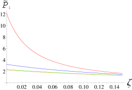
Figure 1: (Color online) The plot of $\tilde{P}_{1}(\zeta)$ (Eq. (53)) for $\gamma=1,\Omega_{0}=2$, corresponding to environmental correlation function $\beta(t)=\nu^{2}{\rm e}^{-Rt}$ for $\nu=1$ and $R=0.1,1,10,100$ represented respectively by the red, blue, green, and orange curves.

Hence, we restrict the illustration of Eqs. (53) to some arbitrary examples of the environmental correlation function. In Fig. 1 we plot the probability of one photon emission, setting $\beta(t)=\nu^{2}{\rm e}^{-Rt}$, which is a standard assumption of the spectral diffusion approach PRL ; JCP . The graph, comparing $\tilde{P}_{1}(\zeta)$ for $R=0.1,1,10,100$ (red, blue, green, orange) shows that an increase in the order of $R$ requires nearly exponential improvement of the measurement accuracy. In Fig. 2 we examine the dependence of the probability of zero photon emission events $\tilde{P}_{0}(\zeta)$ (Fig. 2(b)) on several shapes of $\beta(t)$ (Fig. 2(a)), chosen such that the autocorrelation time $\tau_{c}$ and the maximal value of $\beta(t)$ are close. The fact that for different choices of $\beta(t)$ we arrive at effectively the same result for $\tilde{P}_{0}(\zeta)$ may be seen as a justification of the phenomenological assumption $\beta(t)=\nu^{2}{\rm e}^{-Rt}$, used to plot Fig. 1.

VII $\rm\bf\Large\@slowromancap vii@$ Summary

By superposing an approximate phenomenological Dyson equation with a microscopic reduced master equation, we provided a correspondence between the microscopic and the spectral diffusion approaches. It was shown that excluding the interaction of the two-level system emitter with the laser, the dynamics governed by the spectral diffusion model is indistinguishable from the dynamics obtained by the microscopic theory, whenever the evolution of the environment is not determined on the microscopic level. This allowed to identify, up to a constant, the spectral diffusion correlation function with the real part of the thermal environmental correlation function. Furthermore, it was demonstrated that the real problem of using the spectral diffusion method for the description of standard SMS experiments beyond the Markovian limit, is the independent rates of variation assumption, which can be overcome using the microscopic reduced propagator theory Vega ; DGS ; TYu . Finally, combining the methods of the latter with the generalized generating functions approach, we have established analytic expressions for the thermal correlation function allowing to extract information on the environmental noise beyond the Markovian approximation from the measured single emitter photon statistics.

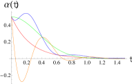
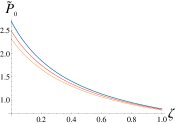
$(a)$	$(b)$

Figure 2: (Color online)(a) The plot of $\beta(t)=A{\rm e}^{-Rt};~{}A{\rm e}^{-Rt^{2}};~{}(1-A\cos[Bt]){\rm e}^{-Rt};~{}(A-\sin[Bt]){\rm e}^{-Rt}$, for $A=0.5$ and $B=10$, represented respectively by the red, blue, green, and orange curves;(b) The plot of $\tilde{P}_{0}(\zeta)$ (Eq. (53)), for $\gamma=1,\Omega_{0}=2$, resulting from a different choice of the environmental correlation function in Fig. 2(b). The colors of the curves are matched .

Appendix A: Derivation of Dyson equation

In this appendix we provide the details of derivation of Eqs. (21,22). Substituting $\vec{\rho}(t|\eta_{t})=\hat{U}(t,t_{0}|\eta_{t})\vec{\rho}(t_{0})$, where $\hat{U}(t,t_{0}|\eta_{t})$ is the propagator, into Eq. (15) we have

$$\frac{d}{dt}\hat{U}(t,t_{0}|\eta_{t})=\ \hat{\cal O}\left[\hat{U}(t,t_{0}|\eta_{t}),t\right]+\eta_{t}\hat{\Upsilon}\hat{U}(t,t_{0}|\eta_{t}),$$ (A.1)

and rewrite the latter equation in the integral form CT

$$\hat{U}(t,t_{0}|\eta_{t})=\hat{U}_{0}(t,t_{0})+\int_{t_{0}}^{t}\hat{U}_{0}(t,\tau)\eta_{\tau}\hat{\Upsilon}\hat{U}(t,t_{0}|\eta_{t})d\tau,$$ (A.2)

where $\hat{U}_{0}(t,t_{0})$ is the solution of Eq. (18). Further, we expand Eq. (A.2) by iteration

$$\!\hat{U}(t,t_{0}|\eta_{t})=\hat{U}_{0}(t,t_{0})+\int_{t_{0}}^{t}dt_{1}\hat{U}_{0}(t,t_{1})\eta_{t_{1}}\hat{\Upsilon}\hat{U}_{0}(t_{1},t_{0})+$$

$$+\int_{t_{0}}^{t}dt_{1}\int_{t_{0}}^{t_{2}}dt_{1}\hat{U}_{0}(t,t_{2})\eta_{t_{2}}\hat{\Upsilon}\hat{U}_{0}(t_{2},t_{1})\eta_{t_{1}}\hat{\Upsilon}\hat{U}_{0}(t_{1},t_{0})+$$

$$\!\!\!\!+\!\int_{t_{0}}^{t}\!\!dt_{3}\!\!\int_{t_{0}}^{t_{3}}\!\!\!dt_{2}\!\!\int_{t_{0}}^{t_{2}}\!\!\!\!\!\!dt_{1}\hat{U}_{0}(t,t_{3})\eta_{t_{3}}\hat{\Upsilon}\hat{U}_{0}(t_{3},t_{2})\eta_{t_{2}}\hat{\Upsilon}\times$$

$$\times\hat{U}_{0}(t_{2},t_{1})\eta_{t_{1}}\hat{\Upsilon}\hat{U}_{0}(t_{1},t_{0})+$$

$$\!\!+\!\int_{t_{0}}^{t}\!\!\!dt_{4}\!\!\int_{t_{0}}^{t_{4}}\!\!\!dt_{3}\!\!\int_{t_{0}}^{t_{3}}\!\!\!dt_{2}\!\!\int_{t_{0}}^{t_{2}}\!\!\!dt_{1}\hat{U}_{0}(t,t_{4})\eta_{t_{4}}\hat{\Upsilon}\hat{U}_{0}(t_{4},t_{3})\times$$

$$\times\eta_{t_{3}}\hat{\Upsilon}\hat{U}_{0}(t_{3},t_{2})\eta_{t_{2}}\hat{\Upsilon}\hat{U}_{0}(t_{2},t_{1})\eta_{t_{1}}\hat{\Upsilon}\hat{U}_{0}(t_{1},t_{0})+...~{}.$$ (A.3)

Assuming $\eta_{t}$ is a zero mean Gaussian noise, we take an average of Eq. (A.3). Discarding the long time correlations contribution, as discussed in Section $\rm\@slowromancap iii@$, this gives

$$\!\hat{U}(t,t_{0})=\hat{U}_{0}(t,t_{0})+$$

$$+\int_{t_{0}}^{t}dt_{1}\int_{t_{0}}^{t_{2}}dt_{1}\langle\eta_{t_{2}}\eta_{t_{1}}\rangle\hat{U}_{0}(t,t_{2})\hat{\Upsilon}\hat{U}_{0}(t_{2},t_{1})\hat{\Upsilon}\hat{U}_{0}(t_{1},t_{0})+$$

$$\!\!+\!\int_{t_{0}}^{t}\!\!\!dt_{4}\!\!\int_{t_{0}}^{t_{4}}\!\!\!dt_{3}\!\!\int_{t_{0}}^{t_{3}}\!\!\!dt_{2}\!\!\int_{t_{0}}^{t_{2}}\!\!\!dt_{1}\langle\eta_{t_{4}}\eta_{t_{3}}\rangle\langle\eta_{t_{2}}\eta_{t_{1}}\rangle\hat{U}_{0}(t,t_{4})\times$$

$$\times\hat{\Upsilon}\hat{U}_{0}(t_{4},t_{3})\hat{\Upsilon}\hat{U}_{0}(t_{3},t_{2})\hat{\Upsilon}\hat{U}_{0}(t_{2},t_{1})\hat{\Upsilon}\hat{U}_{0}(t_{1},t_{0})+...,$$ (A.4)

where $\hat{U}(t,t_{0})=\langle\hat{U}(t,t_{0}|\eta_{t})\rangle$. Evidently, the above iterative expansion is equivalent to

$$\!\hat{U}(t,t_{0})=\hat{U}_{0}(t,t_{0})+$$

$$+\int_{t_{0}}^{t}dt_{1}\int_{t_{0}}^{t_{2}}dt_{1}\langle\eta_{t_{2}}\eta_{t_{1}}\rangle\hat{U}_{0}(t,t_{2})\hat{\Upsilon}\hat{U}_{0}(t_{2},t_{1})\hat{\Upsilon}\hat{U}(t_{1},t_{0}),$$ (A.5)

which in turn, by analogy with Eqs. (A.1,A.2), is equivalent to the differential equation

$$\!\!\frac{d}{dt}\hat{U}(t,t_{0})\!=\!\hat{\cal O}\left[\hat{U}(t,t_{0}),t\right]\!+\!\int_{t_{0}}^{t}\!\!d\tau\langle\eta_{t}\eta_{\tau}\rangle\hat{\Upsilon}\hat{U}_{0}(t,t_{\tau})\hat{\Upsilon}\hat{U}(t_{\tau},t_{0}).$$ (A.6)

Finally, acting with the last equation on the initial state $\vec{\rho}(t_{0})$ yields Eqs. (21,22).

Appendix B: Reduced propagators approach with two reservoirs

In this appendix we consider a closed system, composed of a two-level particle interacting with a thermal reservoir, a monochromatic laser field and the electromagnetic vacuum. The total Hamiltonian within the rotating wave approximation (RWA) with respect to the coupling to the electromagnetic field is CT ; Scully ; Vega ; DGS ; TYu

$$\begin{array}[]{c}\hat{H}(t)=\frac{\omega_{0}}{2}\hat{\sigma}_{z}+(\hat{\sigma}_{+}\frac{\Omega_{0}}{2}{\rm e}^{-i\omega_{L}t}+\hat{\sigma}_{-}\frac{\Omega_{0}}{2}{\rm e}^{i\omega_{L}t})+\\ \\ +\sum_{\lambda}\omega_{\lambda}\hat{b}^{{\dagger}}_{\lambda}\hat{b}_{\lambda}+\sum_{\mu}\omega_{\mu}\hat{a}^{{\dagger}}_{\mu}\hat{a}_{\mu}+\\ \\ +\sum_{\lambda}g_{\lambda}\hat{\sigma}_{z}(\hat{b}^{{\dagger}}_{\lambda}+\hat{b}_{\lambda})+\sum_{\mu}p_{\mu}(\hat{\sigma}_{+}\hat{a}_{\mu}+\hat{\sigma}_{-}\hat{a}^{{\dagger}}_{\mu}),\end{array}$$ (B.1)

where $\hat{b}^{{\dagger}}_{\lambda},\hat{b}_{\lambda}$ and $\hat{a}^{{\dagger}}_{\lambda},\hat{a}_{\lambda}$ are the boson ladder operators of the thermal environment and the electromagnetic field respectively, the Pauli matrices $\hat{\sigma}_{i}$ represent the particle operators, and $\Omega_{0}$ is the Rabi frequency of the laser pump oscillating at frequency $\omega_{L}$. Transforming to the rotating frame by

$$\hat{R}(t)=\exp\left[i\frac{\omega_{L}}{2}t\hat{\sigma}_{z}+\sum_{\mu}i\omega_{L}t\hat{a}^{{\dagger}}_{\mu}\hat{a}_{\mu}\right],$$ (B.2)

we suppress the time dependence in Eq. (B.1), which yields Eq. (34) of the article.

Given Eq. (34), extending the methods of Vega ; DGS ; TYu for simultaneous interaction of the particle with two bosonic reservoirs, we consider the total propagator of the system in the partial representation picture with respect to $\hat{H}_{B}+\hat{H}_{R}=\sum_{\lambda}\omega_{\lambda}\hat{b}^{{\dagger}}_{\lambda}\hat{b}_{\lambda}+\sum_{\mu}(\omega_{\mu}-\omega_{L})\hat{a}^{{\dagger}}_{\mu}\hat{a}_{\mu}$:

$$\hat{U}_{I}(t,{t_{0}})={\rm e}^{i(\hat{H}_{B}+\hat{H}_{R})(t-t_{0})}\hat{U}(t-{t_{0}}){\rm e}^{-i(\hat{H}_{B}+\hat{H}_{R})(t-t_{0})},$$ (B.3)

and define the reduced propagator

$$\hat{G}(\vec{y}_{t}^{*}\vec{z}_{t}^{*}\vec{y}_{t_{0}}\vec{z}_{t_{0}}|tt_{0})\equiv\langle\vec{y}_{t}\vec{z}_{t}|\hat{U}_{I}(t,{t_{0}})|\vec{y}_{t_{0}}\vec{z}_{t_{0}}\rangle,$$ (B.4)

where $|\vec{z}_{t}\rangle=\prod_{\lambda}|z_{t,\lambda}\rangle$ describes the thermal field in the Bargmann coherent states representation (and similarly, $|\vec{y}_{t}\rangle$ represents the state of the electromagnetic field). Applying $\hat{G}(\vec{y}_{t}^{*}\vec{z}_{t}^{*}\vec{y}_{t_{0}}\vec{z}_{t_{0}}|tt_{0})$ to the initial state of the two-level system, propagates the latter such that the final state is simultaneously conditioned by specific evolution trajectories of both reservoirs. In what follows we show that under certain circumstances, the particle conditional density matrix $\hat{\rho}_{I}(\vec{y}_{t}^{*}\vec{z}_{t}^{*}\vec{y}_{t_{0}}\vec{z}_{t_{0}}|tt_{0})$ depends on the environmental degrees of freedom through the stochastic processes $y_{t},z_{t}$ and their autocorrelation functions $\alpha(t),\beta(t)$, defined below. This constitutes a simplification of the general case, where higher order cross-correlation functions of $y_{t}$ and $z_{t}$ can be involved as well.

The time evolution equation for $\hat{G}(\vec{y}_{t}^{*}\vec{z}_{t}^{*}\vec{y}_{t_{0}}\vec{z}_{t_{0}}|tt_{0})$ is obtained from the projection of the Schrödinger equation for $\hat{U}_{I}(t,t_{0})$, given by Eq. (B.3):

$$\begin{array}[]{c}\frac{\partial}{\partial t}\hat{G}(\vec{y}_{t}^{*}\vec{z}_{t}^{*}\vec{y}_{t_{0}}\vec{z}_{t_{0}}|tt_{0})=\langle\vec{y}_{t}\vec{z}_{t}|\frac{\partial}{\partial t}\hat{U}_{I}(t,{t_{0}})|\vec{y}_{t_{0}}\vec{z}_{t_{0}}\rangle=\\ \\ =-i\left[\hat{H}_{S}+\hat{\sigma}_{z}\sum_{\lambda}g_{\lambda}{\rm e}^{i\omega_{\lambda}t}z_{t,\lambda}^{*}+\right.\\ \\ \left.+\hat{\sigma}_{-}\sum_{\mu}p_{\mu}{\rm e}^{i(\omega_{\mu}-\omega_{L})t}y_{t,\mu}^{*}\right]\hat{G}(\vec{y}_{t}^{*}\vec{z}_{t}^{*}\vec{y}_{t_{0}}\vec{z}_{t_{0}}|tt_{0})-\\ \\ -i\hat{\sigma}_{z}\sum_{\lambda}g_{\lambda}{\rm e}^{-i\omega_{\lambda}t}\langle\vec{y}_{t}\vec{z}_{t}|\hat{b}_{\lambda}\hat{U}_{I}(t,{t_{0}})|\vec{y}_{{t_{0}}}\vec{z}_{{t_{0}}}\rangle-\\ \\ -i\hat{\sigma}_{+}\sum_{\mu}p_{\mu}{\rm e}^{-i(\omega_{\mu}-\omega_{L})t}\langle\vec{y}_{t}\vec{z}_{t}|\hat{a}_{\mu}\hat{U}_{I}(t,{t_{0}})|\vec{y}_{t_{0}}\vec{z}_{t_{0}}\rangle,\end{array}$$ (B.5)

where the last two terms constitute an obstacle for getting a closed equation for $\hat{G}(\vec{y}_{t}^{*}\vec{z}_{t}^{*}\vec{y}_{t_{0}}\vec{z}_{t_{0}}|tt_{0})$. We use the same scheme as above to represent these terms as functions of $\hat{G}(\vec{y}_{t}^{*}\vec{z}_{t}^{*}\vec{y}_{t_{0}}\vec{z}_{t_{0}}|tt_{0})$. Starting with the thermal reservoir we have

$$\begin{array}[]{c}\langle\vec{y}_{t}\vec{z}_{t}|\hat{b}_{\lambda}\hat{U}_{I}(t,{t_{0}})|\vec{y}_{t_{0}}\vec{z}_{t_{0}}\rangle=\\ \\ =\langle\vec{y}_{t}\vec{z}_{t}|\hat{U}_{I}(t,{t_{0}})\hat{U}_{I}^{-1}(t,{t_{0}})\hat{b}_{\lambda}\hat{U}_{I}(t,{t_{0}})|\vec{y}_{t_{0}}\vec{z}_{t_{0}}\rangle=\\ \\ =\langle\vec{y}_{t}\vec{z}_{t}|\hat{U}_{I}(t,{t_{0}})\hat{b}_{\lambda}(t,{t_{0}})|\vec{y}_{t_{0}}\vec{z}_{t_{0}}\rangle,\end{array}$$ (B.6)

where

$$\hat{b}_{\lambda}(t,{t_{0}})\equiv\hat{U}_{I}^{-1}(t,{t_{0}})\hat{b}_{\lambda}\hat{U}_{I}(t,{t_{0}}).$$ (B.7)

Rewriting Eq. (B.7) in the integral form yields

$$\hat{b}_{\lambda}(t,{t_{0}})=\hat{b}_{\lambda}-ig_{\lambda}\int_{t_{0}}^{t}\hat{\sigma}_{z}(\tau,{t_{0}}){\rm e}^{i\omega_{\lambda}\tau}d\tau,$$ (B.8)

where $\hat{\sigma}_{z}(\tau,{t_{0}})=\hat{U}_{I}^{-1}(t,{t_{0}})\hat{\sigma}_{z}\hat{U}_{I}(t,{t_{0}})$. Repeating the same procedure with respect to the radiation field and inserting the results back into Eq. (B.5) gives

$$\begin{array}[]{c}\frac{\partial}{\partial t}\hat{G}(\vec{y}_{t}^{*}\vec{z}_{t}^{*}\vec{y}_{t_{0}}\vec{z}_{t_{0}}|tt_{0})=\left[-i\hat{H}_{S}+\hat{\sigma}_{z}z_{t}^{*}-\hat{\sigma}_{z}z_{t_{0}}+\right.\\ \\ \left.+\hat{\sigma}_{-}y_{t}^{*}-\hat{\sigma}_{+}y_{t_{0}}\right]\hat{G}(\vec{y}_{t}^{*}\vec{z}_{t}^{*}\vec{y}_{t_{0}}\vec{z}_{t_{0}}|tt_{0})-\\ \\ -i\hat{\sigma}_{z}\int_{t_{0}}^{t}\beta(t-\tau)\langle\vec{y}_{t}\vec{z}_{t}|\hat{U}_{I}(t,t_{0})\hat{\sigma}_{z}(\tau,t_{0})|\vec{y}_{t_{0}}\vec{z}_{t_{0}}\rangle d\tau-\\ \\ -i\hat{\sigma}_{+}\int_{t_{0}}^{t}\alpha(t-\tau)\langle\vec{y}_{t}\vec{z}_{t}|\hat{U}_{I}(t,t_{0})\hat{\sigma}_{-}(\tau,t_{0})|\vec{y}_{t_{0}}\vec{z}_{t_{0}}\rangle d\tau,\end{array}$$ (B.9)

where

$$z_{\tau}\equiv-i\sum_{\lambda}g_{\lambda}{\rm e}^{i\omega_{\lambda}t}z_{\tau,\lambda},~{}y_{\tau}\equiv-i\sum_{\mu}p_{\mu}{\rm e}^{i(\omega_{\mu}-\omega_{L})t}y_{\tau,\mu},$$ (B.10)

and

$$\beta(t)\equiv\sum_{\lambda}|g_{\lambda}|^{2}{\rm e}^{-i\omega_{\lambda}t},~{}\alpha(t)\equiv\sum_{\mu}|p_{\mu}|^{2}{\rm e}^{-i(\omega_{\mu}-\omega_{L})t}.\\$$ (B.11)

Further, in order to close Eq. (B.9), we are interested in rearranging the last two terms in Eq. (B.9) as

$$\begin{array}[]{c}\!\!\!\!\langle\vec{y}_{t}\vec{z}_{t}|\hat{U}_{I}(t,{t_{0}})\hat{\sigma}_{i}(\tau,{t_{0}})|\vec{y}_{t_{0}}\vec{z}_{t_{0}}\rangle\!=\!\langle\vec{y}_{t}\vec{z}_{t}|\hat{\sigma}_{i}(\tau,t)\hat{U}_{I}(t,{t_{0}})|\vec{y}_{t_{0}}\vec{z}_{t_{0}}\rangle\\ \\ =\hat{O}(y^{*}_{t}z^{*}_{t}y_{t_{0}}z_{t_{0}}t\tau)\hat{G}(\vec{y}^{*}_{t}\vec{z}_{t}^{*}\vec{y}_{t_{0}}\vec{z}_{t_{0}}|t{t_{0}}),\end{array}$$ (B.12)

where $\hat{O}(y^{*}_{t}z^{*}_{t}y_{t_{0}}z_{t_{0}}t\tau)$ is an operator acting in the particle subspace. This can be done by formally integrating and iterating the Heisenberg equation for $\hat{\sigma}_{i}(\tau,t)$ in power series of $g_{\lambda}$ and $p_{\mu}$. Taking into account that the autocorrelation functions $\alpha(t),\beta(t)$ are already of the second order in $g_{\lambda}$ and $p_{\mu}$ respectively, keeping only the zeroth order solution for $\hat{\sigma}_{i}(\tau,t)$:

$$\hat{\sigma}_{i}(\tau,t)={\rm e}^{-iH_{S}(t-\tau)}\hat{\sigma}_{i}{\rm e}^{iH_{S}(t-\tau)}+{\cal O}(g)$$ (B.13)

accounts for a satisfactory approximation in the case $g_{\lambda}$ and $p_{\mu}$ are small. Substituting the truncated expansion Eq. (B.13) back into Eq. (B.9) we neglect all the terms proportional to $g_{\lambda}^{n}p_{\mu}^{m}$ with $m+n>2$. Since the zeroth order approximation Eq. (B.13) is restricted to the particle subspace, we can pull it out of the brackets in Eq. (B.12), which allows to close the equation for $\hat{G}(\vec{y}^{*}_{t}\vec{z}_{t}^{*}\vec{y}_{t_{0}}\vec{z}_{t_{0}}|t{t_{0}})$ and yields

$$\begin{array}[]{c}\frac{\partial}{\partial t}\hat{G}(\vec{y}^{*}_{t}\vec{z}_{t}^{*}\vec{y}_{t_{0}}\vec{z}_{t_{0}}|t{t_{0}})=\\ \\ =\left[-i\hat{H}_{S}+\hat{\sigma}_{z}z_{t}^{*}-\hat{\sigma}_{z}z_{t_{0}}+\hat{\sigma}_{-}y_{t}^{*}-\hat{\sigma}_{+}y_{t_{0}}\right.-\\ \\ -i\hat{\sigma}_{z}\int_{t_{0}}^{t}\beta(t-\tau){\rm e}^{-i\hat{H}_{S}(t-\tau)}\hat{\sigma}_{z}{\rm e}^{i\hat{H}_{S}(t-\tau)}-\\ \\ \left.-i\hat{\sigma}_{+}\int_{t_{0}}^{t}\alpha(t-\tau){\rm e}^{-i\hat{H}_{S}(t-\tau)}\hat{\sigma}_{-}{\rm e}^{i\hat{H}_{S}(t-\tau)}\right]\times\\ \\ \times\hat{G}(\vec{y}^{*}_{t}\vec{z}_{t}^{*}\vec{y}_{t_{0}}\vec{z}_{t_{0}}|t{t_{0}})d\tau.\end{array}\\$$ (B.14)

The lesson of Eq. (B.14) is that within the second order approximation in the interaction magnitudes, the effective coupling between the two reservoirs is eliminated. The reduced evolution of the particle is given by direct independent summation of the contribution arising from the interaction with each one of the fields alone.

From now on the results of Vega ; DGS ; TYu may be adopted directly. Using Eq. (B.14) the master equation for the conditional density matrix follows from

$$\begin{array}[]{c}\frac{\partial}{\partial t}\hat{\rho}_{I}(\vec{y}^{*}_{t}\vec{z}^{*}_{t}\vec{y}_{t_{0}}\vec{z}_{t_{0}}|tt_{0})=\frac{\partial}{\partial t}\left[\hat{G}(\vec{y}^{*}_{t}\vec{z}_{t}^{*}\vec{y}_{t_{0}}\vec{z}_{t_{0}}|t{t_{0}})\times\right.\\ \\ \left.\times\hat{\rho}_{I}(\vec{y}^{*}_{t_{0}}\vec{z}^{*}_{t_{0}}\vec{y}_{t_{0}}\vec{z}_{t_{0}}|t_{0}t_{0})\hat{G}(\vec{y}^{*}_{t}\vec{z}_{t}^{*}\vec{y}_{t_{0}}\vec{z}_{t_{0}}|t{t_{0}})\right].\end{array}$$ (B.15)

Afterwards, the evolution equation for the marginal density matrix $\hat{\rho}_{S}(t)$ is obtained by integrating out the irrelevant environmental degrees of freedom, taking into account the initial Boltzmann equilibrium distribution of the thermal bath and the zero temperature $\delta$-correlated distribution of the electromagnetic vacuum. This procedure, requiring an application of the generalized Novikov theorem, was worked out in Vega ; DGS ; TYu . Using the results for each of the two reservoirs respectively we obtain Eq. (35).

References

• (1) C.K. Hong, Z. Y. Ou, L. Mandel Phys. Rev. Lett. 59, 2044-2046 (1987).
• (2) E. Knill, R. Laflamme and G. J. Milburn Nature 409, 46-52 (2001).
• (3) Y.H. Shih, C. O. Alley Phys. Rev. Lett. 61, 2921-2024 (1988).
• (4) D. Bouwmeester, A. Ekert, A. Zelinger the Physics of Quantum Information49-92 Springer, Berlin (2000).
• (5) Erik M.H.P van Dijk et al Phys. Rev. Lett. 94, 078302 (2005).
• (6) C. Santori, D. Fattal, J. Vu$\hat{c}$kovi$\acute{c}$, G. S. Solomon and Y. Yamamoto Nature 419, 594-597 (2002).
• (7) N. Katz, M. Ansmann, R. C. Bialczak, E. Lucero, R. McDermott, M. Neeley, M. Steffen, E. M. Weig, A. N. Korotkov Sience 312, 1498-1500 (2006).
• (8) C. Brunel, B. Lounis, P. Tamarat and M. Orrit Phys. Rev. Lett. 83, 2722 (1999).
• (9) A.O. Caldeira, A.J. Leggett, Physica A 121, 587 (1983).
• (10) L. Diósi Physica A 199, 517 (1993).
• (11) R. Kubo, M. Toda, and N. Hashitsume, “Statistical Physics Vol. 2.”, Springer, Berlin, (1995).
• (12) H. Mori, Progr. Theor. Phys. 33, 423 (1965).
• (13) R. Zwanzig, J. Chem. Phys 33, 1338 (1960).
• (14) R. Zwanzig Jour. Stat. Phys. 9, 215 (1973).
• (15) S. Nakajima, Prog. Theor. Phys. 20, 948 (1958).
• (16) C. Cohen-Tannoudji, J. Dupont-Roc, G. Girynberg, “Atom-Photon Interactions”, A Willey-Interscience Publishion, (1992).
• (17) U. Weiss, “Quantum Dissipative Systems”, World Scientific Publishing , (1999).
• (18) M. O. Scully, M. S. Zubairy, “Quantum Optics”, Cambridge University Press , (1997).
• (19) I. de Vega , D. Alonso, P. Gaspard, W. T. Strunz, Jour. Chem. Phys., 1225, 1, (2005); I. de Vega, D. Alonso, Phys. Rev. A, 73, 022102 (2006); I. de Vega, D. Alonso, P. Gaspard, Phys. Rev. A, 71, 023812 (2005); D. Alonso, I. De Vega, E. Hernandez-Concepción, Comptes Rendus Physique 8, 684-695, (2007); ftp://tesis.bbtk.ull.es/ccppytec/cp256.pdf
• (20) L. Diósi, N. Gisin, and W. T. Strunz, Phys. Rev. A 58, 1699 (1998).
• (21) T. Yu, L. Diósi, N. Gisin, and W. T. Strunz, Phys. Rev. A 60, 91 (1999).
• (22) http://www.rp-photonics.com/photonic_crystal_fibers.html
• (23) Y. Zheng, F. L. H. Brown Phys. Rev. Lett. 90, 238305 (2003).
• (24) F. Shikerman, E. Barkai Phys. Rev. Lett. 99, 208302 (2007).
• (25) F. Shikerman, E. Barkai Jour. Chem. Phys. 129, 244702 (2008).
• (26) H. Risken “The Fokker-Plank Equation”, Springer-Verlag, Berlin, (1984).
• (27) M. B. Plenio and P. L. Knight, Rev. of Mod. Phys. 70, 101-144 (1998).
• (28) A. A. Budini Jour. Chem. Phys 126, 054101 (2007).
• (29) L. Mandel and E. Wolf, “Optical Coherence and Quantum Optics”, Cambridge University Press, New York, (1995).
• (30) S. Mukamel, “Principles of Nonlinear Optical Spectroscopy”, Oxford University Press, Oxford, (1995).