Comments on Proakis’ Analysis of the Characteristic Function of Complex Gaussian Quadratic Forms

Abstract

An analysis of the characteristic function of Gaussian quadratic forms is presented in [1] to study the performance of multichannel communication systems. This technical report reviews this analysis, obtaining alternative expressions to original ones in compact matrix format.

I Introduction

Statistics of complex Gaussian quadratic forms are a powerful mathematical tool when dealing with digital communications problems. Currently, they are widely used to analyze the performance of digital modulations over fading channels [2]-[8]. In [1] is presented an analysis of one statistic of complex Gaussian quadratic forms which is a very interesting and useful tool to calculate error rates. This analysis, based on the characteristic function of Gaussian quadratic forms, provides a set of expressions which is applicable to a good deal of digital communications problems. To provide a few examples, these expressions have been used to obtain closed-form bit error rate (BER) results in fading channels for multichannel binary signals [2]-[5], quadrature-amplitude modulation (QAM) [6], orthogonal-frequency-division-multiplexing (OFDM) [7], and non-orthogonal multi-pulse modulation (NMM) [8]. In addition, the results presented in [1] are also used to analyze other statistics of complex Gaussian quadratic forms in [9].

In this document is performed a revision to the analysis of the characteristic function of complex gaussian quadratic forms presented in [1]. Alternative expressions in compact matrix format are derived and little mistakes in the original ones has been detected. Up until now, research based on the original expressions has yielded valid results because it dealt with cases where the original and corrected expressions give the same results. However, future uses of the original expressions could lead to wrong results. After deriving alternative expressions, a simple example is presented to confirm the validity of the corrected expressions.

The remainder of this document is organized as follows: Section II states the general problem dealt with herein; Section III describes the alternative analysis which gives the new expressions and detects the mistakes in the original expressions; Section IV presents the aforementioned example which confirms the validity of the new ones; and conclusions are provided in section V.

II General problem statement

The decision variable at the detector of several communication systems, e.g., those employing multichannel binary signals [1], can be expressed as a sum of quadratic forms

$$\begin{split}D&\triangleq\sum\limits_{k=1}^{L}{d_{k}}=\sum\limits_{k=1}^{L}{\mathbf{z}}_{k}^{{\mathcal{H}}}{\mathbf{Qz}}_{k}\\ &=\sum\limits_{k=1}^{L}A\left|{X_{k}}\right|^{2}+B\left|{Y_{k}}\right|^{2}+CX_{k}Y_{k}^{*}+C^{*}X_{k}^{*}Y,\end{split}$$ (1)

with

$${\mathbf{z}}_{k}\triangleq\left[{\begin{array}[]{*{20}c}{X_{k}}\\ {Y_{k}}\\ \end{array}}\right]\quad,\quad{\mathbf{Q}}\triangleq\left[{\begin{array}[]{*{20}c}A&{C^{*}}\\ C&B\\ \end{array}}\right]\quad,\quad d_{k}\triangleq{\mathbf{z}}_{k}^{{\mathcal{H}}}{\mathbf{Qz}}_{k},$$ (2)

where $\mathbf{Q}$ is a Hermitian matrix and $X_{k}$, $Y_{k}$ complex circularly-symmetric Gaussian random variables. The set of vectors $\{{\mathbf{z}}_{k}\}_{k=1,...,L}$ are mutually statistically independent with a different mean ${\mathbf{m}}_{k}$ but identical non-singular covariance matrix $\mathbf{R}$, respectively defined as

$${\mathbf{m}}_{k}\triangleq\left[{\begin{array}[]{*{20}c}{\bar{X}_{k}}\\ {\bar{Y}_{k}}\\ \end{array}}\right]\quad,\quad{\mathbf{R}}\triangleq{\text{E}}\left\{{({\mathbf{z}}_{k}-{\mathbf{m}}_{k})({\mathbf{z}}_{k}-{\mathbf{m}}_{k})^{\mathcal{H}}}\right\}.$$ (3)

The constants $A$, $B$ and $C$ must be appropriately identified with the specific parameters of the problem, so that $D$ characterizes the decision variable at the output of the detector to further calculate the probability of error as $\Pr\{D<0\}$. This calculation leads to non-trivial results when $\mathbf{Q}$ is indefinite, i.e., when $\left|C\right|^{2}-AB>0$, because otherwise the probability $\Pr\{D<0\}$ will be either 0 or 1. Note that indefiniteness for $2\times 2$ matrices implies non-singularity.

An expression for the probability $\Pr\{D<0\}$ is derived in [1] using the characteristic function of $D$, denoted as $\phi_{D}(\upsilon)$. In this derivation, mutual independence of the terms $d_{k}$ in (1) is used, thus, the function $\phi_{D}(\upsilon)$ can be expressed as the product of the characteristic functions $\phi_{k}$ of each summand, i.e.,

$$\phi_{D}(\upsilon)\triangleq{\text{E}}\left\{{e^{j\upsilon D}}\right\}=\prod\limits_{k=1}^{L}{\phi_{k}(\upsilon)},$$ (4)

with

$$\phi_{k}(\upsilon)=\frac{{v_{1}v_{2}}}{{\left({\upsilon+jv_{1}}\right)\left({\upsilon-jv_{2}}\right)}}\exp\left({\frac{{v_{1}v_{2}\left({-\upsilon^{2}\alpha_{1k}+j\upsilon\alpha_{2k}}\right)}}{{\left({\upsilon+jv_{1}}\right)\left({\upsilon-jv_{2}}\right)}}}\right).$$ (5)

The first two columns of table II lists the parameters $v_{1}$, $v_{2}$, $\alpha_{1k}$, $\alpha_{2k}$, as well as other intermediate definitions and the expression of the probability $\Pr\{D<0\}$ derived in [1]. In the table, $Q_{1}$ and $I_{n}$ are the first-order Marcum Q-function and the modified Bessel function of the first kind, respectively.

TABLE I: Expressions of the error rate for binary signals

Parameter	Proakis’ Definition	Correction
$\mu_{xy}$	$\frac{1}{2}{\text{E}}\left\{{\left({X_{k}-\bar{X}_{k}}\right)\left({Y_{k}-\bar{Y}_{k}}\right)^{*}}\right\}$
$w$	$\dfrac{{A\mu_{xx}+B\mu_{yy}+C\mu_{xy}^{*}+C^{*}\mu_{xy}}}{{4(\mu_{xx}\mu_{yy}-\left|{\mu_{xy}}\right|^{2})(\left|C\right|^{2}-AB)}}$	$\dfrac{{A\mu_{xx}+B\mu_{yy}+C^{*}\mu_{xy}^{*}+C\mu_{xy}}}{{4(\mu_{xx}\mu_{yy}-\left|{\mu_{xy}}\right|^{2})(\left|C\right|^{2}-AB)}}$
$v_{1}$	$\sqrt{w^{2}+\dfrac{1}{{4(\mu_{xx}\mu_{yy}-\left|{\mu_{xy}}\right|^{2})(\left|C\right|^{2}-AB)}}}-w$
$v_{2}$	$\sqrt{w^{2}+\dfrac{1}{{4(\mu_{xx}\mu_{yy}-\left|{\mu_{xy}}\right|^{2})(\left|C\right|^{2}-AB)}}}+w$
$\alpha_{1k}$	$2\left({\left|C\right|^{2}-AB}\right)\left({\left|{\bar{X}_{k}}\right|^{2}\mu_{yy}+\left|{\bar{Y}_{k}}\right|^{2}\mu_{xx}-\bar{X}_{k}^{*}\bar{Y}_{k}\mu_{xy}-\bar{X}_{k}\bar{Y}_{k}^{*}\mu_{xy}^{*}}\right)$
$\alpha_{2k}$	$A\left|{\bar{X}_{k}}\right|^{2}+B\left|{\bar{Y}_{k}}\right|^{2}+C\bar{X}_{k}^{*}\bar{Y}_{k}+C^{*}\bar{X}_{k}\bar{Y}_{k}^{*}$	$A\left|{\bar{X}_{k}}\right|^{2}+B\left|{\bar{Y}_{k}}\right|^{2}+C^{*}\bar{X}_{k}^{*}\bar{Y}_{k}+C\bar{X}_{k}\bar{Y}_{k}^{*}$
$\alpha_{1}$	$\sum\nolimits_{k=1}^{L}{\alpha_{1k}}$
$\alpha_{2}$	$\sum\nolimits_{k=1}^{L}{\alpha_{2k}}$
$a$	$\left[{\dfrac{{2v_{1}^{2}v_{2}\left({\alpha_{1}v_{2}-\alpha_{2}}\right)}}{{\left({v_{1}+v_{2}}\right)^{2}}}}\right]^{1/2}$
$b$	$\left[{\dfrac{{2v_{1}v_{2}^{2}\left({\alpha_{1}v_{1}+\alpha_{2}}\right)}}{{\left({v_{1}+v_{2}}\right)^{2}}}}\right]^{1/2}$
$\Pr\{D<0\}$	$\begin{gathered}Q_{1}(a,b)-I_{0}(ab)\exp\left\{{-\frac{1}{2}(a^{2}+b^{2})}\right\}+\frac{{I_{0}(ab)\exp\left\{{-\frac{1}{2}(a^{2}+b^{2})}\right\}}}{{(1+v_{2}/v_{1})^{2L-1}}}\sum\limits_{k=0}^{L-1}{\left({\begin{array}[]{*{20}c}{2L-1}\\ k\\ \end{array}}\right)\left({\frac{{v_{2}}}{{v_{1}}}}\right)^{k}}\hfill\\ +\frac{{\exp\left\{{-\frac{1}{2}(a^{2}+b^{2})}\right\}}}{{(1+v_{2}/v_{1})^{2L-1}}}\sum\limits_{n=1}^{L-1}{I_{n}(ab)}\sum\limits_{k=0}^{L-1-n}{\left({\begin{array}[]{*{20}c}{2L-1}\\ k\\ \end{array}}\right)}\left[{\left({\frac{b}{a}}\right)^{n}\left({\frac{{v_{2}}}{{v_{1}}}}\right)^{k}-\left({\frac{a}{b}}\right)^{n}\left({\frac{{v_{2}}}{{v_{1}}}}\right)^{2L-1-k}}\right]\hfill\\ \end{gathered}$
$\begin{gathered}\Pr\{D<0\}\\ (L=1)\hfill\end{gathered}$	$Q_{1}(a,b)-\dfrac{{v_{2}/v_{1}}}{{1+v_{2}/v_{1}}}I_{0}(ab)\exp\left\{{-\frac{1}{2}(a^{2}+b^{2})}\right\}$

TABLE II: Alternative expressions of the error rate for binary signals

Parameter	Definition
$\delta_{1}$	positive eigenvalue of $\mathbf{RQ}$
$\delta_{2}$	negative eigenvalue of $\mathbf{RQ}$
$a$	$\sqrt{\dfrac{{2\delta_{2}\left({\sum\nolimits_{k=1}^{L}{{\mathbf{m}}_{k}^{H}\left[{\mathbf{Q}}-\delta_{1}{\mathbf{R}^{-1}}\right]{\mathbf{m}}_{k}}}\right)}}{{\left({\delta_{1}-\delta_{2}}\right)^{2}}}}$
$b$	$\sqrt{\dfrac{{2\delta_{1}\left({\sum\nolimits_{k=1}^{L}{{\mathbf{m}}_{k}^{H}\left[{\mathbf{Q}}-\delta_{2}{\mathbf{R}^{-1}}\right]{\mathbf{m}}_{k}}}\right)}}{{\left({\delta_{1}-\delta_{2}}\right)^{2}}}}$
$\Pr\{D<0\}$	$\begin{gathered}Q_{1}(a,b)-I_{0}(ab)\exp\left\{{-\frac{1}{2}(a^{2}+b^{2})}\right\}+\frac{{I_{0}(ab)\exp\left\{{-\frac{1}{2}(a^{2}+b^{2})}\right\}}}{{(1-\delta_{1}/\delta_{2})^{2L-1}}}\sum\limits_{k=0}^{L-1}{\left({\begin{array}[]{*{20}c}{2L-1}\\ k\\ \end{array}}\right)\left|{\frac{{\delta_{1}}}{{\delta_{2}}}}\right|^{k}}\hfill\\ +\frac{{\exp\left\{{-\frac{1}{2}(a^{2}+b^{2})}\right\}}}{{(1-\delta_{1}/\delta_{2})^{2L-1}}}\sum\limits_{n=1}^{L-1}{I_{n}(ab)}\sum\limits_{k=0}^{L-1-n}{\left({\begin{array}[]{*{20}c}{2L-1}\\ k\\ \end{array}}\right)}\left[{\left({\frac{b}{a}}\right)^{n}\left|{\frac{{\delta_{1}}}{{\delta_{2}}}}\right|^{k}-\left({\frac{a}{b}}\right)^{n}\left|{\frac{{\delta_{1}}}{{\delta_{2}}}}\right|^{2L-1-k}}\right]\hfill\\ \end{gathered}$
$\begin{gathered}\Pr\{D<0\}\\ (L=1)\hfill\end{gathered}$	$Q_{1}(a,b)+\dfrac{{\delta_{1}}}{{\delta_{2}-\delta_{1}}}I_{0}(ab)\exp\left\{{-\frac{1}{2}(a^{2}+b^{2})}\right\}$

III Alternative analysis

An alternative formulation of the characteristic function $\phi_{k}$ is used in this section to obtain new expressions for the probability $\Pr\{D<0\}$.

In [10], Turin deducts the following expression for the characteristic function of a quadratic form of $n$ variables $\mathbf{z}^{\mathcal{H}}\mathbf{Qz}$

$$\phi(\upsilon)=\frac{{\exp\left({-{\mathbf{m}}^{\mathcal{H}}{\mathbf{R}}^{-1}\left[{{\mathbf{I}}-({\mathbf{I}}-j\upsilon{\mathbf{RQ}})^{-1}}\right]{\mathbf{m}}}\right)}}{{\left|{{\mathbf{I}}-j\upsilon{\mathbf{RQ}}}\right|}},$$ (6)

where $\mathbf{Q}$ is an $n\times n$ Hermitian matrix and $\mathbf{z}$ a complex Gaussian vector of $n$ dimensions with mean $\mathbf{m}$ and covariance $\mathbf{R}$. The matrix $\mathbf{R}$ is assumed to be non-singular, as it is a covariance matrix, is therefore positive definite.

Expression (6) only makes sense if the determinant $\left|{{\mathbf{I}}-j\upsilon{\mathbf{RQ}}}\right|$ is non-zero. Proof of this fact is easy to find if the determinant is expressed as $\prod\nolimits_{i=1}^{n}{\left({1-j\upsilon\delta_{i}}\right)}$ [10], where $\{\delta_{i}\}$ represents the eigenvalues of $\mathbf{RQ}$, which must be real so that the determinant will be non-zero. These eigenvalues, by definition, satisfy $\left|\mathbf{RQ}-\delta_{i}\mathbf{I}\right|=0$, which can be rearranged as $\left|\mathbf{R}^{1/2}\mathbf{Q}\mathbf{R}^{1/2}-\delta_{i}\mathbf{I}\right|=0$, where $\mathbf{R}^{1/2}$ is the matrix square root of $\mathbf{R}$, which is also a Hermitian positive definite matrix. Hence, as matrix $\mathbf{R}^{1/2}\mathbf{Q}\mathbf{R}^{1/2}$ is Hermitian, the eigenvalues $\{\delta_{i}\}$ are real and therefore $\left|{{\mathbf{I}}-j\upsilon{\mathbf{RQ}}}\right|$ is non-zero.

The characteristic function $\phi$ in (6) can be rearranged as

$$\begin{split}\phi(\upsilon)&=\frac{{\exp(-\mathbf{m}^{\mathcal{H}}\mathbf{R}^{-1}\left[{(\mathbf{I}-j\upsilon\mathbf{RQ}-\mathbf{I})(\mathbf{I}-j\upsilon\mathbf{RQ})^{-1}}\right]{\mathbf{m}})}}{{\left|{\mathbf{I}-j\upsilon\mathbf{RQ}}\right|}}\\ &=\frac{{\exp\left({j\upsilon{\mathbf{m}}^{\mathcal{H}}{\mathbf{Q}}({\mathbf{I}}-j\upsilon{\mathbf{RQ}})^{-1}{\mathbf{m}}}\right)}}{{\left|{{\mathbf{I}}-j\upsilon{\mathbf{RQ}}}\right|}}.\end{split}$$ (7)

This expression, particularized to $2\times 2$ quadratic forms, is applicable to the variable $d_{k}$ of (2) to obtain $\phi_{k}$. Otherwise, it is easy to show that for $2\times 2$ non-singular matrices ${\mathbf{M}}_{1}$ and ${\mathbf{M}}_{2}$, whose sum is also non-singular, the following property is fulfilled

$$({\mathbf{M}}_{1}+{\mathbf{M}}_{2})^{-1}=\frac{{\left|{\mathbf{M}}_{1}\right|{\mathbf{M}}_{1}^{-1}+\left|{\mathbf{M}}_{2}\right|{\mathbf{M}}_{2}^{-1}}}{\left|{{\mathbf{M}}_{1}+{\mathbf{M}}_{2}}\right|}.$$ (8)

Using this property in expression (7) particularized to variable $d_{k}$, and remembering that $\mathbf{Q}$ is non-singular, gives

$$\begin{split}\phi_{k}(\upsilon)&=\frac{1}{{\left|{{\mathbf{I}}-j\upsilon{\mathbf{RQ}}}\right|}}\\ &\cdot\exp\left({\frac{{j\upsilon{\mathbf{m}}_{k}^{\mathcal{H}}{\mathbf{Qm}}_{k}+\upsilon^{2}\left|{\mathbf{RQ}}\right|{\mathbf{m}}_{k}^{\mathcal{H}}{\mathbf{R}}^{-1}{\mathbf{m}}_{k}}}{{\left|{{\mathbf{I}}-j\upsilon{\mathbf{RQ}}}\right|}}}\right),\end{split}$$ (9)

or, if $\delta_{1}$ and $\delta_{2}$ are the eigenvalues of matrix $\mathbf{RQ}$,

$$\begin{split}\phi_{k}(\upsilon)&=\frac{1}{{(1-j\upsilon\delta_{1})(1-j\upsilon\delta_{2})}}\\ &\cdot\exp\left({\frac{{j\upsilon{\mathbf{m}}_{k}^{\mathcal{H}}{\mathbf{Qm}}_{k}+\upsilon^{2}\delta_{1}\delta_{2}{\mathbf{m}}_{k}^{\mathcal{H}}{\mathbf{R}}^{-1}{\mathbf{m}}_{k}}}{{(1-j\upsilon\delta_{1})(1-j\upsilon\delta_{2})}}}\right).\end{split}$$ (10)

It is easy to show that the eigenvalues of matrix $\mathbf{RQ}$ can be defined as

$$\left\{{\delta_{i}}\right\}_{i=1,2}=\dfrac{\text{tr}({\mathbf{RQ}})\pm\sqrt{\text{tr}({\mathbf{RQ}})^{2}-4\;\left|{\mathbf{RQ}}\right|}}{2},$$ (11)

where $\text{tr}(\cdot)$ represents the trace. The positive sign of (11) has been chosen for eigenvalue $\delta_{1}$ and the negative sign for eigenvalue $\delta_{2}$. In order to obtain non-trivial results for $\Pr\{D<0\}$, as mentioned in the previous section, matrix $\mathbf{Q}$ must be indefinite. Hence, as matrix $\mathbf{R}$ is positive definite, matrix $\mathbf{RQ}$ is indefinite. So, $\delta_{1}$ takes a strictly positive value and $\delta_{2}$ a strictly negative value.

Comparing (10) and (5) it is possible to find the following alternative definitions for parameters $v_{1}$, $v_{2}$, $\alpha_{1k}$, $\alpha_{2k}$,

$$\left\{{\begin{array}[]{*{20}c}{v_{1}=1/\delta_{1}\hfill}\\ {v_{2}=-1/\delta_{2}\hfill}\\ {\alpha_{1k}=-\delta_{1}\delta_{2}{\mathbf{m}}_{k}^{\mathcal{H}}{\mathbf{R}}^{-1}{\mathbf{m}}_{k}\hfill}\\ {\alpha_{2k}={\mathbf{m}}_{k}^{\mathcal{H}}{\mathbf{Qm}}_{k}\hfill}\\ \end{array}}\right.$$ (12)

These definitions are now in a compact matrix format and second they make it easier to find little mistakes in original expressions. This mistakes are clarified in table II, where the original parameters are listed in one column and the parameters with mistakes are corrected in the other column. It is important to highlight that the detected mistakes only affect parameters $w$ and $\alpha_{1k}$ insofar as they are related to constant $C$. Thus, the original expressions are only wrong when the constant $C$ is complex.

New expressions of the probability $\Pr\{D<0\}$ can be used taking into account (12). These expressions only needs the two eigenvalues, $\delta_{1}$ and $\delta_{2}$, and parameters $a$ and $b$, and they are summarized in table II.

In most cases where the original expressions have been used up until now, the constant $C$ was real, so the results obtained were valid. For example, in chapter 12 of [2], in the context of multichannel digital communication with binary signaling, two types of processing at the receiver are considered, coherent and non-coherent detection. For the coherent detector the constant $C$ is equal to 1/2 and for the non-coherent detector the constant $C$ is equal to 0. Thus, in both cases the constant $C$ is real and the mistakes in the expressions do not affect to the results. Another example is presented in [6], where Gray-code 16-QAM constellation is considered. In this case, the decision variables for the in-phase and quadrature components are defined with constant $C$ equal to $1/2$ and $-j/2$, respectively. Despite the fact that constant $C$ is complex for the quadrature component, the symmetry of the problem was taken into account in [6], making it possible to perform the calculations in another way in which $C$ was real. Therefore, the results obtained in [6] are valid but would be wrong if the problem were solved using the quadrature component variable decision ($C$ complex). A simple example where $C$ is complex is shown in the next section. Again, the example serves to show the mistakes in the original expressions, revealing how they lead to incorrect results and showing how the new expressions yield correct results.

IV Example

In order to justify the implications of the mistakes in the original expressions, a simple example where the parameter $C$ is complex is presented in this section. The example chosen has the following decision variable

$$\begin{split}D=&\exp(j\frac{\pi}{4})X_{1}Y_{1}^{*}+\exp(-j\frac{\pi}{4})X_{1}^{*}Y_{1}\\ =&2\operatorname{Re}\left\{{\exp(j\frac{\pi}{4})X_{1}Y_{1}^{*}}\right\},\end{split}$$ (13)

so, $L=1$ and the constants are identified as $A=0$, $B=0$, and $C=\exp(j\frac{\pi}{4})$. The complex Gaussian variables $X_{1}$ and $Y_{1}$ are chosen to be independent, with mean and variance $\bar{X}_{1}=\exp(j\frac{\pi}{4})$, $\bar{Y}_{1}=1$, and ${\text{E}}\left\{{\left|X_{1}-\bar{X}_{1}\right|^{2}}\right\}={\text{E}}\left\{{\left|Y_{1}-\bar{Y}_{1}\right|^{2}}\right\}=1$, respectively.

TABLE III: Parameters calculation

Parameter	Proakis	Corrected
$w$	0	0
$v_{1}$	1	1
$v_{2}$	1	1
$\alpha_{11}$	2	2
$\alpha_{21}$	2	0
$a$	0	1
$b$	$\sqrt{2}$	1
$\Pr\{D<0\}$	0.18394	1/2

Taking into account the definitions of table II, all parameters are calculated in both ways, with original definitions and with corrected definitions, as presented in table III. Note that the value of $\Pr\{D<0\}$ calculated with the corrected expressions is exactly $1/2$, for which [3, eq.(4.53)] has been used. As shown in table III, the two types of definitions give different values for the last three parameters and the final probability. The example is chosen so that the final probability can be found easily in another way as follows.

The probability $\Pr\{D<0\}$ can be directly calculated from the definition (13) of $D$, as

$$\begin{split}\Pr\{D<0\}=&\Pr\left\{{2\left|{X_{1}}\right|\left|{Y_{1}}\right|\cos\left({\frac{\pi}{4}+\measuredangle X_{1}-\measuredangle Y_{1}}\right)<0}\right\}\\ =&\Pr\left\{{\sin\left({\measuredangle Y_{1}-Z}\right)<0}\right\}\\ =&\Pr\left\{{\sin\left({U}\right)<0}\right\},\end{split}$$ (14)

with $Z=\measuredangle X_{1}-\pi/4$ and $U=\measuredangle Y_{1}-Z$.

Any non-zero mean complex Gaussian variable $V=\rho\exp(j\theta)$ with mean $\bar{V}=\Gamma\exp(j\Theta)$ and standard deviation $\sigma$ has the following joint probability density function (pdf) [11]

$$p_{\rho,\theta}(\rho,\theta)=\frac{\rho}{{\pi\sigma^{2}}}\exp\left({-\frac{{\rho^{2}+\Gamma^{2}-2\;\Gamma\;\rho\cos(\theta-\Theta)}}{{\sigma^{2}}}}\right).$$ (15)

It is evident from (15) that the marginal pdf $p_{\theta}(\theta)$ has even symmetry when its mean $\Theta$ is zero.

Note that $X_{1}$ and $Y_{1}$ are non-zero mean complex Gaussian variables. Therefore, the variables $\measuredangle Y_{1}$ and $Z$ are statistically distributed as $\theta$, and as they have zero-mean they have an even pdf. Moreover, the difference $U$ between the independent variables $\measuredangle Y_{1}$ and $Z$ also has even symmetry. This implies that the variable $\sin(U)$ has an even pdf, because it is an odd function applied to a variable with even pdf. Consequently, the probability $\Pr\{D<0\}$ is exactly $1/2$.

Figure 1 shows the histogram of the decision variable $D$ obtained by simulations. Note the even symmetry of the histogram, confirming that $\Pr\{D<0\}=1/2$, the same value obtained with the corrected expressions.

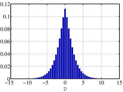
Figure 1: Histogram of decision variable $D$

V Conclusions

In [1] is presented an analysis of complex Gaussian quadratic forms which gives some powerful expressions to study many digital communications systems in terms of the error probability. This analysis has been revised in this technical report, obtaining alternative expressions in a compact matrix format. Little mistakes in the original expressions have been detected which must be corrected to avoid errors in practical applications. Finally, a simple example has been presented which reveals the influence of these mistakes and confirms the validity of the new expressions.

References

- [1] J. G. Proakis, “On the probability of error for multichannel reception of binary signals” IEEE Trans. Commun. Technol., vol. 16, pp. 68-71, Feb 1968.
- [2] J. G. Proakis, Digital Communications, 4th ed., New York, Mc Graw-Hill, 2001.
- [3] M.K. Simon, M. Alouini, Digital Communication over Fading channels, 2nd ed., New Jersey, John Wiley & Sons, 2005.
- [4] M.K. Simon, M. Alouini, “A Unified Approach to the Performance Analysis of Digital Communication over Generalized Fading Channels” in Proc. IEEE, vol. 86, no. 9, pp. 1860-1877, Sep. 1998
- [5] S. Gaur, A. Annamalai, “Some Integrals Involving the With Application to Error Probability Analysis of Diversity Receivers” IEEE Trans. on Vehicular Technology, vol. 52, no. 6, pp. 1568-1575, Nov 2003.
- [6] L. Cao, C. Beaulieu,“Closed-Form BER Results for MRC Diversity With Channel Estimation Errors in Ricean Fading Channels” IEEE Trans. on Wireless Communications, vol. 4, no. 4, pp. 1440-1447, July 2005.
- [7] J. Lu, T. T. Tjhung, F. Adachi, C.L. Huang, “BER Performance of OFDM-MDPSK System in Frequency-Selective Rician Fading with Diversity Reception” IEEE Trans. on Vehicular Technology, vol. 49, no. 4, pp. 1216-1225, Jul. 2000.
- [8] M.L. McCloud, M.K. Varanasi, “Modulation and Coding for Noncoherent Communications” Journal of VLSI Signal Processing, no. 30, pp. 35-54, 2002.
- [9] K. H. Biyari, W.C. Lindsey, “Statistical Distribution of Hermitian Quadratic Forms in Complex Gaussian Variables” IEEE Trans. on Information Theory, vol. 39, no. 3, pp. 1076-1082, May 1993.
- [10] G.L. Turin, “The characteristic function of Hermitian quadratic forms in complex normal variables” Biometrika, vol. 47, no. 1-2, pp. 199–201, 1960.
- [11] W.C. Lindsey, “Error Probabilities for Rician Fading Multichannel Reception of Binary and N-ary Signals” IEEE Trans. on Information Theory, vol. IT-10, pp. 339-350,Oct. 1964.