Joint Assessment of the Differential Item Functioning
and Latent Trait Dimensionality
of Students’ National Tests

Abstract

Within the educational context, students’ assessment tests are routinely validated through Item Response Theory (IRT) models which assume unidimensionality and absence of Differential Item Functioning (DIF). In this paper, we investigate if such assumptions hold for two national tests administered in Italy to middle school students in June 2009: the Italian Test and the Mathematics Test. To this aim, we rely on an extended class of multidimensional latent class IRT models characterised by: (i) a two-parameter logistic parameterisation for the conditional probability of a correct response, (ii) latent traits represented through a random vector with a discrete distribution, and (iii) the inclusion of (uniform) DIF to account for students’ gender and geographical area. A classification of the items into unidimensional groups is also proposed and represented by a dendrogram, which is obtained from a hierarchical clustering algorithm. The results provide evidence for DIF effects for both Tests. Besides, the assumption of unidimensionality is strongly rejected for the Italian Test, whereas it is reasonable for the Mathematics Test.

Keywords: EM algorithm; Hierarchical clustering; Item Response Theory; Multidimensional latent variable models; Two-parameter logistic parameterisation.

1 Introduction

Italian National Tests for the assessment of primary, lower middle, and high-school students are developed and yearly collected by the National Institute for the Evaluation of the Education System (INVALSI). Before administration, national tests are validated through pretesting sessions. These preliminary data are analysed by standard Classical Test and Item Response Theory (IRT) models (Hambleton and Swaminathan,, 1985).

In this paper, we focus on the Tests administered to middle school students as they are having an increasing relevance in the Italian education context and their collection will become compulsory in the near future. In particular, we aim at studying if the assumptions of the IRT models used by the INVALSI to calibrate the national Tests are met for the “live” data collected by this Institution in June 2009, focusing in particular on the assumptions of unidimensionality and of no Differential Item Functioning (DIF). The data are based on a nationally representative sample of 27,592 students within 1,305 schools (one class is sampled in each school) and refer to students’ performances in two national tests, the Italian Test and the Mathematics Test, administered in June 2009.

In accordance with the assumption of unidimensionality, which characterizes the most common IRT models, responses to a set of items only depend on a single latent trait which, in the educational setting, can be interpreted as the student’s ability. However, if unidimensionality is not met, summarizing students’ performances through a single score, on the basis of a unidimensional IRT model, may be misleading as test items indeed measure more than one ability. Absence of DIF means that the items have the same difficulty for all subjects and, therefore, difficulty does not vary among different groups defined, for instance, by gender or geographical area.

In connection with the Rasch model, the hypothesis of unidimensionality has been extensively tested in the literature on the subject (Rasch,, 1961; Glas and Verhelst,, 2007; Verhelst,, 2001). One of the main contributions has been developed by Martin-Löf, (1973), who proposed to test the hypothesis that the Rasch model holds for the whole set of items against the hypothesis that this model holds for two disjoint subsets of items defined in advance. Therefore, most statistical tests proposed in the literature are based on the assumptions that: (i) item discrimination power is constant and (ii) the conditional probability to answer a given item correctly does not vary across different groups. It is plausible that, given the complexity of the INVALSI study, these assumptions are not met for the INVALSI Test items as they may not discriminate equally well among subjects and may exhibit differential item functioning (DIF).

In line with the above issues, we illustrate an extension of the class of multidimensional latent class IRT models developed by Bartolucci, (2007) to include DIF effects. Specifically, we consider the version of these models based on a two-parameter logistic (2PL) parameterisation (Birnbaum,, 1968) for the conditional probability of a correct response. The applied models are of latent class type, as they rely on the assumption that the population under study is made up by a finite number of classes, with subjects in the same class having the same ability level (Lazarsfeld and Henry,, 1968; Formann,, 1995; Lindsay et al.,, 1991). Representing the ability distribution through a discrete latent variable is more flexible than representing it by means of a continuous distribution and is compatible with the assumption of multidimensionality, which means that the adopted questionnaire indeed measures more than one type of ability or dimension (Lazarsfeld and Henry,, 1968; Formann,, 1995; Lindsay et al.,, 1991).

On the basis of the extended class of models described above, we analyse the 2009 INVALSI “live” data. These data are collected by two National Tests, which are developed to assess a number of different abilities, such as the ability to make sense of written texts, the ability to understand expressions and equations, and so on. As already mentioned, these Tests are of particular relevance in the Italian educational system; moreover, their reliability is nowadays deeply discussed. With reference to these data, in particular, we test the hypothesis of unidimensionality and that of absence of DIF. Moreover, we provide a clustering of the items, so that the items in the same group are referred to the same ability. This is obtained by performing a sequence of Wald tests between nested multidimensional IRT models belonging to the proposed class. The results of this clustering procedure may be effectively illustrated by dendrograms.

The remainder of this paper is organized as follows. In the next section we describe the INVALSI data used in our analysis. The statistical methodological approach employed to investigate the structure of the questionnaires is described in Section 3. Firstly, we recall the basics for the model adopted in our study (Bartolucci,, 2007); then we show how it can be extended to take into account DIF effects. Details about the estimation algorithm and the use of these models to test unidimensionaly and absence of DIF are given in Section 4. Finally, in Section 5, we illustrate the main results obtained by applying the proposed approach to the INVALSI dataset and in Section 6 we draw the main conclusions of the study.

2 The 2009 INVALSI Tests

In 2009, the INVALSI Italian Test included two sections, a Reading Comprehension section and a Grammar section. The first section is based on two texts: a narrative type text (where readers engage with imagined events and actions) and an informational text (where readers engage with real settings); see INVALSI, 2009b . The comprehension processes are measured by 30 items, which require students to demonstrate a range of abilities and skills in constructing meaning from the two written texts. Two main types of comprehension processes were considered in developing the items: Lexical Competency, which covers the ability to make sense of worlds in the text and to recognize meaning connections among them, and Textual Competency, which relates to the ability to: (i) retrieve or locate information in the text, (ii) make inferences, connecting two or more ideas or pieces of information and recognizing their relationship, and (iii) interpret and integrate ideas and information, focusing on local or global meanings. The Grammar section is made of 10 items, which measure the ability of understanding the morphological and syntactic structure of sentences within a text.

The INVALSI Mathematics Test consisted of 27 items covering four main content domains: Numbers, Shapes and Figures, Algebra, and Data and Previsions (INVALSI, 2009c, ). The Number content domain consists of understanding (and operation with) whole numbers, fractions and decimals, proportions, and percentage values. The Algebra domain requires students the ability to understand, among others, patterns, expressions and first order equations, and to represent them through words, tables and graphs. Shapes and Figures covers topics such as geometric shapes, measurement, location and movement. It entails the ability to understand coordinate representations, to use spatial visualization skills in order to move between two and three dimensional shapes, draw symmetrical figures, and understand and being able to describe rotations, translations, and reflections in mathematical terms. The Data and Previsions domain includes three main topic areas: data organization and representation (e.g., read, organize and display data using tables and graphs), data interpretation (e.g., identify, calculate and compare characteristics of datasets, including mean, median, mode), and chance (e.g., judge the chance of an outcome, use data to estimate the chances of future outcomes).

All items included in the Italian Test are of multiple choice type, with one correct answer and three distractors, and are dichotomously scored (assigning 1 point to correct answers and 0 otherwise). The Mathematics Test is also made of multiple choice items, but it also contains two open questions for which a partial score of 1 was assigned to partially correct answers and a score of 2 was given to correct answers.

The two Tests were administered in June 2009, at the end of the pupils’ compulsory educational period. Afterwards, a nationally representative sample made of 27,592 students was drawn through a stratified random sampling (INVALSI, 2009a, ). From each of the 21 strata (the 21 Italian geographic regions) a sample of schools was drawn independently and allocation of sample units within each stratum was chosen proportional to an indicator based on the standard deviations of certain variables and the stratum sizes (Neyman,, 1934). Classes within schools were then sampled through a random procedure, with one class sampled in each school, without taking into account the class size (only schools with less than 10 students were excluded from the sampling procedure). Overall, 1305 schools (and classes) were sampled. Table 1 and Table 2 show the distribution of students per gender and geographic areas, respectively for the Italian Test and the Mathematics Test.

Gender	Geographic area
	NW	NE	Centre	South	Islands	Total
Females	1969	2203	2099	2194	2173	10638
Males	1922	2155	2242	2258	2182	10759
Total	3891	4358	4341	4452	4355	21397

Table 1: Distribution of students per gender and geographic area for the INVALSI Italian Test.

Gender	Geographic area
	NW	NE	Centre	South	Islands	Total
Females	1606	1940	1786	1884	1831	8825
Males	1538	1804	1840	1866	1777	9047
Total	3144	3744	3626	3750	3608	17872

Table 2: Distribution of students per gender and geographic area for the INVALSI Mathematics Test.

Preliminary analyses (see Table 3 and Table 4) confirm that students’ performances on Test items were different on account of students’ gender and geographic area. Overall, females performed better than males in the Italian Test, but worse than males in the Mathematics Test. In both Tests, average percentage scores per geographic area revealed very diverse levels of attainment. Generally, students from the Center of Italy performed better than the rest of the students in the Italian Test.

Gender	Geographic area
	NW	NE	Centre	South	Islands	Overall
Females	75.0	73.9	76.2	75.2	73.6	74.8
Males	73.0	71.4	73.1	73.4	71.0	72.4
Overall	74.0	72.6	74.6	74.3	72.3	73.6

Table 3: Average percentage score per gender and geographic area for the INVALSI Italian Test.

Gender	Geographic area
	NW	NE	Centre	South	Islands	Overall
Females	73.3	71.9	75.6	77.5	76.3	75.0
Males	75.6	74.9	76.8	77.8	76.8	76.4
Overall	74.4	73.4	76.2	77.6	76.5	75.7

Table 4: Average percentage score per gender and geographic area for the INVALSI Mathematics Test.

3 Methodological approach

In this section, we illustrate the methodological approach adopted to investigate the presence of DIF and the dimension of the latent structure behind the analysed data. Firstly, we review the basic model proposed by Bartolucci, (2007) and then we extend it to include DIF effects.

3.1 Preliminaries

The multidimensional latent class (LC) IRT models developed by Bartolucci, (2007) presents two main differences with respect to the classic IRT models: (i) the latent structure is multidimensional and (ii) it is based on latent variables that have a discrete distribution. We consider in particular the version of these models based on the two-parameter (2PL) logistic parameterisation of the conditional response probabilities.

Let $n$ denote the number of subjects in the sample and suppose that these subjects answer $r$ dichotomous test items which measure $s$ different latent traits or dimensions. Also let $\mathcal{J}_{d}$, $d=1,\ldots,s$, be the subset of $\mathcal{J}=\{1,\ldots,r\}$ containing the indices of the items measuring the latent trait of type $d$ and let $r_{d}$ denoting the cardinality of this subset, so that $r=\sum_{d=1}^{r}s_{d}$. Since we assume that each item measures only one latent trait, the subsets $\mathcal{J}_{d}$ are disjoint; obviously, these latent traits may be correlated. Moreover, adopting a 2PL parameterisation (Birnbaum,, 1968), it is assumed that

$$\textrm{logit}[p(Y_{ij}=1\mid\mbox{\boldmath$\Theta$}_{i}=\mbox{\boldmath$\theta$})]=\gamma_{j}\left(\sum_{d=1}^{D}\delta_{jd}\theta_{d}-\beta_{j}\right),\quad i=1,\ldots,n,\>j=1,\ldots,r.$$ (1)

In the above expression, $Y_{ij}$ is the random variable corresponding to the response to item $j$ provided by subject $i$ ($Y_{ij}=0,1$ for wrong or right response, respectively). Moreover, $\beta_{j}$ and $\gamma_{j}$ are, respectively, the difficulty and the discrimination of item $j$, $\mbox{\boldmath$\Theta$}_{i}=(\Theta_{i1},\ldots,\Theta_{is})^{\prime}$ is the vector of latent variables corresponding to the different traits measured by the test items, $\mbox{\boldmath$\theta$}=(\theta_{1},\ldots,\theta_{s})^{\prime}$ denotes one of the possible realizations of $\mbox{\boldmath$\Theta$}_{i}$, and $\delta_{jd}$ is a dummy variable equal to $1$ if item $j$ belongs to $\mathcal{J}_{d}$ (and then it measures the $d$th latent trait) and to 0 otherwise. Finally, a crucial assumption is that each random vector $\mbox{\boldmath$\Theta$}_{i}$ has a discrete distribution with support $\{\mbox{\boldmath$\xi$}_{1},\ldots,\mbox{\boldmath$\xi$}_{k}\}$, which correspond to $k$ latent classes in the population. The elements of each vector $\mbox{\boldmath$\xi$}_{c}$ are denoted by $\xi_{cd}$, $d=1,\ldots,s$, with $\xi_{cd}$ denoting the ability level of subjects in latent class $c$ with respect to dimension $d$. Note that, when $\gamma_{j}=1$ for all $j$, then the above 2PL parameterisation reduces to a multidimensional Rasch parameterisation (Rasch,, 1961). At the same time, when the elements of each support vector $\mbox{\boldmath$\xi$}_{c}$ are obtained by the same linear transformation of the first element, the model is indeed unidimensional even when $s>1$. The last consideration will be useful in order to compute $p$-values for the test of unidimensionality.

As for the conventional LC model (Lazarsfeld and Henry,, 1968; Goodman,, 1974), the assumption that the latent variables have a discrete distribution implies the following manifest distribution of the full response vector $\mbox{\boldmath$Y$}_{i}=(Y_{i1},\ldots,Y_{ir})^{\prime}$:

$$p_{i}(\mbox{\boldmath$y$})=p(\mbox{\boldmath$Y$}_{i}=\mbox{\boldmath$y$})=\sum_{c=1}^{k}p_{i}(\mbox{\boldmath$y$}\mid c)\pi_{c},$$ (2)

where $\mbox{\boldmath$y$}=(y_{1},\ldots,y_{r})^{\prime}$ denotes a realisation of $\mbox{\boldmath$Y$}_{i}$, $\pi_{c}=p(\mbox{\boldmath$\Theta$}_{i}=\mbox{\boldmath$\xi$}_{c})$ is the weight of the $c$th latent class, and

$$p_{i}(\mbox{\boldmath$y$}\mid c)=p(\mbox{\boldmath$Y$}_{i}=\mbox{\boldmath$y$}\mid\mbox{\boldmath$\Theta$}_{i}=\mbox{\boldmath$\xi$}_{c})=\prod_{j=1}^{r}p(Y_{ij}=y_{j}\mid\mbox{\boldmath$\Theta$}_{i}=\mbox{\boldmath$\xi$}_{c}),\quad c=1,\ldots,k.$$ (3)

The specification of the multidimensional LC 2PL model, based on the assumptions illustrated above, univocally depends on: (i) the number of latent classes ($k$), (ii) the number of the dimensions ($s$), and (iii) the way items are associated to the different dimensions. The last feature is related to the definition of the subsets $\mathcal{J}_{d}$, $d=1,\ldots,s$.

3.2 Extension for Differential Item Functioning

DIF occurs when subjects belonging to different groups (commonly defined by gender, ethnicity, or geographic area) with the same latent trait level have a different probability of providing a certain answer to a given item (Thissen et al.,, 1993; Clauser and Mazor,, 1998; Swaminathan and Rogers,, 1990).

Even in the presence of a 2PL parameterisation, it reasonable to suppose that the main reason of DIF is due to the item difficulty level, which may depend on the individual characteristics of the respondent. More precisely, the presence of DIF in the difficulty level of item $j$ may be represented by shifted values of $\beta_{j}$ for one group of subjects with respect to another.

Let $z_{gi}$ be a dummy variable which assumes value 1 if subject $i$ belongs to group $g$ (e.g., that of females) and value 0 otherwise. The number of groups is denoted by $h$, so that, in the previous expression, $g=1,\ldots,h$. When $s=1$, the 2PL parameterisation may be extended for DIF by assuming:

$$\mbox{logit }[p(Y_{ij}=1\mid\Theta_{i}=\theta)]=\gamma_{j}\left[\theta-\left(\beta_{j}+\sum_{g=1}^{h}\phi_{gj}z_{gi}\right)\right],\quad i=1,\ldots,n,\>j=1,\ldots,k,$$ (4)

where $\phi_{gj}$ measures the shift for item $j$ in terms of difficulty. Therefore, if two subjects have the same ability level $\theta$, but belong to two different groups, say $g_{1}$ and $g_{2}$, the difference between the corresponding conditional probabilities of a correct response is $\phi_{g_{1}j}-\phi_{g_{2}j}$ on the logit scale. It can be observed that this difference between logits does not depend on the common latent trait value $\theta$. In this case, the so-called uniform DIF arises; see Thissen et al., (1993), Clauser and Mazor, (1998), and Swaminathan and Rogers, (1990).

Obviously, DIF in the difficulty level may be also introduced in the multidimensional case and when subjects are classified according to more criteria, to give an additive structure to the corresponding DIF effects. More precisely, suppose that, as in our applications, subjects are grouped according to two criteria and that the first criterion gives rise to $h_{1}$ groups, whereas the second gives rise to $h_{2}$ groups. Then, as an extension of (1), we have

$$\textrm{logit}[p(Y_{ij}=1\mid\mbox{\boldmath$\Theta$}_{i}=\mbox{\boldmath$\theta$})]=\gamma_{j}\left[\sum_{d=1}^{s}\delta_{jd}\theta_{d}-\left(\beta_{j}+\sum_{g=1}^{h_{1}}\phi_{gj}^{(1)}z_{hi}^{(1)}+\sum_{g=1}^{h_{2}}\phi_{gj}^{(2)}z_{hi}^{(2)}\right)\right],$$ (5)

for $i=1,\ldots,n$ and $j=1,\ldots,r$. In the above expression, each dummy variable $z_{gi}^{(1)}$ is equal to 1 if subject $i$ belongs to group $g$ (when the classification of subjects is based on the first criterion) and to 0 otherwise; $\phi_{gj}^{(1)}$ is the corresponding DIF parameter. The dummy variables $z_{gi}^{(2)}$ and the parameters $\phi_{gj}^{(2)}$ are defined accordingly. These parameters may be simply interpreted as clarified above.

In the approach proposed in this paper, we rely on assumption (5) to extend the class of model of Bartolucci, (2007) for DIF, even under the 2PL parameterisation and in the presence of multidimensionality.

4 Likelihood based inference

In this section, we deal with the maximum likelihood of the extended model based on assumption (5) and with the problem of selecting the number of latent states, and testing hypotheses on the parameter. The hypotheses of greatest interest in our context are those of absence of DIF and unimensionality. We also briefly outline the algorithm for clustering items in unidimensional groups.

4.1 Maximum likelihood estimation

Let $\mbox{\boldmath$y$}_{i}$, $i=1,\ldots,n$, denote the response configuration provided by subject $i$. For a given $k$, the parameters of the proposed model may be estimated by maximizing the log-likelihood

$$\ell(\mbox{\boldmath$\eta$})=\sum_{i}\log[p_{i}(\mbox{\boldmath$y$}_{i})],$$ (6)

where $\eta$ is the vector containing all the free parameters, and $p_{i}(\mbox{\boldmath$y$})$ is the manifest mass probability function of $y$ defined in (2) on the basis of the model parameters. When subjects are classified according to only one criterion, an equivalent expression for the log-likelihood is the following

$$\ell(\mbox{\boldmath$\eta$})=\sum_{g=1}^{h}\sum_{\mbox{\footnotesize\boldmath{$y$}}}n(g,\mbox{\boldmath$y$})\log[p_{g}^{*}(\mbox{\boldmath$y$})],$$ (7)

where $n(g,\mbox{\boldmath$y$})$ is the frequency, in the sample, of subjects who belong to group $g$ and provide response configuration $y$, and $p_{g}^{*}(\mbox{\boldmath$y$})$ is the manifest probability of $y$ for the subjects. Moreover, the sum $\sum_{\mbox{\footnotesize\boldmath{$y$}}}$ is extended to all response configurations observed at least once. Similar expressions result when subjects are classified according to more criteria.

About the vector $\eta$, we clarify that it contains the item parameters $\beta_{j}$ (difficulty) and $\gamma_{j}$ (discriminating index), and $\phi_{gj}$ (DIF parameters), the parameters $\xi_{cd}$ (ability levels) and $\pi_{c}$ (corresponding weights). However, to make the model identifiable, we adopt the constraints

$$\beta_{j_{d}}=0,\>\gamma_{j_{d}}=1,\quad d=1,\ldots,s,$$

with $j_{d}$ denoting a reference item for the $d$-th dimension (usually, but not necessarily, the first one in the group). When subjects are classified according to only one criterion, we have

$$\phi_{1j}=0,\quad j=1,\ldots,r,$$ (8)

where the first group is taken as reference group. In this way, for each item $j$, with $j\in(\mbox{${\cal J}$}_{d}\setminus\{j_{d}\})$, the parameter $\beta_{j}$ is interpreted in terms of differential difficulty level of this item with respect to item $j_{d}$; similarly, $\gamma_{j}$, is interpreted in terms of ratio between the discriminant index of item $j$ and that of item $j_{d}$. Finally, for $g>1$, $\phi_{gj}$ corresponds to the differential difficultly level of group $g$, with respect to the first group, for item $j$. When subjects are classified according to, say, two criteria and assumption (5) is adopted, then the identifiability constraints

$$\phi^{(1)}_{1j}=\phi^{(2)}_{1j}=0,\quad j=1,\ldots,r,$$

must be used instead in (8).

Considering the above identifiability constraints, when $k>2$ and subjects are classified according to a single criterion with regard to DIF, the number of free parameters collected in $\eta$ is equal to

$$\#{\rm par}=(k-1)+ks+2(r-s)+r(h-1),$$

since there are $k-1$ free latent class probabilities, $ks$ free ability parameters $\xi_{cd}$, $r-s$ free difficulty parameters and discriminant indices, and $r(h-1)$ free DIF parameters. For $k=1,2$, the proposed model does not pose any restriction over the LC model and then we have $\#{\rm par}=(k-1)+kr+r(h-1)$. The number of parameters is simply modified when subjects are classified according to more criteria. For instance, when the classification is based on two criteria, and then assumption (5) holds, the term $r(h-1)$ in $\#{\rm par}$ need to be substituted by $r(h_{1}+h_{2}-2)$.

In order to maximise the log-likelihood $\ell(\mbox{\boldmath$\eta$})$, we make use of the Expectation-Maximization (EM) algorithm (Dempster et al.,, 1977), which is implemented along the same lines as in Bartolucci, (2007). This algorithm is briefly described in Appendix 1; a Matlab implementation is available from the authors upon request. The maximum likelihood estimate of $\eta$, obtained from maximisation of $\ell(\mbox{\boldmath$\eta$})$, is denoted by $\hat{\mbox{\boldmath$\eta$}}$.

After the parameter estimation, each subject $i$ can be allocated to one of the $k$ latent classes on the basis of the response pattern $\mbox{\boldmath$y$}_{i}$ he/she provided. The most common approach is to assign the subject to the class with the highest posterior probability. On the basis of the parameter estimates, the posterior probability is computed as

$$\hat{q}_{i}(c\mid\mbox{\boldmath$y$}_{i})=\hat{p}_{i}(\mbox{\boldmath$\Theta$}_{i}=\mbox{\boldmath$\xi$}_{c}\mid\mbox{\boldmath$Y$}_{i}=\mbox{\boldmath$y$}_{i})=\frac{\hat{p}_{i}(\mbox{\boldmath$y$}_{i}|\mbox{\boldmath$\xi$}_{c})\hat{\pi}_{c}}{\sum_{h=1}^{k}\hat{p}_{i}(\mbox{\boldmath$y$}_{i}|\mbox{\boldmath$\xi$}_{h})\hat{\pi}_{h}},\quad c=1,\ldots,C.$$ (9)

4.2 Choice of the number of latent classes, hypothesis testing, and dimensionality assessment

In analysing a dataset by the model described in Section 3, a crucial point is the choice of the number of latent classes $k$. To this aim, we rely on the Bayesian Information Criterion (BIC) of Schwarz, (1978). On the basis of this criterion, the selected number of classes is the one corresponding to the minimum value of

$$BIC=-2\ell(\hat{\mbox{\boldmath$\eta$}})+\log(n)\#{\rm par}.$$

In practice, we fit the model for increasing values of $k$ until $BIC$ does not start to increase and then we take the previous value of $k$ as the optimal one.

Once the number of latent states has been selected, it is of interest to test several hypotheses on the parameters. To this aim, we can follow the general likelihood ratio (LR) approach. For a hypothesis of type $H_{0}:\mbox{\boldmath$f$}(\mbox{\boldmath$\eta$})=\mbox{\boldmath$0$}$, where $\mathrm{𝟎}$ denotes a column vector of zeros of suitable dimension, this approach is based on the statistic

$$D=-2[\ell(\hat{\mbox{\boldmath$\eta$}}_{0})-\ell(\hat{\mbox{\boldmath$\eta$}})],$$ (10)

which, under the usual regularity conditions, has null asymptotic distribution of $\chi^{2}_{m}$ type, where $m$ is the number of constraints imposed by $H_{0}$. An alternative approach is based on the Wald test which is based on the statistic

$$W=\mbox{\boldmath$f$}(\hat{\mbox{\boldmath$\eta$}})^{\prime}\mbox{\boldmath$G$}(\hat{\mbox{\boldmath$\eta$}})\mbox{\boldmath$f$}(\hat{\mbox{\boldmath$\eta$}}),$$ (11)

where $\mbox{\boldmath$G$}(\mbox{\boldmath$\eta$})$ is a suitable matrix computed on the basis of the Jacobian of $\mbox{\boldmath$f$}(\mbox{\boldmath$\eta$})$ and the information matrix of the model. It is well known that the two approaches are asymptotically equivalent, and that, differently from the LR approach, the one based on the statistic $W$ only requires to fit the larger model, but also to compute the information matrix of the model, which may be rather complex.

On the basis of the above approach, we can test the hypothesis of absence of DIF. In this case, the null hypothesis is

$$H_{0}:\phi_{gj}=0,\quad g=2,\ldots,h,\>j=1,\ldots,r,$$

or

$$H_{0}:\phi_{2j}^{(1)}=\cdots=\phi_{h_{1}j}^{(1)}=\phi^{(2)}_{2j}=\cdots=\phi^{(2)}_{h_{2}j}=0,\quad j=1,\ldots,r,$$ (12)

when subjects are classified according to two criteria for what concerns DIF. Then, to test $H_{0}$, we have to fit the model with and without DIF and compare the corresponding log-likelihoods by (10). Thus, if the obtained value of test statistic is higher than a suitable percentile of the $\chi^{2}_{m}$ distribution, with $m=r(h-1)$, we reject $H_{0}$ and can state that there is evidence of DIF.

The above approach may also be used for the hypothesis that a group of items measure only one latent trait, that is unidimensionality, against the hypothesis that the same group is multidimensional. In the case of two dimensions, for instance, we have to compare by the LR statistic (10) the model in which these dimensions are kept distinct with the model in which these dimensions are collapsed. Under the null hypothesis of unidimensionality, this test statistic has an asymptotic distribution of $\chi^{2}_{m}$ type, with $m=k-2$. This is because, as mentioned in Section 3.1, unidimensionality holds when the ability level for the second dimension may be obtained by the same linear transformation of the ability level for the first dimension, for every latent class $c$. Obviously, this test makes only sense when $k>2$ and, in general, may also be performed by a Wald statistic of type (11), once the function $\mbox{\boldmath$f$}(\mbox{\boldmath$\eta$})$ has been suitably defined; see Bartolucci, (2007) for details.

By repeating the test for unimensionality mentioned above in a suitable way, we can cluster items so that items in the same group measure the same ability. On the basis of this principle, Bartolucci, (2007) proposed a hierarchical clustering algorithm that we also apply for the extended models here proposed, which account for DIF. This algorithm builds a sequence of nested models: the most general one is that with a different dimension for each item (corresponding to the classic LC model in absence of DIF) and the most restrictive model is that with only one dimension common to all items (unidimensional model). The clustering procedure performs $s-1$ steps. At each step, the Wald test statistic for unidimensionality is computed for every pair of possible aggregations of items (or groups of items). The aggregation with the minimum value of the statistic (or equivalently the highest $p$-value) is then adopted and the corresponding model fitted before going to the next step. A similar strategy could be based on the LR statistic, but in this case we would be required to fit a much higher number of models. A Matlab implementation of this algorithm is also available from the authors upon request.

The output of the above clustering algorithm may be displayed through a dendrogram that shows the deviance between the initial ($k$-dimensional) LC model and the model selected at each step of the clustering procedure. Obviously, the results of a cluster analysis based on a hierarchical procedure depend on the adopted rule to cut the dendrogram, which may be chosen according to several criteria. A rule that may be adopted to cut the dendrogram is based on the increase of a suitable information criterion, such as BIC, with respect to the initial or the previous fitted model. A negative increase of BIC means that the new model reaches a better compromise between goodness-of-fit and parsimony than the model used as a comparison term (i.e., the initial or the previous one). The dendrogram is cut when the item aggregation does not give any additional advantages, that is, in correspondence with the last step showing a negative increase.

5 Application to the INVALSI dataset

In this section, we apply the extended class of models to the data collected by the two INVALSI Tests. For the purposes of the analysis, the 30 items which assess reading comprehension within the Italian Test are kept distinct from the 10 items which assess grammar competency, as the two sections deal with two different competencies. Besides, since we do not have any prior information on item discrimination power, we choose the 2PL parameterisation and, regarding the way of taking DIF effects into account, we consider subjects classified according to gender ($h_{1}=2$ categories: Males, Female) and geographical area ($h_{2}=5$ categories: NorthWest, NorthEast, Centre, South, Islands). Then, the adopted parameterisation is the same as in (5). The categories Males and NorthWest are taken as reference categories.

In the following, we deal with the selection of the number of latent classes, with the problem of testing the hypothesis of absence of DIF, and with the issue of clustering items.

5.1 Selection of the number of classes

In order to choose the number of latent classes we proceed as described in Section 4.2 and fit the model in the multidimensional version, in which each item is assumed to measure a single ability, for values of $k$ from 1 to 9. The maximum value of $k$ is chosen to be equal to 9 as it is the first value for which $BIC$ is higher than that associated to the previous value of $k$ for all Test sections. The results of this preliminary fitting are reported in Table 5.

$k$	Reading comprehension			Grammar			Mathematics
	$\ell(\hat{\mbox{\boldmath$\eta$}})$	$\#{\rm par}$	$BIC$	$\ell(\hat{\mbox{\boldmath$\eta$}})$	$\#{\rm par}$	$BIC$	$\ell(\hat{\mbox{\boldmath$\eta$}})$	$\#{\rm par}$	$BIC$
1	-350,474	180	702,743	-100,842	60	202,282	-242,111	162	485,808
2	-329,109	211	660,323	-95,580	71	192,899	-224,506	190	450,873
3	-326,171	242	654,760	-95,645	82	192,110	-221,976	218	446,090
4	-325,516	273	653,750	-95,580	93	192,090	-220,936	246	444,280
5	-324,970	304	652,970	-95,517	104	192,070	-220,032	274	442,750
6	-324,863	335	653,070	-95,470	115	192,090	-219,619	302	442,190
7	-324,764	366	653,178	-95,464	126	192,184	-219,248	330	441,730
8	-324,684	397	653,327	-95,454	137	192,274	-218,977	358	441,460
9	-324,583	428	653,436	-95,429	148	192,334	-218,846	386	441,470

Table 5: Log-likelihood, number of parameters and BIC values for $k=1,\ldots,9$ latent classes for the Reading Comprehension and the Grammar sections of the Italian Test and for the Mathematics Test; in boldface is the smallest BIC value for each type of Test.

On the basis of BIC, we choose $k=5$ classes both for the Reading Comprehension and the Grammar sections of the Italian Test. As regards to Mathematics Test, despite $k=8$ being the optimal number of classes, we choose $k=3$, as for each number of classes greater than 3 the model becomes almost nonidentifiable, in the sense that the corresponding information matrix is close to be singular. We recall that this matrix is crucial for performing the Wald test for unidimensionality.

5.2 Testing absence of DIF

As previously specified, we define two groups of students on the basis of gender and geographic area. The null hypothesis of no (uniform) DIF is formulated as in (12). At this regard, Table 6 shows the LR statistic, computed as in (10), between the 2PL multidimensional model with uniform DIF based on assumption (5) and the 2PL multidimensional model based on assumption (1).

	Deviance	$p$-value
Reading Compr.	1579.702	$<$0.001
Grammar	1313.427	$<$0.001
Mathematics	2183.573	$<$0.001

Table 6: Deviance of the multidimensional 2PL model with uniform DIF with respect to the multidimensional 2PL model with no DIF for the Italian Test - Reading Comprehension section and Grammar section - and the Mathematics Test.

According to these results, the assumption of no DIF is strongly rejected for both sections of the Italian Test and for the Mathematics Test. Therefore, in Table 7, Table 8, and Table 9 we provide the estimates of the DIF coefficients ($\phi_{gj}^{(1)}$ and $\phi_{gj}^{(2)}$). We recall that each of these coefficients represents the difference, in terms of difficulty of an item, between one group of subjects with respect to the reference group, given the same ability level.

Item	Females	NorthEast	Centre	South	Islands
R1	-0.018	-0.051	-0.262∗∗∗	-0.173∗∗	0.032
R2	-0.322∗∗∗	0.132	-0.005	-0.073	0.170
R3	0.021	0.211∗	-0.057	0.212∗	0.131
R4	-0.447∗∗∗	0.253∗	0.291∗∗	0.428∗∗∗	0.613∗∗∗
R5	-0.377∗∗∗	0.192∗	0.094	0.110	0.227∗∗
R6	0.117∗∗	0.132	0.153∗	0.305∗∗∗	0.457∗∗∗
R7	-0.332∗∗∗	0.083	0.040	0.196∗∗	0.433∗∗∗
R8	-0.072∗	0.002	0.127∗	0.229∗∗∗	0.159∗∗
R9	-0.170∗∗∗	0.046	0.008	0.078	0.141∗∗
R10	-0.340∗∗∗	0.320∗	-0.291∗	-0.420∗∗	-0.581∗∗∗
R11	-0.159∗∗∗	0.038	0.075	0.279∗∗∗	0.415∗∗∗
R12	-0.148∗∗∗	0.069	-0.038	0.277∗∗∗	0.227∗∗∗
R13	-0.057∗	0.003	0.003	-0.035	0.111∗
R14	0.096	0.019	-0.060	0.176∗	0.159∗
R15	0.001	-0.026	-0.079	-0.079	0.028
R16	-0.352∗∗∗	0.270∗∗	-0.387∗∗∗	-0.682∗∗∗	-0.661∗∗∗
R17	-0.074∗∗	0.058	-0.065	-0.017	0.067
R18	0.109∗∗	0.036	0.075	0.232∗∗∗	0.350∗∗
R19	0.260∗∗	0.044	-0.075	-0.480∗∗∗	-0.566∗∗∗
R20	0.029	0.049	0.283∗∗∗	0.207∗∗	0.236∗∗
R21	-0.195∗∗∗	-0.068	0.018	0.327∗∗∗	0.290∗∗
R22	-0.193∗∗∗	0.020	-0.022	0.216∗∗∗	0.334∗∗∗
R23	-0.254∗∗∗	0.050	0.025	0.431∗∗∗	0.441∗∗∗
R24	-0.245∗	0.223	-0.282∗	-0.216	-0.067
R25	-0.068	-0.043	0.001	-0.173∗	-0.056
R26	-0.319∗∗∗	0.053	-0.106	-0.158∗∗	0.160∗∗
R27	-0.239∗∗∗	-0.116	-0.079	0.150	0.313∗∗∗
R28	-0.286∗∗∗	0.094	-0.105	-0.215∗∗	-0.014
R29	-0.179∗∗∗	-0.071	-0.117	0.008	0.252 ∗∗
R30	-0.405∗∗∗	0.026	-0.119	0.182∗	0.309∗∗∗

Table 7: Estimated DIF coefficients for the Italian Test items - Reading Comprehension Section; significance at levels 0.001 (***), 0.01 (**), 0.05 (*).

The results in the previous tables show that the Italian Test generally favours girls; conversely, the items of the Mathematics Test tend to favour boys. When taking into account students’ geographic area, we observe that the incidence of items affected by DIF is, on the whole, stronger for the southern regions (Islands included) than the central and northeastern regions, with a higher proportion of items significantly affected by DIF when accounting for the former geographic areas, both in the Italian Test and in the Mathematics Test. Specifically, as for the two sections of the Italian Test, the analysis shows that students from the southern regions tend to have a lower chance to answer the items correctly than students from the other Italian regions. On the contrary, Mathematics Test items generally tend to favour students from the South of Italy.

5.3 Dimensionality assessment

Once the model which includes DIF has been adopted, with a specific $k$ for each Test section (as defined in Section 5.1), we performed the item clustering algorithm described in Section 4.2. The output of this algorithm is represented by the dendrograms in Figures 1, 2, and 3, which are referred, respectively, to the Reading Comprehension section of the Italian Test, to the Grammar section of the same Test, and to the Mathematics Test.

Item	Females	NorthEast	Centre	South	Islands
G1	-0.404∗∗∗	0.133	0.073	0.129	0.428∗∗∗
G2	-0.272∗∗∗	0.156∗	0.060	0.051	0.114
G3	-0.137∗∗∗	0.059	-0.191∗∗	-0.198∗∗	-0.002
G4	-0.052	0.323∗∗∗	0.004	-0.679∗∗∗	-0.350∗∗∗
G5	-0.328∗∗∗	0.118∗	-0.111∗	-0.141∗∗	0.126∗
G6	-0.261∗∗∗	0.362∗∗∗	-0.043	-0.312∗∗∗	0.072
G7	-0.323∗∗∗	0.197∗∗∗	-0.131∗	-0.287∗∗∗	-0.011
G8	-0.309∗∗∗	0.060	0.144	0.099	0.524∗∗∗
G9	-0.205∗	-0.084	-0.067	0.290∗	0.705∗∗∗
G10	-0.167∗	0.269∗	-0.280∗	-0.504∗∗∗	-0.324∗

Table 8: Estimated DIF coefficients for the Italian Test items - Grammar Section; significance at levels 0.001 (***), 0.01 (**), 0.05 (*).

Item	Females	NorthEast	Centre	South	Islands
M1	0.092	0.013	-0.193∗∗	-0.426∗∗∗	-0.423∗∗∗
M2	-0.027	0.058	-0.051	-0.050	0.045
M3	0.023	0.058	-0.044	-0.277∗∗∗	-0.200∗∗∗
M4	0.008	0.076∗	-0.021	-0.030	0.006
M5	0.024	0.102	0.109	0.057	-0.060
M6	-0.002	0.012	-0.102	0.072	0.076
M7	0.036	-0.097	0.073	-0.090	-0.139∗∗∗
M8	0.022	-0.058	0.001	0.144	0.148
M9	0.071∗∗∗	-0.022	-0.056∗	-0.078∗∗	-0.027
M10	0.102∗∗∗	0.023	-0.041	-0.083∗∗	-0.077∗∗
M11	0.029∗	0.031	-0.120∗∗∗	-0.310∗∗∗	-0.310∗∗∗
M12	0.087∗∗∗	0.024	-0.057∗	-0.072	0.022
M13	0.055∗∗∗	0.101∗∗∗	-0.027	-0.073∗∗	-0.024
M14	0.052∗∗	0.065∗∗	-0.031	-0.166∗∗∗	-0.193∗∗∗
M15	0.052∗∗	0.037	-0.012	0.047	-0.002
M16	0.161∗∗∗	0.030	0.019	-0.008	-0.019
M17	0.164∗∗∗	-0.001	-0.056	-0.060	0.018
M18	0.049∗∗∗	-0.001	-0.023	-0.022	-0.025
M19	-0.008	-0.006	0.032	0.103∗∗∗	0.183∗∗∗
M20	-0.024	0.029	-0.007	-0.055∗	-0.006
M21	0.112∗∗∗	0.104∗∗	0.023	-0.034	-0.022
M22	0.033	0.078∗	-0.036	0.001	-0.060∗
M23	0.013	0.049∗	-0.049∗	-0.062∗∗	-0.057∗∗
M24	-0.012	-0.008	-0.097∗∗∗	-0.143∗∗∗	-0.125∗∗∗
M25	-0.035∗∗	-0.013	0.033	0.032	0.153∗∗∗
M26	0.087∗∗∗	0.089∗∗	-0.058	-0.163∗∗∗	-0.083∗
M27	0.010	0.093∗∗	-0.074	-0.269∗∗∗	-0.312∗∗∗

Table 9: Estimated DIF coefficients for the Mathematics Test items; significance at levels 0.001 (***), 0.01 (**), 0.05 (*).

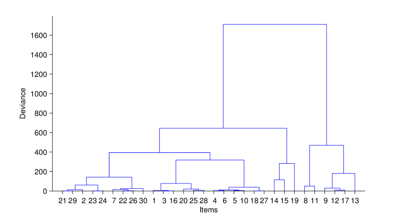
Figure 1: Dendrogram for the Italian Test - Reading Comprehension Section

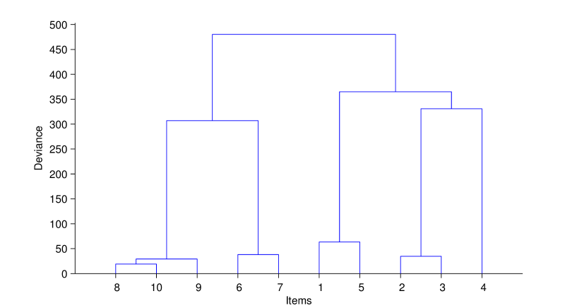
Figure 2: Dendrogram for the Italian Test - Grammar Section

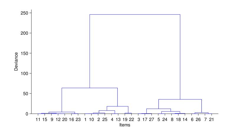
Figure 3: Dendrogram for the Mathematics Test

Following what outlined in Section 3.3, we adopt as a criterion to cut the dendrogram the one based on BIC. In particular, since BIC tends to select more parsimonious models than other criteria (in particular with large sample sizes), and for consistency with the criterion applied to select the number of latent classes, we rely on the increase of BIC with respect to the initial model (i.e., the model with one dimension for each item). The values of the increase of BIC with respect to the initial model are shown in Table 10; note that the number of steps of the clustering algorithm depends on the number of items which are analysed.

The results in Table 10 show that, with the adopted cut criterion and the chosen number of latent classes, the assumption of unidimensionality is not reasonable for both sections of the Italian Test, and in particular for the Grammar section, whereas it is reasonable for the Mathematics Test. Indeed, there is evidence of $s=2$ groups of items in the Reading Comprehension Section of the Italian Test, $s=5$ groups of items in the Grammar Section of the Italian Test, and $s=1$ group of items in the Mathematics Test. The 2 groups observed within the Reading Comprehension Section of the Italian Test are made of 24 and 6 items, corresponding to different, although correlated, dimensions which may be identified as the ability to: (i) make sense of worlds and sentences in the text and recognize meaning connections among them (24 items) and (ii) interpret, integrate and make inferences from a written text (6 items). As regards to the Grammar Section of the Italian Test, the 5 groups of items correspond to the ability to: (i) recognize verb forms (1 item), (ii) recognize the meaning of connectives within a sentence (3 items), (iii) recognize grammatical categories (2 items), (iv) make a difference between clauses within a sentence (2 items), and (v) recognize the meaning of punctuation marks (2 items).

$h$	$s$	Increase BIC with respect to initial model
		Reading compr.	Grammar	Mathematics
1	29	-29.8	-10.755	-9.791
2	28	-59.6	-30.642	-19.581
3	27	-89.0	-55.184	-29.371
4	26	-118.4	-81.534	-39.158
5	25	-147.4	-86.135	-48.942
6	24	-176.4	127.498	-58.723
7	23	-205.4	121.555	-68.499
8	22	-234.0	125.539	-78.275
9	21	-262.6	210.922	-88.043
10	20	-291.0	–	-97.805
11	19	-319.1	–	-107.550
12	18	-346.7	–	-117.241
13	17	-374.0	–	-126.792
14	16	-399.4	–	-136.315
15	15	-424.5	–	-145.827
16	14	-449.3	–	-155.235
17	13	-470.0	–	-164.625
18	12	-488.7	–	-173.480
19	11	-507.3	–	-181.965
20	10	-522.0	–	-190.288
21	9	-514.0	–	-197.723
22	8	-516.5	–	-203.161
23	7	-508.3	–	-206.950
24	6	-435.6	–	-199.422
25	5	-430.4	–	-181.022
26	4	-384.1	–	-8.600
27	3	-339.4	–	–
28	2	-193.6	–	–
29	1	843.4	–	–

Table 10: Diagnostics for the hierarchical clustering algorithm for the Italian Test - Reading Comprehension section and Grammar section - and the Mathematics Test: step of the procedure ($h$), number of groups ($s$), increase of BIC index with respect to the initial model; in boldface are the first positive values.

From Table 11, which shows the support point estimates for the two sections of the Italian Test and the Mathematics Test, it can be also shown that, overall, students’ belonging to the higher latent classes is linked with increasing ability levels.

	$c$
	1	2	3	4	5
Reading Comprehension
Dimension 1	-1.193	0.221	-0.329	1.012	2.776
Dimension 2	-1.404	-0.859	-0.049	0.646	1.378
Grammar
Dimension 1	-0.334	2.244	2.536	2.948	4.363
Dimension 2	-0.853	-0.786	0.812	0.935	2.807
Dimension 3	-0.827	-0.554	-2.068	0.598	2.384
Dimension 4	0.782	1.224	2.012	2.507	3.735
Dimension 5	-0.616	-1.069	-0.623	-0.056	1.364
Mathematics
Dimension 1	0.995	1.509	2.060	–	–

Table 11: Support points estimates for the Italian Test - Reading Comprehension section and Grammar section - and the Mathematics Test

Indeed, students belonging to class 5 within the two sections of the Italian Test, and to class 3 within the Mathematics Test, tend to have the highest ability level in relation with the involved dimensions, whereas students’ belonging to the first latent class is generally associated with lower ability levels. These considerations hold for each dimension but for the first dimension of the Reading Comprehension Section and the third dimension of the Grammar Section - where higher than expected ability levels are observed in correspondence with middle latent classes - and for the fifth dimension of the Grammar Section - where the support point estimate observed by the first latent class is not the lowest.

6 Conclusions

The main objective of this paper is to evaluate the dimensionality of two national Tests employed to assess middle school Italian students’ performance, testing for the assumption of unidimensionality which characterizes most Item Response Theory models used to validate assessment data. We also test if the assumption of absence of Differential Item Functioning (DIF) is reasonable for these data. The data were collected in 2009 by the National Institute for the Evaluation of the Education System (INVALSI) and refer to two assessment Tests - on Italian language competencies (Reading comprehension, Grammar) and Mathematical competencies - administered to middle-school students.

We base our analysis on a class of multidimensional latent class IRT models which allows us to test unidimensionality by concurrently taking into account the presence of DIF and that the items may have non-constant item discrimination power. This class of models is obtained as an extension for (uniform) DIF of the class of multidimensional two-parameter logistic (2PL) models developed by Bartolucci, (2007). The inclusion of DIF effects has proven opportune as the hypothesis of absence of these effects was strongly rejected for both Tests here considered. Moreover, as known, Tests containing items affected by DIF and, thus, functioning differently for respondents who belong to different groups, may have a reduced validity. In the context of this study, the soundness of between-group comparisons is trimmed down by the dependance of students’ scores on attributes other than those the scale is intended to measure, that is students’ gender and geographical area.

Concerning the hypothesis of unidimensionality, the advantage of the applied approach with respect to other approaches is that it can be employed when the items discriminate differently among subjects. Within the present analysis, relying on a 2PL parameterisation has been justified by the lack of any prior information on discriminating power of the test items.

To test the assumption of unidimensionality, we compare a unidimensional model with a multidimensional counterpart with the same 2PL parameterisation, the same number $k$ of latent classes, and the same DIF structure, relying on a Wald test statistic. Subsequently, we cluster items in different unidimensional groups. The classification algorithm performed under this set-up showed that the assumption of unidimensionality is not supported by the data for the Italian Test, while it can be accepted for the Mathematics Test. Therefore, while summarizing students’ performances on the Mathematics Test through a single score is appropriate, a single score cannot be sensibly used to describe students’ attainment on the Italian Test (especially on the Grammar section), as the difference among students’ does not depend univocally on a single ability level.

Appendix 1: EM algorithm for model estimation

The complete log-likelihood, on which the EM algorithm is based, may be expressed as

$$\ell^{*}(\mbox{\boldmath$\eta$})=\sum_{c=1}^{k}\sum_{g=1}^{h}\sum_{\mbox{\footnotesize\boldmath{$y$}}}n(c,g,\mbox{\boldmath$y$})\log[p_{g}^{*}(\mbox{\boldmath$y$}|c)\pi_{c}],$$ (13)

which is directly related to the incomplete log-likelihood defined in (7), and where $n(c,g,\mbox{\boldmath$y$})$ denotes the number of subjects providing response configuration $y$ and belonging to latent class $c$ and to group $g$, whereas $p_{g}^{*}(\mbox{\boldmath$y$}|c)$ corresponds to the conditional probability defined in (3) for a subject belonging to the $g$-th group.

Usually, $\ell^{*}(\mbox{\boldmath$\eta$})$ is much easier to maximize with respect of $\ell(\mbox{\boldmath$\eta$})$. However, since the frequencies $n(c,g,\mbox{\boldmath$y$})$ are not known, the EM algorithm alternates the following two steps until convergence in $\ell(\mbox{\boldmath$\eta$})$:

• E-step. It consists of computing the expected value of the complete log-likelihood $\ell^{*}(\mbox{\boldmath$\eta$})$; this is equivalent to substituting each frequency $m(c,g,\mbox{\boldmath$y$})$ with its expected value

  $$\tilde{m}(c,g,\mbox{\boldmath$y$})=n(g,\mbox{\boldmath$y$})\frac{p_{g}(\mbox{\boldmath$y$}|c)\pi_{c}}{\sum_{h}p_{g}(\mbox{\boldmath$y$}|h)\pi_{h}},$$

  under the current value of the parameters.

• M-step. It consists of updating the model parameters by maximizing the expected value of $\ell^{*}(\mbox{\boldmath$\eta$})$. More precisely, for the weights $\pi_{c}$ an explicit solution exists which is given by

  $$\hat{\pi}_{c}=\frac{\sum_{g=1}^{h}\tilde{m}(c,g,\mbox{\boldmath$y$})}{n},\quad c=1,\ldots,k.$$

  About the other parameters, since an explicit solution does not exist, an iterative optimization algorithm of Newton-Raphon type may be used. The resulting estimates of $\eta$ are used to update $\tilde{m}(c,g,\mbox{\boldmath$y$})$ at the next E-step.

When the algorithm converges, the last value of $\eta$, denoted by $\hat{\mbox{\boldmath$\eta$}}$, corresponds to the maximum of $\ell(\mbox{\boldmath$\eta$})$ and then it is taken as the maximum likelihood estimate of this parameter vector. It is important to highlight that the running time and, in particular, the detection of a global rather than a local maximum point crucially depend on the initialization of the EM algorithm. Therefore, following Bartolucci, (2007), we recommend to try several initializations of this algorithm that may be formulated in terms of initial expected frequencies $\tilde{m}(c,g,\mbox{\boldmath$y$})$. These frequencies may be obtained by multiplying each observed frequency $n(g,\mbox{\boldmath$y$})$ by a given constant $\alpha_{c}(\mbox{\boldmath$y$})$ depending on the total score (i.e., the sum of the elements in $y$). These constants must satisfy the obvious constraints $\alpha_{c}(\mbox{\boldmath$y$})>0$, $c=1,\ldots,k$, and $\sum_{c}\alpha_{c}(\mbox{\boldmath$y$})=1$ for all $y$.

References

- Bartolucci, (2007) Bartolucci, F. (2007). A class of multidimensional IRT models for testing unidimensionality and clustering items. Psychometrika, 72:141–157.
- Birnbaum, (1968) Birnbaum, A. (1968). Some latent trait models and their use in inferring an examinee s ability. In Lord, I. F. M. and M.R. Novick (eds.), Reading, M. A.-W., editors, Statistical theories of mental test scores, pages 395–479.
- Clauser and Mazor, (1998) Clauser, B. and Mazor, K. M. (1998). Using statistical procedures to identify differentially functioning test items. In Educational Measurement: Issues and Practice, volume 2, pages 31–44.
- Dempster et al., (1977) Dempster, A. P., Laird, N. M., and Rubin, D. B. (1977). Maximum likelihood from incomplete data via the EM algorithm (with discussion). Journal of the Royal Statistical Society, Series B, 39:1–38.
- Formann, (1995) Formann, A. K. (1995). Linear logistic latent class analysis and the Rasch model. In Fischer, G. and Molenaar, I., editors, Rasch models: Foundations, recent developments, and applications, pages 239–255. Springer-Verlag, New York.
- Glas and Verhelst, (2007) Glas, C. A. W. and Verhelst, N. D. (2007). Testing the rasch model. In Fischer, G. H. and Molenaar, I., editors, Rasch models. Their foundations, recent developments and applications, pages 69–95. Springer-Verlag, New York.
- Goodman, (1974) Goodman, L. A. (1974). Exploratory latent structure analysis using both identifiable and unidentifiable models. Biometrika, 61:215–231.
- Hambleton and Swaminathan, (1985) Hambleton, R. K. and Swaminathan, H. (1985). Item Response Theory: Principles and Applications. Boston (1985).
- (9) INVALSI (2009a). Esame di stato di primo ciclo. a.s. 2008/2009. In INVALSI Technical Report.
- (10) INVALSI (2009b). Prove invalsi 2009. In Report, I. T., editor, Quadro di riferimento di Italiano.
- (11) INVALSI (2009c). Prove invalsi 2009. In Report, I. T., editor, Quadro di riferimento di Matematica.
- Lazarsfeld and Henry, (1968) Lazarsfeld, P. F. and Henry, N. W. (1968). Latent Structure Analysis. Houghton Mifflin, Boston.
- Lindsay et al., (1991) Lindsay, B., Clogg, C., and Greco, J. (1991). Semiparametric estimation in the rasch model and related exponential response models, including a simple latent class model for item analysis. Journal of the American Statistical Association, 86:96 –107.
- Martin-Löf, (1973) Martin-Löf, P. (1973). Statistiska modeller. Stockholm: Institütet för Försäkringsmatemetik och Matematisk Statistisk vid Stockholms Universitet.
- Neyman, (1934) Neyman, J. (1934). On two different aspects of the representative method: the method of stratified sampling and the method of purposive selection (with discussion). Journal of the Royal Statistical Society, 97:558–625.
- Rasch, (1961) Rasch, G. (1961). On general laws and the meaning of measurement in psychology. In Proceedings of the IV Berkeley Symposium on Mathematical Statistics and Probability, pages 321–333.
- Schwarz, (1978) Schwarz, G. (1978). Estimating the dimension of a model. Annals of Statistics, 6:461–464.
- Swaminathan and Rogers, (1990) Swaminathan, H. and Rogers, H. (1990). Detecting differential item functioning using logistic regression procedures. Journal of Educational Measurement, 27:361–370.
- Thissen et al., (1993) Thissen, D., Steinberg, L., and Wainer, H. (1993). Detection of differential item functioning using the parameters of item response models. In Holland, P. and Wainer, H., editors, Differential Item Functioning, pages 67–113. Lawrence Erlbaum Associates, Hillsdale, NJ.
- Verhelst, (2001) Verhelst, N. D. (2001). Testing the unidimensionality assumption of the Rasch model. Methods of Psychological Research Online, 6:231–271.