A causal analysis of mother’s education on birth inequalities

Abstract

We propose a causal analysis of the mother’s educational level on the health status of the newborn, in terms of gestational weeks and weight. The analysis is based on a finite mixture structural equation model, the parameters of which have a causal interpretation. The model is applied to a dataset of almost ten thousand deliveries collected in an Italian region. The analysis confirms that standard regression overestimates the impact of education on the child health. With respect to the current economic literature, our findings indicate that only high education has positive consequences on child health, implying that policy efforts in education should have benefits for welfare.

Keywords: birthweight, finite mixtures, intergenerational health trasmission, latent class model, structural equation models.

1 Introduction

Maternal education is known to drive wedges between infants’ health at birth. These wedges, generally measured in terms of weight at birth, are powerful determinants of health and economic outcomes as adult. A low education may yield effects on the initial endowment of an infant’s health human capital that tends to be pervasive over the life. In particular, economists have argued that inequality at birth may partly be transmitted from a generation to the next, with the effect of a lower educational attainment, poorer health status, and reduced earning in adult age. Instead of being used as an input, birth outcomes have been proved to be directly affected by maternal education. Classical references that analyze the impact of maternal characteristics and behaviors on infant well-being are Rosenzweig and Schultz, (1983), Rosenzweig and Wolpin, (1991), and Currie and Moretti, (2003).

In this paper, we follow this literature and we propose a model that allows investigating whether the higher education can improve health child quality. We complement the studies of Almond et al., (2011), Case and Paxson, (2011), and many others, which focus on approaches for the evaluation of the correlation between education and infant’s health. The common starting point for our treatment is the hypothesis that this strong correlation may partially reflect the influence of unobserved heterogeneity, especially when the birthweight is taken as a proxy of the health outcome. This calls into question the existence of important pathways for the effect on health of education. For example, Behrman and Rosenzweig, (2002) find that parents with favorable heritable endowments obtain more schooling for themselves, are more likely to marry each other and this increases health of children. In addition, one would expect, for instance, that educated mothers are more likely to adopt behaviors (not smoking or drinking, enrich the nutritional intake, etc.) that could have a positive impact on birth outcomes.

Different empirical strategies have been proposed in order to help mitigate problems of endogeneity. In an effort to isolate the causal effect of education on birth outcomes, one of the proposed empirical strategies uses an instrumental variables approach. Quasi-experimental infant health research, focused on primary school construction programs (Breierova and Duflo,, 2004; Chou et al.,, 2010) and on college openings (Currie and Moretti,, 2003), finds the existence of a causal effect, although the observational comparisons may even underestimate the true effect. Unfortunately, not always from public data we are able to identify an exogenous shock of interest or valid instruments which affects education and that may be applied within an instrumental variable setting. Another approach is based on panel data that identifies the outcome effects at birth from changes in prenatal behavior or maternal characteristics between pregnancies (Rosenzweig and Wolpin,, 1991; Currie and Moretti,, 2003; Abrevaya and Dahl,, 2008). However, a concern about this identification strategy is the presence of feedback effects, specifically those of prenatal care in later pregnancies, which may be correlated with education and birth outcomes in earlier pregnancies.

Our paper focuses not exclusively on the key issue of how maternal education causes health outcomes, but it also intends to simultaneously investigate other socio-economic relationships, such as the marital status on birth outcomes, exploiting the growing availability of cross-sectional administrative data. Several approaches to causal inference have been proposed in the literature. Among the most known, Neyman, (1923) and Rubin, (1974) provide a definition of causal effects in terms of potential outcomes. We relate to graphical models (Lauritzen,, 1996) and graphs of influence (Dawid,, 2002), which represent extensions of path analysis (Wright,, 1921). Here, we heavily refer to the Pearl’s approach (Pearl,, 1998, 2000, 2009, 2011) based on the Structural Equation Models (SEMs; Wright,, 1921; Goldberger,, 1972; Duncan,, 1975; Bollen et al.,, 2008). Pearl extends the role of structural models in the econometric literature to take into account the causal interpretation of the coefficients, so that these models represent mathematically equivalent alternative to the potential outcome framework (Pearl,, 2011). Note that the Pearl’s approach also represents an important contact point with other approaches. In this regard, Holland, (1986) outlines how the path diagrams, that are commonly used in the SEMs, may be also used with the Neyman-Rubin’s model. In addition, Lauritzen, (1996) and Dawid, (2002) place the work of Pearl in the context of graphical models and influence diagrams, respectively. Within the SEM causal framework, we also evaluate whether the educational level has effect on women’s probability of being married and at which extend it can affect gestational age or birthweight.

In the following, we base our analysis on a SEM approach that accounts for unobserved heterogeneity by introducing a latent background variable. More precisely, we propose to apply a latent class approach (Lazarsfeld,, 1950; Lazarsfeld and Henry,, 1968; Goodman,, 1974), where we assume the existence of unobserved groups of individuals that are homogeneous with respect to both the cause (i.e., education and marital status) and the effect of interest. The resulting model is a special case of finite mixture SEM (Jedidi et al.,, 1997; Dolan and van der Maas,, 1998; Arminger et al.,, 1999; Vermunt and Magidson,, 2005), based on a suitable number of consecutive equations in which: (i) unobserved heterogeneity is represented by a discrete latent variable defining latent classes of individuals, (ii) the causes may depend on the discrete latent variable and on other covariates, and (iii) the response variables of interest depend on the causes, on the discrete latent variables, and on other covariates. In this way, since the causal effect is evaluated within homogenous groups of individuals, it is still possible to read the partial regression coefficients in terms of causal effects, as it happens when we adjust for observed confounders (Cox and Wermuth,, 2004).

The model is estimated by an Expectation-Maximization (EM) algorithm (Dempster et al.,, 1977) which is implemented by the authors through a series of R functions, which are available to the reader upon request.

Our contribution mainly provides new evidence on the estimation of the causal effect of maternal education on infant health outcomes, attempting to control for confounding factors. We use the population of singleton newborns in a region of Italy (Umbria) from 2007 to 2009 to examine these differences in the usual outcomes of birthweight and gestational age. The estimation strategy controlling for unobserved characteristics of the mother guarantees that early health outcomes are entirely driven by differences in education and/or marital status. Although the regional sample should have a smaller variability in the key variables, we shed light on the previous research question, highlighting that more educated mothers give birth to children with higher weight, whereas gestational age is not affected by education. More strikingly, we show that these results unequivocally arise for mothers that have, at least, an educational degree when unobservable variables are taken into account by the introduction of latent classes. Secondly, whereas high school and academic qualification have a positive effect on the mother’s probability to be married, this family characteristic does not appear to be a significant determinant to explain the inequality in birth outcomes, suggesting that these are not important for the effect on health.

The outline of the paper is as follows. The next section describes the theoretical and empirical background. Section 3 illustrates the data and provides preliminary evidences. Section 4 discusses our framework for quantifying the causal effect of maternal social characteristics on health outcomes at birth and our estimation strategy. In this section, we first illustrate the adopted SEM approach and, then, we describe the estimation algorithm implemented to maximize the log-likelihood. Section 5 presents our main results, whose implications for policy-makers are discussed in Section 6.

2 Conceptual framework

The actual benefits of any public health initiative aimed at reducing inequality at birth crucially depend upon the estimates of the causal effect of mothers’ characteristics and behaviors and the possibility of intervention by policy-makers. This section starts analyzing the hypothesis underlying the well-documented cross-sectional association of education and birth outcomes, such as gestational age and birthweight. Then, it discusses some insights linked with intermediate and confounding variables focusing on transmission bias of unobserved variability across mothers.

In the following, by $\mbox{\boldmath$y$}_{i}=(y_{i1},y_{i2})$ we denote the vector of birth outcomes (gestational age, birthweight) for each singleton deliver $i$, $i=1,\ldots,n$, by $\mbox{\boldmath$z$}_{i}=(z_{i1},z_{i2})$ we denote the vector of putative causes (mother education, marital status), and by $\mbox{\boldmath$x$}_{i}$ a vector of mother-specific characteristics (citizenship, age) other than those included in $\mbox{\boldmath$z$}_{i}$. These characteristics may be associated with $\mbox{\boldmath$y$}_{i}$, but cannot be interpreted in a “causal” sense, being not modifiable in principle. Furthermore, we introduce a vector $\mbox{\boldmath$u$}_{i}$ which reflects mother-specific unobservable determinants of child outcomes (e.g., genetic factors, unreported life style behaviors).

Focusing only on observable variables, a simple multiple linear regression (i.e., through the Ordinary Least Square, OLS, estimation method) of $\mbox{\boldmath$y$}_{i}$ on $\mbox{\boldmath$z$}_{i}$ and $\mbox{\boldmath$x$}_{i}$ has the regression coefficients referred to the causes in $\mbox{\boldmath$z$}_{i}$ as central parameters of interest for policy purposes. Thus, if significant, it suggests that mothers may improve the well-being of their children with consequences on adult outcomes through interventions that will stimulate to attend school for a longer period of time. Currie, (2011) reviews the works that study the long-term consequences of insufficient health at birth, confirming a strong negative association with future performance in terms of schooling attainment, test scores residence in high income areas, and wages. However, ignoring the existence of a potentially significant vector of omitted variables, $\mbox{\boldmath$u$}_{i}$, that simultaneously may affect child outcomes and putative causes, the true effect of $\mbox{\boldmath$z$}_{i}$ results confounded, being the corresponding regression coefficients under- or over-estimated. One would expect, for instance, that more educated mothers are more likely to adopt other behaviors, such as stopping smoking or drinking, that could have a positive impact on the child’s characteristics. It means that the OLS estimator of regression coefficients is biased because of the correlation between mother’s education and these unobserved variables.

With respect to the economic literature discussed in the previous section, we provide a different strategy of identification and estimation, following the SEM approach. We use a number of recursive concatenated equations for constructing a prediction of birth outcomes given education. Here, we anticipate some features that make our approach suitable for the empirical test using cross-sectional administrative data.

First, the evidence that the causes of prematurity are less well-understood with respect to those of low birthweight does not imply that the significant strong correlation between the infant health outcomes should be obscured. Unlike Almond et al., (2005), we do not propose to model the birthweight as “caused” by duration of gestation because if, on the one hand, it explains large part of the overall variance, on the other hand, reverse causality may emerge given that lower infant weight during gestation may be a cause for preterm delivery. Therefore, we model an associative rather than a causal relationship between birthweight and gestational age.

Differently from the conventional empirical specifications, the estimates of the effects of determinants on infant health outcomes are not carried out by establishing thresholds of premature birth (e.g., gestation less than 37 weeks) and low birthweight (e.g., birthweight of infants less than 2500 grams). Indeed, the related economic costs have been found non-linearly significant across the distribution of outcomes with peaks at very preterm delivery and low end of the distribution. Following the aim of the paper, it is appropriate to use continuous response variables to evaluate infant inequalities.

Second, as an important channel through which education may affect infant health outcomes, we also examine whether education affects the condition of a mother to be married. There are relatively few available theoretical models of marriage markets with pre-marital investment in education. A recent work in this topic is given by Weiss et al., (2009), which focuses on the role of background characteristics on the probability to be matched with skilled partner. On the other hand, a strand of the empirical literature focuses on the effect of assortative mating, finding a positive impact by education (Pencavel,, 1998; Qian,, 1998). Here, we directly model the probability to be married of mothers with different educational level, leaving out heterogeneity that concerns assortative mating. Indeed, this relationship has itself an interpretation within the market marriage theory. On the other hand, studies on assortative mating based on own education as well as background characteristics may be difficult to interpret, as the education distributions for men and women in the population differ. As a result, the educational level should increase the probability that the mother is married at the time of the birth because at least the production of household public goods determines gains from marriage as, for example, a ”high quality” child (Becker,, 1985). With respect to this literature, the potential gains from the household specialization have been recently reduced in the developed countries, given a growing participation of women in the labor market and marriage postponement of more educated people. The disencentive to marry has gone hand-in-hand with an increase in cohabitation, which work as much as marriage.

Third, a major difficulty in many specific observational studies concerns whether all appropriate background variables have been included in the model to ensure that the relevant regression coefficients capture the causal effect of $\mbox{\boldmath$z$}_{i}$ on $\mbox{\boldmath$y$}_{i}$, so that the term ”cause” is appropriate for $\mbox{\boldmath$z$}_{i}$. For example, it is known that mothers of some ethnic groups could be predisposed, coeteris paribus, to give birth to children with higher birthweight. Since this large weight is statistically independent from education, this implies that causal estimation of the effect of education on well-being of infant should control for factors that directly or indirectly cannot be influenced by policy interventions. It is known that the main limitation of many observational studies is the possible existence of unobserved confounders whose omission seriously distorts the interpretation of the dependence of interest, also when we control for many observed variables. To solve this problem, we extend the SEM approach to a framework with latent classes potentially able to account for unobserved heterogeneity.

Fourth, in the proposed approach intermediate variables are marginalized out, leading to their exclusion from the analysis. For instance, intra-uterine growth retardation (IUGR) is a measure of inequality during the pregnancy, that anticipates infant outcome at birth and is a serious candidate for being an intermediate variable. Indeed, as a main source of variation of birthweight, including IUGR is irrelevant to detect the potential total causal impact of mother’s characteristics on infant health outcomes. We may also include, in this set of intermediate results of education that may not be valid for predicting the investigated causal effect, if mothers smoke or not, a characteristic found to adversely impact on birthweight, along with prenatal care visits and parity, as discussed in Currie, (2011).

To summarize, in our theoretical model we assume that age and citizenship (both of them included in the vector $\mbox{\boldmath$x$}_{i}$) are attributes of women that are not modifiable, educational level ($z_{i1}$) may have a causal effect on marital status ($z_{i2}$) and both educational level and marital status may have a causal effect on gestational age ($y_{i1}$) and birthweight ($y_{i2}$). Moreover, we assume that gestational age and birthweight are inequality indicators with a likely high level of association, but without a specific causal relationship.

In the following, after describing the dataset used for our analysis, we will return to the discussion of the proposed approach with more technical details.

3 Data and preliminary analyses

In this section we first describe the dataset used for our study, presenting some preliminary analyses that support significant correlations between the key covariates, such as education and marital status, and outcomes at birth.

3.1 The dataset

The study is based on data obtained from the Standard Certificates of Live Birth (SCLB) collected in Umbria (Italy) in 2007, 2008, and 2009. The SCLB is filled in within ten days after the delivery by one of the attendants the birth (e.g., doctor, midwife) and it provides information on infants’ and mothers’ characteristics. These data concern socio-economic and demographic characterisic of each mother giving a newborn including maternal age, citizenship, educational attainment, marital status, childbearing history, prenatal care, and geographic residence, whereas, as anticipated in Section 2, the dataset does not contain the smoking habits before and during the pregnancy. The information on the father is more sparse and includes sex, citizenship, and education. Linked with the newborn, information include gestational age, birthweight, and pluriparity. The available dataset contains information about over than 25,000 women. For our study we limited our attention to natural conceptions (i.e., without assisted fertilization methods), primiparous women, and singleton births; moreover, only infants with a gestational age of at least 23 weeks and a birthweight of at least 500 grams are taken into account. The total sample size that merges each mother and her baby amounts to 9,005 records.

Definitions and some descriptive statistics for the variables used in the successive analysis are shown in Table 1. As already mentioned, the main attention is focused on the possible effect of maternal social characteristics on the inequalities in gestational age and in birthweight of infants. Both variables result normally distributed (Figure 2); in average, the delivery takes place after 39.310 weeks of gestation (standard deviation equal to 1.686) and the mean weight at birth is equal to 3.262 kg (with a standard deviation equal to 0.487 kg). The two variables present a positive and intermediate correlation ($\rho=0.56$), as confirmed by the scatter plot in Figure 3.

Commenting Table 1, we observe that women are on average 30 years old; the $80\%$ is Italian, whereas the $13\%$ comes from East-Europa. In addition, more than one half ($52\%$) has a high school diploma, followed by a $28\%$ with a higher educational level (degree or above); the remaining $20\%$ of women attained at most a compulsory educational level. The $70\%$ of women is married. As a limitation, our dataset does not contain information about cohabitation but includes it on the category ”not married”; this may imply a bias of the effect of marital status on child’s outcomes, under-estimating the positive effects of the production of public goods in the household.

Variable	Category	%	Mean	St.Dev.
Gestational age (weeks)			39.310	1.686
Birthweight (kg)			3.262	0.487
Age (years)			30.040	5.288
Citizenship	Italian	80.1
	east-Europe	12.6
	other citizenship	7.3
Education level	middle school or less	19.8
	high school	51.9
	degree and above	28.4
Marital status	married	70.0
	not married	30.0

Table 1: Distribution of variables

Lastly, in order to account for other potential effects on infants’ weight, we report a box-plot of birthweight by birth month. The graph in Figure 1 shows a small variability of birthweight over the year and it corroborates the results obtained by an Anova test, allowing to strongly reject the hypothesis that winter babies tend to be smaller than the ones born in summer months, discussed in the literature by Torche and Corvalan, (2010).

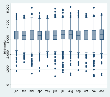
Figure 1: Box plots for birthweight by birth month

3.2 Multiple regressions

Through multiple linear regressions performed separately for gestational age and birthweight, it is possible to discover some significant associations with the covariates of Table 1. As shown in Tables 2 and 3 respectively, the number of gestational weeks and the weight of the infant tend to decrease as the woman age increases. As concerns the gestational age, we observe a significant association with citizenship, with women coming from foreign countries tending to deliver before Italian women. No other significant effect emerges with for the other covariates.

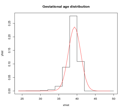
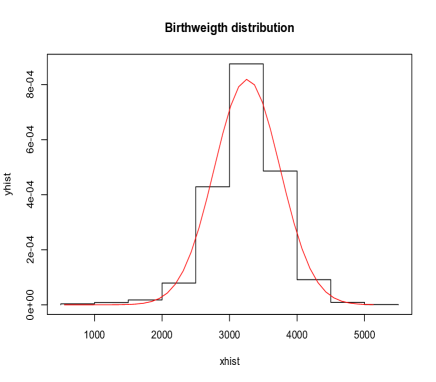
Figure 2: Histogram and normal curve for gestational age (left) and birthweight (right)

Figure 3: Scatter plot: birthweight versus gestational age

Some differences exist in the associative relations between birthweight and the covariates. The statistical effect of citizenship is significant at $10\%$ level for east-European women and at $5\%$ level for other citizenships (with respect to Italian citizenship); the birthweight results greater for east-European women with respect to Italians and smaller for the other citizenships. We also observe a significant association between birthweight and educational level: as expected, the higher the educational level, the greater the birthweight. Finally, some evidence of association is observable for the marital status: not married women give birth to infants with a lower weight with respect to married women.

covariate	category	est.	s.e.	$t$ stat.	$p$-value
intercept	–	39.325	0.051	772.686	0.000
age	–	-0.019	0.004	-4.910	0.000
age2	–	-0.001	0.001	-1.336	0.181
citizenship	Italian	0.000	–	–	–
citizenship	east-Europa	-0.242	0.059	-4.099	0.000
citizenship	other citizenship	-0.208	0.072	-2.887	0.004
education	middle school or less	0.000	–	–	–
education	high school	0.077	0.049	1.551	0.121
education	degree or above	0.077	0.057	1.345	0.179
marital	married	0.000	–	–	–
marital	not married	-0.025	0.039	-0.640	0.522

Table 2: Regression results for the gestational age

covariate	category	est.	s.e.	$t$ stat.	$p$-value
intercept	–	3.240	0.015	220.413	0.000
age	–	-0.005	0.001	-4.159	0.000
age2	–	-0.000	0.000	-0.875	0.381
citizenship	Italian	0.000	–	–	–
citizenship	east-Europa	0.032	0.017	1.847	0.065
citizenship	other citizenship	-0.050	0.021	-2.414	0.016
education	middle school or less	0.000	–	–	–
education	high school	0.032	0.014	2.243	0.025
education	degree or above	0.050	0.017	3.033	0.002
marital	married	0.000	–	–	–
marital	not married	-0.019	0.011	-1.682	0.092

Table 3: Regression for the birthweight

The results obtained by the multiple linear regressions suggest to proceed in the analysis investigating the causal relationships between variables. For this aim, we adopt a SEM framework that will be illustrated in the next section.

4 Proposed approach

In the following, we resume the conceptual framework described in Section 2 and we describe in more detail the resulting statistical model which is used to analyze possible effects of social characteristics of women on the inequalities in gestational age and birthweight of infants. We first present some preliminary concepts about causality. Secondly, we describe the adopted SEM, which is distinguished with respect to standard SEMs for two main elements: (i) it is based on the presence of a discrete, rather than continuous, latent variable and (ii) it accommodates for any type of responses rather than only for continuous responses. After having described the structural equations of the proposed model, we illustrate maximum likelihood estimation of their parameters.

4.1 Preliminaries on causality

One of the main reasons of systematic bias, which may lead to a wrong causal analysis and is commonly encountered in observational studies, is the presence of confounding effects that are ignored during the analysis (Hernan and Robins,, 2012). We speak about confounding effect (Freedman,, 1999) when two variables $z$ and $y$ have a common cause $u$, that confounds the true relationship between the putative cause $z$ and the effect $y$ (Figure 4 panel (a)). A typical situation takes place when a strong observed association between variables $z$ and $y$ may be explained partly or completely by controlling for the common cause $u$. On the other hand, we can also encounter the opposite situation when the true causal relationship between $z$ and $y$ is balanced and cancelled (so that $z$ and $y$ result statistically independent) by a relationship of equal strength but opposite sign due to the common cause $u$. In all these cases, it is important to take explicitly into account all the possible sources of heterogeneity of $y$, in order to avoid confounding effects.

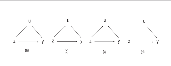
Figure 4: Causal relation between $z$ and $y$ and presence of a third variable $u$: (a) $u$ as common cause, (b) $u$ as intermediate effect, (c) $u$ as common effect, (d) $u$ as cause acting independently from $z$

Before proceeding, it is useful to point out that the presence of a common cause of both $z$ and $y$ is the main situation that requires a statistical adjustment. In fact, there are several situations that may confuse the researcher by leading to unnecessary or improper adjustments for a third variable. One case is encountered when variable $u$ has an intermediate effect along the pathway from $z$ to $y$ (Figure 4 panel (b)). Controlling for $u$ may be advised if we are interested in the direct effect of $z$ on $y$ (i.e., that part of effect not mediate through $u$), although it could be quite problematic (Freedman,, 1999; Greenland et al.,, 1999; Cox and Wermuth,, 2004). On the other hand, adjustment is useless if we are interested in the total effect of $z$ on $y$. As outlined in Section 2, this is the case with some variables in our study, such as IUGR.

Another situation takes place when both $z$ and $y$ have a common effect $u$ (Figure 4 panel (c)): as outlined by Greenland et al., (1999), in this case adjustment for $u$ “is not only unnecessary but irremediably harmful”, as it would result in the so-called adjustment-induced bias.

A final naive situation is illustrated in Figure 4 panel (d), where two causes of $y$ act independently one another (as shown through the missing edge between $z$ and $u$). Therefore, if our interest is limited to the causal effect of $z$ on $y$, ignoring $u$ has no consequences.

4.2 Preliminaries on structural equation models and extensions

As mentioned in Section 1, an useful statistical instrument to control for confounding bias is represented by SEMs (Wright,, 1921; Goldberger,, 1972; Duncan,, 1975; Bollen et al.,, 2008). As discussed by Pearl, (1998, 2009, 2011) and shown in detail by Cox and Wermuth, (2004), the partial regression coefficients of a SEM can be appropriately interpreted in terms of causal effects on the response variable, given that all the relevant background variables have been included in the model. This point represents one of the major difficulties for the causal analysis. Indeed, as outlined by Muthén, (1989), after having controlled for the observed covariates, the residual unexplained heterogeneity in the sample may be still substantial. Two main solutions have been proposed in the literature to treat this problem: (i) one is based on the introduction of a continuous latent effect that assumes different parameters at individual level (Ansari et al.,, 2000) and (ii) the other one, which is of interest in our contribution, is based on the assumption that the unobserved heterogeneity may be captured by a limited number of (unobserved) groups or classes of individuals. This latter approach is known as finite mixture SEM and it was introduced independently by Jedidi et al., (1997), Dolan and van der Maas, (1998), and Arminger et al., (1999). See also Vermunt and Magidson, (2005) for a clear illustration of different aspects, such as model specification without and with covariates, estimation, and model selection, and see Muthén, (2002) for a wide overview and classification of different types of SEM. More precisely, in a finite mixture SEM a different SEM may be specified for each mixture component, so that different components are allowed to have different parameter values and even different model types. In particular, we introduce in each structural equation a discrete latent variable $u$, the distribution of which is based on $K$ support points with specific mass probabilities. In this way, $u$ represents a common cause for all the responses. Moreover, the model we propose is configured as a special case of finite mixture SEM. Indeed, we assume that the $K$ latent classes differ one another for different intercepts, while the functional form of each regression equation and the values of structural coefficients are assumed to be constant among the classes.

With respect to standard SEMs that are based on continuous latent variables, the extension to the finite mixture approach presents some advantages. Firstly, each mixture component identifies homogeneous classes of individuals that have very similar latent characteristics, so that, in a decisional context, individuals in the same latent class will receive the same treatment (Lazarsfeld,, 1950; Lazarsfeld and Henry,, 1968; Goodman,, 1974). Moreover, this assumption allows to estimate the SEM in a semi-parametric way, namely without formulating any parametric assumption on the latent variable distribution.

Another useful extension of the standard SEM approach, that is considered in the present papers, derives from the observation that, in their original formulation, SEMs are based on continuous observed variables, so accommodating only a few types of application. A more general framework is obtained by adopting a generalized formulation (Skrondal and Rabe-Hesketh,, 2004, 2005; Bollen et al.,, 2008), which allows to take into account mixed types of response, that is both continuous and ordinal or binary observed responses, in the same set of structural equations. In this regards, since among the putative causes we have categorical variables for the educational level (with categories: 1 for middle school or less, 2 for high school, and 3 for degree or above) and the marital status (with categories: 0 for married, 1 for not married), we introduce a latent continuous variable $z_{il}^{*}$ underlying each observable variable $z_{il}$. In particular, we assume that

$$z_{il}=G_{l}(z_{il}^{*}),$$

where $G_{l}(\cdot)$ is a function which may depend on specific parameters according to the different nature of $z_{il}$. We consider the following cases:

• when the observed response is of a continuous type, an identity function is adopted, that is $G_{l}(z_{il}^{*})=z_{il}^{*}$;

• when the observed response is binary (i.e., $z_{il}=0,1$), then

  $$G_{l}(z_{il}^{*})=I\{z_{il}^{*}>0\},$$ (1)

  where $I\{\cdot\}$ is the indicator function assuming value 1 if its argument is true and zero otherwise;

• when the observed response is ordinal with categories $j=1,\ldots,J_{l}$, we introduce a set of cut-points $\tau_{l1}\geq\ldots\geq\tau_{l,J_{l}-1}$ and we define

  $$G_{l}(z_{il}^{*})=\left\{\begin{array}[]{cc}1&z_{il}^{*}\leq-\tau_{l1},\\ 2&-\tau_{l1}<z_{il}^{*}\leq-\tau_{l2},\\ \vdots&\vdots\\ J&z_{il}^{*}>-\tau_{l,J_{l}-1}.\end{array}\right.$$ (2)

4.3 The proposed finite mixture SEM

In the following, coherently with the theoretical model illustrated in Section 2 and in accordance with the notation previously introduced, the assumed causal relationships among the considered variables are expressed through a SEM composed by $3$ equations for each of the $n$ singleton delivers in the dataset. Two of these equations are referred to the causes educational level ($z_{i1}$) and marital status ($z_{i2}$), whereas the third one refers to the two correlated birth variable outcomes: gestational age ($y_{i1}$) and birthweight ($y_{i2}$). Moreover, the vector $\mbox{\boldmath$x$}_{i}$ is composed by observations on the variables age and squared age (both centered with respect to the mean value), and on dummies referred to citizenship (Italian is the reference category).

For every deliver $i$, $i=1,\ldots,n$, the generalized linear structural equations are as follows:

• Equation 1 (educational level): we assume that $z_{i1}=G_{1}(z_{i1}^{*})$, with $G_{1}$ defined as in (2) and

  $$z_{i1}^{*}=\mu_{1}+\alpha_{i1}+\mbox{\boldmath$x$}_{i}^{\prime}\mbox{\boldmath$\beta$}_{1}+\varepsilon_{i1},$$ (3)

  where $\mu_{1}+\alpha_{i1}$ is a specific intercept for subject $i$, $\mbox{\boldmath$\beta$}_{1}$ is a vector of regression coefficients for the covariates in $\mbox{\boldmath$x$}_{i}$, and $\varepsilon_{i1}$ is a random error term with logistic distribution;

• Equation 2 (marital status): we assume that $z_{i2}=G_{2}(z_{i2}^{*})$, with $G_{2}$ defined as in (1) and

  $$z_{i2}^{*}=\mu_{2}+\alpha_{i2}+\mbox{\boldmath$x$}_{i}^{\prime}\mbox{\boldmath$\beta$}_{2}+z_{i1}^{\prime}\gamma+\varepsilon_{i2},$$ (4)

  where $\mu_{2}+\alpha_{i2}$ is the subject specific intercept, $\mbox{\boldmath$\beta$}_{2}$ and $\gamma$ are regression coefficients, and $\varepsilon_{i2}$ is an error term with logistic distribution, which is independent of $\varepsilon_{i1}$;

• Equation 3 (gestational age, birthweight): in this case the observable variables, that we collect in the vector $\mbox{\boldmath$y$}_{i}=(y_{i1},y_{i2})^{\prime}$, are continuous and then we directly assume that

  $$\mbox{\boldmath$y$}_{i}=\mbox{\boldmath$\nu$}+\mbox{\boldmath$\delta$}_{i}+\mbox{\boldmath$\Phi$}\mbox{\boldmath$x$}_{i}+\mbox{\boldmath$\Psi$}\mbox{\boldmath$z$}_{i}+\mbox{\boldmath$\eta$}_{i},$$ (5)

  where $\mbox{\boldmath$\nu$}=(\nu_{1},\nu_{2})^{\prime}$, $\mbox{\boldmath$\delta$}_{i}=(\delta_{i1},\delta_{i2})^{\prime}$, $\mbox{\boldmath$\Phi$}=(\mbox{\boldmath$\phi$}_{1},\mbox{\boldmath$\phi$}_{2})^{\prime}$, $\mbox{\boldmath$\Psi$}=(\mbox{\boldmath$\psi$}_{1},\mbox{\boldmath$\psi$}_{2})^{\prime}$, and $\mbox{\boldmath$\eta$}=(\eta_{1},\eta_{2})^{\prime}$; the last is a vector of error terms, which is assumed to follow a bivariate Normal distribution centered at $\mathrm{𝟎}$ and with variance-covariance matrix $\Sigma$ and to be independent of the previous error terms. Here, we have two subject-specific intercepts, that is $\nu_{1}+\delta_{i1}$ for the gestational age and $\nu_{2}+\delta_{i2}$ for the birthweight. Accordingly, we have specific regression coefficients which are collected in $\mbox{\boldmath$\phi$}_{1}$ and $\mbox{\boldmath$\psi$}_{1}$ for the first response variable and in $\mbox{\boldmath$\phi$}_{2}$ and $\mbox{\boldmath$\psi$}_{2}$ for the second one.

Commenting the above equations, we note that the parameters of most interest in the present causal analysis are the regression coefficients in $\Psi$. Moreover, concerning the individual-specific parameters $\alpha_{i1}$, $\alpha_{i2}$, and $\mbox{\boldmath$\delta$}_{i}$, we clarify that, due to the latent class assumptions described in the previous section, these parameters have a discrete distribution with $K$ support points and corresponding probabilities (or weights). In particular, for the $k$-th class, with $k=1,\ldots,K$, the support points for $\alpha_{i1}$ and $\alpha_{i2}$ are denoted by $\xi_{k1}$ and $\xi_{k2}$ respectively, whereas the vector of support points for $\mbox{\boldmath$\delta$}_{i}$ is denoted by $\mbox{\boldmath$\zeta$}_{k}$; the corresponding weight is denoted by $\pi_{k}$. Support points and class weights are estimated on the basis of the data, together with the other parameters involved in the previous structural equations.

In order to make the model identifiable, the support points are suitably constrained by fixing their (weighted) mean at 0, so that $\mu_{1}$, $\mu_{2}$, and $\nu$ have the role average of intercepts. Note that, in order to make the model identifiable, we also constraint the first cutpoint involved in the second equation ($\tau_{21}$) to be equal to 0.

Finally, about the error terms involved in the three equations, we note that $\varepsilon_{1}$ and $\varepsilon_{2}$ are assumed to have a logistic distribution. Then, due to the specified $G_{l}(\cdot)$ functions, a global (or cumulative proportional odds) logit parameterization, used in the proportional-odds model of McCullagh, (1980), results for the conditional distribution of $z_{i1}$, whereas a standard logit parametrization results for $z_{i2}$; see also Agresti, (2002). In fact, we have that

$$\log\frac{p(z_{i1}\geq j|\alpha_{i1},\mbox{\boldmath$x$}_{i})}{p(z_{i1}<j|\alpha_{i1},\mbox{\boldmath$x$}_{i})}=\mu_{1}+\tau_{1,j-1}+\alpha_{i1}+\mbox{\boldmath$x$}_{i}^{\prime}\mbox{\boldmath$\beta$}_{1},\quad j=2,3,$$ (6)

and

$$\log\frac{p(z_{i2}=1|\alpha_{i2},\mbox{\boldmath$x$}_{i},z_{i1})}{p(z_{i2}=0|\alpha_{i2},\mbox{\boldmath$x$}_{i},z_{i1})}=\mu_{2}+\alpha_{i2}+\mbox{\boldmath$x$}_{i}^{\prime}\mbox{\boldmath$\beta$}_{2}+z_{i1}^{\prime}\mbox{\boldmath$\gamma$}.$$ (7)

Note that, we could also assume that both $\varepsilon_{1}$ and $\varepsilon_{2}$ have a Normal distribution, resulting in a parametrization based on probits and ordered probits, but this would have small impact on the model specification, while making the estimation more complex. On the other hand, given the nature of the variables in $\mbox{\boldmath$y$}_{i}$, it is obvious to assume a bivariate Normal distribution in the third equation for $\mbox{\boldmath$y$}_{i}$. Note, in particular, that this distribution depends on the variance-covariance matrix

$$\mbox{\boldmath$\Sigma$}=\left[\begin{array}[]{cc}\sigma_{1}^{2}&\sigma_{12}\\ \sigma_{21}&\sigma_{2}^{2}\\ \end{array}\right],$$

where $\sigma_{1}^{2}$ is the variance of $y_{1}$, $\sigma_{2}^{2}$ is the variance of $y_{2}$, and $\sigma_{12}=\sigma_{21}$ is the covariance between $y_{1}$ and $y_{2}$. All are free parameters and then we allow a free correlation, which is measured by the index

$$\rho=\frac{\sigma_{12}}{\sqrt{\sigma_{1}^{2}\sigma_{2}^{2}}},$$

between the two variables, even given the observable and the unobservable variables.

4.4 Model estimation

We perform estimation of the parameters of the model previously introduced by the maximum likelihood method. This requires to derive the joint distribution of ($z_{i1},z_{i2},\mbox{\boldmath$y$}_{i}$), that is the conditional distribution of these variables given $\mbox{\boldmath$x$}_{i}$, once the individual-specific parameters $\alpha_{i1}$, $\alpha_{i2}$, and $\mbox{\boldmath$\delta$}_{i}$ have been integrated out. This distribution may be expressed as a finite mixture, that is

$$f(z_{i1},z_{i2},\mbox{\boldmath$y$}_{i}|\mbox{\boldmath$x$}_{i})=\sum_{k=1}^{K}\pi_{k}p(z_{i1}|\alpha_{i1}=\xi_{k1},\mbox{\boldmath$x$}_{i})p(z_{i2}|\alpha_{i2}=\xi_{k2},\mbox{\boldmath$x$}_{i},z_{i1})f(\mbox{\boldmath$y$}_{i}|\mbox{\boldmath$\delta$}_{i}=\mbox{\boldmath$\zeta$}_{k},\mbox{\boldmath$x$}_{i},\mbox{\boldmath$z$}_{i}),$$

where the probabilities mass function for $z_{i1}$ and $z_{i2}$ are defined through (6) and (7), whereas $f(\mbox{\boldmath$y$}_{i}|\mbox{\boldmath$\delta$}_{i}=\mbox{\boldmath$\zeta$}_{k},\mbox{\boldmath$x$}_{i},\mbox{\boldmath$z$}_{i})$ is the density function, computed at $\mbox{\boldmath$y$}_{i}$, of a bivariate normal distribution with mean $\mbox{\boldmath$\nu$}+\mbox{\boldmath$\delta$}_{i}+\mbox{\boldmath$\Phi$}\mbox{\boldmath$x$}_{i}+\mbox{\boldmath$\Psi$}\mbox{\boldmath$z$}_{i}$ and variance-covariance matrix $\Sigma$; see equation (5).

Under the assumption that the sample units are independent each other, the log-likelihood of the model to be maximized for the estimation is

$$\ell(\mbox{\boldmath$\theta$})=\sum_{i=1}^{n}\log f(z_{i1},z_{i2},\mbox{\boldmath$y$}_{i}|\mbox{\boldmath$x$}_{i}),$$

with $\theta$ denoting the vector of all model parameters. Maximization of $\ell(\mbox{\boldmath$\theta$})$ may be efficiently performed through an Expectation-Maximization (EM) algorithm (Dempster et al.,, 1977). In the following, we sketch this algorithm, referring to more specialized papers on the topic; see, for instance, Bartolucci and Forcina, (2006) and the references therein. Moreover, as already mentioned, for the present application we implemented the algorithm in a set of R functions that we make available to the reader upon request.

The EM algorithm is based on the so-called complete data log-likelihood, which could be computed if we knew the latent class to which every sample unit belongs. This function may be expressed as

$$\ell^{*}(\mbox{\boldmath$\theta$}) = \sum_{k=1}^{K}\sum_{i=1}^{n}w_{ik}\log[p(z_{i1}|\alpha_{i1}=\xi_{k1},\mbox{\boldmath$x$}_{i})p(z_{i2}|\alpha_{i2}=\xi_{k2},\mbox{\boldmath$x$}_{i},z_{i1})f(\mbox{\boldmath$y$}_{i}|\mbox{\boldmath$\delta$}_{i}=\mbox{\boldmath$\zeta$}_{k},\mbox{\boldmath$x$}_{i},\mbox{\boldmath$z$}_{i})]+$$ (8)

$$+ \sum_{k=1}^{K}\sum_{i=1}^{n}w_{ki}\log\pi_{k},$$

where $w_{ik}$ is a dummy variable equal to 1 if unit $i$ belongs to subject $k$ and to 0 otherwise. Based of this function, the EM algorithm alternates the following two steps until convergence in $\ell(\mbox{\boldmath$\theta$})$:

• step E: compute the conditional expected value of $\ell^{*}(\mbox{\boldmath$\theta$})$ given the observed data and the current value of the parameters in $\theta$; this is equivalent to substituting every dummy variable $w_{ik}$ in (8) by the corresponding conditional expected value

  $$\hat{w}_{ik}=\frac{\pi_{k}p(z_{i1}|\alpha_{i1}=\xi_{k1},\mbox{\boldmath$x$}_{i})p(z_{i2}|\alpha_{i2}=\xi_{k2},\mbox{\boldmath$x$}_{i},z_{i1})f(\mbox{\boldmath$y$}_{i}|\mbox{\boldmath$\delta$}_{i}=\mbox{\boldmath$\zeta$}_{k},\mbox{\boldmath$x$}_{i},\mbox{\boldmath$z$}_{i})}{f(z_{i1},z_{i2},\mbox{\boldmath$y$}_{i}|\mbox{\boldmath$x$}_{i})};$$

• step M: maximize the expected value of $\ell^{*}(\mbox{\boldmath$\theta$})$ obtained above with respect to the model parameters; to update the class weights we have an explicit solution given by

  $$\pi_{k}=\frac{\sum_{i=1}^{n}\hat{w}_{ik}}{n},\quad k=1,\ldots,K.$$

  Moreover, for the parameters involved in (3) and (4) we use simple iterative algorithms that are currently used to maximize the weighted log-likelihood of a proportional odds model (McCullagh,, 1980), whereas the parameters in equation (5) are updated by solving a weight least square problem.

The value of $\theta$ at convergence of the EM algorithm is taken as the maximum likelihood estimate of this parameter vector, denoted by $\hat{\mbox{\boldmath$\theta$}}$. To treat the well-known problem of multi-modality of likelihood characterizing finite mixture and latent variable models, we suggest to initialize the estimation algorithm by both deterministic and random starting values. Finally, standard errors for the parameter estimates are obtained by inversion of the observed information matrix, which is numerically obtained from the score function that, in turn, is obtained by exploying a result due to Oakes, (1999).

5 Results

In the following, we illustrate the results obtained through the finite mixture SEM presented in the previous section and applied to the dataset about the 9,005 newborns collected in the Region of Umbria; see Section 3.1 for a description of the dataset. Firstly, we give the results about the selection process of the optimal number of latent classes (Table 4). Secondly, the estimated regression coefficients are reported separately for each structural equation in Tables 5, 6, and 7. Finally, the adopted latent structure is described in Table 8, which shows the estimated support points for each latent class and the corresponding weights.

First of all, in applying the proposed finite mixture approach, the choice of the optimal number of latent classes $K$ is of crucial importance. For this aim, several studies (Roeder and Wasserman,, 1997; Dasgupta and Raftery,, 1998; McLachlan and Peel,, 2000) conclude that the Bayesian Information Criterion (BIC; Schwarz,, 1978) present an adequate performance for choosing $K$. We remind that this criterion is based on penalizing the maximum value of the log-likelihood $\hat{\ell}$ by a term depending on the number of free parameters ($\#\mathrm{par}$) and on the sample size ($n$):

$$\mathrm{BIC}=-2\hat{\ell}+\log(n)\#\mathrm{par}.$$

In practice, we fit the adopted SEM with increasing $K$ values, relying the choice of optimal $K$ on the value just before the first increasing of the BIC index. On the basis of results shown in Table 4, we obtain the minimum BIC value in correspondence of $K=3$ latent classes.

$K$	$\hat{\ell}$	$\#$par	BIC
1	-35700.768	32	71692.914
2	-34536.422	37	69409.750
3	-34488.589	42	69359.610
4	-34467.548	47	69363.055

Table 4: Results from the preliminary fitting: number of mixture components ($K$), maximum log-likelihood ($\hat{\ell}$), number of parameters ($\#$par), and BIC index

We now consider the estimates for the structural equations (3) and (4) about education and marital status, respectively. In particular, we observe that the educational level significantly increases with the age of the woman and it is lower for foreigners with respect to Italians (Table 5). Effects of age and citizenship are also highly significant with reference to the marital status (Table 6): the probability to be married increases with age and it is higher for foreign women. Moreover, a causal effect of educational level on marital status is detected after controlling for the latent classes: higher the educational level, higher the probability to be married.

covariate	category	est.	s.e.	$t$ stat.	$p$-value
intercept ($\mu_{1}$)	–	2.053	0.039	52.285	0.000
1st cutpoint ($\tau_{1}$)	–	0.000	–	–	–
2st cutpoint ($\tau_{2}$)	–	-2.695	0.031	-20.780	0.000
age	–	0.103	0.004	23.405	0.000
age2	–	-0.009	0.001	-14.587	0.000
citizenship	Italian	0.000	–	–	–
citizenship	east-Europa	-0.806	0.069	-11.712	0.000
citizenship	other citizenship	-1.100	0.086	-12.780	0.000

Table 5: Regression results for educational level

covariate	category	est.	s.e.	$t$ stat.	$p$-value
intercept ($\mu_{2}$)	–	-0.763	0.065	-11.313	0.000
age	–	-0.027	0.005	-5.487	0.000
age2	–	0.008	0.001	12.381	0.000
citizenship	Italian	0.000	–	–	–
citizenship	east-Europa	-0.679	0.082	-8.264	0.000
citizenship	other citizenship	-0.677	0.101	-6.701	0.000
education	middle school or less	0.000	–	–	–
education	high school	-0.152	0.064	-2.375	0.018
education	degree or above	-0.468	0.076	-6.123	0.000

Table 6: Regression results for marital status

We now analyze the results shown in Table 7 about the outcome variables, according to the formulation of equation (5). Both gestational age and birthweight decrease as mother’s age increases, while the association with citizenship is something different. Women from east-Europa deliver significantly before Italians, but their newborns have a higher weight. On the other hand, women from other countries present differences on both response variables with respects to Italian women.

response var.	covariate	category	est.	s.e.	$t$ stat.	$p$-value
Gestational age	intercept ($\nu_{1}$)	–	39.346	0.044	905.935	0.000
	age	–	-0.015	0.003	-4.789	0.000
	age2	–	-0.001	0.000	-2.544	0.011
	citizenship	Italian	0.000	–	–	–
	citizenship	east-Europa	-0.194	0.049	-3.942	0.000
	citizenship	other citizenship	-0.112	0.060	-1.855	0.064
	education	middle school or less	0.000	–	–	–
	education	high school	0.025	0.042	0.608	0.543
	education	degree or above	0.029	0.049	0.600	0.548
	marital	married	0.000	–	–	–
	marital	not married	0.025	0.033	0.749	0.454
Birthweight	intercept ($\nu_{2}$)	–	3.238	0.017	195.392	0.000
	age	–	-0.004	0.001	-3.863	0.000
	age2	–	-0.000	0.000	-1.708	0.088
	citizenship	Italian	0.000	–	–	–
	citizenship	east-Europa	0.041	0.016	2.653	0.008
	citizenship	other citizenship	-0.031	0.019	-1.608	0.108
	education	middle school or less	0.000	–	–	–
	education	high school	0.023	0.014	1.674	0.094
	education	degree or above	0.043	0.017	2.462	0.014
	marital	married	0.000	–	–	–
	marital	not married	0.011	0.012	0.904	0.366
	variance of gestational age ($\sigma_{1}^{2}$)		1.776
	variance of birthweight ($\sigma_{2}^{2}$)		0.171
	covariance ($\sigma_{12}$)		0.248
	correlation ($\rho_{12}$)		0.450

Table 7: Regression results for the gestational age and the birthweight

By comparing Table 7 with Tables 2 and 3, it is possible to draw some conclusions about the causal effects of educational level and marital status on the birth outcomes. About the marital status, the analysis confirms the absence of any causal effect. With reference to the educational level, the increase of $p$-values denote the presence of a confounding effect. However, even after controlling for a latent common cause, a significative effect persists on the birthweight: a higher educational level causes a higher birthweight. Note that the causal effect is well defined for the degree or above modality, with a $p$-value equal to $0.014$, while this is not longer true for mothers with a high school. Moreover, we observe that correlation between outcomes is not enough large ($\rho_{12}=0.45$). Given that gestational age and birthweight are conditioned to covariates and latent variables, this is compatible with causes affecting in a different way the two outcomes.

We now analyze the results concerning the latent structure of the model (Table 8). As mentioned above, $K=3$ different latent classes are detected. Note that the estimated $p$-values refer to the comparisons between classes 2 or 3 versus class 1. The most representative class is the first one, to which corresponds a weight equal to ${\pi}_{1}=0.931$, whereas the remaining part of women results assigned to the third class with ${\pi}_{3}=0.041$ and to the second class with ${\pi}_{2}=0.028$.

	$k=1$	$k=2$	$k=3$
education ($\xi_{k1}$)	0.005	-0.165 (0.234)	-0.005 (0.964)
marital status ($\xi_{k2}$)	0.026	0.289 (0.081)	-0.794 (0.021)
gestational age ($\zeta_{k1}$)	0.178	-6.086 (0.000)	0.123 (0.671)
birthweight ($\zeta_{k2}$)	0.005	-1.245 (0.000)	0.728 (0.000)
class weight ($\pi_{k}$)	0.931	0.028	0.041

Table 8: Class weights and support points estimates (p-values in parenthesis are referred to the comparison between the second and third class with the first class)

With a weight greater than 0.90, women belonging to class 1 represent the main part of the population, so that no particular difference results with respect to the average values of the entire population, as shown by the estimated support points which very close to zero.

Differently, women from class 2 result to be well characterized. With a support point equal to 0.289, to which correspond an odds equal to $\exp(0.289)=1.335$, women in class 2 present a significant higher propensity (at $10\%$ level) to be not married with respect to women in the first class. On average they give birth 6.1 weeks before and their infants weigh 1.245 kg less. No significant difference results about the educational level. Finally, women in class 3 have a higher tendency to be married (odds equal to $\exp(-0.794)=0.452$ for not being married) and the birthweight of her infants is significantly higher ($+0.728$ kg with respect to the first class). On the other hand, no significant difference results with respect to educational level and gestational age.

Our estimates allow us to assess potential heterogeneity in infant health outcomes of educational attainments across mothers. We focus our attention on birthweight because, differently from recent findings of this literature, education does not find significant estimates for gestational age. The estimates suggest that higher education increases birthweight by a significant, although quantitatively not large, amount: a graduate mother increases, on average, of 43 gr the newborn weight with respect to mothers with a basic educational level. This impact on birthweight is more limited for mothers that only achieve a high school level; it mostly cast some doubt if the estimated parameters may or may not impact on child health, because the significance is between 5% and 10% level. Three facts stand out from our results, as we explain in the following.

First, the finite mixture SEM estimates for the effect of education on birthweight are lower than standard regression ones (and with higher $p$-values), a finding common to studies similar to ours (Abrevaya and Dahl,, 2008), and in line with the a priori that upward bias in regression estimates are driven by the correlation between mother’s education and unobserved variables.

Second, the finite mixture SEM suggests a significant and positive effect of education on the probability to be married. Specifically, non-completing high school or degree would lower the mother probability to be married of about 14% and 37%, respectively. While the range of variation of these estimates may reflect the specificity of our sample, we note that in most cases they are against the estimates reported in this specific literature. See, for example, Breierova and Duflo, (2004) for a study in Indonesia and Lefgren and McIntyre, (2006) for a study in the US. As known, based on catholic background of marriage, the postponement of mother with higher education in Italy does not influence their propensity towards traditional cohabitation.

Third, the estimated effect of the latent classes stems qualitatively almost exclusively from differences between married and not married mothers or, alternatively, within the married group.

Different arguments may help to explain the first result. The prevalent interpretation is that the woman’s educational level may be related with specific unobservable variables, such as the ability to properly manage the pregnancy so as to improve the health level of the newborn. This implies that an upward bias emerges in the regression estimates, a result consistent with the findings of Table 4. On the other hand, unlike Abrevaya and Dahl, (2008), we find a greter effect on birthweight for mothers with the highest level of education (with respect to women with a high school degree), a result qualitatively in accordance with Currie and Moretti, (2003). Note that, if birthweight responds to educational level, conditionally on to be married or not, unobservable factors linked with her husband may further affect the results, although latent classes have been identified. We will return to this discussion below, when we attempt to identify a latent class by a positive assortative mating within married mothers.

Despite a growing literature, little is known about to the causal effect of the woman’s educational level on her marital status. Our estimates indicate that the education level has a positive impact on the marriage probability, especially with an educated potential partner. This is clearly not in line with the results of Breierova and Duflo, (2004), in which an increase of education does not lead to a significant impact on the probability of a woman being currently married. Although there are several respects in which the increase in the marriage chance is consistent with a higher level of education, we can conjecture that our data are in line with the hypothesis that this effect is mitigated by the specificity of the Italian labor market. The job participation rate of the mothers in our sample is close to that of the national mean of about 45%, an index distant of more than 10 percentage points from the average of the EU countries and far from the aims of European Pact for gender equality. In addition, this is heterogeneous across levels of education. In fact, if we refer to mothers with at least a degree before the first pregnancy, the Italian participation rate is even much lower. In contrast to the classical predictions in terms of incentive marriage (Lam,, 1988), this low participation rate of women may induce potential gains from household specialization. The result reinforces the known evidence that more educated mothers use the status to be married to postpone the job search or to avoid to select jobs that are not in accordance to their individual expectations, a finding not in contrast with the stylized fact that, over the life cycle, more educated mothers have on average a higher participation rate.

By acquiring the highest educational level, a mother can affect the identity of his future husband. However, the identification of the effect of education on the probability to be married and outcomes at birth is complicated by the endogeneity involved in the partner’s educational level, that may affect mothers’ choices and outcomes; that is, marriages may well be determined by factors such as social background and geographical location. These factors are also correlated with education, and could lead the observed correlation in spouses’ education to be partly or entirely spurious. We have recognized above that the last latent class includes women with a higher chance to be married. The large and positive impact on birthweight of the third class may lead to assume a married mothers’ group with a positive assortative mating. Here, we indirectly investigate the latter effect by including in the finite mixture class SEM the father’s educational level as a potential confounder of the birthweight outcome and evaluate the sensitivity with respect to the main relationship between education and birthweight. Tables 9 and 10 shows the results of these estimates. Noticeable, the contribution of education on birth outcome becomes less susceptible to ambiguous conclusions. Causal effect of mother’s education with at least a degree are still significant and large enough to conclude over the goodness of the estimates, while it is even clearer that those with high school do not contribute to explain differences in the birthweight. Moreover, our findings appear first to support the idea that the mothers in class 3 have a positive assortative mating with a large effect on infant outcomes (compare $\hat{\gamma}_{32}$ of Table 10 with its analogous of Table 8), and to emphasize the robustness of our analysis, we note that all other estimated coefficients are close to the model presented in table 7.

response var.	covariate	category	est.	s.e.	$t$ stat.	$p$-value
Gestational age	intercept ($\nu_{1}$)	–	39.473	0.109	362.26	0.000
	education	middle school or less	0.000	–	–	–
	education	high school	0.012	0.043	0.27	0.787
	education	degree or above	0.021	0.053	0.40	0.690
	marital	married	0.000	–	–	–
	marital	not married	0.013	0.034	0.39	0.699
Birthweight	intercept ($\nu_{2}$)	–	3.263	0.115	28.54	0.000
	education	middle school or less	0.000	–	–	–
	education	high school	0.015	0.014	1.11	0.268
	education	degree or above	0.032	0.017	1.93	0.053
	marital	married	0.000	–	–	–
	marital	not married	-0.007	0.011	-0.69	0.489

Table 9: Regression results for the gestational age and the birthweight controlled for father’s educational level, age and citizenship

	k=1	k=2	k=3
gestational age ($\zeta_{k1}$)	0.173	-5.995 (0.000)	0.172 (0.993)
birthweight ($\zeta_{k2}$)	0.035	-1.215 (0.000)	0.036 (0.993)

Table 10: Support points estimates after controlling for father’s educational level (p-values in parenthesis)

6 Conclusions

The article presents new evidence on the child health increasing effect of education, using a finite mixture structural equation model (SEM) to identify a causal link. In particular, the estimation strategy controlling for the effects of marital status, observed and unobserved characteristics of the mother guarantees that health outcomes are entirely driven by differences in education. This is made possible by the inclusion of random parameters in each structural equation, which follow a discrete distribution with support points and weights estimated on the basis of the dataset. These support points then identify latent classes of individuals that allow us to adjust for unobserved confounding.

We report empirical findings showing that high education of mothers increases the birthweight whereas gestational age is not affected. The estimated social saving from birthweight increase, implied by our estimates, are substantial if associated to married mothers with positive assortative mating, that we identify through the latent classes.

The existence of a causal birthweight increasing effect of high education has potentially important implications for longer-term effort aimed at reducing the level of birthweight. Policies that incentive high school, as an investment in human capital, have significant potential to reduce the percentage of mothers that deliver children below the minimum threshold weight, by increasing skill levels in helping care and behaviors consistent with a healthy pregnancy. At the very least, our result confirm that improving education among young mothers should be viewed as a key policy to reduce costs of unhealthy child outcome, a finding that appear to be emphasized at the “family level” by the presence of a more educated husband.

References

- Abrevaya and Dahl, (2008) Abrevaya, J. and Dahl, C. M. (2008). The effects of birth inputs on birthweight. Journal of Business & Economic Statistics, 26:379–397.
- Agresti, (2002) Agresti, A. (2002). Categorical Data Analysis. John Wiley & Sons, Hoboken.
- Almond et al., (2005) Almond, D., Chay, K. Y., and Lee, D. S. (2005). The costs of low birth weight. The Quarterly Journal of Economics, 120(3):1031–1083.
- Almond et al., (2011) Almond, D., Currie, J., and Simeonova, E. (2011). Public vs. private provision of charity care? evidence from the expiration of hill-burton requirements in florida. Journal of Health Economics, 30(1):189–199.
- Ansari et al., (2000) Ansari, A., Jedidi, K., and Jagpal, S. (2000). A hierarchical bayesian methodology for treating heterogeneity in structural equation models. Marketing Science, 19(4):328 – 347.
- Arminger et al., (1999) Arminger, G., Stein, P., and Wittenberg, J. (1999). Mixtures of conditional mean- and covariance-structure models. Psychometrika, 64(4):475–494.
- Bartolucci and Forcina, (2006) Bartolucci, F. and Forcina, A. (2006). A class of latent marginal models for capture-recapture data with continuous covariates. Journal of the American Statistical Association, 101:786–794.
- Becker, (1981) Becker, G. S. (1981). Altruism in the family and selfishness in the market place. Economica, 48(189):1–15.
- Becker, (1985) Becker, G. S. (1985). Human capital, effort, and the sexual division of labor. Journal of Labor Economics, 3(1):S33–58.
- Behrman and Rosenzweig, (2002) Behrman, J. R. and Rosenzweig, M. R. (2002). Does increasing women’s schooling raise the schooling of the next generation? American Economic Review, 92(1):323–334.
- Bollen et al., (2008) Bollen, K., Rabe-Hesketh, S., and Skrondal, A. (2008). Structural equation models. In Box-Steffensmeier, J. M., Brady, H., and Collier, D., editors, Oxford Handbook of Political Methodology, chapter Structural equation models, pages 432–455. Oxford University Press.
- Breierova and Duflo, (2004) Breierova, L. and Duflo, E. (2004). The impact of education on fertility and child mortality: Do fathers really matter less than mothers? NBER Working Papers 10513, National Bureau of Economic Research, Inc.
- Case and Paxson, (2011) Case, A. and Paxson, C. (2011). The long reach of childhood health and circumstance: Evidence from the whitehall ii study. Economic Journal, 121(554):F183–F204.
- Chou et al., (2010) Chou, S.-Y., Liu, J.-T., Grossman, M., and Joyce, T. (2010). Parental education and child health: Evidence from a natural experiment in taiwan. American Economic Journal: Applied Economics, 2(1):33–61.
- Conti et al., (2010) Conti, G., Heckman, J., and Urzua, S. (2010). The education-health gradient. American Economic Review, 100(2):234–38.
- Cox and Wermuth, (2004) Cox, D. and Wermuth, N. (2004). Causality: a statistical view. International Statistical Review, 72(3):285–305.
- Currie, (2011) Currie, J. (2011). Inequality at birth: Some causes and consequences. American Economic Review, 101(3):1–22.
- Currie and Moretti, (2003) Currie, J. and Moretti, E. (2003). Mother’s education and the intergenerational transmission of human capital: Evidence from college openings. The Quarterly Journal of Economics, 118(4):1495–1532.
- Dasgupta and Raftery, (1998) Dasgupta, A. and Raftery, A. E. (1998). Detecting features in spatial point processes with cluster via model-based clustering. Journal of the American Statistical Association, 93:294–302.
- Dawid, (2002) Dawid, A. (2002). Influence diagrams for causal modelling and inference. International Statistical Review, 70:161 – 189.
- Dempster et al., (1977) Dempster, A. P., Laird, N. M., and Rubin, D. B. (1977). Maximum likelihood from incomplete data via the EM algorithm (with discussion). Journal of the Royal Statistical Society, Series B, 39:1–38.
- Dolan and van der Maas, (1998) Dolan, C. and van der Maas, H. (1998). Fitting multivariate normal finite mixtures subject to structural equation modeling. Psychometrika, 63(3):227–253.
- Duncan, (1975) Duncan, O. (1975). Introduction to structural equation models. Academic Press, New York.
- Freedman, (1999) Freedman, D. (1999). From association to causation: some remarks on the history of statistics. Statistical Science, 14(3):243–258.
- Goldberger, (1972) Goldberger, A. (1972). Structural equation models in the social sciences. Econometrica: Journal of Econometric Society, 40:979 – 1001.
- Goodman, (1974) Goodman, L. A. (1974). Exploratory latent structure analysis using both identifiable and unidentifiable models. Biometrika, 61:215–231.
- Greenland et al., (1999) Greenland, S., Pearl, J., and Robins, J. (1999). Causal diagrams for epidemiologic research. Epidemiology, 10:37 – 48.
- Hernan and Robins, (2012) Hernan, M. and Robins, J. (2012). Causal Inference. Chapman & Hall/CRC.
- Holland, (1986) Holland, P. (1986). Statistics and causal inference. Journal of American Statistical Association, 81:945–960.
- Jedidi et al., (1997) Jedidi, K., Jagpal, H., and DeSarbo, W. (1997). Stemm: a general finite mixture structural equation model. Journal of Classification, 14:23–50.
- Kramer, (1987) Kramer, M. S. (1987). ntrauterine growth and gestational duration determinants. Pediatrics, LXXX:502–511.
- Lam, (1988) Lam, D. (1988). Marriage markets and assortative mating with household public goods: Theoretical results and empirical implications. Journal of Human Resources, 23(4):462–87.
- Lauritzen, (1996) Lauritzen, S. (1996). Graphical models. Claredon Press, Oxford.
- Lazarsfeld, (1950) Lazarsfeld, P. F. (1950). The logical and mathematical foundation of latent structure analysis. In S. A. Stouffer, L. Guttman, E. A. S., editor, Measurement and Prediction, New York. Princeton University Press.
- Lazarsfeld and Henry, (1968) Lazarsfeld, P. F. and Henry, N. W. (1968). Latent Structure Analysis. Houghton Mifflin, Boston.
- Lefgren and McIntyre, (2006) Lefgren, L. and McIntyre, F. (2006). The relationship between women’s education and marriage outcomes. Journal of Labor Economics, 24(4):787–830.
- Lindeboom et al., (2009) Lindeboom, M., Llena-Nozal, A., and van der Klaauw, B. (2009). Parental education and child health: Evidence from a schooling reform. Journal of Health Economics, 28(1):109–131.
- McCrary and Royer, (2011) McCrary, J. and Royer, H. (2011). The effect of female education on fertility and infant health: Evidence from school entry policies using exact date of birth. American Economic Review, 101(1):158–95.
- McCullagh, (1980) McCullagh, P. (1980). Regression models for ordinal data (with discussion). Journal of the Royal Statistical Society, Series B, 42:109–142.
- McLachlan and Peel, (2000) McLachlan, G. and Peel, D. (2000). Finite mixture models. Wiley Series in Probability and Statistics.
- Muthén, (1989) Muthén, B. (1989). Latent variable modeling in heterogeneous populations. Psychometrika, 54:557 – 585.
- Muthén, (2002) Muthén, B. (2002). Beyond sem: general latent variable modeling. Behaviormetrika, 29(1):81–117.
- Neyman, (1923) Neyman, J. (1923). On the application of probability theory to agricultural experiments. essays on principles. section 9. Statistical Science, 5:465 – 480.
- Oakes, (1999) Oakes, D. (1999). Direct calculation of the information matrix via the EM algorithm. Journal of the Royal Statistical Society, Series B, 61:479–482.
- Pearl, (1998) Pearl, J. (1998). Graphs, causality, and structural equation models. Sociological methods and research, 27:226–284.
- Pearl, (2000) Pearl, J. (2000). Causality: models, reasoning, and inference. Cambridge University Press, New York.
- Pearl, (2009) Pearl, J. (2009). Causal inference in statistics: an overview. Statistics Surveys, 3:96–146.
- Pearl, (2011) Pearl, J. (2011). The causal foundations of structural equation modeling. In Hoyle, R., editor, Handbook of structural equation modeling. Guildford Press.
- Pencavel, (1998) Pencavel, J. (1998). Assortative mating by schooling and the work behavior of wives and husbands. American Economic Review, 88(2):326–29.
- Qian, (1998) Qian, Z. (1998). Changes in assortative mating: The impact of age and education, 1970-1990. Demography, 35(3):279–92.
- Roeder and Wasserman, (1997) Roeder, K. and Wasserman, L. (1997). Practical bayesian density estimation using mixtures of normals. Journal of the American Statistical Association, 92:894–902.
- Rosenzweig and Schultz, (1983) Rosenzweig, M. R. and Schultz, T. P. (1983). Estimating a household production function: Heterogeneity, the demand for health inputs, and their effects on birth weight. Journal of Political Economy, 91(5):723–46.
- Rosenzweig and Wolpin, (1991) Rosenzweig, M. R. and Wolpin, K. I. (1991). Inequality at birth : The scope for policy intervention. Journal of Econometrics, 50(1-2):205–228.
- Rubin, (1974) Rubin, D. (1974). Estimating causal effects of treatments in randomized and non randomized studies. Journal of Educational Psychology, 66:688 – 701.
- Schwarz, (1978) Schwarz, G. (1978). Estimating the dimension of a model. Annals of Statistics, 6(2):461–464.
- Skrondal and Rabe-Hesketh, (2004) Skrondal, A. and Rabe-Hesketh, S. (2004). Generalized Latent Variable Modeling: Multilevel, Longitudinal, and Structural Equation Models. Chapman & Hall/CRC.
- Skrondal and Rabe-Hesketh, (2005) Skrondal, A. and Rabe-Hesketh, S. (2005). Structural equation modeling: categorical variables. In Encyclopedia of Statistics in Behavioral Science. Wiley.
- Torche and Corvalan, (2010) Torche, D. and Corvalan, A. (2010). Seasonality of birth weight in chile: Environmental and socioeconomic factors. Annals of epidemiology, 20:818–826.
- Vermunt and Magidson, (2005) Vermunt, J. and Magidson, J. (2005). Structural equation models: mixture models. In Everitt, B. and Howell, D., editors, Encycopledia of Statistics in Behavioral Science, pages 1922–1927. Wiley.
- Weiss et al., (2009) Weiss, Y., Chiappori, P., and Iyigun, M. (2009). Investment in schooling and the marriage market. American Economic Review, 99(5).
- Wright, (1921) Wright, S. (1921). Correlation and causation. Journal of Agricultural Research, 20:557 – 585.