Long-term Radio Observations of the Intermittent Pulsar B1931$+$24

Abstract

We present an analysis of approximately 13-yr of observations of the intermittent pulsar B1931$+$24 to further elucidate its behaviour. We find that while the source exhibits a wide range of nulling ($\sim 4-39$ d) and radio-emitting ($\sim 1-19$ d) timescales, it cycles between its different emission phases over an average timescale of approximately 38 d, which is remarkably stable over many years. On average, the neutron star is found to be radio-emitting for $26\pm 6\,\%$ of the time. No evidence is obtained to suggest that the pulsar undergoes any systematic, intrinsic variations in pulse intensity during the radio-emitting phases. In addition, we find no evidence for any correlation between the length of consecutive emission phases. An analysis of the rotational behaviour of the source shows that it consistently assumes the same spin-down rates, i.e. $\dot{\nu}=-16\pm 1\times 10^{-15}$ s^-2 when emitting and $\dot{\nu}=-10.8\pm 0.4\times 10^{-15}$ s^-2 when not emitting, over the entire observation span. Coupled with the stable switching timescale, this implies that the pulsar retains a high degree of magnetospheric memory, and stability, in spite of comparatively rapid ($\sim$ ms) dynamical plasma timescales. While this provides further evidence to suggest that the behaviour of the neutron star is governed by magnetospheric-state switching, the underlying trigger mechanism remains illusive. This should be elucidated by future surveys with next generation telescopes such as LOFAR, MeerKAT and the SKA, which should detect similar sources and provide more clues to how their radio emission is regulated.

1 Introduction

PSR B1931$+$24 was discovered in 1985 with the NRAO 100-m Green Bank Telescope (Stokes et al., 1985). However, it was not until 13 years later, during routine pulsar timing observations at Jodrell Bank, that the remarkable properties of this object were noted. Unlike conventional nulling pulsars, which undergo temporary emission cessation (or pulse nulling) over timescales of $\lesssim 100$ pulse periods (e.g. Backer 1970; Ritchings 1976; Rankin 1986; Wang et al. 2007), PSR B1931$+$24 has been found to exhibit extremely long duration, active ($\sim 5-10$ d) and quiescent ($\sim 25-35$ d) radio emission phases. Remarkably, these emission phases also repeat quasi-periodically, are broadband in frequency and are found to be correlated with the rotational behaviour of the star. That is, the source exhibits a spin-down rate which is $\sim 50\,\%$ greater in the active (radio-on, hereafter) emission phases, compared with that of the non-radio emitting (radio-off, hereafter) phases (Kramer et al., 2006).

To date, a handful of similar objects have been discovered, e.g. PSR J1832$+$0029 (Lorimer et al., 2012) and PSR J1841$-$0500 (Camilo et al., 2012). Despite this, only the properties of PSR B1931$+$24 have been studied, or attempted to be explained, in some detail (see, e.g., Kramer et al. 2006; Cordes & Shannon 2008; Rea et al. 2008; Rosen et al. 2011; Li et al. 2012). As such, theories which attempt to explain the behaviour of such long-term intermittent pulsars are centred mainly on observations of this object, particularly those in the radio regime.

Amongst the most promising of these theories, is the possibility that the pulsar magnetosphere experiences systematic variation in its global charge distribution; that is, it undergoes ‘magnetospheric-state switching’ (e.g. Bartel et al. 1982; Contopoulos 2005; Lyne et al. 2010; Timokhin 2010; Li et al. 2012). In this context, it is proposed that global re-distributions of current are responsible for causing alterations to the morphology of the emitting region, which result in the presence (or absence) of radio emission, as well as fluctuations in the spin-down rate via associated changes in the magnetic field configuration. However, it is unclear how these alterations occur, nor what their intrinsic timescales should be; an array of vastly different trigger mechanisms have been proposed, e.g. orbital companions (Rea et al., 2008; Cordes & Shannon, 2008), non-radial oscillations (Rosen et al., 2011), precessional torques (Jones, 2012), magnetic field instabilities (Geppert et al., 2003; Urpin & Gil, 2004; Rheinhardt et al., 2004) and polar cap surface temperature variations (Zhang et al., 1997), but no consensus has been reached on a definitive mechanism. Subsequently, little is known about the processes which govern the behaviour of intermittent pulsars, nor what their relationship is with conventional nulling pulsars and rotating radio transients (RRATs; McLaughlin et al. 2006).

In this paper, we use an unparallelled span of observations to probe the emission and rotational properties of PSR B1931$+$24 in detail. We focus on expanding upon the results of Kramer et al. (2006), by using our longer observation baseline to investigate both short- and long-term variations in the behaviour of the pulsar. We present the details of the radio observations in the following section. In Section 3, we describe the emission variability of the source. This is followed by an investigation of its rotational stability in Section 4. We discuss the main implications of our findings in Section 5 and present our conclusions in Section 6.

2 Observations

In this work, we present an approximately 13-yr span of observations (29 April 1998 to 19 May 2011), including previously published data (see Kramer et al. 2006), which has been used to investigate the emission and rotational properties of PSR B1931$+$24. These data were predominantly obtained with the 76-m Lovell Telescope and the 28$\times$25-m Mark II Telescope at Jodrell Bank. Data was also obtained with the 94-m Nançay Radio Telescope in France, so as to bridge a gap in observations during a period of extended telescope maintenance. Two back-ends were used to acquire the Lovell observations: the Analogue Filter Bank (AFB; up to May 2010) and the Digital Filter Bank (DFB; since January 2009). Table 1 shows the typical observing characteristics for these instruments and the Nançay data. We note that while the average observing cadence is less than once per day for the AFB, a series of more intense observations, i.e. approximately twice-daily monitoring, was initiated from 2006 onwards to provide better constraints on the emission phase transition times.

Table 1: System characteristics for observations of PSR B1931$+$24 from 29 April 1998 to 19 May 2011. The total time span and number of observations are denoted by $T$ and $N$ respectively. The most common observation duration is represented by $\Delta t$ and the typical cadence is denoted by $C$. The typical centre frequency, bandwidth and channel bandwidth of the observations are given by $\nu$, $B$ and $B_{\mathrm{ch}}$ respectively.

System Property	AFB	DFB	Mark II	Nançay
$T$ (d)	4403	856	3661	243
$N$	3996	1168	636	78
$\Delta t$ (min)	12	12	42	13
$C$ (d-1)	0.9	1.4	0.2	0.3
$\nu$ (MHz)	1402	1520	1396	1368
$B$ (MHz)	32	384	32	64
$B_{\mathrm{ch}}$ (MHz)	1	0.5	1	4

3 Emission Variability

3.1 Pulse intensity modulation

Following the work of Kramer et al. (2006), we sought to elucidate the emission variability in PSR B1931$+$24, based on a longer observation baseline and higher cadence data. In particular, we were interested in further characterising the timescales of emission variation, and the durations of the radio-on and -off emission phases. For the purpose of this work, we used the activity duty cycle (ADC) method discussed in Young et al. (2012). Here, we visually inspected the average pulse profile data, which was formed over the entire integration length and bandwidth of observations, and constructed a time-series of one-bit data corresponding to the ‘radio activity’ of the pulsar; that is, 1’s for profiles consistent with the emission signature of the source and 0’s for noise dominated profiles (i.e. radio-off states). The result of this analysis for the highest cadence observations (i.e. the last $\sim 4$ yr of data) is shown in Fig. 1.

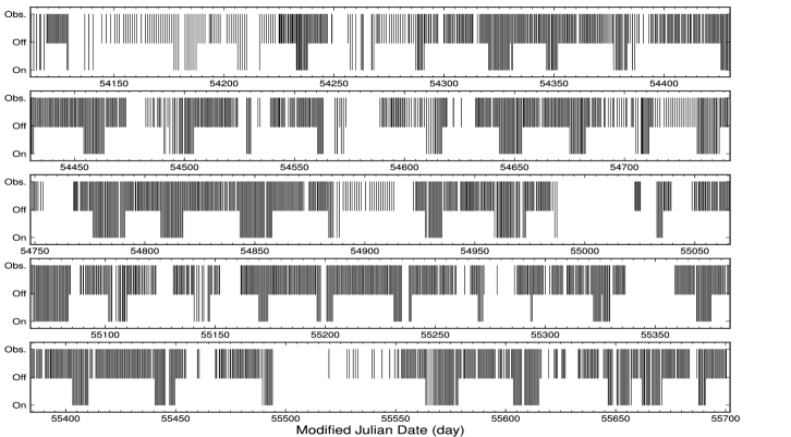
Figure 1: Sequence of observations, denoted by the black lines, carried out over $\sim 4$ yr (12 January 2007 to 19 May 2011). The data is separated into 5 contiguous 318-d panels. The times of observation and the times when PSR B1931$+$24 was radio-on (full height) and radio-off (half height) are shown by the extent of these lines.

In the data set, some of the observations which define the timescales of emission are separated by several days, particularly at earlier epochs. Therefore, a number of the inferred emission phase durations in the data do not accurately represent the behaviour of the pulsar. Consequently, we only consider emission phase durations which have gaps $\lesssim 5$ d between consecutive observations, so that we can pinpoint transition times (taken to be the midpoints between radio-on and -off observations) as accurately as possible. After applying these criteria we were left with only the highest confidence emission phase durations, which are shown in Fig. 2. We note that there is no evidence for emission cessation over timescales less than a day. The average times in each emission phase are $8\pm 4$ d and $22\pm 7$ d for the radio-on and -off phases respectively. These values are consistent with the average radio-on and -off timescales observed in Kramer et al. (2006), that is $\sim 6$ d and $\sim 28$ d respectively. We note here that the radio-on and -off timescales have a wider range of values than previously thought (Fig. 2, c.f. Fig. 1c of Kramer et al. 2006). The improvement in the determination of these values is due to the increased data span and observation cadence.

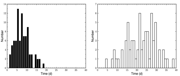
Figure 2: Histograms showing the durations when PSR B1931$+$24 is observed to be in a particular emission phase, radio-on (left) and radio-off (right).

We used these same emission phase durations to calculate the ADC; that is, the percentage of time spent in the radio-on phase, compared with the total observation time. Given that there are gaps between consecutive emission phases, and that there is a disparity between the number of suitable radio-on and -off phases, we determined the average total time spent in each emission phase through bootstrapping the observed distributions of the emission phase durations. That is, the data was sampled with replacement to obtain $10^{6}$ resamples, and average durations, for each distribution of emission phases. The resultant values were used to calculate the average ADC over the entire data-set. The error in the ADC was calculated from the uncertainty in the total time spent in the radio-on phase, which was obtained from bootstrapping the observed uncertainties. This results in an $\mathrm{ADC}=26\,\pm 6\,\%$ which is larger than, but consistent with, the Kramer et al. (2006) value of $19\pm 5\,\%$. We note that the larger uncertainty in our value most likely results from slight changes in observation cadence throughout the $\sim 13$-yr data set.

As our average ADC is the same as in Kramer et al. (2006) and yet the range of radio-on and -off durations is wider, we wanted to ascertain if there was any temporal evolution in these properties. Following the stride fitting method of Lyne et al. (2010), we determined the ADC over segments of length $T=100$ d, offset by intervals of $T/4=25$ d across the data set. We initially estimate the uncertainty in ADC for each data segment using the sum of the errors in the transition times between consecutive emission phase durations. Due to the irregular time sampling, however, there are also gaps between consecutive observations during emission phases. As the minimum time spent in a consecutive radio-on and -off phase is approximately $10$ d, we assume that any gap between a neighbouring observation which exceeds this duration should contribute to the total uncertainty in the ADC. In order to compromise between data accuracy and volume, we apply cut-offs to the uncertainties in the data; that is, we do not consider intervals which contain observations separated by more than $25$ d or whose error in the ADC is greater than $50~{}\%$. The resultant ADC as a function of time is shown in Fig. 3.

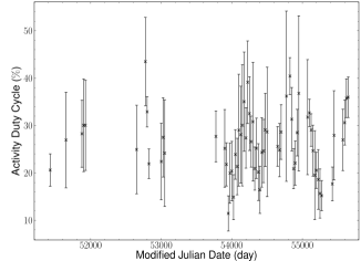
Figure 3: The evolution of the activity duty cycle of PSR B1931$+$24 over approximately 13 yr of data.

We average these values (Fig. 3) to obtain $\langle\mathrm{ADC}\rangle=26\pm 7\%$, which is consistent with that obtained by bootstrapping the emission durations. We attribute the significant error in this quantity to the notable fractional uncertainties in the ADC throughout the data set. By implementing an Anderson-Darling test (Press et al., 1992) we find that the ADC values are consistent with coming from a normal distribution, assuming Gaussian statistics for the uncertainties. There is, therefore, no compelling evidence for significant variation in the ADC of PSR B1931$+$24.

We also sought to determine whether there were any interdependencies in the characteristics of the pulsar emission. In particular, we were interested in discovering whether there is a correlation between the length of successive radio-on and -off phases. For this analysis, we selected nine data intervals from the entire data set which had the highest observation cadence and, thus, the highest confidence in emission phase durations. The properties of these data intervals are listed in Table 2. We correlated the durations of successive radio-on and -off emission phases, for each of these data intervals, to determine whether there was any connection between the length of consecutive emission phases (see Fig. 4).

Table 2: Properties of the nine data intervals chosen to characterise the correlation between the radio-on and -off emission phase durations of PSR B1931$+$24. The start and finish times of each data interval, of length $T$, are denoted by MJD_start and MJD_finish respectively. The number of emission phases which are radio-on and -off are given by $N_{\mathrm{on}}$ and $N_{\mathrm{off}}$ respectively. The average total time spent in a radio-on and -off phase are $\bar{t}_{\mathrm{on}}$ and $\bar{t}_{\mathrm{off}}$, and the activity duty cycle of the pulsar for each data interval is denoted by ADC.

MJDstart	MJDfinish	$T$ (d)	$N_{\mathrm{on}}$	$N_{\mathrm{off}}$	$\bar{t}_{\mathrm{on}}$ (d)	$\bar{t}_{\mathrm{off}}$ (d)	ADC ($\%$)
51814.07	51924.38	110.31	4	3	$7\pm 1$	$24\pm 2$	$22\pm 8$
52762.52	52921.53	159.01	5	4	$10\pm 4$	$27\pm 4$	$28\pm 2$
53733.23	53832.01	98.78	4	3	$7\pm 2$	$22\pm 7$	$29\pm 5$
53889.35	54084.26	194.91	8	7	$5\pm 1$	$21\pm 3$	$19\pm 5$
54176.30	54504.73	328.43	11	10	$9\pm 1$	$23\pm 2$	$27\pm 5$
54609.06	54743.66	134.60	5	4	$8\pm 1$	$23\pm 1$	$26\pm 4$
54775.96	54973.34	197.38	6	5	$11\pm 2$	$26\pm 4$	$30\pm 4$
55066.68	55489.50	422.82	12	12	$7\pm 1$	$28\pm 2$	$21\pm 3$
55563.29	55688.01	124.72	4	4	$12\pm 1$	$19\pm 6$	$38\pm 3$

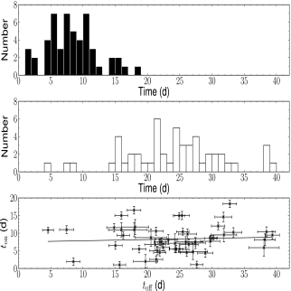
Figure 4: The correlation between the radio-on and -off emission phase durations of PSR B1931$+$24. Emission duration histograms for all the radio-on (top panel) and radio-off (middle panel) phases from the observation periods defined in Table 2, as well as the linear regression of the two parameters (bottom panel). There is no evidence for a correlation between consecutive radio-on and radio-off interval lengths.

We find that there is no significant correlation between the length of time in a given emission phase and that of the opposing mode consecutive to it. This suggests that the pulsar does not retain a memory of the length of its previous magnetospheric-state after a transition. We also computed the ADC for each data interval to determine whether the results of the previous analysis may have been biased by observation cadence (see Table 2). We again find that there is no significant evidence for variation in the ADC over time.

We were also interested in determining the average flux density of the pulsar, attributed to the different phases of emission, using the modified radiometer equation (Lorimer & Kramer, 2005):

$$S=\frac{\beta\,\textrm{SNR}\,T_{\mathrm{sys}}}{G\sqrt{n_{\mathrm{p}}\,B\,T}}\sqrt{\frac{W_{\mathrm{eq}}}{P-W_{\mathrm{eq}}}}\,.$$ (1)

Here, $\beta\sim 1$ is the digitisation factor, $G\sim 1$ Jy K^-1 is the telescope gain, $T_{\mathrm{sys}}\sim 35$ K is the average system temperature, $n_{\mathrm{p}}=2$ is the number of polarisations, $B=384$ MHz is the observing bandwidth, $P=814$ ms is the pulsar period and $W_{\mathrm{eq}}=14$ ms is the equivalent pulse width. In total, we averaged 211 radio-on and 106 radio-off DFB observations (see Fig. 5), to obtain total integration times ($T$) of approximately 40 hr and 20 hr respectively. Consequently, we place a limit on the mean flux density in the radio-off phase $S_{\mathrm{off}}\lesssim 2.0\pm 0.4~{}\mu$Jy (assuming a limiting $\mathrm{SNR}\sim 3$). For the radio-on phase, we obtain a mean flux density $S_{\mathrm{on}}=40\pm 8~{}\mu$Jy ($\mathrm{SNR}\sim 90$), which is at least 20 times brighter than that in the radio-off phase.

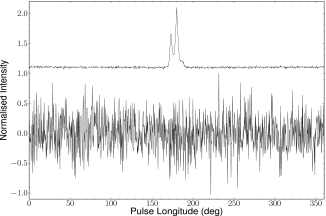
Figure 5: Average pulse profiles of PSR B1931$+$24 showing the characteristics of the radio-on (top) and radio-off emission (bottom). The peak pulse intensities are normalised to one for each emission mode profile. The radio-on profile is offset in intensity from the radio-off profile for clarity.

Converting the flux densities into pseudo-luminosities, using $L_{1400}\equiv S_{1400}\,d^{2}$ (Lorimer & Kramer, 2005), we find $L_{1400,\,\mathrm{off}}\lesssim 0.04$ mJy kpc² and $L_{1400,\,\mathrm{on}}\sim 0.84$ mJy kpc² (for a pulsar distance $d\sim 4.6$ kpc, from the NE2001 model; Cordes & Lazio 2002). We note that the upper limit on the pseudo-luminosity of PSR B1931$+$24 in the radio-off phase is barely brighter than the two weakest known radio pulsars i.e. PSR J0030+0451 ($L_{1400}\sim 0.04$ mJy kpc²; Lommen et al. 2000) and J2144$-$3933 ($L_{1400}\sim 0.02$ mJy kpc²; Lorimer 1994). This implies that the radio-off phases are consistent with emission cessation. However, it may be that the source exhibits extremely weak, underlying emission which is far below our detection threshold. This could be compared to PSR B0823$+$26, another intermittent radio source, which exhibits a factor of 100 difference in intensity between its separate emission modes (Young et al. 2012, c.f. Esamdin et al. 2005).

Observations of PSR B1931$+$24 by Kramer et al. (2006) suggest that it exhibits enhanced particle flow during its radio-on phases. We were interested in seeing whether other, less severe, changes in particle flow occurred which might also be attributed to the mechanism which determines its emission behaviour. One way to test whether the emission in these phases was consistent with a ‘steady-state’ particle flow (c.f. Crab enhanced emission, see Shearer et al. 2003), was to determine whether the pulsar exhibited any systematic pulse intensity fluctuations during radio-on phases. Such analysis is ideally performed using single-pulse data which, in this instance, was not available. Therefore, we used the 12-min average pulse profiles to determine whether there were any variations in pulse intensity, which might correlate with the position of an observation around an emission phase transition (c.f. pulse intensity decay and rise times around nulls in PSR B0809$+$74; Lyne & Ashworth 1983; van Leeuwen et al. 2002). We find that there is no significant correlation between the pulse intensity prior to, or after, a radio-off phase. We also find that there is no significant modulation in the emission during a given radio-on phase. That is, the variations in pulse intensity are dominated by random fluctuations. This suggests that the particle flow in the magnetosphere of PSR B1931$+$24 remains constant during the radio-on emission phases, to the limit of our measurement sensitivity and the intrinsic flux variation of the source.

To check whether there were any pulse shape changes during the radio-on phases, as seen in other pulsars exhibiting period derivative changes (Lyne et al., 2010), we examined the variation in the ratio of the first to second component peak intensities over time. For this analysis, we aligned DFB profiles with an analytic template using a $\chi^{2}$ minimisation method to match the pulse longitudes of the peak bins. This, in turn, enabled us to quantify the component peak intensities over time. To obtain a correct representation of the peak-to-peak ratios, we only performed this analysis on the highest SNR observations ($\textrm{SNR}>10$). Figure 6 shows the distribution of peak ratios. The average peak ratio is $0.69\pm 0.09$ and is found to be consistent with that of the analytic template (i.e. $\sim 0.7$).

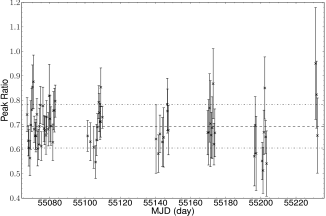
Figure 6: The evolution in the ratio of the first peak to second peak intensities of PSR B1931$+$24, over $\sim 165$ d of DFB observations. The average and $\pm 1\sigma$ values are denoted by the (dashed) and (dot-dashed) lines respectively. The fluctuation in the peak ratio values does not appear to be significant with respect to the average.

In order to determine whether the peak ratio variations were significant, we again performed an Anderson-Darling test on the distribution of values, and found no evidence to suggest the data departs from a normal distribution, assuming Gaussian error bars. As a consistency check, we also implemented a reduced $\chi^{2}$ test to quantify the fluctuations in the pulse shape. For these observations we obtain $\chi^{2}\sim 0.92$, which is consistent with random noise dominating the profile variation.

3.2 Periodicity analysis

To complement, and improve upon, the results of Kramer et al. (2006) we have conducted an extensive analysis on the periodicity of radio emission from PSR B1931$+$24, using a much longer data set (i.e. $\sim 13$ yr of data). Here, we use a modified wavelet analysis, i.e. weighted wavelet Z-statistic (WWZ) analysis (Foster, 1996; Young et al., 2012), to reveal any periodic variations within the data.

For the purpose of our analysis, we chose a wavelet tuning constant $c=0.001$ so that we could strike a balance between frequency and time resolution. The resultant WWZ transform of the one-bit time-series data, showing the evolution of the spectral power at successive epochs (or time lags), is displayed in Fig. 7. In the 2-D transform plot, we note that the peak frequencies, i.e. WWZ frequency maxima, modulate over time. This, in turn, gives rise to several features in the integrated spectrum. The broad prominent peak in the integrated spectrum shows that the WWZ power is preferentially distributed around $\sim 0.031-0.024$ d^-1 ($\sim 32-42$ d), which corresponds well with the results of Kramer et al. (2006). We also note the presence of other features in the transform plane at $\sim 0.021$ d^-1 ($\sim 48$ d), $\sim 0.035$ d^-1 ($\sim 29$ d), approximately $0.042$ d^-1 ($\sim 24$ d) and $\sim 0.052$ d^-1 ($\sim 19$ d) over small time intervals. However, they generally have much lower spectral power which casts doubt on their significance. We find that the features centred on $\sim 0.042$ d^-1 and $\sim 0.052$ d^-1 are most likely spurious due to their proximity to a long, approximately 100-d gap in the data. We note that the better observation sampling towards later times (after MJD $\sim 52810$) results in better resolution of the intrinsic variation of the source, that is the fluctuation periods are generally represented by greater WWZ power towards later times. We also consider the error estimation of these data, following Young et al. (2012), in the next subsections.

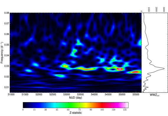
Figure 7: WWZ transform of the $\sim 13$-yr PSR B1931$+$24 radio emission activity data-set (left) and the corresponding integrated power spectrum (right). The integrated power spectrum reaches a maximum at $\sim 0.028$ d^-1 ($\sim 36$ d). Throughout the transform plane the peak frequency modulates over time, typically ranging $\sim 0.024-0.032$ d^-1 ($\sim 31-42$ d). The bootstrap $5$-$\sigma$ significance level corresponds to $Z(\omega,\tau)\approx 60$ for this data-set.

3.2.1 Confusion limit estimation method

To estimate the significance of spectral features, we first implemented the confusion limit method (see Templeton et al. 2005; Young et al. 2012). For this analysis, we located the peak fluctuation frequency (taken to be the frequency bin with the greatest spectral power) at each epoch and estimated its maximum $1$-$\sigma$ uncertainty as the half-width at half-maximum of the Z-statistic, $Z(\omega,\,\tau)$. The result of this analysis is shown in Fig. 8. We note that the peak period spans $\sim 20-50$ d over time, with a few epochs showing periodicities of $\sim 100$ d. However, the features in the wavelet transform attributed to this longer period are only represented by low WWZ power, and are over an interval of time which has a number of gaps between successive epochs ($\mathrm{MJD}\sim 51987-52034$, $\sim 52040-52077$ and $\sim 52207-52240$). Therefore, we do not believe that the longer fluctuation period is intrinsic to the source.

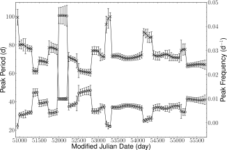
Figure 8: Peak WWZ fluctuation frequencies (crosses) and periods (open circles) for the $\sim 13$-yr PSR B1931$+$24 radio emission activity data. Error bars are $1$-$\sigma$ values computed using the confusion limit estimation method. The average error in the fluctuation frequency (or period) is approximately $6~{}\%$. Note that the peak fluctuation period spans $\sim 20-50$ d apart from at a few epochs where the data sampling is likely to have affected the local matching.

We performed another Anderson-Darling test on the peak-fluctuation period data to determine whether the variations were significant. From the results of this test, we find that the short-term modulation in the source’s periodicity (see steps in Fig. 8) is not consistent with random variation. In fact, we find that this modulation becomes more significant with increasing observation sampling. As a result, we attribute these short-term fluctuations to the quasi-periodic nature of the object.

3.2.2 Data-windowing method

As a consistency check, we also used a data-windowing method to compute a measure of the modulation in the peak frequency and period (see Young et al. 2012). Here, we split the WWZ data into 400-d segments and, for each of these segments, determined the median fluctuation frequency and corresponding period (see Table 3). These quantities were then compared with the ‘noise background’ of the WWZ data to determine their significance. Here, the noise background was estimated by computing the standard deviation of the transform data, by bootstrapping over several hundred realisations. Subsequently, we find that the first four data segments do not have median peak WWZ values greater than the $5\sigma\approx 60$ significance level derived from bootstrapping. However, the rest of the segments (excluding the data spanning $\mathrm{MJD}=54150-54550$) have values greater or equal to this cut-off, which indicate that the periodicities within these data intervals are intrinsic to the source. We note that the uncertainty in the peak fluctuation frequency becomes consistently smaller at later epochs, which results from an increase in resolution due to the improved data sampling. From this analysis, we obtain median peak fluctuation frequencies $\sim 0.035-0.021$ d^-1 ($\sim 28-47$ d), which are largely consistent with the previous analysis. Through performing another Anderson-Darling test, we find that the variations in the long-term periodicity of the source, i.e. over several years, are not significant. As a result, we infer that the overall average periodicity in the pulsar radio emission ($38\pm 5$ d) is highly stable over long timescales (i.e. years).

Table 3: Results from the data-windowing WWZ error analysis. We quote the MJD ranges of the data windows analysed, the corresponding median-peak WWZ values $\mathrm{WWZ}_{\mathrm{max}}$, as well as the peak fluctuation frequencies $\nu_{\mathrm{fluc}}$ and periods $P_{\mathrm{fluc}}$. The standard $1$-$\sigma$ uncertainties are quoted in the parentheses and are in units of the least significant digit.

MJD range	WWZmax	$\nu_{\mathrm{fluc}}$($10^{-2}$ d-1)	$P_{\mathrm{fluc}}$(d)
50950$-$51350	18 (3)	3.2 (6)	31 (6)
51350$-$51750	30 (10)	2.5 (3)	40 (5)
51750$-$52150	28 (7)	3 (1)	30 (40)
52150$-$52550	23 (4)	2.6 (7)	40 (30)
52550$-$52950	60 (20)	2.1 (4)	47 (7)
52950$-$53350	60 (20)	3.0 (7)	34 (6)
53350$-$53750	90 (10)	2.75 (4)	36 (1)
53750$-$54150	80 (30)	2.7 (3)	37 (3)
54150$-$54550	50 (20)	3.5 (5)	28 (4)
54550$-$54950	80 (30)	2.80 (5)	36 (1)
54950$-$55350	70 (30)	3.1 (2)	32 (3)
55350$-$55700	100 (20)	2.4205 (1)	41.3 (2)

3.2.3 WWZ analysis summary

The results from the WWZ analysis above show that PSR B1931$+$24 exhibits quasi-periodicity in its radio emission switching over timescales of weeks to months. That is, the source displays a relatively wide range of periodicities ($\sim 20-50$ d), when considering its short-term emission variation. Over longer timescales (i.e. years), however, the neutron star exhibits a highly stable average periodicity ($38\pm 5$ d) in its radio emission. This implies that the mechanism governing the source’s behaviour is a non-random systematic process, which is perturbed over timescales of weeks to months.

4 Spin evolution

4.1 Residual fitting and charge density estimation

To gain context on the emission modulation of PSR B1931$+$24, we studied its rotational behaviour. We were particularly interested in determining whether the object experiences any temporal evolution in the spin-down rates associated with the different phases of emission which, in turn, may be correlated with alterations to the charge density distribution of the pulsar magnetosphere (see, e.g., Timokhin 2010).

To quantify the spin-down rate variation in PSR B1931$+$24, we took a different approach compared with conventional phase-coherent timing analysis (see, e.g., Lyne et al. 1996), due to the emission cessation in this source. Kramer et al. (2006) demonstrated the success of using a dual spin-down rate, least-squares fitting method to derive the spin-parameters for this pulsar over a short span of data and, hence, the spin-down rates corresponding to each emission phase. We have expanded upon this initial analysis by applying the same fitting procedure to eight well-sampled data sets (including the one presented in Kramer et al. 2006). The procedure entails minimising the timing residuals of PSR B1931$+$24 (calculated using a fixed $\dot{\nu}$ ephemeris) by fitting for the change in rotational phase, period and period derivative ($\Delta\phi$, $\Delta P$ and $\Delta\dot{P}$ respectively) with respect to the separate emission phases. The values of $\dot{P}_{\mathrm{on},\,\mathrm{off}}$, and hence $\dot{\nu}_{\mathrm{on},\,\mathrm{off}}$, were derived from the difference between the average spin-down rate ($\dot{P}_{\mathrm{av}}$) and $\Delta\dot{P}$ associated with these modes. The total $\Delta\phi$, $\Delta P$ and $\Delta\dot{P}$, which were required to obtain a phase-coherent solution, were modelled via:

$$t_{\mathrm{res}}=\Delta\phi\cdot P+\frac{\Delta P}{P}\cdot(t-t_{\mathrm{i}})+\frac{\Delta\dot{P}_{\mathrm{i}}}{2P}\cdot(t-t_{\mathrm{i}})^{2}\,,$$ (2)

where $t_{\mathrm{res}}$ and $t_{\mathrm{i}}$ are the residual ($t_{\mathrm{obs}}-t_{\mathrm{pred}}$) and reference times respectively (here $t_{\mathrm{pred}}$ represents the time-of-arrival predicted by a single spin-down rate model), and $\Delta\dot{P}_{\mathrm{i}}$ is the change in spin-down rate in each emission phase (i.e. $\pm\Delta\dot{P}$). An example of this fitting process is shown in Fig. 9. The rotational behaviour of the pulsar is clearly characterised well by the model.

Figure 9: Least-squares, weighted fit to timing residuals of PSR B1931$+$24 for observations ranging $\mathrm{MJD}\sim 54777-54973$. The timing residuals (filled circles) here are calculated with respect to a fixed $\dot{\nu}$ ephemeris, while the fitted model (solid line) assumes two spin-down rates (see Eqn. 2).

We note that the total contribution of $\dot{\nu}_{\mathrm{on},\,\mathrm{off}}$ to the average is determined from the total time spent in a given emission phase, which is inherently dependent on the transition times between phases. Typically, we can only constrain transition times to within about a day which, in turn, imparts systematic errors into this analysis. To propagate the effects of such errors we performed a Monte-Carlo simulation on the data. Here we performed $10^{5}$ fits, for each data interval, using transition times which are randomly distributed between the last radio-on and first radio-off phase observations. As a result, we were able to obtain a distribution of radio-on and -off spin-down rates for each data interval, from which we determined estimates for their averages and associated uncertainties (see Table 4). We note that the overall average values, that is $\langle\dot{\nu}_{\mathrm{on}}\rangle=-16\pm 1\times 10^{-15}$ s^-2 and $\langle\dot{\nu}_{\mathrm{off}}\rangle=-10.8\pm 0.4\times 10^{-15}$ s^-2, are found to be consistent with Kramer et al. (2006).

Following Kramer et al. (2006), we assume that the spin-down in the radio-off states is governed by pure magnetic dipole radiation. Whereas, we assume that the spin-down in the radio-on states is supplemented by an additional torque due to an outflowing plasma (i.e. a particle wind) and its associated return current. Using this model, we can estimate the plasma charge density attributed to this wind component, to an order of magnitude, via (see Kramer et al. 2006, and references therein, for more details):

$$\rho_{\mathrm{plasma}}\approx\frac{3I\,\Delta\dot{\nu}}{R_{\mathrm{pc}}^{4}\,B_{\mathrm{s}}}\,,$$ (3)

where $I$ is the moment of inertia of the object (taken to be $10^{45}$ g cm²), $\Delta\dot{\nu}$ is the change in spin-down rate of the pulsar between emission states ($\dot{\nu}_{\mathrm{on}}-\dot{\nu}_{\mathrm{off}}$), $R_{\mathrm{pc}}=\sqrt{2\pi R^{3}\nu/c}$ is the polar cap radius of the pulsar (where the pulsar radius $R$ is taken to be $10^{6}$ cm; see, e.g., Lorimer & Kramer 2005) and the surface magnetic field strength (for the simplest case of an orthogonal rotator; see, e.g., Jackson 1962) is

$$B_{\mathrm{s}}\sim 3.2\times 10^{19}\,\sqrt{\left(\frac{-\dot{\nu}_{\mathrm{off}}}{1\,\rm{s}^{-2}}\right)\!\left(\frac{\nu}{1\,\rm{s}^{-1}}\right)^{\!-3}}\,\rm{Gauss}\,.$$ (4)

By substituting $R_{\mathrm{pc}}$ and $B_{\mathrm{s}}$ into Eqn. 3, $\rho_{\mathrm{plasma}}$ was directly calculated for each data interval via:

$$\rho_{\mathrm{plasma}}\sim 7.1\times 10^{5}\!\left(\frac{\Delta\dot{\nu}}{1\,\rm{s}^{-2}}\right)\!\!\left(\frac{1\,\rm{s}^{-1}}{\nu}\right)^{\!\!1/2}\!\!\left(\frac{1\,\rm{s}^{-2}}{\dot{\nu}_{\mathrm{off}}}\right)^{\!\!1/2}\!\rm{C}\,\rm{m}^{-3}.$$ (5)

These quantities were also compared with the Goldreich-Julian charge density of the object, which was estimated, to an order of magnitude, by (see, e.g., Lorimer & Kramer 2005):

$$\rho_{{}_{\mathrm{GJ}}}=\frac{B_{\mathrm{s}}\,\nu}{c}\sim 3.6\times 10^{5}\left(\frac{\dot{\nu}_{\mathrm{off}}}{1\,\rm{s}^{-2}}\right)^{\!\!1/2}\!\!\left(\frac{1\,\rm{s}^{-1}}{\nu}\right)^{\!\!1/2}\mathrm{C}\,\mathrm{m}^{-3}.$$ (6)

Using the average values for $\dot{\nu}_{\mathrm{off}}=-10.8\pm 0.4\times 10^{-15}$ s^-2 and $\nu=1.228965\pm 0.000001$ Hz, obtained from the fitting process, we estimate $\rho_{{}_{\mathrm{GJ}}}$ to be approximately $0.033\,\rm{C}\,\rm{m}^{-3}$. Table 4 shows the results of this analysis. We note that different values are measured for $\dot{\nu}_{\mathrm{on}}$ and $\dot{\nu}_{\mathrm{off}}$ over neighbouring data intervals. However, given the uncertainties in these parameters, we consider the different spin-down rates for each emission phase to be consistent with the overall averages of $\dot{\nu}_{\mathrm{on}}$ and $\dot{\nu}_{\mathrm{off}}$. This is supported by the results of an Anderson-Darling test, from which we conclude that the distributions of $\dot{\nu}_{\mathrm{on}}$ and $\dot{\nu}_{\mathrm{off}}$ follow Gaussian statistics. As a result, we do not consider the variations in $\rho_{\mathrm{plasma}}$ with respect to $\rho_{{}_{\mathrm{GJ}}}$ to be significant.

Table 4: Summary of the results from the residual fitting analysis. The epoch of the spin parameters for each fit is denoted by $\mathrm{Pepoch}$, $T$ is the length of each fit interval and $\dot{\nu}_{\mathrm{on}}$, $\dot{\nu}_{\mathrm{off}}$ are the radio-on and radio-off spin-down rates respectively. The change in spin-down rate (i.e. $\dot{\nu}_{\mathrm{on}}-\dot{\nu}_{\mathrm{off}}$) is represented by $\Delta\dot{\nu}$. Definitions for $\rho_{{}_{\mathrm{GJ}}}$ and $\rho_{\mathrm{plasma}}$ can be found in the text. Standard $1$-$\sigma$ errors are provided in the parentheses, after the parameters (where possible), and represent the least significant digit.

$\mathrm{Pepoch}$	$T$ (d)	$\dot{\nu}_{\mathrm{on}}$ ($10^{-15}$ s-2)	$\dot{\nu}_{\mathrm{off}}$ ($10^{-15}$ s-2)	$\Delta\dot{\nu}/\dot{\nu}_{\mathrm{av}}$ ($\%$)	$\rho_{\mathrm{plasma}}$ ($10^{-2}$ Cm-3)	$\rho_{\mathrm{plasma}}/\rho_{{}_{\mathrm{GJ}}}$ ($\%$)
51869.7	107.5	-15.2 (2)	-11.13 (9)	36.6 (6)	2.5	73
52842.3∗	157.5	-16.0 (2)	-10.78 (7)	48.4 (7)	3.2	96
53782.6	97.7	-17.6 (5)	-10.4 (2)	69 (2)	4.5	134
53987.1	193.4	-19 (1)	-10.2 (2)	83 (5)	5.4	160
54340.7	326.8	-16.2 (4)	-10.7 (1)	51 (1)	3.4	102
54676.6	133.0	-17.1 (8)	-10.3 (3)	66 (4)	4.3	130
54875.0	196.0	-15.8 (2)	-11.07 (8)	42.7 (6)	2.9	87
55198.2	262.2	-14.3 (1)	-11.40 (3)	25.4 (2)	1.7	52

${}^{*}\mathrm{Pepoch}$ of data used to derive spin-parameters in Kramer et al. (2006).

4.2 Measurement of the braking index

In the radio-off phase, the rotational slow-down of the pulsar $\dot{\nu}_{\mathrm{off}}$ is thought to be indicative of the torque produced by magneto-dipole radiation (Kramer et al., 2006). Consequently, the rate of change in the spin-down rate in the radio-off phase $\ddot{\nu}_{\mathrm{off}}$ should provide a measure of the braking index associated with this radiation (e.g. Taylor & Manchester 1977)

$$n=\frac{\nu\ddot{\nu}_{\mathrm{off}}}{\dot{\nu}^{2}}\,,$$ (7)

which is not contaminated by the additional electromagnetic torque of the plasma current flow; that is, assuming that the additional torque completely disappears in the radio-off phase. This is particularly important as measurement of this parameter can offer significant information about how the pulsar undergoes its energy loss and, ultimately, provide us with insight into the electrodynamics (see, e.g., Xu & Qiao 2001; Wu et al. 2003; Ruderman 2005; Contopoulos 2007).

Here, we fitted the derived values for $\dot{\nu}_{\mathrm{on}}$ and $\dot{\nu}_{\mathrm{off}}$ for a number of epochs to determine if significant second order variations could be measured (Fig. 10). Unfortunately, however, we could not obtain a significant value for $\ddot{\nu}_{\mathrm{off}}$ using data even with the greatest observation density (Table 5, see also $\S$5 for a discussion on this). As a result, we could not obtain an accurate measure of the braking index of the source.

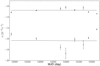
Figure 10: Linear regression fits of $\dot{\nu}_{\mathrm{off}}$ (top trace) and $\dot{\nu}_{\mathrm{on}}$ (bottom trace) for PSR B1931$+$24. Note the anti-correlation in the data, which affects the quality of the fits (see text for details).

Table 5: The results of the linear regression analysis of the spin-down rate data, with least significant uncertainties in the parentheses. The length of each fitted data-set is denoted by $T$. The correlation coefficient and two-sided probability value for each fit are given by $R$ and $p$ respectively. The rate of change in the spin-down rate is represented by $\ddot{\nu}_{\mathrm{off}}$, with the associated $1$-$\sigma$ error quoted in the parentheses (in units of the least significant digit).

$T$ (d)	$R$	$p$	$\ddot{\nu}_{\mathrm{off}}$ ($10^{-19}$ s-3)
3328.5	0.01	0.97	0.05 (156)
2355.9	-0.42	0.35	-2 (2)
1415.5	-0.78	0.06	-7 (3)

Consequently, we sought to determine a value for braking index using another method. Using the timing software developed by Weltevrede et al. (2011), we also modelled the variation in spin-down rate in PSR B1931$+$24, by fitting changes in rotational phase to the times-of-arrival (using the first three terms of Eqn. 7 in Weltevrede et al. 2011). These changes in rotational phase are analogous to glitches, that is they are discrete changes in spin-down rate, although there are no jumps in spin frequency. In our model, each emission phase has a unique spin-down rate (i.e. there is only one value for $\dot{\nu}_{\mathrm{on}}$ and $\dot{\nu}_{\mathrm{off}}$), which we assume is acquired directly after (or before) the last (or first) radio-on observation of each active emission phase. Through fitting the observed times-of-arrival for changes in spin-down rate only, we find that this method produces results consistent with Table 4. However, when the emission phase transition times are also taken as a fit parameter we obtain very poor fits. We applied maximum and minimum time constraints to the ‘glitch epochs’ but, due to the absence of data bounding a given transition into (or out of) a radio-on phase, the fitting process could not converge; a global solution could not be achieved because times-of-arrival are limited to the radio-on phase data.

4.3 Long-term evolution in spin-down rate

Using the results from the residual fitting in $\S$4.1, we were unable to determine a significant value for $\ddot{\nu}_{\mathrm{off}}$ or $n$ for the pulsar. This is most likely due to the transition time errors, between emission phases, which introduce an anti-correlation between $\dot{\nu}_{\mathrm{on}}$ and $\dot{\nu}_{\mathrm{off}}$ (a linear fit to these data obtains a correlation coefficient $R=-0.9$ and two-sided p-value $p=0.0003$; see also Fig. 10). That is, systematic over- and under-estimation of the transition times, which are not fitted for, cause $\dot{\nu}_{\mathrm{on}}$ and $\dot{\nu}_{\mathrm{off}}$ to become anti-correlated which, in turn, increases the noise contribution to $\ddot{\nu}_{\mathrm{off}}$.

To complement this analysis, therefore, we decided to examine the long-term evolution in the spin-down rates over the entire $\sim 13$-yr data-set. For this analysis, we used timing measurements of PSR B1931$+$24 to estimate the contribution of $\dot{\nu}_{\mathrm{on}}$ to the rotational frequency $\nu$ over neighbouring radio-on phases. We assumed that the change in rotational frequency $\Delta\nu$, resulting from variation between $\dot{\nu}_{\mathrm{on}}$ and $\dot{\nu}_{\mathrm{off}}$, can be obtained from fitting the residuals of three successive radio-on phases in separate pairs (see Fig. 11). In order to separate the effects of the different spin-down rates in these fits, we first form residuals by using a fixed $\dot{\nu}$, set to be the average $\dot{\nu}_{\mathrm{off}}$ (using the average determined from residual fitting, i.e. $\langle\dot{\nu}_{\mathrm{off}}\rangle=-10.8\pm 0.4\times 10^{-15}$ s^-2). We fitted the timing residuals of the latter and first halves of a given pair of radio-on phases, using PSRTIME, to estimate a value for the rotational frequency which is governed by the radio-off spin-down rate. We assumed that the contribution of $\dot{\nu}_{\mathrm{on}}$ to these residuals was negligible due to the short length of time the radio-on phases cover (w.r.t. the radio-off phases). By obtaining values for $\nu$, for the first and second pair of radio-on phases, we were able to estimate the total change in rotational frequency due to the difference in spin-down rate $\Delta\dot{\nu}$ over the central radio-on phase. Given that $\dot{\nu}_{\mathrm{on}}$ should only affect the residuals over this period, we obtain the relation

$$\Delta\nu=\nu_{23}-\nu_{12}=\Delta\dot{\nu}\times t_{\mathrm{on}}\,,$$ (8)

where $\Delta\dot{\nu}$ represents $\dot{\nu}_{\mathrm{on}}-\dot{\nu}_{\mathrm{off}}$ and $t_{\mathrm{on}}$ is the total time spent in the central radio-on phase. The spin-frequencies for the first and second fit intervals are $\nu_{12}$ and $\nu_{23}$ respectively, as shown in Fig. 11.

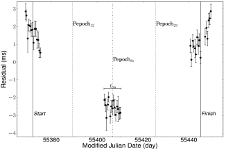
Figure 11: Timing residuals of PSR B1931$+$24, over approximately $80$ d of data, depicting the $\Delta\nu$ fitting process. The epochs where $\nu$ was calculated are represented by $\textrm{Pepoch}_{\,12}$ and $\textrm{Pepoch}_{\,23}$ for the first and second pair of radio-on phases respectively. The epoch at which $\Delta\nu$, hence $\Delta\dot{\nu}$, was measured is denoted by $\textrm{Pepoch}_{\,\mathrm{fit}}$. The bounding regions of the fits are shown by the ‘start’ and ‘finish’ lines.

To increase the number of measurements, we analysed the data using a stride-fitting method similar to that used by Lyne et al. (2010); we analysed groups of radio-on phase data in steps of single emission phases. We only included data windows which had three well defined radio-on phases i.e. containing gaps no greater than $10$ d between observations, with uncertainties in the emission phase transitions less than $4$ d (less than $2$ d for the longest data-set; see Table 6). We corrected for the long-term spin-down behaviour of the source by subtracting the average spin-down rate from the frequency data using the vfit program.

Noting that Eqn. 8 is analogous to the equation for a straight-line, with a gradient equal to $\Delta\dot{\nu}$ and zero intercept, we were able to fit $\Delta\nu$ vs $t_{\mathrm{on}}$ across numerous data intervals, as shown in Fig. 12 and Table 6. We find that these data are highly linearly correlated, which suggests that $\dot{\nu}_{\mathrm{on}}$ and $\dot{\nu}_{\mathrm{off}}$ are well defined. We find that there is no evidence for variation in the spin-down rates associated with the different phases of emission within our measurement sensitivity.

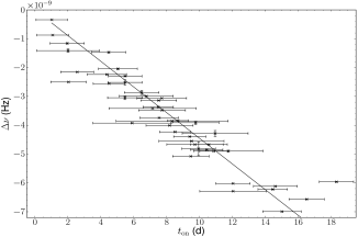
Figure 12: A linear fit to the change in rotational frequency ($\Delta\nu$) against radio-on phase length ($t_{\mathrm{on}}$) for approximately 13 yr of observations of PSR B1931$+$24.

Table 6: The linear fit parameters for the long-term spin-down rate study of PSR B1931$+$24. The MJD mid-point of each data-set used is denoted by $\mathrm{MJD}_{\mathrm{mid}}$. The total length of each data-set is represented by $T$ and $N$ is the number of data points used in each fit. The change in spin-down rate obtained from the fitting procedure is denoted by $\Delta\dot{\nu}$ and $\dot{\nu}_{\mathrm{on}}$ is the corresponding radio-on spin-down rate. Standard ($1$-$\sigma$) errors for $\Delta\dot{\nu}$ and $\dot{\nu}_{\mathrm{on}}$ are provided in parentheses after the parameters, and represent the least significant digit.

$\mathrm{MJD}_{\mathrm{mid}}$	$T$ (d)	$N$	$\Delta\dot{\nu}$ ($10^{-15}$ s-2)	$\dot{\nu}_{\mathrm{on}}$ ($10^{-15}$ s-2)
51646.0	1426	8	-5.6 (8)	-16 (1)
53143.4	1451	9	-4 (1)	-16 (1)
54602.8	1467	29	-5.2 (3)	-16.0 (5)
53356.2	4688	45	-5.2 (2)	-16.0 (4)

5 Discussion

We have shown that PSR B1931$+$24 exhibits regulated emission modulation; that is, to the limit of our measurements it maintains a constant ADC. To improve on these results, even more frequent sampling would be required. This would only be feasible with a large dedicated telescope, or new facilities such as LOFAR and the SKA which will have multi-beam capabilities and, hence, greater ability to dedicate observing time to individual sources. If we were to observe this source over hourly timescales, rather than daily, we would dramatically increase our chances of observing the pulsar transition between emission modes. As a result, we would possibly be able to uncover correlated changes in emission following (or preceding) radio-off phases which might give us insight into what causes the magnetospheric configuration to change so dramatically.

We also characterised the modulation timescales of the radio emission in PSR B1931$+$24. We find that the source exhibits a periodic modulation timescale of approximately 38 d on average. There do appear to be variations around this basic periodicity, but it remains remarkably stable over many years. This degree of stability provides a challenge for models of this process as it is significantly longer than the expected dynamic and plasma timescales ($\sim$ ms; e.g. Ruderman & Sutherland 1975).

Using a residual fitting method, we find that the variations in $\dot{\nu}_{\mathrm{on}}$ and $\dot{\nu}_{\mathrm{off}}$, throughout the $\sim 13$-yr data set, are consistent with the measurement uncertainties (see $\S$ 4.1). This result is supported by the long-term analysis (see $\S$ 4.3), which provides additional evidence to suggest that we do not observe any significant changes in the spin-down rates attributed to each emission mode; that is, the pulsar appears to retain a constant $\Delta\dot{\nu}=48\pm 2\%$ between emission phases. This implies that the apparent changes in plasma flow in the radio-on phase are also not significant ($\langle\rho_{\mathrm{plasma}}\rangle=4\pm 1\times 10^{-2}$ Cm^-3; see Table 4), thus indicating a surprisingly high degree of stability in the bi-modal system.

We note, however, that there is an unavoidable systematic effect in the short-timescale fitting procedure. More specifically, the errors in the transition times between emission phases introduced uncertainty into the calculation of $\dot{\nu}_{\mathrm{on}}$ and $\dot{\nu}_{\mathrm{off}}$. This is highlighted by the results in Fig. 10, where the interdependency between the two spin parameters is made evident. We see that these quantities are in fact almost perfectly anti-correlated. In our model, the transition times between phases of emission are not taken as a fit parameter. Therefore, observations spaced farther apart between two emission modes will have a higher uncertainty in the transition time compared with two spaced closer together. Furthermore, if the amount of time spent in a radio-on phase is overestimated, then the amount of time in a consecutive radio-off phase will be underestimated accordingly. Given that radio-on phases are much shorter than radio-off phases on average, it is evident that the effect on the error of $\dot{\nu}_{\mathrm{on}}$ will be greater than that of $\dot{\nu}_{\mathrm{off}}$. This naturally explains the observed anti-correlation between the two parameters and the larger error bars in $\dot{\nu}_{\mathrm{on}}$. Therefore, it is possible that we did not see any significant variation in the spin-down rates due to this systematic effect. To overcome this problem, we again would require greater observation cadence to provide better constraints on the transition times.

We also attempted to obtain a value for the braking index of PSR B1931$+$24 from $\ddot{\nu}_{\mathrm{off}}$, in the hope of determining information about the energy loss of the object. Using Eqn. 7, we predicted the $\ddot{\nu}$ that would be required to obtain a braking index $n=3$. Assuming the average parameters for $\nu$ and $\dot{\nu}_{\mathrm{off}}$ from residual fitting, we would expect $\ddot{\nu}=2.85\pm 0.05\times 10^{-28}$ s ^-3 (i.e. $\sim 10^{9}$ less than the upper limit derived from fitting separate residual data-sets). Given the level of timing noise in this pulsar, and the $\ddot{\nu}$ quoted in Hobbs et al. (2010), it seems very improbable that any increase in data density would allow us to obtain a value for $\ddot{\nu}$ as low as that predicted from theory. The problem lies in decoupling the long-term contribution of $\dot{\nu}_{\mathrm{on}}$ from the timing residuals; that is, the value for $\ddot{\nu}$ from global fitting will always be contaminated by the modulation of $\dot{\nu}$. In the case of local fitting ($\dot{\nu}_{\mathrm{on},\,\mathrm{off}}$), there will probably always be an uncertainty in the transition times which, again, means that it will be difficult to decouple $\dot{\nu}_{\mathrm{on},\,\mathrm{off}}$ from $\dot{\nu}_{\mathrm{av}}$.

With the next generation of telescopes (e.g. LOFAR, FAST, ASKAP, MeerKAT and the SKA) coming online in the near future, we anticipate a dramatic increase in the number of known intermittent pulsars. Coupled with the continued observation of known intermittent sources (e.g. PSRs B0823$+$26, J1832$+$0029, J1841$-$0500 and B1931$+$24), characterisation of these objects should lead to an improved understanding of the general emission and rotational properties of pulsars which, ultimately, should facilitate the development of more realistic radio emission and magnetospheric models. These observations should also provide further insight into how the different ‘types’ of nulling pulsars, i.e. normal nulling pulsars, RRATs and longer-term intermittent pulsars, are related.

6 Conclusions

In this work, we have confirmed and expanded substantially upon the findings of Kramer et al. (2006), which has enabled us to provide further evidence for the magnetospheric-state switching scenario (e.g. Bartel et al. 1982; Lyne et al. 2010; Timokhin 2010). In order to determine how these events are triggered (e.g. via ‘circumpulsar asteroids’; Cordes & Shannon 2008), however, it is clear that dedicated infra-red and high-energy observations of this source are required.

If the spin-down rates attributed to each emission mode, and ADC, for this pulsar are truly constant over time, as suggested by our observations, this would be quite remarkable; as of yet, there is no clear reason to suggest why a pulsar should retain a memory of its previous magnetospheric state i.e. particle flow (c.f. Li et al. 2012). This raises a couple of important questions: 1) Is there charge or matter transfer in the magnetosphere which leads to these separate regulated states and, if so, how would this occur? 2) Why does the pulsar consistently assume the same rotational and emission characteristics? These questions are likely only to be answered based on future observations of this source and others like it, which may as yet be undiscovered. We note, however, that the rate at which new intermittent sources sources are discovered should increase significantly with the use of next generation telescopes. Therefore, we may only need to wait a few years before significant breakthrough is made in magnetospheric modelling and our understanding of emission cessation in pulsars.

7 Acknowledgements

We thank D. J. Champion and M. D Gray for useful discussion which has contributed to this paper. We are grateful to C. Jordan, and the several telescope operators at Jodrell Bank, for obtaining the majority of the data used in this work. NJY acknowledges support from the National Research Foundation (NRF). The Nançay Radio Observatory is operated by the Paris Observatory, associated with the French Centre National de la Reserche Scientifique (CNRS).

References

- Backer (1970) Backer D. C., 1970, Nature, 228, 42
- Bartel et al. (1982) Bartel N., Morris D., Sieber W., Hankins T. H., 1982, ApJ, 258, 776
- Camilo et al. (2012) Camilo F., Ransom S. M., Chatterjee S., Johnston S., Demorest P., 2012, ApJ, 746, 63
- Contopoulos (2005) Contopoulos I., 2005, A&A, 442, 579
- Contopoulos (2007) Contopoulos I., 2007, A&A, 466, 301
- Cordes & Lazio (2002) Cordes J. M., Lazio T. J. W., 2002, arXiv:astro-ph/0207156
- Cordes & Shannon (2008) Cordes J. M., Shannon R. M., 2008, ApJ, 682, 1152
- Esamdin et al. (2005) Esamdin A., Lyne A. G., Graham-Smith F., Kramer M., Manchester R. N., Wu X., 2005, MNRAS, 356, 59
- Foster (1996) Foster G., 1996, Astron. J., 112, 1709
- Geppert et al. (2003) Geppert U., Rheinhardt M., Gil J., 2003, A&A, 412, L33
- Hobbs et al. (2010) Hobbs G., Lyne A. G., Kramer M., 2010, MNRAS, 402, 1027
- Jackson (1962) Jackson J. D., 1962, Classical Electrodynamics. Wiley
- Jones (2012) Jones D. I., 2012, MNRAS, 420, 2325
- Kramer et al. (2006) Kramer M., Lyne A. G., O’Brien J. T., Jordan C. A., Lorimer D. R., 2006, Science, 312, 549
- Li et al. (2012) Li J., Spitkovsky A., Tchekhovskoy A., 2012, ApJL, 746, L24
- Lommen et al. (2000) Lommen A. N., Zepka A., Backer D. C., McLaughlin M., Cordes J. M., Arzoumanian Z., Xilouris K., 2000, ApJ, 545, 1007
- Lorimer (1994) Lorimer D. R., 1994, PhD thesis, The University of Manchester
- Lorimer & Kramer (2005) Lorimer D. R., Kramer M., 2005, Handbook of Pulsar Astronomy. Cambridge University Press
- Lorimer et al. (2012) Lorimer D. R., Lyne A. G., McLaughlin M. A., Kramer M., Pavlov G. G., Chang C., 2012, ApJ, 758, 141
- Lyne et al. (2010) Lyne A., Hobbs G., Kramer M., Stairs I., Stappers B., 2010, Science, 329, 408
- Lyne & Ashworth (1983) Lyne A. G., Ashworth M., 1983, MNRAS, 204, 519
- Lyne et al. (1996) Lyne A. G., Pritchard R. S., Graham-Smith F., Camilo F., 1996, Nature, 381, 497
- McLaughlin et al. (2006) McLaughlin M. A., Lyne A. G., Lorimer D. R., Kramer M., Faulkner A. J., Manchester R. N., Cordes J. M., Camilo F., Possenti A., Stairs I. H., Hobbs G., D’Amico N., Burgay M., O’Brien J. T., 2006, Nature, 439, 817
- Press et al. (1992) Press W. H., Teukolsky S. A., Vetterling W. T., Flannery B. P., 1992, Numerical Recipes: The Art of Scientific Computing, 2nd edition. Cambridge University Press, Cambridge
- Rankin (1986) Rankin J. M., 1986, ApJ, 301, 901
- Rea et al. (2008) Rea N., Kramer M., Stella L., Jonker P. G., Bassa C. G., Groot P. J., Israel G. L., Méndez M., Possenti A., Lyne A., 2008, MNRAS, 391, 663
- Rheinhardt et al. (2004) Rheinhardt M., Konenkov D., Geppert U., 2004, A&A, 420, 631
- Ritchings (1976) Ritchings R. T., 1976, MNRAS, 176, 249
- Rosen et al. (2011) Rosen R., McLaughlin M. A., Thompson S. E., 2011, ApJL, 728, L19
- Ruderman (2005) Ruderman M., 2005, ArXiv Astrophysics e-prints
- Ruderman & Sutherland (1975) Ruderman M. A., Sutherland P. G., 1975, ApJ, 196, 51
- Shearer et al. (2003) Shearer A., Stappers B., O’Connor P., Golden A., Strom R., Redfern M., Ryan O., 2003, Science, 301, 493
- Stokes et al. (1985) Stokes G. H., Taylor J. H., Weisberg J. M., Dewey R. J., 1985, Nature, 317, 787
- Taylor & Manchester (1977) Taylor J. H., Manchester R. N., 1977, ApJ, 215, 885
- Templeton et al. (2005) Templeton M. R., Mattei J. A., Willson L. A., 2005, AJ, 130, 776
- Timokhin (2010) Timokhin A. N., 2010, MNRAS, 408, L41
- Urpin & Gil (2004) Urpin V., Gil J., 2004, A&A, 415, 305
- van Leeuwen et al. (2002) van Leeuwen A. G. J., Kouwenhoven M. L. A., Ramachandran R., Rankin J. M., Stappers B. W., 2002, A&A, 387, 169
- van Leeuwen & Stappers (2010) van Leeuwen J., Stappers B. W., 2010, A&A, 509, A7
- Wang et al. (2007) Wang N., Manchester R. N., Johnston S., 2007, MNRAS, 377, 1383
- Weltevrede et al. (2011) Weltevrede P., Johnston S., Espinoza C. M., 2011, MNRAS, 411, 1917
- Wu et al. (2003) Wu F., Xu R. X., Gil J., 2003, A&A, 409, 641
- Xu & Qiao (2001) Xu R. X., Qiao G. J., 2001, ApJL, 561, L85
- Young et al. (2012) Young N. J., Stappers B. W., Weltevrede P., Lyne A. G., Kramer M., 2012, MNRAS, 427, 114
- Zhang et al. (1997) Zhang B., Qiao G. J., Lin W. P., Han J. L., 1997, ApJ, 478, 313