Convergent finite difference methods for one-dimensional fully nonlinear second order partial differential equations

Abstract

This paper develops a new framework for designing and analyzing convergent finite difference methods for approximating both classical and viscosity solutions of second order fully nonlinear partial differential equations (PDEs) in 1-D. The goal of the paper is to extend the successful framework of monotone, consistent, and stable finite difference methods for first order fully nonlinear Hamilton-Jacobi equations to second order fully nonlinear PDEs such as Monge-Ampère and Bellman type equations. New concepts of consistency, generalized monotonicity, and stability are introduced; among them, the generalized monotonicity and consistency, which are easier to verify in practice, are natural extensions of the corresponding notions of finite difference methods for first order fully nonlinear Hamilton-Jacobi equations. The main component of the proposed framework is the concept of a “numerical operator”, and the main idea used to design consistent, generalized monotone and stable finite difference methods is the concept of a “numerical moment”. These two new concepts play the same roles the “numerical Hamiltonian” and the “numerical viscosity” play in the finite difference framework for first order fully nonlinear Hamilton-Jacobi equations. In the paper, two classes of consistent and monotone finite difference methods are proposed for second order fully nonlinear PDEs. The first class contains Lax-Friedrichs-like methods which also are proved to be stable, and the second class contains Godunov-like methods. Numerical results are also presented to gauge the performance of the proposed finite difference methods and to validate the theoretical results of the paper.

1 Introduction

Fully nonlinear partial differential equations (PDEs) refers to a class of nonlinear PDEs which are nonlinear in the highest order derivatives of the unknown functions appearing in the equations. For example, the general first and second order fully nonlinear PDEs, respectively, have the form $H(\nabla u,u,x)=0$ and $F(D^{2}u,\nabla u,u,x)=0$, where $\nabla u$ and $D^{2}u$ denote the gradient vector and Hessian matrix of the unknown function $u$. Fully nonlinear PDEs, which have experienced extensive analytical developments in the past thirty years (cf. [4, 1, 11, 18]), arise from many scientific and engineering applications such as differential geometry, astrophysics, antenna design, image processing, optimal control, optimal mass transport, and geostrophical fluid dynamics. Fully nonlinear PDEs play a critical role for the solutions of these applications because they appear one way or another in the governing equations of these problems.

As expected, the study of first order fully nonlinear PDEs came first. Since the introduction of the notion of viscosity solutions by Crandall and Lions [6] in 1983, the past thirty years has been a period of explosive developments in analyzing first order fully nonlinear PDEs. Starting with the pioneering work of Crandall and Lions [7], extensive research has also been successfully carried out on developing numerical methods, in particular monotone as well as other types of finite difference methods, for computing viscosity solutions of first order fully nonlinear PDEs, especially those arising from the level set formulations of moving interfaces and those arising from optimal control (cf. [20] and the references therein). To overcome the low order accuracy barrier of monotone finite difference methods, various high order local discontinuous Galerkin (LDG) methods have also been developed recently in the literature (cf. [20, 21] and the references therein).

In contrast with the success of PDE analysis and numerical approximation for first order fully nonlinear PDEs, the situation for second order fully nonlinear PDEs is very different. On one hand, like in the case of first order fully nonlinear PDEs, tremendous progresses in PDE analysis have been made in the past thirty years (cf. [11, 4]). On the other hand, not much progress on developing accurate and efficient numerical methods, especially Galerkin-type methods, for second order fully nonlinear PDEs has been made until very recently (cf. [13, 14] and the references therein). The lack of progress is mainly due to the following two facts: (i) the notion of viscosity solutions is nonvariational; (ii) the conditional uniqueness (i.e., uniqueness only holds in a restrictive function class) of viscosity solutions is difficult to handle at the discrete level. The first difficulty prevents a direct construction of Galerkin-type methods and forces one to use indirect approaches as done in [9, 10, 12, 14] for approximating viscosity solutions. The second difficulty prevents any straightforward construction of finite difference methods because such a method does not have a mechanism to enforce the conditional uniqueness and often fails to capture the sought-after viscosity solution. Since the scope of this paper is confined to the finite difference method, Galerkin-type methods will not be discussed here. We refer the reader to the review paper [13] for a detailed discussion of recent developments on Galerkin-type methods for second order fully nonlinear PDEs.

The primary goal of this paper is to develop a new framework for designing and analyzing convergent finite difference methods for second order fully nonlinear (elliptic) PDEs. For the ease of presenting the ideas and to observe the page limitation of the journal, we shall only consider one-dimensional PDEs in this paper and leave the high dimensional generalizations to a forthcoming companion paper [15]. We use the phrase “new framework” to distinguish the framework of this paper from the existing (abstract) framework originally developed by Barles and Souganidis in [2] twenty years ago and further developed recently by Caffarelli and Souganidis in [5]. Unlike Barles and Souganidis’ framework which is abstract and broader in applications, our framework is specifically and only designed for finite difference methods which can be easily implemented on computers. As a result, the proposed framework has the advantages of being simple to understand and easy to utilize in practice. Moreover, the new framework is a natural extension of the successful monotone finite difference framework developed for first order fully nonlinear Hamilton-Jacobi equations (cf. [7, 20] and the references therein). The main concept of the new framework is the “numerical operator”. The key components of the framework are new and easy-to-check notions of consistency and generalized monotonicity (g-monotonicity), which together with the well-known notion of stability, form the backbones of the proposed finite difference framework. After the framework is established, one must address a harder question of how to construct specific finite difference methods which fulfill the structure conditions (i.e., consistency, g-monotonicity, and stability) of the framework in order to make the framework practically useful. We note that this question was not addressed in [2] as the goal of that paper was not to develop practical numerical methods, and it took seventeen years to construct the first finite difference method which fulfills the structure conditions laid out in [2] for the second order fully nonlinear Monge-Ampère equation in [19]. Moreover, the method of [19] is a nonstandard finite difference method because it requires the use of wide-stencil grids. We do want to remark that many numerical methods, which may or may not fulfill the structure conditions of [2], have been developed for Bellman type equations (cf. [3, 16, 13] and the references therein). To address the above key question, our main idea is to introduce a new concept called the “numerical moment”. We like to stress that the numerical moment not only helps the construction of desired g-monotone finite difference methods, but also, we believe, provides a fundamental and indispensable mechanism for a finite difference method to overcome the two major difficulties associated with numerical approximations of second order fully nonlinear PDEs. We also note that the new concepts of “numerical operators” and “numerical moments” for second order fully nonlinear PDEs are natural extensions of the well-known concepts of “numerical Hamiltonians” and “numerical viscosities” for first order fully nonlinear Hamilton-Jacobi equations.

This paper is organized as follows. In Section 2 we collect some preliminary materials such as notation and definitions. In Section 3 we present our finite difference framework. The motivation and main ideas are heuristically explained. The main concepts and definitions of numerical operators, consistency, g-monotonicity, and stability are formally introduced and defined. The main result of this section is a convergence theorem which asserts that the solution of any consistent, g-monotone and stable finite difference method is guaranteed to converge to the unique viscosity solution of the underlying second order fully nonlinear PDE. In Section 4 we introduce the concept of a numerical moment. With the help of the numerical moment and the inspiration given by the convergent finite difference schemes for first order fully nonlinear Hamilton-Jacobi equations, we are able to construct two classes of consistent and g-monotone finite difference methods. The first class contains Lax-Friedrichs-like methods and the second class contains Godunov-like methods. By using a non-standard fixed point argument we also prove that every consistent and g-monotone Lax-Friedrichs-like method is uniquely solvable and stable for a given class of fully nonlinear operators. In Section 5 we present some detailed numerical results to gauge the performance of the proposed finite difference methods and to validate the theoretical results of the paper. The paper is concluded by a short summary in Section 6.

2 Preliminaries

In this paper we adopt standard function and space notations as in [11, 4]. For example, for a bounded open domain $\Omega\subset\mathbf{R}^{d}$, $B(\Omega)$, $USC(\Omega)$ and $LSC(\Omega)$ are used to denote, respectively, the spaces of bounded, upper semi-continuous and lower semicontinuous functions on $\Omega$. Also, for any $v\in B(\Omega)$, we define

$$v^{*}(x):=\limsup_{y\to x}v(y)\qquad\mbox{and}\qquad v_{*}(x):=\liminf_{y\to x}v(y).$$

Then, $v^{*}\in USC(\Omega)$ and $v_{*}\in LSC(\Omega)$, and they are called the upper and lower semicontinuous envelopes of $v$, respectively.

Given a bounded function $F:\mathcal{S}^{d\times d}\times\mathbf{R}^{d}\times\mathbf{R}\times\overline{\Omega}\to\mathbf{R}$, where $\mathcal{S}^{d\times d}$ denotes the set of $d\times d$ symmetric real matrices, the general second order fully nonlinear PDE takes the form

(1) $$F(D^{2}u,\nabla u,u,x)=0\qquad\mbox{in }\overline{\Omega}.$$

Note that here we have used the convention of writing the boundary condition as a discontinuity of the PDE (cf. [2, p.274]).

The following two definitions are standard (cf. [11, 4, 2]).

Definition 1.

Equation (1) is said to be elliptic if for all $(\mathbf{p},\lambda,x)\in\mathbf{R}^{d}\times\mathbf{R}\times\overline{\Omega}$ there holds

(2) $$F(A,\mathbf{p},\lambda,x)\leq F(B,\mathbf{p},\lambda,x)\qquad\forall A,B\in\mathcal{S}^{d\times d},\,A\geq B,$$

where $A\geq B$ means that $A-B$ is a nonnegative definite matrix.

We note that when $F$ is differentiable, the ellipticity also can be defined by requiring that the matrix $\frac{\partial F}{\partial A}$ is negative semi-definite (cf. [11, p. 441]).

Definition 2.

A function $u\in B(\Omega)$ is called a viscosity subsolution (resp. supersolution) of (1) if, for all $\varphi\in C^{2}(\overline{\Omega})$, if $u^{*}-\varphi$ (resp. $u_{*}-\varphi$) has a local maximum (resp. minimum) at $x_{0}\in\overline{\Omega}$, then we have

$$F_{*}(D^{2}\varphi(x_{0}),\nabla\varphi(x_{0}),u^{*}(x_{0}),x_{0})\leq 0$$

(resp. $F^{*}(D^{2}\varphi(x_{0}),\nabla\varphi(x_{0}),u_{*}(x_{0}),x_{0})\geq 0$). The function $u$ is said to be a viscosity solution of (1) if it is simultaneously a viscosity subsolution and a viscosity supersolution of (1).

We remark that if $F$ and $u$ are continuous, then the upper and lower $*$ indices can be removed in Definition 2. The definition of the ellipticity implies that the differential operator $F$ must be non-increasing in its first argument in order to be elliptic. It turns out that the ellipticity provides a sufficient condition for equation (1) to fulfill a maximum principle (cf. [11, 4]). It is clear from the above definition that viscosity solutions in general do not satisfy the underlying PDEs in a tangible sense, and the concept of viscosity solutions is nonvariational. Such a solution is not defined through integration by parts against arbitrary test functions; hence, it does not satisfy an integral identity. As pointed out in Section 1, the nonvariational nature of viscosity solutions is the main obstacle that prevents direct construction of Galerkin-type methods, which are based on variational formulations.

3 A monotone finite difference framework

We consider the following fully nonlinear second order two-point boundary value problem:

(3) $$F(u_{xx},x) =0, \quad\qquad a<x<b,$$

(4) $$u(a) =u_{a},$$

(5) $$u(b) =u_{b},$$

where $u_{a}$ and $u_{b}$ are two given numbers and $F$ is assumed to be an elliptic operator in a function class ${\cal A}\subset C^{0}(\Omega)$. We remark that the results of this paper can be easily extended to PDEs with general form $F(u_{xx},u_{x},u,x)=0$.

To construct finite difference methods for the above problem, we first need to have a mesh for the domain/interval $\Omega:=(a,b)$. For simplicity, we only consider uniform meshes here, although our methods can be easily generalized to nonuniform meshes. Let $J$ be a positive integer and $h=\frac{b-a}{J-1}$. We divide $\Omega$ into $J-1$ subintervals/subdomains with grid points $x_{j}=a+(j-1)h$ for $j=1,2,\cdots,J$, and let $\mathcal{T}_{h}=\{x_{j}\}_{j=1}^{J}$ be a mesh of $\overline{\Omega}$. Define the forward and backward difference operators by

$$\delta_{x}^{+}v(x):=\frac{v(x+h)-v(x)}{h},\qquad\delta_{x}^{-}v(x):=\frac{v(x)-v(x-h)}{h},$$

for a continuous function $v$ defined in $\Omega$ and

$$\delta_{x}^{+}V_{j}:=\frac{V_{j+1}-V_{j}}{h},\qquad\delta_{x}^{-}V_{j}:=\frac{V_{j}-V_{j-1}}{h},$$

for a grid function $V$ defined on the mesh $\mathcal{T}_{h}$. The operators $\delta_{x}^{+}$ and $\delta_{x}^{-}$ will serve as building blocks in the construction of our finite difference methods in the sense that we approximate all first and second derivatives by using combinations and compositions of these two operators.

To approximate $u_{x}(x_{j})$, we have two options

$$u_{x}(x_{j})\approx\delta_{x}^{+}u(x_{j}),\qquad\qquad u_{x}(x_{j})\approx\delta_{x}^{-}u(x_{j}).$$

As a result, we have three possible ways to approximate $u_{xx}(x_{j})$ given by

$$u_{xx}(x_{j}) \approx\delta_{x}^{+}\delta_{x}^{+}u(x_{j}),\hskip 86.72377ptu_{xx}(x_{j})\approx\delta_{x}^{-}\delta_{x}^{-}u(x_{j}),$$

$$u_{xx}(x_{j}) \approx\delta_{x}^{+}\delta_{x}^{-}u(x_{j})=\delta_{x}^{-}\delta_{x}^{+}u(x_{j}).$$

It is easy to verify that

$$\delta_{x}^{+}\delta_{x}^{+}u(x_{j})=\delta_{x}^{2}u(x_{j+1}),\quad\delta_{x}^{-}\delta_{x}^{-}u(x_{j})=\delta_{x}^{2}u(x_{j-1}),\quad\delta_{x}^{-}\delta_{x}^{+}u(x_{j})=\delta_{x}^{2}u(x_{j}),$$

where

$$\delta_{x}^{2}v(x):=\frac{v(x-h)-2v(x)+v(x+h)}{h^{2}}$$

for a continuous function $v$ and

$$\delta_{x}^{2}V_{j}:=\frac{V_{j+1}-2V_{j}+V_{j-1}}{h^{2}}$$

for a grid function $V$ on the mesh $\mathcal{T}_{h}$.

The above simple argument motivates us to propose the following general finite difference method for equation (3): Find a grid function $U$ such that

(6) $$\widehat{F}(\delta_{x}^{2}U_{j-1},\delta_{x}^{2}U_{j},\delta_{x}^{2}U_{j+1},x_{j})=0$$

for $j=2,3,\cdots,J-1$. As expected, $U_{j}$ is intended to be an approximation of $u(x_{j})$ for $j=1,2,\cdots,J$, and $U_{0}$ and $U_{J+1}$ are two ghost values.

Definition 3.

The function $\widehat{F}:\mathbf{R}\times\mathbf{R}\times\mathbf{R}\times\mathbf{R}\to\mathbf{R}$ in (6) is called a numerical operator. Finite difference method (6) is said to be an admissible scheme for problem (3)–(5) if it has at least one (grid function) solution $U$ such that $U_{1}=u_{a}$ and $U_{J}=u_{b}$.

It is easy to understand that $\widehat{F}$ needs to be some approximation of the differential operator $F$ in order for scheme (6) to be relevant to the original PDE problem. Generally, different numerical operators $\widehat{F}$ should result in different finite difference methods. A natural and important question is how to construct $\widehat{F}$. We shall defer answering this question to the next section where we present two types of numerical operators $\widehat{F}$. For now, we propose a set of conditions (or properties) which we like to impose on $\widehat{F}$. We choose conditions such that if $\widehat{F}$ satisfies them, then the solution of the finite difference method (6) is guaranteed to converge to the viscosity solution of problem (3)–(5). The conditions will be reflected in the following definition.

Definition 4.

• Finite difference method (6) is said to be a consistent scheme if $\widehat{F}$ satisfies

  (7) $$\liminf_{p_{k}\to p,k=1,2,3\atop\xi\to x}\widehat{F}(p_{1},p_{2},p_{3},\xi) \geq F_{*}(p,x),$$

  (8) $$\limsup_{p_{k}\to p,k=1,2,3\atop\xi\to x}\widehat{F}(p_{1},p_{2},p_{3},\xi) \leq F^{*}(p,x),$$

  (9) $$\liminf_{p_{k}\to-\infty,k=1,2,3\atop\xi\to x}\widehat{F}(p_{1},p_{2},p_{3},\xi) \geq F_{*}(-\infty,x):=\liminf_{p\to-\infty}F(p,x),$$

  (10) $$\limsup_{p_{k}\to\infty,k=1,2,3\atop\xi\to x}\widehat{F}(p_{1},p_{2},p_{3},\xi) \leq F^{*}(\infty,x):=\limsup_{p\to\infty}F(p,x),$$

  for $p\in\mathbf{R}$, where $F_{*}$ and $F^{*}$ denote respectively the lower and the upper semi-continuous envelopes of $F$.

• Finite difference method (6) is said to be a g-monotone scheme if for each $2\leq j\leq J-1$, $\widehat{F}(p_{1},p_{2},p_{3},x_{j})$ is monotone increasing in $p_{1}$ and $p_{3}$ and monotone decreasing in $p_{2}$; that is, $\widehat{F}(\uparrow,\downarrow,\uparrow,x_{j})$ for $j=2,3,\cdots,J-1$.

• Let (6) be an admissible finite difference method. A solution $U$ of (6) is said to be stable if there exists a constant $C>0$, which is independent of $h$, such that $U$ satisfies

  (11) $$\|U\|_{\ell^{\infty}(\mathcal{T}_{h})}:=\max_{1\leq j\leq J}|U_{j}|\leq C.$$

  Also, (6) is said to be a stable scheme if all of its solutions are stable solutions.

Remark 1.

(a) The consistency and g-monotonicity (generalized monotonicity) defined above are different from those given in [2, 17, 5]. $\widehat{F}$ is asked to be monotone in $\delta_{x}^{2}U_{j-1},\delta_{x}^{2}U_{j}$ and $\delta_{x}^{2}U_{j+1}$, not in each individual entry $U_{j}$. To avoid confusion, we use the words “g-monotonicity” and “g-monotone” to indicate that the monotonicity is defined as above. We shall demonstrate in the next section that the above new definitions, especially the one for g-monotonicity, are more suitable and much easier to verify for (practical) finite difference methods. The new notions of consistency and g-monotonicity are logical extensions of their widely used counterparts for the first order Hamilton-Jacobi equations [7, 20].

(b) On the other hand, the above stability definition is the same as that given in [2, 17, 5].

(c) We note that if $F$ is a continuous function, we can also assume that $\widehat{F}$ is a continuous function. Then, (7) and (8) reduce to the condition $\widehat{F}(p,p,p,x)=F(p,x)$.

(d) The “good” numerical operators $\widehat{F}$ we construct so far (cf. Section 4) all have the form

(12) $$\widehat{F}(p_{1},p_{2},p_{3},\xi)=\widehat{G}\big{(}\overline{p_{2}},p_{2},\xi\big{)}$$

for some function $\widehat{G}$ and $\overline{p_{2}}:=(p_{1}+p_{3})/2$. In other words, $\widehat{F}$ is a function of $\overline{p_{2}}$ and $p_{2}$. Hence, a g-monotone $\widehat{F}$ should be increasing in $p_{1}+p_{3}$ and decreasing in $p_{2}$. In this case, the consistency condition reduces to

(13) $$\liminf_{\sigma_{1},\sigma_{2}\to p\atop\xi\to x}\widehat{G}(\sigma_{1},\sigma_{2},\xi) \geq F_{*}(p,x),$$

(14) $$\limsup_{\sigma_{1},\sigma_{2}\to p\atop\xi\to x}\widehat{G}(\sigma_{1},\sigma_{2},\xi) \leq F^{*}(p,x),$$

(15) $$\liminf_{\sigma_{1},\sigma_{2}\to-\infty\atop\xi\to x}\widehat{G}(\sigma_{1},\sigma_{2},\xi) \geq F_{*}(-\infty,x):=\liminf_{p\to-\infty}F(p,x),$$

(16) $$\limsup_{\sigma_{1},\sigma_{2}\to\infty\atop\xi\to x}\widehat{G}(\sigma_{1},\sigma_{2},\xi) \leq F^{*}(\infty,x):=\limsup_{p\to\infty}F(p,x).$$

We shall need to use the above form of $\widehat{F}$ in the proof of our convergence theorem, see Theorem 6 below.

For a given grid function $U$, we define a piecewise constant extension function $u_{h}$ of $U$ as follows:

(17) $$u_{h}(x):=U_{j}\qquad\forall x\in(x_{j-\frac{1}{2}},x_{j+\frac{1}{2}}],\quad j=1,2,\cdots,J,$$

where $x_{j\pm\frac{1}{2}}=x_{j}\pm\frac{h}{2}$ for $j=1,2,\cdots,J$.

Definition 5.

Problem (3)–(5) is said to satisfy a comparison principle if the following statement holds. For any upper semi-continuous function $u$ and lower semi-continuous function $v$ on $\overline{\Omega}$, if $u$ is a viscosity subsolution and $v$ is a viscosity supersolution of (3)–(5), then $u\leq v$ on $\overline{\Omega}$.

Remark 2.

Since the comparison principle immediately infers the uniqueness of viscosity solutions, it is also called a strong uniqueness property for problem (3)–(5) (cf. [2]).

We are now ready to state and prove the following convergence theorem, which is the main result of this paper.

Theorem 6.

Suppose problem (3)–(5) satisfies the comparison principle of Definition 5 and has a unique continuous viscosity solution $u$. Let $U$ be a solution to a consistent, g-monotone, and stable finite difference method (6) with $\widehat{F}$ satisfying (12), and let $u_{h}$ be its piecewise constant extension as defined above. Then $u_{h}$ converges to $u$ locally uniformly as $h\to 0^{+}$.

Proof.

We divide the proof into five steps.

Step 1: Since $U$ satisfies (11), it is trivial to check that $u_{h}$ satisfies

(18) $$\|u_{h}\|_{L^{\infty}(\Omega)}\leq C.$$

Define $\overline{u},\underline{u}\in L^{\infty}(\Omega)$ by

$$\overline{u}(x):=\limsup_{\xi\to x\atop h\to 0^{+}}u_{h}(\xi),\qquad\underline{u}(x):=\liminf_{\xi\to x\atop h\to 0^{+}}u_{h}(\xi).$$

We now show that $\overline{u}$ and $\underline{u}$ are, respectively, a viscosity subsolution and a viscosity supersolution of (3)–(5). Hence, they must coincide by the comparison principle.

Suppose that $\overline{u}-\varphi$ takes a local maximum at $x_{0}\in\Omega$ for some $\varphi\in C^{2}(\overline{\Omega})$. We first assume that $\varphi\in\mathbb{P}_{2}$, the set of all quadratic polynomials. In Step 3 we will consider the general case $\varphi\in C^{2}(\overline{\Omega})$. Without loss of generality, we assume $\overline{u}(x_{0})-\varphi(x_{0})$ is a strict local maximum and $\overline{u}(x_{0})=\varphi(x_{0})$ (after a translation in the dependent variable). Then there exists a ball/interval, $B_{r_{0}}(x_{0})$, centered at $x_{0}$ with radius $r_{0}>0$ such that

(19) $$\overline{u}(x)-\varphi(x)<\overline{u}(x_{0})-\varphi(x_{0})=0\qquad\forall x\in B_{r_{0}}(x_{0}).$$

Thus, there exists sequences $\{h_{k}\}_{k\geq 1}$ and $\{\xi_{k}\}_{k\geq 1}$ such that as $k\to\infty$,

$$h_{k}\to 0^{+},\qquad\xi_{k}\to x_{0},\qquad u_{h_{k}}(\xi_{k})\to\overline{u}(x_{0}),$$

$$u_{h_{k}}(x)-\varphi(x)\mbox{ takes a local maximum at $\xi_{k}$ for sufficiently large $k$},$$

and

(20) $$\lim_{k\to\infty}\delta_{x,h_{k}}^{2}u_{h_{k}}(\xi_{k})=\liminf_{h\to 0}\delta_{x,h}^{2}\overline{u}(x_{0}),$$

where

$$\delta_{x,\rho}^{2}u_{h}(\xi):=\frac{u_{h}(\xi-\rho)-2u_{h}(\xi)+u_{h}(\xi+\rho)}{\rho^{2}}\quad\forall\xi\in(a+\rho,b-\rho),\,\,\rho>0.$$

We remark that the right-hand side of (20) could either be finite or negative infinite.

Then, there exists $k_{0}>>1$ such that $h_{k}<r_{0}$ and

(21) $$0\stackrel{{\scriptstyle k\to\infty}}{{\longleftarrow}}u_{h_{k}}(\xi_{k})-\varphi(\xi_{k})\geq u_{h_{k}}(x)-\varphi(x)\quad\forall x\in B_{r_{0}}(x_{0}),\,\,k\geq k_{0}.$$

Step 2: Since $U$ satisfies (6) with $\widehat{F}$ being of the form (12) at every interior grid point, it is easy to check that for $x\in\Omega_{h}:=(a+\frac{3h}{2},b-\frac{3h}{2})$,

(22) $$0 =\widehat{F}\bigl{(}\delta_{x,h}^{2}u_{h}(x-h),\delta_{x,h}^{2}u_{h}(x),\delta_{x,h}^{2}u_{h}(x+h),x)$$

$$=\widehat{G}\bigl{(}\delta_{x,h}^{\overline{2}}u_{h}(x),\delta_{x,h}^{2}u_{h}(x),x\bigr{)},$$

where

$$\delta_{x,h}^{\overline{2}}u_{h}(x):=\delta_{x,h}^{2}u_{h}(x-h)+\delta_{x,h}^{2}u_{h}(x+h).$$

Since $u_{h_{k}}(x)-\varphi(x)$ takes a local maximum at $\xi_{k}$ and $h_{k}<r_{0}$ for $k\geq k_{0}$, by (21) we have

(23) $$\delta_{x,h_{k}}^{2}u_{h_{k}}(\xi_{k})\leq\delta_{x,h_{k}}^{2}\varphi(\xi_{k})=\varphi_{xx}(x_{0})\qquad\forall k\geq k_{0}.$$

Also, by (19), we get

$$\delta_{x,h}^{2}\overline{u}(x_{0})\leq\delta_{x,h}^{2}\varphi(x_{0})=\varphi_{xx}(x_{0})\qquad\forall h\leq r_{0}.$$

Thus,

(24) $$\limsup_{h\to 0}\delta_{x,h}^{2}\overline{u}(x_{0})\leq\varphi_{xx}(x_{0}).$$

Next, a direct computation yields that

(25) $$\delta_{x,h}^{\overline{2}}u_{h}(x)=\delta_{x,h}^{2}u_{h}(x)+2R_{h}u_{h}(x),$$

where

$$R_{h}u_{h}(x):=\delta_{x,2h}^{2}u_{h}(x)-\delta_{x,h}^{2}u_{h}(x).$$

By (20) and the definition of $\liminf$ we get

(26) $$\liminf_{k\to\infty}\delta_{x,2h_{k}}^{2}u_{h_{k}}(\xi_{k}) =\liminf_{k\to\infty}\delta_{x,2h_{k}}^{2}\overline{u}(x_{0})$$

$$\geq\liminf_{h\to 0}\delta_{x,h}^{2}\overline{u}(x_{0})=\lim_{k\to\infty}\delta_{x,h_{k}}^{2}u_{h_{k}}(\xi_{k}).$$

Thus,

(27) $$\liminf_{k\to\infty}R_{h_{k}}u_{h_{k}}(\xi_{k})=\liminf_{k\to\infty}\delta_{x,2h_{k}}^{2}u_{h_{k}}(\xi_{k})-\lim_{k\to\infty}\delta_{x,h_{k}}^{2}u_{h_{k}}(\xi_{k})\geq 0,$$

and there exists a sequence $\{\epsilon_{k}\}_{k\geq 1}$ and a constant $k_{1}>>1$ such that

(28a) $$\delta_{x,h_{k}}^{\overline{2}}u_{h_{k}}(\xi_{k}) \geq\delta_{x,h_{k}}^{2}u_{h_{k}}(\xi_{k})+\epsilon_{k},\qquad\forall k\geq k_{1},$$

(28b) $$\lim_{k\to\infty}\epsilon_{k} =0$$

by (25) and (27).

Now, it follows from (22), (28a), and the g-monotonicity of the numerical operator $\widehat{F}$ (or $\widehat{G}$) that for $k\geq\max\{k_{0},k_{1}\}$,

$$0 =\widehat{F}\bigl{(}\delta_{x,h_{k}}^{2}u_{h_{k}}(\xi_{k}-h_{k}),\delta_{x,h_{k}}^{2}u_{h_{k}}(\xi_{k}),\delta_{x,h_{k}}^{2}u_{h_{k}}(\xi_{k}+h_{k}),\xi_{k}\bigr{)}$$

$$=\widehat{G}(\delta_{x,h_{k}}^{\overline{2}}u_{h_{k}}(\xi_{k}),\delta_{x,h_{k}}^{2}u_{h_{k}}(\xi_{k}),\xi_{k}\bigr{)}$$

$$\geq\widehat{G}\bigl{(}\delta_{x,h_{k}}^{2}u_{h_{k}}(\xi_{k})+\epsilon_{k},\delta_{x,h_{k}}^{2}u_{h_{k}}(\xi_{k}),\xi_{k}\bigr{)}.$$

Thus, by (20), (28b), the consistency of $\widehat{F}$ (or $\widehat{G}$), and (24) we get

$$0 =\liminf_{k\to\infty}\widehat{F}\bigl{(}\delta_{x,h_{k}}^{2}u_{h_{k}}(\xi_{k}-h_{k}),\delta_{x,h_{k}}^{2}u_{h_{k}}(\xi_{k}),\delta_{x,h_{k}}^{2}u_{h_{k}}(\xi_{k}+h_{k}),\xi_{k}\bigr{)}$$

$$=\liminf_{k\to\infty}\widehat{G}\bigl{(}\delta_{x,h_{k}}^{2}u_{h_{k}}(\xi_{k})+\epsilon_{k},\delta_{x,h_{k}}^{2}u_{h_{k}}(\xi_{k}),\xi_{k}\bigr{)}$$

$$\geq F_{*}(\lim_{k\to\infty}\delta_{x,h_{k}}^{2}u_{h_{k}}(\xi_{k}),x_{0})$$

$$=F_{*}(\liminf_{h\to 0}\delta_{x,h}^{2}\overline{u}(x_{0}),x_{0})$$

$$\geq F_{*}(\limsup_{h\to 0}\delta_{x,h}^{2}\overline{u}(x_{0}),x_{0})$$

$$\geq F_{*}(\varphi_{xx}(x_{0}),x_{0}),$$

where we have used the fact that $F_{*}$ is decreasing in its first argument to obtain the last two inequalities. This is true by the definition of $F_{*}$ and Definition 3.

Step 3: We consider the general case $\varphi\in C^{2}(\overline{\Omega})$ which is alluded in Step 2. Recall that $\overline{u}-\varphi$ is assumed to have a local maximum at $x_{0}$. Using Taylor’s formula we write

$$\varphi(x) =\varphi(x_{0})+\varphi_{x}(x_{0})(x-x_{0})+\frac{1}{2}\varphi_{xx}(x_{0})(x-x_{0})^{2}+o(|x-x_{0}|^{2})$$

$$:=p(x)+o(|x-x_{0}|^{2}).$$

For any $\epsilon>0$, we define the following quadratic polynomial:

$$p^{\epsilon}(x) :=p(x)+\epsilon(x-x_{0})^{2}$$

$$=\varphi(x_{0})+\varphi_{x}(x_{0})(x-x_{0})+\Bigl{[}\epsilon+\frac{\varphi_{xx}(x_{0})}{2}\Bigr{]}(x-x_{0})^{2}.$$

Trivially, $p^{\epsilon}_{xx}(x)=2\epsilon+\varphi_{xx}(x_{0})$ and $\varphi(x)-p^{\epsilon}(x)=o(|x-x_{0}|^{2})-\epsilon(x-x_{0})^{2}\leq 0$. Thus, $\varphi-p^{\epsilon}$ has a local maximum at $x_{0}$, Therefore, $\overline{u}-p^{\epsilon}$ has a local maximum at $x_{0}$. By the result of Step 2 we have $F_{*}(p^{\epsilon}_{xx}(x_{0}),x_{0})\leq 0$, that is, $F_{*}(2\epsilon+\varphi_{xx}(x_{0}),x_{0})\leq 0$. Taking $\liminf_{\epsilon\to 0}$ and using the lower semicontinuity of $F_{*}$ we obtain $0\geq\liminf_{\epsilon\to 0}F_{*}(2\epsilon+\varphi_{xx}(x_{0}),x_{0})\geq F_{*}(\varphi_{xx}(x_{0}),x_{0})$. Thus, $\overline{u}$ is a viscosity subsolution of (3)–(5).

Step 4: By following almost the same lines as those of Step 2 and 3, we can show that if $\underline{u}-\varphi$ takes a local minimum at $x_{0}\in\Omega$ for some $\varphi\in C^{2}(\overline{\Omega})$, then $F^{*}(\varphi_{xx}(x_{0}),x_{0})\geq 0$. Hence, $\underline{u}$ is a viscosity supersolution of (3)–(5).

Step 5: By the comparison principle (see Definition 5), we get $\overline{u}\leq\underline{u}$ on $\Omega$. On the other hand, by their definitions, we have $\underline{u}\leq\overline{u}$ on $\Omega$. Thus, $\overline{u}=\underline{u}$, which coincides with the unique continuous viscosity solution $u$ of (3)–(5). The proof is complete. ∎

4 Two types of g-monotone finite difference methods

In this section we first construct two classes of practical finite difference methods of the form (6). Using the first class of methods as examples, we then go through all the steps for verifying the assumptions of Theorem 6, in particular, to present a fixed point argument for verifying the admissibility and stability.

4.1 Finite difference methods with explicit numerical moments

We propose the following family of schemes with numerical operators:

(29) $$\widehat{F}_{\beta}(p_{1},p_{2},p_{3},x):=F(\beta_{1}p_{1}+\beta_{2}p_{2}+\beta_{3}p_{3},x)+\alpha\bigl{(}p_{1}-2p_{2}+p_{3}\bigr{)},$$

where $\{\beta_{j}\}_{j=1}^{3}$ are nonnegative constants satisfying $\beta_{1}+\beta_{2}+\beta_{3}=1$, and $\alpha$ is an underdetermined positive constant or function.

Some specific examples from this family are

(30) $$\widehat{F}_{1}(p_{1},p_{2},p_{3},x) :=F\Bigl{(}\frac{p_{1}+p_{2}+p_{3}}{3},x\Bigr{)}+\alpha\bigl{(}p_{1}-2p_{2}+p_{3}\bigr{)},$$

(31) $$\widehat{F}_{2}(p_{1},p_{2},p_{3},x) :=F(p_{2},x)+\alpha\bigl{(}p_{1}-2p_{2}+p_{3}\bigr{)},$$

(32) $$\widehat{F}_{3}(p_{1},p_{2},p_{3},x) :=F\Bigl{(}\frac{p_{1}+2p_{2}+p_{3}}{4},x\Bigr{)}+\alpha\bigl{(}p_{1}-2p_{2}+p_{3}\bigr{)}.$$

Remark 3.

The term $\alpha\bigl{(}p_{1}-2p_{2}+p_{3}\bigr{)}$ is called a numerical moment due to the fact

$$\delta_{x}^{2}U_{j-1}-2\delta_{x}^{2}U_{j}+\delta_{x}^{2}U_{j+1}=h^{2}\,\frac{U_{j-2}-4U_{j-1}+6U_{j}-4U_{j+1}+U_{j+2}}{h^{4}},$$

a central difference approximation of $u_{xxxx}(x_{j})$ scaled by $h^{2}$.

4.2 Finite difference methods without explicit numerical moments

Given $p_{1},p_{2},p_{3}\in\mathbf{R}$, let $I(p_{1},p_{2},p_{3})$ denote the smallest interval that contains $p_{1},p_{2}$ and $p_{3}$, that is,

$$I(p_{1},p_{2},p_{3}):=\bigl{[}\min\{p_{1},p_{2},p_{3}\},\max\{p_{1},p_{2},p_{3}\}\bigr{]}.$$

Our first method in this family is the following Godunov type scheme (cf. [20] and the references therein). Its numerical operator $\widehat{F}_{4}$ is defined by

(33) $$\widehat{F}_{4}(p_{1},p_{2},p_{3},x):=\underset{p\in I(p_{1},p_{2},p_{3})}{\mbox{ext}}\,F(p,x),$$

where

(34) $$\underset{p\in I(p_{1},p_{2},p_{3})}{\mbox{ext}}:=\begin{cases}\underset{p\in I(p_{1},p_{2},p_{3})}{\mbox{min}}&\qquad\mbox{if }p_{2}\geq\max\{p_{1},p_{3}\},\\ \underset{p\in I(p_{1},p_{2},p_{3})}{\mbox{max}}&\qquad\mbox{if }p_{2}\leq\min\{p_{1},p_{3}\},\\ \underset{p_{1}\leq p\leq p_{2}}{\mbox{min}}&\qquad\mbox{if }p_{1}<p_{2}<p_{3},\\ \underset{p_{3}\leq p\leq p_{2}}{\mbox{min}}&\qquad\mbox{if }p_{3}<p_{2}<p_{1}.\end{cases}$$

Our second method in this family is a slight modification of the previous scheme, and its numerical operator, $\widehat{F}_{5}$, is defined by

(35) $$\widehat{F}_{5}(p_{1},p_{2},p_{3},x):=\underset{p\in I(p_{1},p_{2},p_{3})}{\mbox{extr}}\,F(p,x),$$

where

(36) $$\underset{p\in I(p_{1},p_{2},p_{3})}{\mbox{extr}}:=\begin{cases}\underset{p\in I(p_{1},p_{2},p_{3})}{\mbox{min}}&\qquad\mbox{if }p_{2}\geq\max\{p_{1},p_{3}\},\\ \underset{p\in I(p_{1},p_{2},p_{3})}{\mbox{max}}&\qquad\mbox{if }p_{2}\leq\min\{p_{1},p_{3}\},\\ \underset{p_{2}\leq p\leq p_{3}}{\mbox{max}}&\qquad\mbox{if }p_{1}<p_{2}<p_{3},\\ \underset{p_{2}\leq p\leq p_{1}}{\mbox{max}}&\qquad\mbox{if }p_{3}<p_{2}<p_{1}.\end{cases}$$

It is not hard to check that both $\widehat{F}_{4}$ and $\widehat{F}_{5}$ are consistent and g-monotone numerical operators.

4.3 Verification of consistency, g-monotonicity, admissibility and stability for scheme (29)

In this subsection we use the methods with numerical operator $\widehat{F}_{\beta}$ as examples to demonstrate all the steps for verifying the assumptions of the convergence theorem, Theorem 6. As mentioned before, the consistency and g-monotonicity are easy to verify, but the verification of the admissibility and stability are more involved. For simplicity, we only consider the case that $F$ is differentiable and there exists a positive constant $\gamma>0$ such that

(37) $$0>-1/\gamma\geq\frac{\partial F}{\partial p}\geq-\gamma.$$

Recall that

$$\widehat{F}_{\beta}(p_{1},p_{2},p_{3},x):=F\bigl{(}\beta_{1}p_{1}+\beta_{2}p_{2}+\beta_{3}p_{3},x\bigr{)}+\alpha\bigl{(}p_{1}-2p_{2}+p_{3}\bigr{)},\\$$

where $\beta_{1},\beta_{2}$ and $\beta_{3}$ are nonnegative constants such that $\beta_{1}+\beta_{2}+\beta_{3}=1$.

Trivially, $\widehat{F}_{\beta}(p,p,p,x)=F(p,x)$. Hence, $\widehat{F}_{\beta}$ is a consistent numerical operator for each set of $\beta_{1},\beta_{2}$ and $\beta_{3}$ (see Remark 1 (c)). To verify the g-monotonicity, we compute

$$\frac{\partial\widehat{F}_{\beta}}{\partial p_{1}}=\beta_{1}\frac{\partial F}{\partial p}+\alpha,\qquad\frac{\partial\widehat{F}_{\beta}}{\partial p_{2}}=\beta_{2}\frac{\partial F}{\partial p}-2\alpha,\qquad\frac{\partial\widehat{F}_{\beta}}{\partial p_{3}}=\beta_{3}\frac{\partial F}{\partial p}+\alpha.$$

Then $\widehat{F}_{\beta}$ is g-monotone if

$$\frac{\partial\widehat{F}_{\beta}}{\partial p_{1}}>0,\qquad\frac{\partial\widehat{F}_{\beta}}{\partial p_{2}}<0,\qquad\frac{\partial\widehat{F}_{\beta}}{\partial p_{3}}>0.$$

On noting that $\frac{\partial F}{\partial p}\leq 0$, solving the above system of inequalities yields

(38) $$\alpha>-\max\{\beta_{1},\beta_{3}\}\,\frac{\partial F}{\partial p}.$$

Thus, we have proved the following theorem.

Theorem 7.

$\widehat{F}_{\beta}$ is g-monotone provided that

(39) $$\alpha>\max\{\beta_{1},\beta_{3}\}\,\gamma$$

for $\gamma$ defined by (37).

Next, we verify the admissibility and stability of the schemes. To this end, we consider the mapping $\mathcal{M}_{\rho}:U\to\widetilde{U}$ defined by

(40) $$\delta_{x}^{2}\widetilde{U}_{j}=\delta_{x}^{2}U_{j}+\rho\widehat{F}_{\beta}\bigl{(}\delta_{x}^{2}U_{j-1},\delta_{x}^{2}U_{j},\delta_{x}^{2}U_{j+1},x_{j}\bigr{)},\quad j=2,3,\cdots,J-1.$$

Let $\mathbf{U}:=(U_{2},U_{3},\cdots,U_{J-1})^{T}$ and $\widetilde{\mathbf{U}}:=(\widetilde{U}_{2},\widetilde{U}_{3},\cdots,\widetilde{U}_{J-1})^{T}$. Then (40) can be rewritten in vector form as

(41) $$A\widetilde{\mathbf{U}}=A\mathbf{U}+\rho\mathbf{G}(\mathbf{U}),$$

where $A$ stands for the tridiagonal matrix corresponding to the difference operator $\delta_{x}^{2}U_{j}$ and $\mathbf{G}(\mathbf{U})=\bigl{(}G_{2}(\mathbf{U},x_{2}),G_{3}(\mathbf{U},x_{3}),\cdots,G_{J-1}(\mathbf{U},x_{J-1})\bigr{)}^{T}$ with

$$G_{j}(\mathbf{U},x_{j})=\widehat{F}_{\beta}\bigl{(}\delta_{x}^{2}U_{j-1},\delta_{x}^{2}U_{j},\delta_{x}^{2}U_{j+1},x_{j}\bigr{)},\quad j=2,3,\cdots,J-1.$$

$\mathcal{M}_{\rho}$ is said to be monotone if $\widetilde{\mathbf{U}}$ is increasing in each component of $\mathbf{U}$.

Proposition 8.

Suppose that $\widehat{F}_{\beta}$ is g-monotone, that is, (39) holds. Then the mapping $\mathcal{M}_{\rho}$ is monotone for sufficiently small $\rho>0$.

Proof.

Consider the following system

(42) $$W_{j} =\delta_{x}^{2}U_{j},\quad j=2,3,\cdots,J-1,$$

(43) $$\widetilde{W}_{j} =W_{j}+\rho\widehat{F}_{\beta}(W_{j-1},W_{j},W_{j+1},x_{j}),\quad j=2,3,\cdots,J-1,$$

(44) $$\delta_{x}^{2}\widetilde{U}_{j} =\widetilde{W}_{j},\quad j=2,3,\cdots,J-1.$$

Let $\mathcal{M}^{(1)}:U\to W$, $\mathcal{M}^{(2)}_{\rho}:W\to\widetilde{W}$, and $\mathcal{M}^{(3)}:\widetilde{W}\to\widetilde{U}$. Then, it is easy to verify that $\mathcal{M}_{\rho}$ can be written as a composition operator of $\mathcal{M}^{(1)},\mathcal{M}^{(2)}$ and $\mathcal{M}^{(3)}$, that is, $\mathcal{M}_{\rho}:=\mathcal{M}^{(3)}\circ\mathcal{M}^{(2)}_{\rho}\circ\mathcal{M}^{(1)}$.

Since $A$ is positive definite, so is $A^{-1}$. Thus, both $\mathcal{M}^{(1)}$ and $\mathcal{M}^{(3)}$ are monotone in the sense that they preserve the natural ordering of $\ell^{\infty}(\mathcal{T}_{h})$. Moreover, since

$$\frac{\partial\widetilde{W}_{j}}{\partial W_{j-1}}=\rho\frac{\partial\widehat{F}_{\beta}}{\partial p_{1}},\qquad\frac{\partial\widetilde{W}_{j}}{\partial W_{j}}=1+\rho\frac{\partial\widehat{F}_{\beta}}{\partial p_{2}},\qquad\frac{\partial\widetilde{W}_{j}}{\partial W_{j+1}}=\rho\frac{\partial\widehat{F}_{\beta}}{\partial p_{3}},$$

then the g-monotonicity of $\widehat{F}_{\beta}$ implies that

$$\frac{\partial\widetilde{W}_{j}}{\partial W_{j-1}}>0,\qquad\frac{\partial\widetilde{W}_{j}}{\partial W_{j+1}}>0,\qquad\mbox{and}\qquad\frac{\partial\widetilde{W}_{j}}{\partial W_{j}}>0$$

provided that

(45) $$0<\rho<\left[2\alpha+\beta_{2}/\gamma\right]^{-1}.$$

Thus, $\mathcal{M}^{(2)}_{\rho}$ is monotone, so is $\mathcal{M}_{\rho}:=\mathcal{M}^{(3)}\circ\mathcal{M}^{(2)}_{\rho}\circ\mathcal{M}^{(1)}$, provided that $\rho$ satisfies (45). The proof is complete. ∎

Theorem 9.

Under the assumptions of Proposition 8, the finite difference scheme (6) with $\widehat{F}=\widehat{F}_{\beta}$ is admissible and stable.

Proof.

By the definition of $\mathbf{G}(\mathbf{U})$, we immediately have $\mathbf{G}(\mathbf{U}+\lambda)=\mathbf{G}(\mathbf{U})$ for any constant $\lambda$. Hence, $\mathcal{M}_{\rho}(\mathbf{U}+\lambda)=\mathcal{M}_{\rho}(\mathbf{U})+\lambda$, and we have $\mathcal{M}_{\rho}$ commutes with the addition of constants. Together with the monotonicity of $\mathcal{M}_{\rho}$, it follows that $\mathcal{M}_{\rho}$ is nonexpansive in $\ell^{\infty}(\mathcal{T}_{h})$ (see [8]). Hence (11) holds with $C=\max\{|u_{a}|,|u_{b}|\}$, and we have the scheme is stable.

To prove admissibility of the scheme, let

(46) $$\delta_{x}^{2}\widetilde{V}_{j}=\delta_{x}^{2}V_{j}+\rho\widehat{F}_{\beta}\bigl{(}\delta_{x}^{2}V_{j-1},\delta_{x}^{2}V_{j},\delta_{x}^{2}V_{j+1},x_{j}\bigr{)},\quad j=2,3,\cdots,J-1.$$

Subtracting (46) from (40) and using the mean value theorem we get

(47) $$\delta_{x}^{2}(\widetilde{U}_{j}-\widetilde{V}_{j}) =\Bigl{[}1+\rho\frac{\partial\widehat{F}_{\beta}}{\partial p_{2}}\Bigr{]}\,\delta_{x}^{2}(U_{j}-V_{j})+\rho\,\frac{\partial\widehat{F}_{\beta}}{\partial p_{1}}\,\delta_{x}^{2}(U_{j-1}-V_{j-1})$$

$$\hskip 28.90755pt+\rho\,\frac{\partial\widehat{F}_{\beta}}{\partial p_{3}}\,\delta_{x}^{2}(U_{j+1}-V_{j+1}).$$

Hence,

(48) $$\|\widetilde{\mathbf{U}}-\widetilde{\mathbf{V}}\|_{\ell^{\infty}}\leq\big{(}1+\rho\left[(\beta_{1}+\beta_{3})\gamma-1/\gamma\right]\big{)}\|\mathbf{U}-\mathbf{V}\|_{\ell^{\infty}}\leq\frac{1}{2}\|\mathbf{U}-\mathbf{V}\|_{\ell^{\infty}},$$

which holds for $(\beta_{1}+\beta_{3})<1/\gamma^{2}$ and $\rho\geq\frac{1}{2}\big{[}1/\gamma-(\beta_{1}+\beta_{3})\gamma\big{]}^{-1}$. Thus, (48) implies that the mapping $\mathcal{M}_{\rho}$ is contractive. By the fixed point theorem we conclude that $\mathcal{M}_{\rho}$ has a unique fixed point $U$, which in turn is the unique solution to the finite difference scheme (6) with $\widehat{F}=\widehat{F}_{\beta}$. The proof is complete. ∎

Remark 4.

We note that the choice $\beta_{1}=\beta_{3}=0$ and $\beta_{2}=1$ trivially satisfies all of the restrictions in the proofs for any $\alpha>0$. We also note that the role of the numerical moment will be further explored numerically for degenerate elliptic test problems in section 5

5 Numerical Experiments

In this section, we perform a series of numerical tests to demonstrate the accuracy and the order of convergence for the various proposed numerical schemes. As before, we assume a uniform mesh. We use the Matlab built-in nonlinear solver fsolve for all tests, and, unless otherwise stated, we fix the initial guess $U^{(0)}$ as the linear interpolant of the boundary data. Also, all errors are measured in the $L^{\infty}$ norm.

For most tests, we record the results using $\widehat{F}_{1}$ and $\widehat{F}_{4}$. Unless otherwise stated, the results for all of the proposed Lax-Friedrichs-like operators are analogous and the results for all of the proposed Godunov-like operators are analogous, even though the analysis that prompts Remark 4 suggests $\widehat{F}_{2}$ could be considered preferable to $\widehat{F}_{1}$ and $\widehat{F}_{3}$. For most of the examples we observe quadratic rates of convergence to the viscosity solution for the Lax-Friedrichs-like schemes. For both classes of numerical operators we observe the lack of numerical artifacts that are known to plague the standard FD discretization for fully nonlinear problems. However, for the Godunov-like schemes, this phenomena typically presents itself through the fact that the nonlinear solver fsolve fails to find a root. Thus, while both classes of schemes support the selectivity of the discretizations, the resulting nonlinear algebraic system appears to be better suited for fsolve when using the Lax-Friedrichs-like operators.

We begin with a simple power nonlinearity that has a $C^{\infty}$ solution.

Example 1: Consider the problem

$$-u_{xx}^{3}+x^{3} =0,\qquad-1<x<1,$$

$$u(-1)=-1/6,\quad u(1) =1/6,$$

with the exact solution $u(x)=\frac{x^{3}}{6}$.

Using the linear interpolant of the boundary data as our initial guess and approximating $u$ with the various schemes above, we obtain the computed results of Table 1 and Figure 1.

	$\widehat{F}_{1}$ , $\alpha=1.5$		$\widehat{F}_{4}$
$h$	$L^{\infty}$ error	order	$L^{\infty}$ error	order
1.0000e-01	2.71e-02		6.40e-02
5.0000e-02	5.10e-03	2.41	6.40e-02	0.00
2.5000e-02	1.03e-03	2.31	6.40e-02	0.00
1.2500e-02	2.33e-04	2.14	1.07e-03	5.90
6.2500e-03	5.58e-05	2.06	2.12e-02	-4.31

Table 1: Rates of convergence of Example 1.

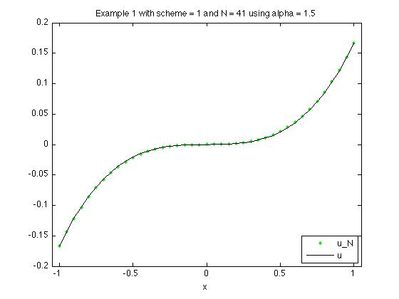
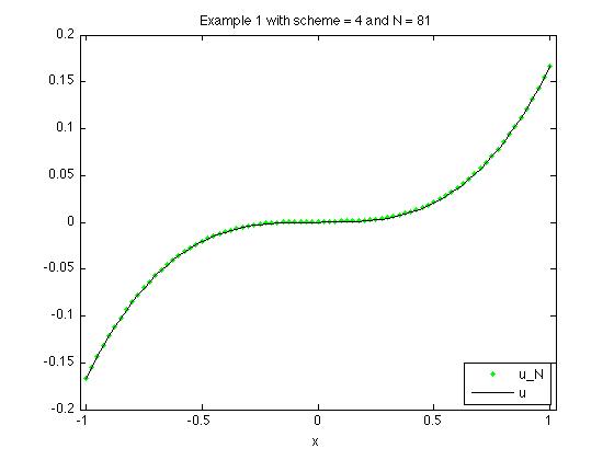
Fig. 1: Computed solutions of Example 1

The schemes $\widehat{F}_{2}$ and $\widehat{F}_{3}$ exhibit similar behavior as $\widehat{F}_{1}$, and $\widehat{F}_{5}$ exhibits similar behavior as $\widehat{F}_{4}$. Thus, the Lax-Friedrichs-like schemes do exhibit a quadratic order of convergence as expected. On the other hand, the Godunov-like schemes converge inconsistently. This inconsistency is mostly due to fsolve failing to find a root.

If we fix our initial guess as the approximation computed by $\widehat{F}_{1}$ with $\alpha=1.5$ and $h=0.1$, we get the results of Table 2.

	$\widehat{F}_{1}$ , $\alpha=1.5$		$\widehat{F}_{4}$
$h$	$L^{\infty}$ error	order	$L^{\infty}$ error	order
1.0000e-01	2.71e-02		8.24e-08
5.0000e-02	5.10e-03	2.41	1.58e-06	-4.26
2.5000e-02	1.03e-03	2.31	1.60e-05	-3.34
1.2500e-02	2.33e-04	2.14	9.06e-05	-2.51
6.2500e-03	5.58e-05	2.06	1.42e-02	-7.29

Table 2: Rates of convergence of Example 1.

Thus, Godunov-like schemes converge with high levels of accuracy when the nonlinear solver has a sufficiently good initial guess. Since the Godunov-like schemes are very sensitive towards the initial guess for fsolve, it is hard to characterize a rate of convergence. We also observe in Table 1 that the error for $h=0.1,0.05,0.025,0.00625$ is consistent with the error of the initial guess for the Godunov-like schemes. In contrast, the Lax-Friedrichs-like schemes converge for a much wider range of initial guesses.

The next example concerns the 1-D Monge-Ampere equation.

Example 2: Consider the problem

$$-u_{xx}^{2}+1 =0,\qquad 0<x<1,$$

$$u(0)=0,\quad u(1) =1/2.$$

This problem has exactly two solutions

$$u^{+}(x)=\frac{1}{2}x^{2},\qquad u^{-}(x)=-\frac{1}{2}x^{2}+x,$$

where $u^{+}$ is convex and $u^{-}$ is concave. However, $u^{+}$ is the unique viscosity solution that preserves the ellipticity of the operator.

Using $U^{(0)}$ as the linear interpolant of the boundary data, the computed results with both types of schemes are given in Table 3.

	$\widehat{F}_{1}$ , $\alpha=1$		$\widehat{F}_{1}$ , $\alpha=-1$		$\widehat{F}_{4}$
$h$	$L^{\infty}$ error	order	$L^{\infty}$ error	order	$L^{\infty}$ error	order
1.000e-01	2.54e-03		2.54e-03		1.17e-01
5.000e-02	6.36e-04	2.00	6.36e-04	2.00	1.21e-01	-0.05
2.500e-02	1.59e-04	2.00	1.59e-04	2.00	1.24e-01	-0.04

Table 3: Rates of convergence of Example 2.

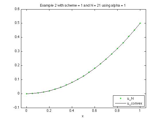
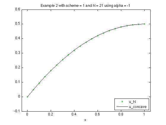
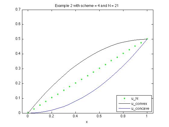
Fig. 2: Computed solutions of Example 2 with different parameter $\alpha$.

We note that the Lax-Friedrichs-like schemes converge to the unique ellipticity preserving solution (i.e., convex solution) for $\alpha>0$ sufficiently large. However, if $\alpha<0$ with $\left|\alpha\right|$ sufficiently large, the Lax-Friedrichs-like schemes converge to $u^{-}$. The convergence to $u^{-}$ for $\alpha<0$ is expected since $u^{-}$ is the unique solution that preserves the ellipticity of the PDE $u_{xx}^{2}-1=0$. Forming the corresponding Lax-Friedrichs-like scheme and multiplying by $-1$ is equivalent to letting $\alpha<0$ in the above formulation.

We also test the benefit of using a Lax-Friedrichs-like scheme as opposed to the standard $3$-point finite difference method. We approximate $u$ using $\widehat{F}_{2}$ for varying values of $\alpha$, using the linear interpolant of the boundary data as our initial guess. The computed results are given in Table 4.

	$\widehat{F}_{2}$ , $\alpha=6$		$\widehat{F}_{2}$ , $\alpha=0.05$		$\widehat{F}_{2}$ , $\alpha=0$
$h$	$L^{\infty}$ error	order	$L^{\infty}$ error	order	$L^{\infty}$ error	order
1.000e-01	3.07e-02		1.18e-01		9.00e-02
5.000e-02	8.51e-03	1.85	3.31e-02	1.83	1.15e-01	-0.35
2.500e-02	2.14e-03	1.99	3.03e-02	0.13	1.15e-01	-0.00

Table 4: Performance of a Lax-Friedrichs-like scheme with various $\alpha$

hb

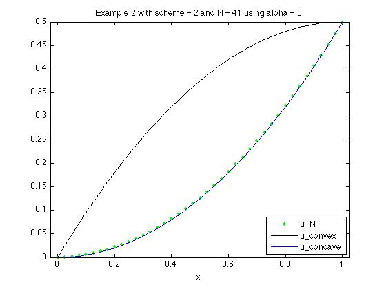
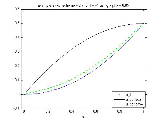
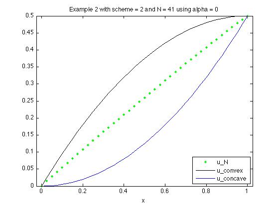
Fig. 3: Computed solutions by a Lax-Friedrichs-like scheme with various $\alpha$

We remark that letting $\alpha=0$ corresponds to the standard $3$-point finite difference method, which does not converge in the above example. Instead, it behaves similarly to the Godunov-like schemes in that the nonlinear solver cannot determine a good direction to move from the initial guess. Thus, the Lax-Friedrichs-like schemes have a mechanism for giving the nonlinear solver a good direction towards finding a root. When $\alpha$ is sufficiently large, the schemes converge. When $\alpha$ is not sufficiently large, while the schemes may not converge, they have a tendency to move towards the correct solution. Furthermore, we can see that the Lax-Friedrichs-like schemes converge quadratically for $\alpha$ bigger than the theoretical lower bound with only a small cost in the level of accuracy. Thus, when dealing with a problem that has an unknown optimal bound for $\alpha$, large $\alpha$ values can be used. A shooting method for decreasing $\alpha$ allows the scheme to gain accuracy while maintaining the benefits of the Lax-Friedrichs-like schemes.

If we first use $\widehat{F}_{1}$ with $\alpha=1$ to approximate $u$ on a coarse mesh with $h=0.1$, and then we interpolate the result to get an initial guess for the two proposed schemes and the $3$-point finite difference method, we get the results of Table 5. Thus, we see that the Godunov-like schemes and the standard finite difference formulation now converge to $u^{+}$ with high levels of accuracy given a sufficiently good initial guess. In fact, they both converge to the same limit.

	$\widehat{F}_{1}$ , $\alpha=1$		$\widehat{F}_{4}$		$\widehat{F}_{2}$ , $\alpha=0$
$h$	$L^{\infty}$ error	order	$L^{\infty}$ error	order	$L^{\infty}$ error	order
1.000e-01	2.54e-03		9.96e-15		9.96e-15
5.000e-02	6.36e-04	2.00	4.54e-13	-5.51	4.54e-13	-5.51
2.500e-02	1.59e-04	2.00	1.46e-10	-8.33	1.46e-10	-8.33
1.250e-02	3.97e-05	2.00	9.85e-10	-2.75	9.85e-10	-2.75

Table 5: Performance of the standard $3$-point scheme

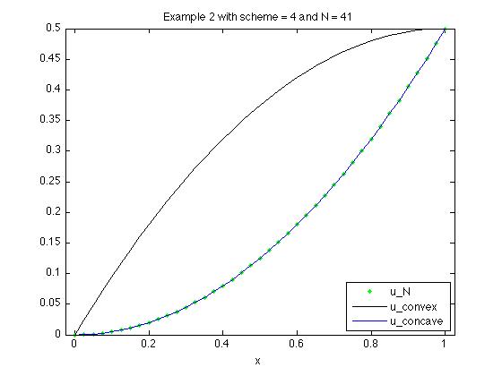
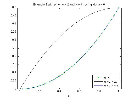
Fig. 4: Computed solutions by a Godunov-like scheme and the standard $3$-point scheme

To the contrary, if we use $\widehat{F}_{1}$ with $\alpha=-1$ to approximate $u$ on a coarse mesh with $h=0.1$ and then interpolate the result as an initial guess, we obtain the results of Table 6. Clearly, none of the schemes converge to $u^{+}$. Moreover, the Lax-Friedrichs-like schemes and the Godunov-like schemes do not converge to $u^{-}$ even if $U^{0}$ is close to $u^{-}$. Instead, fsolve finds no solution when using the two proposed schemes. Thus, the Lax-Friedrichs-like schemes and the Godunov-like schemes appear to only consider $u^{+}$ to be the solution of the PDE. Since $u^{+}$ is the unique viscosity solution of the PDE, lack of convergence to $u^{-}$ for the Lax-Friedrichs-like schemes for $\alpha>0$ sufficiently large and for the Godunov-like schemes is consistent with theory.

In contrast, the standard $3$-point finite difference method does converge to $u^{-}$. When given a sufficiently good guess, the $3$-point finite difference method will converge to any one of the two solutions. Furthermore, the discretization can create artificial solutions that will attract the standard $3$-point finite difference method. On the other hand, the monotonicity of our proposed schemes prevent the discretizations from having multiple solutions.

	$\widehat{F}_{1}$ , $\alpha=-1$		$\widehat{F}_{4}$		$\widehat{F}_{2}$ , $\alpha=0$
$h$	$L^{\infty}$ error	order	$L^{\infty}$ error	order	$L^{\infty}$ error	order
1.000e-01	2.68e-02		2.56e-03		2.24e-14
5.000e-02	5.61e-03	2.25	2.54e-03	0.01	8.82e-13	-5.30
2.500e-02	1.26e-02	-1.16	2.54e-03	0.00	8.83e-12	-3.32
1.250e-02	1.41e-02	-0.17	2.54e-03	-0.00	1.63e-09	-7.53

Table 6: Performance of a Lax-Friedrichs-like scheme with $\alpha=-1$.

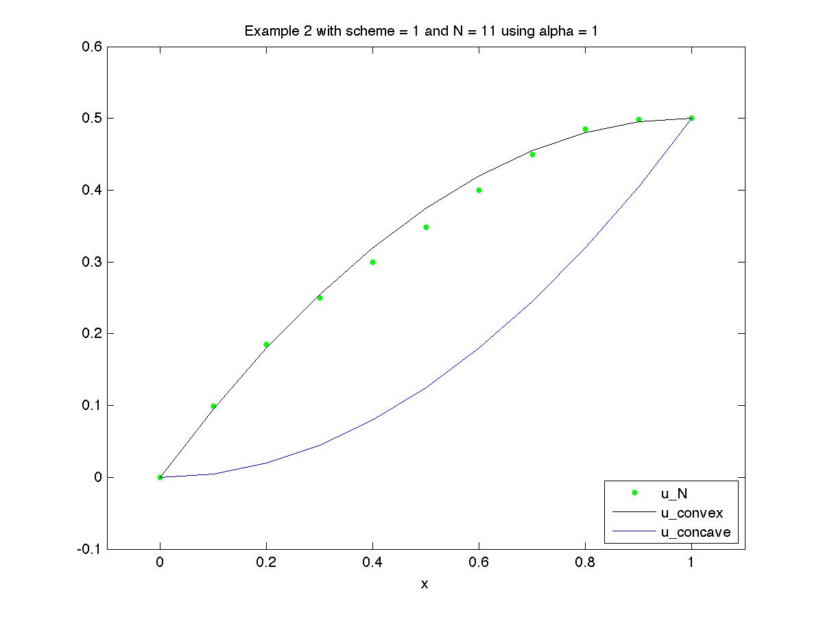
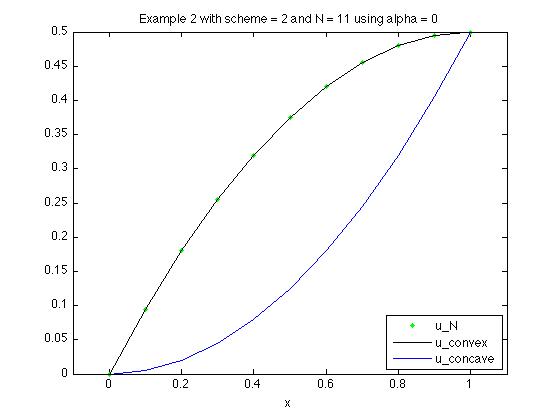
Fig. 5: Computed solutions of a Lax-Friedrichs-like scheme with $\alpha=-1$.

The next two examples deals with Bellman type equations.

Example 3: Consider the problem

$$\min_{\theta(x)\in\left\{1,2\right\}}\bigl{\{}-A_{\theta}u_{xx}-S\left(x\right)\bigr{\}} =0,\qquad-1<x<1,$$

$$u(-1)=-1,\quad u(1) =1.$$

for

$$A_{1}=1,\quad A_{2}=2,\quad S(x)=\begin{cases}12x^{2},&\text{if }x<0,\\ -24x^{2},&\text{if }x\geq 0.\end{cases}$$

This problem has the exact solution $u(x)=x\left|x\right|^{3}$. We also note that this problem has a finite dimensional control parameter set.

Using the linear interpolant as the initial guess, we obtain the results of Table 7. We observe that the Godunov-like scheme converges and both schemes exhibit quadratic convergence for this example.

	$\widehat{F}_{1}$ , $\alpha=1$		$\widehat{F}_{4}$
$h$	$L^{\infty}$ error	order	$L^{\infty}$ error	order
1.000e-01	1.29e-01		9.60e-03
5.000e-02	4.67e-02	1.46	2.50e-03	1.94
2.500e-02	1.46e-02	1.68	6.25e-04	2.00
1.250e-02	4.18e-03	1.80	4.70e-01	-9.55
6.250e-03	1.13e-03	1.89	4.72e-01	-0.01
3.125e-03	2.95e-04	1.93	4.72e-01	-0.00

Table 7: Rates of convergence of Example 3.

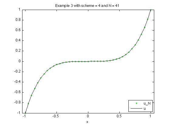
Fig. 6: Computed solutions of Example 3.

Now we consider a Bellman problem with infinite dimensional control parameter set.

Example 4: Let $\theta:\mathbb{R}\to\mathbb{R}$ such that $\theta\in L^{\infty}([2,4])$, and consider the problem

$$\inf_{-1\leq\theta(x)\leq 1}\bigl{\{}-\theta\,u_{xx}+\theta^{2}\,u+x^{-2}\bigr{\}} =0,\qquad 2<x<4,$$

$$u(2)=4,\quad u(4) =16.$$

This problem has the exact solution $u(x)=x^{2}$ with the corresponding control $\theta(x)=x^{-2}$.

Let the initial guess be given by the linear interpolant of the boundary data. Then, we obtain the results of Table 8.

	$\widehat{F}_{1}$ , $\alpha=0.5$		$\widehat{F}_{4}$
$h$	$L^{\infty}$ error	order	$L^{\infty}$ error	order
1.000e-01	3.07e-01		5.59e-01
5.000e-02	9.88e-02	1.64	4.96e-01	0.17
2.500e-02	3.09e-02	1.68	5.10e+00	-3.36

Table 8: Rates of convergence of Example 4.

Both schemes have a hard time finding a root for $h$ small, although the Lax-Friedrichs-like schemes do converge towards $u$ for larger values of $h$.

Now we choose the initial guess

$$U^{(0)}=\frac{3}{14}x^{3}+\frac{16}{7},$$

a simple cubic function that satisfies the boundary conditions. Then, $\|U^{(0)}$ $-u\|_{L^{\infty}([2,4])}\approx 0.94$, and we get the results of Table 9.

	$\widehat{F}_{1}$ , $\alpha=0.5$		$\widehat{F}_{4}$
$h$	$L^{\infty}$ error	order	$L^{\infty}$ error	order
1.000e-01	3.07e-01		6.74e-10
5.000e-02	9.88e-02	1.64	7.04e-08	-6.71
2.500e-02	3.09e-02	1.68	3.41e-09	4.37
1.250e-02	9.02e-03	1.78	8.09e-08	-4.57
6.250e-03	2.47e-03	1.87	9.44e-01	-23.48

Table 9: Rates of convergence of Example 4.

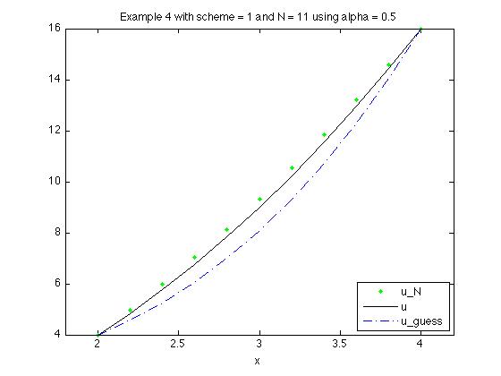
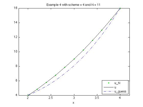
Fig. 7: Computed solutions of Example 4.

Thus, the Lax-Friedrichs-like schemes again converge with a rate of almost $2$. Also, the Godunov-like schemes converge with high levels of accuracy for $h\geq 0.0125$, but for smaller $h$, fsolve fails to find a root .

We remark that this problem can also be approximated by using a splitting algorithm. The operator can be split into an optimization problem for $\theta$ and a linear PDE problem for $u$, and then a natural scheme is to successively approximate $\theta$ and $u$ starting with an initial guess for $\theta$. For the above approximations, the nonlinearity due to the infimum was preserved inside the definition of the operator.

The final example considers a problem whose solution is not classical.

Example 5: Consider the problem

$$-u_{xx}^{3}+8\text{ sign}(x) =0,\qquad-1<x<1,$$

$$u(-1)=-1,\quad u(1) =1,$$

with the exact solution $u(x)=x|x|\in C^{1}([-1,1])$.

Using the linear interpolant of the boundary data as the initial guess, we obtain the results of Table 10.

	$\widehat{F}_{1}$ , $\alpha=1.5$		$\widehat{F}_{4}$
$h$	$L^{\infty}$ error	order	$L^{\infty}$ error	order
1.000e-01	1.59e-02		2.40e-01
5.000e-02	3.76e-03	2.08	2.50e-01	-0.06
2.500e-02	9.40e-04	2.00	2.50e-01	0.00
1.250e-02	2.35e-04	2.00	6.69e-06	15.19
6.250e-03	5.88e-05	2.00	2.05e-01	-14.90

Table 10: Rates of convergence of Example 5.

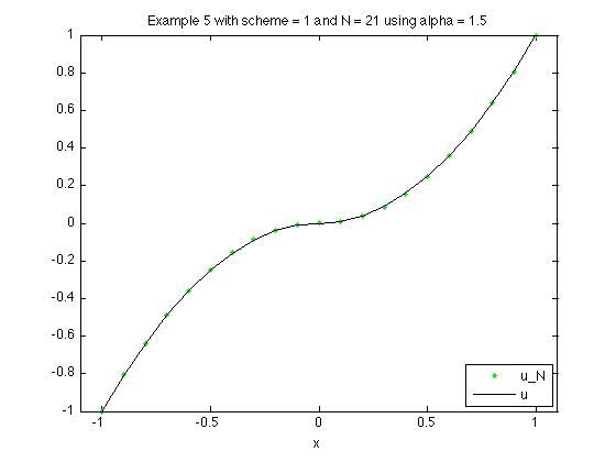
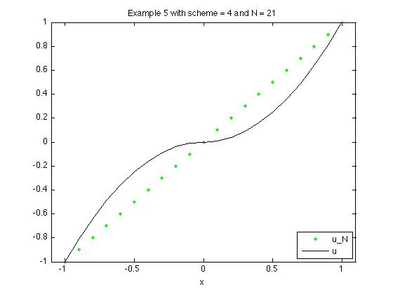
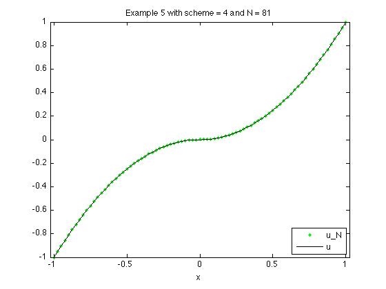
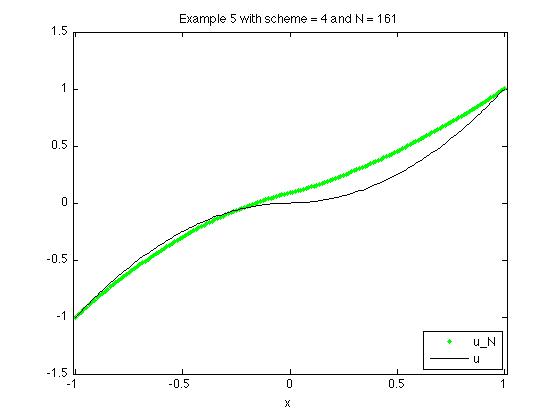
Fig. 8: Computed solutions of Example 4.

We clearly see the quadratic rate of convergence for the Lax-Friedrichs-like schemes. The Godunov-like schemes only converge for $h=0.0125$. For larger $h$, the scheme returns the initial guess after failing to find a root. For the test with smaller $h$, the scheme returns a slightly improved approximation after reaching the maximum number of iterations.

If we fix our initial guess as the approximation formed by $\widehat{F}_{1}$ with $\alpha=1.5$ and $h=0.1$, we then get the results of Table 11.

	$\widehat{F}_{1}$ , $\alpha=1.5$		$\widehat{F}_{4}$
$h$	$L^{\infty}$ error	order	$L^{\infty}$ error	order
1.000e-01	1.59e-02		1.84e-08
5.000e-02	3.76e-03	2.08	4.05e-06	-7.78
2.500e-02	9.40e-04	2.00	8.85e-06	-1.13
1.250e-02	2.35e-04	2.00	6.50e-06	0.45
6.250e-03	5.88e-05	2.00	7.78e-06	-0.26

Table 11: Rates of convergence of Example 5.

As observed in the previous examples, we see that the Godunov-like schemes converge quickly with high levels of accuracy, thus making it difficult to characterize a general rate of convergence.

6 Conclusion

We have presented a new framework for constructing and analyzing consistent, g-monotone, and stable finite difference methods. The newly proposed consistency and g-monotonicity criterion are not only simple to understand, but they are also easy to verify in practice. The key concept of the framework is the “numerical operator”, which plays the same role as the “numerical Hamiltonian” does in the successful monotone finite difference framework for first order fully nonlinear Hamilton-Jacobi equations. To construct practically useful finite difference methods which can be easily implemented on computers, we have also presented a guideline for designing finite difference methods which fulfill the structure criterion of the proposed finite difference framework. The key concept in this regard is the “numerical moment”, which plays the same role as the “numerical viscosity” does in the successful finite difference framework for first order fully nonlinear Hamilton-Jacobi equations. Moreover, we gave some numerical evidences and argued that “numerical moments” provide an indispensable mechanism and ability for a finite difference scheme to be able to converge to the viscosity solution of the underlying second order fully nonlinear PDE problem. To a certain degree, the work of this paper bridges the gap between the state-of-the-art of finite difference methods for second order fully nonlinear PDEs and that for first order fully nonlinear Hamilton-Jacobi equations. Although the results of this paper are confined to the one spatial dimension case, they are also expected to hold in high spatial dimensions; that result will be presented in a forthcoming companion paper [15].

References

- [1] M. Bardi, I. Capuzzo-Dolcetta, Optimal control and viscosity solutions of Hamilton-Jacobi-Bellman equations, Systems & Control: Foundations & Applications, Birkhäuser Boston Inc., Boston, MA, 1997, with appendices by Maurizio Falcone and Pierpaolo Soravia.
- [2] G. Barles, P. E. Souganidis, Convergence of approximation schemes for fully nonlinear second order equations, Asymptotic Anal. 4 (3) (1991) 271–283.
- [3] G. Barles, E. R. Jakobsen, Error bounds for monotone approximation schemes for parabolic Hamilton-Jacobi-Bellman equations, Math. Comp. 76(2007) 1861-1893.
- [4] L. A. Caffarelli, X. Cabré, Fully nonlinear elliptic equations, Vol. 43 of American Mathematical Society Colloquium Publications, American Mathematical Society, Providence, RI, 1995.
- [5] L. A. Caffarelli, P. A. Souganidis, A rate of convergence for monotone finite difference approximations to fully nonlinear, uniformly elliptic PDEs, Comm. Pure Appl. Math. 61 (2008) 1–17.
- [6] M. G. Crandall, P.-L. Lions, Viscosity solutions of Hamilton-Jacobi equations, Trans. Amer. Math. Soc. 277 (1) (1983) 1–42.
- [7] M. G. Crandall, P. L. Lions, Two approximations of solutions of Hamilton-Jacobi equations, Math. Comp. 43 (1984) 1–19.
- [8] M. G. Crandall, L. Tartar, Some relations between nonexpansive and order preserving mappings, Proc. Amer. Math. Soc. 79 (1979) 74–80.
- [9] E. J. Dean, R. Glowinski, Numerical solution of the two-dimensional elliptic Monge-Ampère equation with Dirichlet boundary conditions: an augmented Lagrangian approach, C. R. Math. Acad. Sci. Paris 336 (9) (2003) 779–784.
- [10] E. J. Dean, R. Glowinski, Numerical methods for fully nonlinear elliptic equations of the Monge-Ampère type, Comput. Methods Appl. Mech. Engrg. 195 (13-16) (2006) 1344–1386.
- [11] D. Gilbarg, N. S. Trudinger, Elliptic partial differential equations of second order, Classics in Mathematics, Springer-Verlag, Berlin, 2001, reprint of the 1998 edition.
- [12] X. Feng, M. Neilan, Mixed finite element methods for the fully nonlinear Monge-Ampére equation based on the vanishing moment method, SIAM J. Numer. Anal. 47 (2009) 1226–1250.
- [13] X. Feng, R. Glowinski, M. Neilan, Recent developments in numerical methods for second order fully nonlinear PDEs, to appear in SIAM Review.
- [14] X. Feng, M. Neilan, The vanishing moment method for fully nonlinear second order partial differential equations: formulation, theory, and numerical analysis, arxiv.org/abs/1109.1183v2.
- [15] X. Feng, C. Y. Kao, T. Lewis, Monotone finite difference methods for the fully nonlinear Monge-Ampère and Bellman equations in high dimensions, in preparation.
- [16] N. Krylov, Rate of convergence of difference approximations for uniformly nondegenerate elliptic Bellman’s equations, arXiv:1203.2905 [math.AP].
- [17] H. J. Kuo, N. S. Trudinger, Discrete methods for fully nonlinear elliptic equations, SIAM J. Numer. Anal. 29 (1) (1992) 123–135.
- [18] G. M. Lieberman, Second order parabolic differential equations, World Scientific Publishing Co. Inc., River Edge, NJ, 1996.
- [19] A. M. Oberman, Wide stencil finite difference schemes for the elliptic Monge-Ampère equation and functions of the eigenvalues of the Hessian, Discrete Contin. Dyn. Syst. Ser. B 10 (1) (2008) 221–238.
- [20] C.-W. Shu, High order numerical methods for time dependent Hamilton-Jacobi equations, in: Mathematics and computation in imaging science and information processing, Vol. 11 of Lect. Notes Ser. Inst. Math. Sci. Natl. Univ. Singap., World Sci. Publ., Hackensack, NJ, 2007, pp. 47–91.
- [21] J. Yan, S. Osher, Direct discontinuous local Galerkin methods for Hamilton-Jacobi equations, J. Comp. Phys. 230 (2011) 232–244.