Closed and Open System Dynamics in a Fermionic Chain with a Microscopically Specified Bath: Relaxation and Thermalization

Abstract

We study thermalization in a one-dimensional quantum system consisting of a noninteracting fermionic chain with each site of the chain coupled to an additional bath site. Using a density matrix renormalization group algorithm we investigate the time evolution of observables in the chain after a quantum quench. For low densities we show that the intermediate time dynamics can be quantitatively described by a system of coupled equations of motion. For higher densities our numerical results show a prethermalization for local observables at intermediate times and a full thermalization to the grand canonical ensemble at long times. For the case of a weak bath-chain coupling we find, in particular, a Fermi momentum distribution in the chain in equilibrium in spite of the seemingly oversimplified bath in our model.

Introduction.

The time evolution of classical and quantum systems is deterministic. If a system in the thermodynamic limit reaches thermal equilibrium at long times, we expect, however, that its physical properties will be determined by only a few parameters such as the temperature, chemical potential, and pressure. This thermalization process is often studied in two different settings: (a) The system is in contact with a thermal bath, i.e., a large reservoir of thermal energy. The key assumptions commonly used in this setting are a weak coupling between the bath and system and Markovian dynamics, i.e., a very short correlation time in the bath. In this case the microscopic details of the bath become unimportant Breuer and Petruccione (2002); Weiss (2008); Carmichael (1998); for a simple example of classical thermalization, see Ref. gebhardmuenster (2011). (b) The system is closed, with particles being able to exchange energy and momentum among each other, so that the closed system can explore phase space, constrained only by the conservation laws such as total energy and particle number. An important difference between the two scenarios is that in the first case temperature, chemical potential, and pressure are parameters determined externally by the bath. In the latter case, on the other hand, these parameters are Lagrange multipliers fixing the values of the conserved quantities Landau and Lifshitz (1980); Rigol et al. (2008).

In this letter we want to study these two settings simultaneously using a model which can be either viewed as a closed quantum system or as a chain coupled to a simple bath. Thermalization, in both cases, requires: (I) Observables become time independent and all currents vanish (equilibration); (II) Time averages can be replaced by statistical averages over ensembles with a restricted number of intensive parameters , and are independent of initial conditions (ergodicity) von Neumann (1929). The rather old but fundamental problem of nonequilibrium dynamics and thermalization in closed quantum systems has been put again into focus by experiments on cold quantum gases which are very well isolated from their surroundings Trotzky et al. (2012); Kinoshita et al. (2006); Hofferberth et al. (2007); Strohmaier et al. (2010), as well as by the development of new numerical techniques to study dynamics in many-body systems Daley et al. (2004); White and Feiguin (2004); Sirker and Klümper (2005); Vidal (2003, 2004); Enss and Sirker (2012); Anders and Schiller (2005); Kehrein (2005). This has led to numerous simulations of nonequilibrium dynamics in closed quantum models where the question of whether or not thermalization occurs has not always been easy to answer due to the finite numerical simulation time Rigol et al. (2006); Kollath et al. (2007); Manmana et al. (2007); Biroli et al. (2010).

Closed quantum systems.

The time evolution of an initial state $|\Psi_{0}\rangle\equiv|\Psi(t=0)\rangle$ is unitary and given by the Schrödinger equation. Therefore $|\Psi(t)\rangle$ remains a pure state for all times $t$. Since ensemble averages describe mixed states such a description cannot apply to a finite closed quantum system as a whole. Only a subsystem can be in or close to a thermal state with the rest of the system acting as an effective bath. Furthermore, contrary to a classical system, every quantum system has exponentially many conserved quantities, e.g. the projection operators $P_{n}=|E_{n}\rangle\langle E_{n}|$ onto the eigenstates of a system with a discrete spectrum, $|E_{n}\rangle$ Rigol et al. (2008). However, it is usually assumed that only the local conserved quantities are of relevance for thermalization. A local conserved quantity can be represented for a lattice system as $Q_{m}=\sum_{j}q^{m}_{j}$ where $q^{m}_{j}$ is a density operator acting on lattice sites $j,j+1,\cdots,j+m$ with $m$ finite. Here we want to concentrate on the case of generic one-dimensional quantum systems with a small number of local conservation laws, i.e. the total energy and particle number. Thermalization in closed integrable models, where the number of local conservation laws increases linearly with the system size Essler et al. (2005); Sirker (2012), has been investigated with the help of numerical simulations in recent times as well Rigol et al. (2007); Rigol (2009a, b); Santos and Rigol (2010).

We consider the nonequilibrium dynamics ensuing after preparing the system in a pure state $|\Psi_{0}\rangle$ which is not an eigenstate of the Hamiltonian. Using a Lehmann representation we can write $|\Psi_{0}\rangle=\sum_{n}c_{n}|E_{n}\rangle$ where $|E_{n}\rangle$ are the eigenstates of the Hamiltonian $H$ the system evolves under. Furthermore, we restrict ourselves to typical states with a macroscopic number $c_{n}\neq 0$ . We can now easily calculate the long-time mean

$$\bar{O} = \lim_{\tau\to\infty}\sum_{n,m}\frac{1}{\tau}\int_{0}^{\tau}\textrm{d}t\,\text{e}^{\textrm{i}(E_{m}-E_{n})t}c_{n}^{*}c_{m}\langle E_{m}|O|E_{n}\rangle$$ (1)

$$= \sum_{n}|c_{n}|^{2}O_{nn}$$

of an observable $O$, where we have set $\hbar=1$. The second line of Eq. (1) is often called the diagonal ensemble. Here we have assumed that the system is generic, i.e., that degeneracies play no role. If the observable becomes stationary at long times its value $O_{\infty}=\lim_{t\to\infty}\langle\psi(t)|O|\psi(t)\rangle$ has to be equal to the long-time mean, $O_{\infty}\equiv\bar{O}$. Note that this is only possible in the thermodynamic limit. Otherwise observables show revivals on time scales of the order of the system size. Taking the thermodynamic limit is thus essential; a finite system can never thermalize.

If a subsystem of an infinite system containing the observable $O$ equilibrates and the value $O_{\infty}$ does not depend on details of the initial state, then the remaining open question is which ensemble describes the equilibrated system. If we have two statistically independent subsystems $A$ and $B$, the density matrix $\rho$ of the whole system is given by $\rho=\rho_{A}\otimes\rho_{B}$, and thus $\ln\rho=\ln\rho_{A}\oplus\ln\rho_{B}$. Second, the density matrix itself should become time independent once the system has equilibrated and the von Neumann equation implies $\dot{\rho}=-\textrm{i}[H,\rho]=0$. Thus the general density matrix under consideration has to be of the form $\rho=\exp(-\sum_{n}\lambda_{n}\mathcal{Q}_{n})/Z$ where $\mathcal{Q}_{n}$ are the conserved quantities of the system Landau and Lifshitz (1980). The partition function $Z$ is a normalization factor such that $\operatorname{Tr}\rho=1$. We stress again that the intensive parameters $\lambda_{n}$ are not given externally but rather are Lagrange multipliers determined by the set of equations

$$\langle\Psi_{0}|\mathcal{Q}_{n}|\Psi_{0}\rangle=\operatorname{Tr}\left\{\mathcal{Q}_{n}\rho\right\}.$$ (2)

If we include all projection operators into our density matrix, $\mathcal{Q}_{n}=P_{n}$, it follows immediately from Eq. (2) that $\langle O\rangle_{\rho}\equiv\operatorname{Tr}\{\rho O\}$ is identical to the diagonal ensemble as given in Eq. (1) Rigol et al. (2008). Having to use infinitely many Lagrange multipliers is expected because $|\Psi(t)\rangle$ is always a pure state and the system as a whole therefore does not thermalize, because it does not fulfill condition (II).

In this Letter we focus on the generic situation where we split our system $S=A\cup B$ into a bath $B$ and a subsystem $A$ and consider observables acting only on subsystem $A$. We concentrate on the following questions: How does a subsystem $A$ without intrinsic relaxation processes equilibrate when coupled to a strongly correlated but simple and possibly non-Markovian bath $B$? Which statistical ensemble gives the expectation values of observables in $A$ in the equilibrated state?

Model Hamiltonian.

To investigate some aspects of the questions raised above we consider a simple model system with Hamiltonian Gebhard et al. (2012)

$$H = -J\sum_{j=1}^{L-1}\left\{c_{j}^{\dagger}c_{j+1}+h.c.\right\}+\gamma\sum_{j=1}^{L}\left\{s^{\dagger}_{j}c_{j}+\textrm{H.c.}\right\}$$ (3)

$$+V_{s}\sum_{j=1}^{L-1}\left(s_{j}^{\dagger}s_{j}-1/2\right)\left(s^{\dagger}_{j+1}s_{j+1}-1/2\right)\;.$$

The first term describes a chain of free spinless fermions with hopping amplitude $J$ and is the subsystem $A$ we study the thermalization of. The ‘bath’ $B$ consists of extra sites, coupled to the chain sites via a hybridization $\gamma$ (second term), and we also include a nearest-neighbor interaction $V_{s}$ between the bath sites (third term).

As initial states for the time-evolution with the Hamiltonian (3) we will consider, on the one hand, the ground state $|\Psi_{0}^{\textrm{I}}(J_{0},\gamma_{0})\rangle\equiv|\Psi(J_{0},\gamma_{0},V_{s}=0)\rangle_{0}$ of the noninteracting model with hopping parameters $J_{0}$ and $\gamma_{0}$ as well as the ground state $|\Psi_{0}^{\textrm{II}}(J_{0},J^{\prime}_{0},\gamma_{0})\rangle\equiv|\Psi(J_{0},J^{\prime}_{0},\gamma_{0},V_{s}=0)\rangle_{0}$ of Eq. (3) with an additional hopping $J^{\prime}_{0}$ between the bath sites. In order to study the time evolution under the interacting Hamiltonian we use a time-dependent density-matrix renormalization group (DMRG) algorithm Feiguin and White (2005), a method which has already been applied to study other one-dimensional models Kollath et al. (2007); Manmana et al. (2007); Heidrich-Meisner et al. (2008). We choose open boundary conditions with a chain length of $L=51$. The number of states kept in the truncated adaptive Hilbert space varies between $\chi=400$ and $\chi=800$. For a global quench as considered here it is well known that the entanglement entropy between two subsystems usually increases linearly with time. Since the maximal entanglement which can be represented in a truncated Hilbert space is limited by $\ln\chi$, there is a maximum time $t_{\rm max}$ up to which we can reliably simulate the time evolution. For the cases considered here this time scale is given by $Jt_{\rm max}\approx 15-25$.

Results.

First, we will concentrate on the relaxation dynamics at low particle densities. As an example, we show in Fig. 1 results for a quantum quench with $N=11$ particles. Shown are results for the one–point correlation functions

$$C_{j}(t)\equiv\langle\hat{C}_{j}\rangle_{t}=\langle\Psi(t)|c_{(L+1)/2}^{\dagger}c_{(L+1)/2+j}|\Psi(t)\rangle\;.$$ (4)

In all correlation functions oscillations with a characteristic frequency are visible. These oscillations can be understood from an equation of motion approach. We define the three time-dependent expectation values $f_{q}(t)=\langle\Psi(t)|c^{\dagger}_{q}c_{q}|\Psi(t)\rangle$, $g_{q}(t)=\langle\Psi(t)|s^{\dagger}_{q}s_{q}|\Psi(t)\rangle$, and $\rho_{q}(t)=\langle\Psi(t)|c^{\dagger}_{q}s_{q}|\Psi(t)\rangle$ where $c_{q}=\sqrt{2/(L+1)}\sum_{j}\sin(qj)c_{j}$ with allowed momenta $q=n\pi/(L+1)$, and $n=1,\ldots,L$. Then, using Heisenberg’s equation of motion, a Hartree-Fock decoupling of the quartic terms, and the additional assumption of an instantaneous dephasing Sup , we find the following system of coupled equations

$$\dot{f}_{q}(t) = -\dot{g}_{q}(t)=2\gamma R_{q}(t)\;,\quad\dot{r}_{q}(t)=B_{q}(t)R_{q}(t)\;,$$

$$\dot{R}_{q}(t) = -\gamma[f_{q}(t)-g_{q}(t)]-B_{q}(t)r_{q}(t)\;,$$ (5)

with $\varepsilon_{q}=-2\cos q$, $r_{q}(t)=\operatorname{Re}\rho_{q}(t)$, $R_{q}(t)=\operatorname{Im}\rho_{q}(t)$, and $B_{q}(t)=-V_{s}-\varepsilon_{q}+2V_{s}/(L+1)\bigl{[}\cos^{2}(q)g_{\pi-q}(t)-\sin^{2}(q)g_{q}(t)+\sum_{k}\bigl{(}1-\cos k\cos q\bigr{)}g_{k}(t)\bigr{]}\approx-V_{s}-\varepsilon_{q}\equiv\mathcal{B}_{q}$.

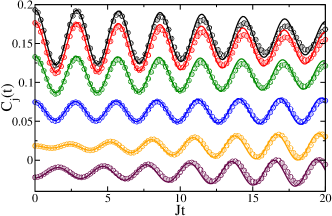
Figure 1: (Color online) $C_{j}(t)$ from Eq. (4) for $j=0,\ldots,5$ (top to bottom) for a quench with initial state $|\Psi_{0}^{\textrm{I}}(1,1)\rangle$, and Hamiltonian $H$ with $J=1$, $\gamma=1$, and $V_{s}=1$ at low densities. DMRG results (symbols) are compared to the solution of Eq. (Results.) (lines).

We solve the set of Eqs. (Results.) numerically, and the results up to intermediate times are in excellent agreement with the DMRG data, see Fig. 1. Using further approximations, we analytically find that the oscillation frequency is given by $\Omega^{2}_{q}=\mathcal{B}_{q}^{2}+(2\gamma)^{2}$ with $\Omega^{2}_{q\to 0}\approx 1+(2\gamma)^{2}$ and depends only weakly on $q$ Sup . This means that the dephasing process is very slow. For longer times and short distances we see that the amplitude of the oscillations in the DMRG data is decaying faster than predicted by our equations of motion approach. Here it is important to realize that due to the Hartree-Fock decoupling the equations of motion effectively describe the time evolution under a free particle Hamiltonian. This approach therefore takes only the slow dephasing process discussed above into account. The additional decay seen in the DMRG data is due to slow relaxation processes involving energy-momentum transfer between interacting particles which are not captured in our equations of motion approach.

A much faster relaxation occurs if we increase the particle density with a maximum in the relaxation rate at half filing. The DMRG data for a quench in the half-filled case in Fig. 2 show indeed that the system almost completely equilibrates within the simulation time $t_{\textrm{max}}$.

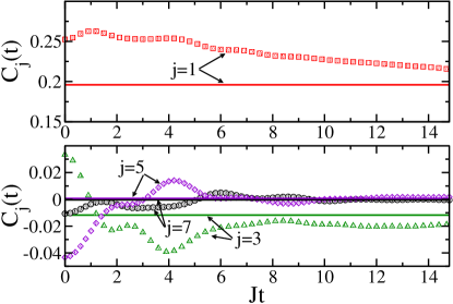
Figure 2: (Color online) DMRG data (symbols) for $C_{j}(t)$ at half filing for a quench with initial state $|\Psi_{0}^{\textrm{II}}(1,0.6,1)\rangle$, and Hamiltonian $H$ with $J=1$, $\gamma=1$, and $V_{s}=1$. The lines are the thermal expectation values $\langle C_{j}\rangle_{T}$.

Due to the particle–hole symmetry of the Hamiltonian and the initial state we have $C_{0}(t)\equiv 1/2$ and $C_{2j}(t)\equiv 0$. For odd distances we now see, instead of long-time oscillations, an exponential damping which allows us to extrapolate the correlation functions and to read off the value for $C_{j}(t\to\infty)$ Sup . Due to the lightcone-like spreading of the correlations Lieb and Robinson (1972); Enss and Sirker (2012), the short-range correlation functions in the middle of the chain are, for the time range shown in Fig. 2, not affected by the boundaries and are almost indistinguishable from those for an infinite system. By extrapolating our numerical data we thus approximately obtain $C_{j}(t\to\infty)$ for a system in the thermodynamic limit.

The corresponding distribution function $f_{q}(t)$, shown in Fig. 3(a), has already become completely smooth after a short time, $Jt=5$, and can be well fitted by a free fermion distribution function $\langle f_{q}\rangle_{T}=1/(e^{\varepsilon_{q}/T}+1)$.

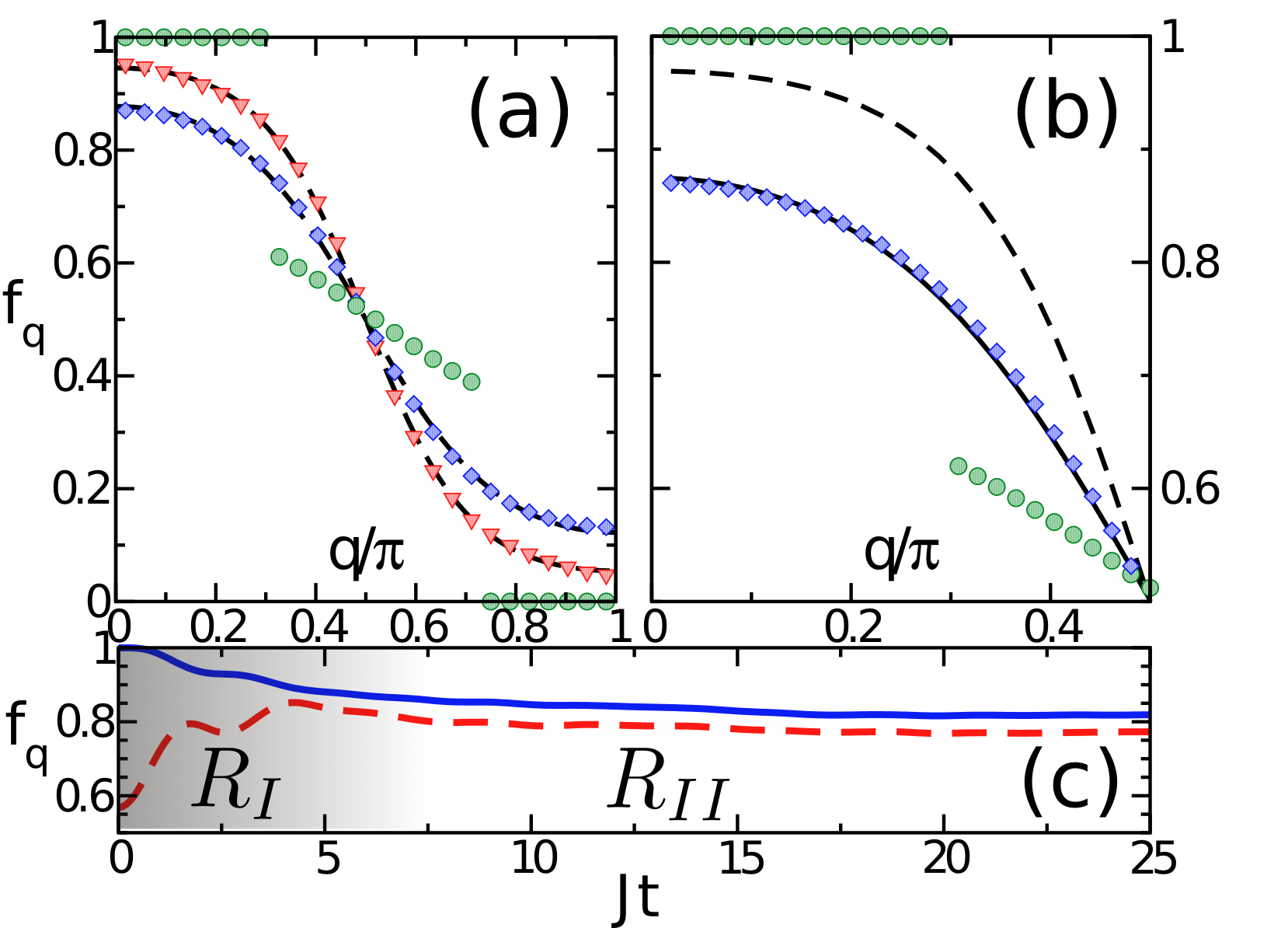
Figure 3: (Color online) (a) $f_{q}(t=0)$ for $|\Psi_{0}^{\textrm{II}}(1,0.6,1)\rangle$ (circles), $f_{q}(t=5)$ (triangles) and Fermi function fit $\langle f_{q}\rangle_{T=0.7J}$, and the extrapolated distribution $f_{q}(t\to\infty)$ (diamonds) with a fit $\langle f_{q}\rangle_{T=J}$. (b) $f_{q}(t\to\infty)$ (diamonds) compared to the thermal average $\operatorname{Tr}\{f_{q}\text{e}^{-H/T}\}/Z$ (solid line) and $\langle f_{q}\rangle_{T}$ (dashed line) where $T/J=0.54$ is fixed by Eq. (2). (c) $f_{q}(t)$ for $q=13\pi/52$ (solid line) and $q=16\pi/52$ (dashed line).

However, the system has not fully equilibrated yet. Fig. 3(c) shows that we have two distinct relaxation regimes. In regime $R_{I}$ we have a relatively quick reshuffling in the distribution leading to a prethermalized state Rigol et al. (2008); Gring et al. (2012). This is followed by a slow drift of the occupation numbers in regime $R_{II}$ which, when extrapolated in time, leads to the final distribution for the equilibrated state. While both distributions can be well fitted by $\langle f_{q}\rangle_{T}$, the temperature should not be used as a fitting parameter but should rather be determined by energy conservation. We therefore expect that the equilibrated system is described by the ensemble, $\rho=\exp(-H/T)/Z$, with the chemical potential $\mu=0$ due to particle–hole symmetry. The temperature T is determined by Eq. (2) with $\mathcal{Q}_{n}$ replaced by $H$. The lhs of Eq. (2) is now an expectation value for a noninteracting system and can be obtained analytically. The thermal average on the rhs is calculated using a static DMRG calculation Feiguin and White (2005). For the particular quench in Fig. 3 we find $T/J=0.54$. This then allows the calculation of $\langle C_{j}\rangle_{T}\equiv\operatorname{Tr}\{\hat{C}_{j}\text{e}^{-H/T}\}/Z$ by the DMRG algorithm as shown in Fig. 2. The results for the corresponding distribution function are shown as a solid line in Fig. 3(b) and agree well with the time extrapolated values, demonstrating a local thermalization.

If the additional sites are to represent an effective bath, the distribution function in the chain should become a Fermi distribution. However, as can be seen in Fig. 3(b), $\langle f_{q}\rangle_{T=0.54J}$ differs significantly from the equilibrium distribution. One obvious reason is that the effective coupling between the chain and bath in the thermal state $\sim\gamma\langle s^{\dagger}_{i}c_{i}\rangle_{T=0.54J}\approx 0.28\gamma$ is not small. Next, we therefore consider cases where we successively reduce the coupling $\gamma$. In order to be able to still find the equilibrated state within the limited simulation time we now use as the initial state $|\Psi_{0}^{\textrm{I}}(1,\gamma)\rangle$ which yields a much smoother initial distribution. Results for different coupling strengths $\gamma$ are shown in Fig. 4.

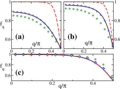
Figure 4: (Color online) The initial distribution (circles), $f_{q}(t\to\infty)$ from DMRG (diamonds), the thermal distribution $\operatorname{Tr}\{f_{q}\text{e}^{-H/T}\}/Z$ (solid line), and the free fermion distribution $\langle f_{q}\rangle_{T}$ (dashed line) with: (a) $\gamma=1$, $T/J=0.19$, (b) $\gamma=0.6$, $T/J=0.18$, and (c) $\gamma=0.2$, $T/J=0.33$.

We indeed find that the momentum distribution in equilibrium now approaches the free fermion distribution with the temperature determined by Eq. (2). At $\gamma=0.2$ the effective coupling between the chain and bath $\propto\gamma\langle s^{\dagger}_{i}c_{i}\rangle_{T=0.33J}\approx 0.06\gamma$ is very small. Apart from the usual Pauli blocking there is another mechanism which explains the very weak coupling between the subsystems. Because the nearest neighbor occupation $\langle n_{j}^{B}n_{j+1}^{B}\rangle_{T=0.33J}=0.1$ is also small we can approximately project out all states where nearest-neighbor sites in the bath are occupied. This leads to an effective density-density interaction $\propto(\gamma^{2}/V_{s})n_{j}^{A}n_{j}^{B}$ between the subsystems, leading to a slow relaxation for small $\gamma$ Sup . In this strong coupling limit, the hybridization part of the Hamiltonian Eq. (3) also gets projected $\propto\gamma(s^{\dagger}_{j}c_{j}+h.c.)(1-n_{j-1}^{B})(1-n_{j+1}^{B})$ explaining the small value for the effective coupling given above. Thus the interactions help to decouple the two subsystems explaining the almost perfect free Fermi distribution in the chain for $\gamma=0.2$.

Conclusions.

We have studied thermalization in a strongly correlated model which can be viewed either as a closed quantum system or as a free fermionic chain coupled to a bath. Contrary to the common approach of using a Lindblad equation to study open quantum systems, our model has a microscopically specified bath. Therefore we can simulate the nonequilibrium dynamics of the system and bath, and directly compare the two different viewpoints. For low particle densities we have shown that an equation of motion approach on the Hartree-Fock level is sufficient to quantitatively describe the intermediate time dynamics. At this level only slow dephasing processes are captured. For the future it seems promising to use a higher order decoupling which might also capture the faster relaxation processes which we observe in the numerical simulations. While the relaxation rate $\Gamma\sim V_{s}\langle n_{j}^{B}n_{j+1}^{B}\rangle$ at small interactions or low densities is too small to observe equilibration within the limited numerical simulation time we do observe thermalization at stronger interactions near half filing where $\Gamma$ is larger. We note that the relaxation rate changes continuously with the microscopic parameters of the model so that the definition of a ‘nonequilibrium phase transition’ based on the accessible simulation time $t_{\rm max}$ seems problematic Kollath et al. (2007). Most interestingly, we find that strong interactions lead to an effective disentanglement between the subsystems and therefore increase the decoherence times. Furthermore, even an extremely simple bath where Markovian dynamics cannot be taken for granted can be sufficient to fully equilibrate a subsystem without intrinsic relaxation processes.

Appendix A Equation of motion approach

We set up a set of equations for the following three time-dependent expectation values

$$f_{q}(t) = \langle\Psi(t)|c^{\dagger}_{q}c_{q}|\Psi(t)\rangle\;,$$

$$g_{q}(t) = \langle\Psi(t)|s^{\dagger}_{q}s_{q}|\Psi(t)\rangle\;\textrm{, and}$$ (6)

$$\rho_{q}(t) = \langle\Psi(t)|c^{\dagger}_{q}s_{q}|\Psi(t)\rangle\;.$$

Using Heisenberg’s equation of motion,

$$\dot{O}=\text{i}[H,O]\;,$$ (7)

with the Hamiltonian given by Eq. (1) of the main text and the standard fermionic commutation relations, one finds, with $n_{j}^{B}=s_{j}^{\dagger}s_{j}$,

$$\dot{f}_{q}(t) = 2\gamma R_{q}(t)\;,$$ (8)

$$\dot{g}_{q}(t) = -2\gamma R_{q}(t)+\frac{2V_{s}}{L+1}\sum_{i\neq j}\sin\left[qi\right]\sin\left[qj\right]\langle\Psi(t)|\left(s^{\dagger}_{i}s_{j}-s^{\dagger}_{j}s_{i}\right)\left[n^{B}_{j+1}\left(1-\delta_{i,j+1}\right)+n^{B}_{j-1}\left(1-\delta_{i,j-1}\right)\right]|\Psi(t)\rangle\;,$$

$$\text{i}\dot{\rho}_{q}(t) = \text{i}[\dot{r}_{q}(t)+\text{i}\dot{R}_{q}(t)]=-\left[\varepsilon_{q}+V_{s}\right]\rho_{q}(t)+\gamma\left[f_{q}(t)-g_{q}(t)\right]$$

$$+V_{s}\sqrt{\frac{2}{L+1}}\left[\sum_{j=1}^{L-1}\sin\left[qj\right]\langle\Psi(t)|c^{\dagger}_{q}s_{j}n^{B}_{j+1}|\Psi(t)\rangle+\sum_{j=2}^{L}\sin\left[qj\right]\langle\Psi(t)|c^{\dagger}_{q}s_{j}n^{B}_{j-1}|\Psi(t)\rangle\right]\;.$$

We have introduced the real functions $r_{q}(t)=\operatorname{Re}\rho_{q}(t)$ and $R_{q}(t)=\operatorname{Im}\rho_{q}(t)$. This set of coupled equations is exact.

To solve this set of equations we apply two approximations. Firstly a Hartree–Fock decoupling is used, i.e. we apply Wick’s theorem so that we have only two point correlation functions present, for example

$$\langle c^{\dagger}_{q}s_{j}n^{B}_{j-1}\rangle = \langle c^{\dagger}_{q}s_{j}\rangle\langle n^{B}_{j-1}\rangle-\langle c^{\dagger}_{q}s_{j-1}\rangle\langle s^{\dagger}_{j-1}s_{j}\rangle\;.$$ (9)

One should note that, amongst other effects, this approximation leaves

$$\dot{g}_{q}(t) = -2\gamma R_{q}(t)=-\dot{f}_{q}(t)$$ (10)

and hence $g_{q}(t)+f_{q}(t)\equiv N_{q}$ becomes independent of time. Therefore, by performing the Hartree–Fock decoupling, we lose all relaxation processes which can reshuffle the occupation of the momenta. Nonetheless, as demonstrated in Fig. 1 of the main text, for small densities this approximation is sufficient to get good quantitative agreement with DMRG calculations for intermediate times. The second approximation is “instantaneous dephasing”, which means that all off-diagonal elements of $\langle\Psi(t)|c^{\dagger}_{q}c_{k}|\Psi(t)\rangle$, etc., are taken to ‘instantaneously dephase’ and we keep only diagonal terms. For a periodic system this would be guaranteed by translational invariance, here it amounts to disregarding finite size effects from the boundaries. This means that all two point correlation functions are diagonal in momentum space. Following this we have

$$\dot{f}_{q}(t) = -\dot{g}_{q}(t)=2\gamma R_{q}(t)\;,\quad\dot{r}_{q}(t)=B_{q}(t)R_{q}(t)\;,$$

$$\dot{R}_{q}(t) = -\gamma[f_{q}(t)-g_{q}(t)]-B_{q}(t)r_{q}(t)\;,$$ (11)

with

$$B_{q}(t) = \frac{2V_{s}}{L+1}\bigg{[}\cos^{2}\left[q\right]g_{\pi-q}(t)-\sin^{2}\left[q\right]g_{q}(t)$$

$$+\sum_{k}\left(1-\cos\left[k\right]\cos\left[q\right]\right)g_{k}(t)\bigg{]}-V_{s}-\varepsilon_{q}\;.$$

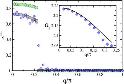
Figure 5: Main: A quench with initial state $|\Psi_{0}^{\textrm{I}}(1,1)\rangle$, and Hamiltonian $H$ with $J=1$, $\gamma=1$, and $V_{s}=1$ at low densities. Shown is $f_{q}(t=0)$ (circles), $\bar{f}_{q}$ within Hartree–Fock (squares), and $\bar{f}_{q}$ obtained by DMRG (diamonds). Inset: $\Omega_{q}$ obtained by DMRG (symbols) and within Hartree–Fock (line).

The coupled first order differential equations, given by Eq. (A), can then be solved iteratively. The first line in Eq. (A) is a $\mathcal{O}(1/L)$ finite size correction.

The oscillation frequency of $R_{q}(t)$ is the same as that of $f_{q}(t)$ and $g_{q}(t)$ and can be extracted from these equations analytically. We can write a second order differential equation for $R_{q}(t)$:

$$\ddot{R}_{q}(t)+\left(4\gamma^{2}+B_{q}^{2}(t)\right)R_{q}(t) = -\dot{B}_{q}(t)r_{q}(t)\;.$$ (13)

One finds, with a weakly time dependent bath occupation, such that $\dot{B}_{q}\approx 0$,

$$\ddot{R}_{q}(t)+\underbrace{\left(4\gamma^{2}+B_{q}^{2}(t)\right)}_{\equiv\Omega_{q}^{2}}R_{q}(t) = 0\;.$$ (14)

For small particle densities in the bath we can approximate $B_{q}(t)\approx-V_{s}-\varepsilon_{q}\equiv\mathcal{B}_{q}$ which gives

$$\Omega_{q}\approx\sqrt{(\varepsilon_{q}+V_{s})^{2}+4\gamma^{2}}\;.$$ (15)

The Hartree–Fock decoupled solutions oscillate with the frequency $\Omega_{q}$ which is only weakly $q$–dependent, see inset of Fig. 5. This explains why no dephasing effects are seen in the Hartree–Fock solution on the timescales that we consider, see Fig. 1 in the main text. The approximation $B_{q}(t)\approx\mathcal{B}_{q}$ is ensured in our case by the small bath occupation. For example, in the initial state $|\Psi_{0}^{\textrm{I}}(1,1)\rangle$, at a density of $0.11$ particles per site, we have

$$\frac{1}{L+1}\sum_{q}g_{q}(t=0)=0.0344\ll|{\cal B}_{q}|$$ (16)

and

$$\frac{1}{L+1}\sum_{q}g_{q}(t=0)\cos q=0.0314\ll|{\cal B}_{q}|\,.$$ (17)

Contrary to the Hartree–Fock results, the DMRG data show an additional relaxation, see Fig. 1 of the main text. A signature of the beginning of this relaxation can also be seen in the long time mean of the distribution function, $\bar{f}_{q}$, see Fig. 5 which shows a redistribution of the occupation of quasi-momenta around the Fermi momentum. The low density relaxation rate $\Gamma\sim V_{s}\sum_{j}\langle n^{B}_{j}n^{B}_{j+1}\rangle/L$, however, is small so that we can not see full thermalization within the DMRG simulation time $t_{\textrm{max}}$.

Appendix B Particle–hole symmetry

We define $H^{\prime}$ as the Hamiltonian given by Eq. (1) in the main text, but with hopping in the bath included:

$$H^{\prime} = H-J^{\prime}\sum_{j=1}^{L-1}\left\{s_{j}^{\dagger}s_{j+1}+h.c.\right\}\;.$$ (18)

$H^{\prime}$, and therefore also all half–filled groundstates, has particle–hole symmetry. The Hamiltonian $H^{\prime}$ is invariant under the mapping

$${\cal T}_{\textrm{ph}}:\left\{\begin{array}[]{ccc}c_{j}&\to&(-1)^{j}c_{j}^{\dagger}\\ c_{j}^{\dagger}&\to&(-1)^{j}c_{j}\\ s_{j}&\to&(-1)^{j+1}s_{j}^{\dagger}\\ s_{j}^{\dagger}&\to&(-1)^{j+1}s_{j}\end{array}\right.$$ (23)

which exactly describes particle–hole inversion.

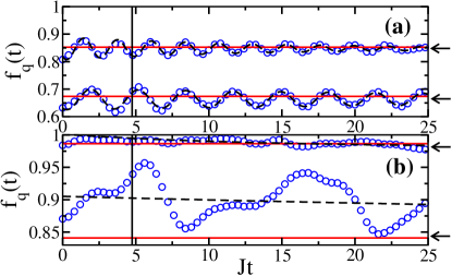
Figure 6: Momentum space extrapolation for a quench with initial state $|\Psi_{0}^{\textrm{I}}(1,\gamma)\rangle$, and Hamiltonian $H$ with $J=1$ and $V_{s}=1$ where (a) $\gamma=1$, and (b) $\gamma=0.2$. Shown are the momenta $q=11\pi/(L+1)$ (upper curves) and $q=21\pi/(L+1)$ (lower curves). The dynamics (symbols) are compared with the fit (dashed line), and the thermal average at the appropriate temperature (solid line). Fitting is performed for times greater than the solid vertical line. The arrows on the right hand side show $f_{q}(t\to\infty)$ from (a) Eq. (25), and (b) Eq. (26).

Figure 7: Real space extrapolation for a quench with initial state $|\Psi_{0}^{\textrm{II}}(1,0.6,1)\rangle$, and Hamiltonian $H$ with $J=1$, $\gamma=1$, and $V_{s}=1$. The DMRG data (symbols) are compared with the fit (dashed line), and the thermal average at the appropriate temperature (solid line). Plotted is $C_{j}(t)$ with (a) $j=1$, and (b) $j=3$. Fitting is performed for times greater than the solid vertical line. The arrows on the right hand side show $C_{j}(t\to\infty)$ from Eq. (27).

In our analysis we have considered two correlation functions. Firstly the real space two point correlation function $C_{j}(t)$, defined by

$$C_{j}(t)=\langle\Psi_{0}|e^{\text{i}Ht}c_{(L+1)/2}^{\dagger}c_{(L+1)/2+j}e^{-\text{i}Ht}|\Psi_{0}\rangle\;,$$ (24)

for time evolution with $H$ given by Eq. (1) in the main text. Under the mapping given by Eq. (23) $H\to H$ and $|\Psi_{0}\rangle\to|\Psi_{0}\rangle$ and one finds that $C_{j=0}(t)=1/2$, and $C_{2j}(t)=0$ for non–zero $j$. Secondly we analyzed the momentum distribution in the chain, $f_{q}(t)$. For the initial states under consideration, and therefore for all times, this can be shown to satisfy $f_{q}(t)+f_{\pi-q}(t)=1$ by using the same mapping.

Appendix C Fitting and extrapolation

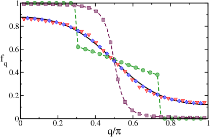
Figure 8: Distribution function $f_{q}$ in the chain for a system of size $L=51$. $f_{q}(t=0)$ is shown for the initial state $|\Psi_{0}^{\textrm{II}}(1,0.6,1)\rangle$ (circles), and the initial state $|\Psi_{0}^{\textrm{I}}(4.48,0.8)\rangle$ (squares). In both cases we time evolve with the same Hamiltonian $H$ with $J=1$, $\gamma=1$, and $V_{s}=1$. $f_{q}(t\to\infty)$ after time evolving $|\Psi_{0}^{II}\rangle$ (diamonds) and $|\Psi_{0}^{II}\rangle$ (triangles) are compared with the thermal average $\operatorname{Tr}\{f_{q}\text{e}^{-H/T}\}/Z$ (solid line) where $T/J=0.54$ is fixed by the initial energy, see text. Alternate $q$ points are plotted for the two quenches to aid clarity.

In this section we explain the fitting and extrapolation techniques we used to find our long time data at half–filling. For quench I we extrapolated in momentum space. The long time limit for $f_{q}$ and $\gamma=1$ and $\gamma=0.6$ can be found directly by time averaging the data or by fitting to

$$f_{q}(Jt\gg 1)\simeq f_{q}(t\to\infty)+ae^{-\Gamma t}\cos\left[\Omega t-\phi\right]\,.$$ (25)

This functional form takes into account exponential relaxation and a simple oscillation, see Fig. 6(a). Note that the fitting is only performed right of the solid line at $Jt\approx 5$, to ignore the effect of the short time dynamics. A Fourier analysis confirms that there is one dominant frequency in the dynamics of $f_{q}(t)$. However, in contrast to the low density case this frequency is momentum dependent. In particular for the case $\gamma=1$ shown in Fig. 6(a), $\Omega(q=11\pi/(L+1))\approx 2.7$ and $\Omega(q=21\pi/(L+1))\approx 1.9$. The relaxation rate, $\Gamma(q=11\pi/(L+1))\approx 6.7\cdot 10^{-2}$ and $\Gamma(q=21\pi/(L+1))\approx 2.7\cdot 10^{-2}$, is of the same order of magnitude for all momenta hinting at one dominant relaxation process. Let us stress that in this case the result for $f_{q}(t\to\infty)$ depends only weakly on the extrapolation procedure used, i.e. time averaging or fitting with different fit intervals, with a variation in $f_{q}(t\to\infty)$ which is about the symbol size used in the corresponding plots in the main text.

For $\gamma=0.2$, see Fig. 6(b), such a simple fitting function will no longer work due to the presence of various oscillation frequencies. A Fourier analysis confirms that there is more than one oscillation frequency involved, but the times are not sufficient to extract how many there are and what their magnitudes may be. Instead we trace out the overall trend by fitting to

$$f_{q}(Jt\gg 1)\simeq f_{q}(t\to\infty)+ae^{-\tilde{\Gamma}t}\,.$$ (26)

$\tilde{\Gamma}$ captures the gradual drift of the oscillations which can also be seen by using running averages. This procedure is robust when choosing a variety of different time regions over which to perform the fitting, and gives again errors smaller than the symbol sizes used in the plots of the main text.

For quench II we extrapolate in real space. Fig. 7 shows the fitting for $C_{1}(t)$ and $C_{3}(t)$. We fit the dynamics with

$$C_{j}(Jt\gg 1)\simeq C_{j}(t\to\infty)+ae^{-\Gamma t}\left(\cos\left[\Omega t-\phi\right]+b\right).$$ (27)

As for quench I, only times right of the vertical lines in Fig. 7 are used for fitting.

Appendix D Initial state independence

After relaxation the equilibrium state should depend only on the energy in the system. As example, we take two initial states, $|\Psi_{0}^{\textrm{I}}\rangle$ and $|\Psi_{0}^{\textrm{II}}\rangle$, constructed to have the same energy after a quench

$$E = \langle\Psi^{\textrm{II}}_{0}|H|\Psi^{\textrm{II}}_{0}\rangle=\langle\Psi^{\textrm{I}}_{0}|H|\Psi^{\textrm{I}}_{0}\rangle\,.$$ (28)

The two different initial states are time evolved with the same Hamiltonian, with $J=1$, $\gamma=1$, and $V_{s}=1$. We use the initial states $|\Psi_{0}^{\textrm{II}}(1,0.6,1)\rangle$ (same as in Fig. 3 of the main text) and $|\Psi_{0}^{\textrm{I}}(4.48,0.8)\rangle$ with energy $E=-51.19$. Fig. 8 demonstrates that both states evolve towards the same equilibrium state, well described by the grand canonical ensemble $\operatorname{Tr}\{f_{q}\text{e}^{-H/T}\}/Z$ with the temperature $T/J=0.54$ fixed by $E=\operatorname{Tr}\{H\text{e}^{-H/T}\}/Z$ and $\mu=0$ due to particle-hole symmetry.