Identification of the primary mass of inclined cosmic ray showers from depth of maximum and number of muons parameters

Abstract

In the present work we carry out a study of the high energy cosmic rays mass identification capabilities of a hybrid detector employing both fluorescence telescopes and particle detectors at ground using simulated data. It involves the analysis of extensive showers with zenith angles above 60 degrees making use of the joint distribution of the depth of maximum and muon size at ground level as mass discriminating parameters. The correlation and sensitivity to the primary mass are investigated. Two different techniques - clustering algorithms and neural networks - are adopted to classify the mass identity on an event-by-event basis. Typical results for the achieved performance of identification are reported and discussed. The analysis can be extended in a very straightforward way to vertical showers or can be complemented with additional discriminating observables coming from different types of detectors.

capbtabboxtable[][]

1 Introduction

Mass composition analysis is fundamental to understand the features observed in the cosmic ray energy spectrum and to test theoretical models concerning the origin and the nature of the primary cosmic ray radiation at the highest energies. Current theories predict different spectra for each mass component so that the knowledge of the energy spectra for every mass component, or at least for groups of components, is required in order to discriminate among the proposed models.
At low energies ($E<10^{14}$ eV) cosmic ray composition can be measured using direct detection techniques, such as spectrometers and calorimeters.
At higher energies, mass measurements are performed with indirect techniques, which make use of shower parameters sensitive to the primary mass. The depth at which the longitudinal development has its maximum, $X_{\mathrm{max}}$, and both the number of electrons $N_{e}$ and muons $N_{\mu}$ at ground level are most widely used. An extensive review of the adopted detection techniques and mass composition results over the entire energy spectrum range is presented in [1].
Two kinds of approaches are generally adopted in composition analysis. Likelihood methods, for instance in [2] or unfolding analyses, as in [3], aim to infer the average mass abundances or the energy spectra for different mass components on the basis of a set of parameters sensitive to the primary mass, without attempting to establish the mass of each single event. The information of the mass identity on an event-by-event basis would however be extremely useful and would lead to considerable progress. For instance when studying possible correlations of the shower arrival direction with given astrophysical objects it is desirable to select events according to their mass. Some worthwhile studies concern the flux of a given primary, e.g. protons for the p-Air cross section analysis or the search of gamma ray or neutrino events in the hadronic background. In all these situations pattern recognition methods, e.g. neural networks as in [4, 5], linear discriminant analysis [6], are typically employed.
Due to the absence of features strongly correlated to the mass and the presence of stochastic shower-to-shower fluctuations, both analyses must necessarily deal with a limited number of mass groups, typically four or five in first kind of analysis and two or three in event-by-event studies.
In this work we study the possibility to use neural networks and clustering algorithms as mass classifier tools on the basis of two parameters, the depth of shower maximum and the number of muons, measured with hybrid detectors, such as the Pierre Auger Observatory [7] or the Telescope Array [8]. In particular we restrict the analysis to events measured with very high zenith angles ($>$60^∘) at energies above $10^{18}$ eV. For such inclined showers the electromagnetic component is strongly absorbed before reaching ground level due to the large atmospheric depth traversed and the muon component dominates the signal measured at the particle detectors. To a rough approximation only the muon reaches ground level. These events therefore represent a simple way to measure a parameter reflecting the size of the muon component in experiments not equipped with dedicated muon detectors. This is achieved, as detailed in [9], by fitting the measured signals (after subtracting a small contribution due to the electromagnetic contamination) to a reference parameterization of the muon density at ground level obtained from simulations. The depth of maximum can be determined from the longitudinal profile extracted from the light measurements made with the fluorescence telescopes (see for instance [10]).
The paper is organized as follows. Section 2 describes the data set used for this study, built from Conex simulations of extensive air showers, and addresses the correlation between the two parameters ($X_{\mathrm{max}}$ and muon size) and the sensitivity to the primary mass. In Section 3 a brief description of the designed neural network and clustering methods is reported. In Section 4 their application to samples of simulated data and the achieved classification results are presented. Our main conclusions are summarized in Section 5.

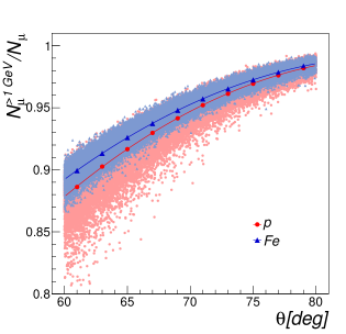
(a) $N_{\mu}$ correction factor

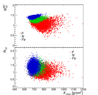
(b) $X_{\mathrm{max}}$-$N_{19}$

Figure 1: Fig. 1(a): $N_{\mu}$ correction factor for proton (in red) and iron (in blue) Aires simulations. Fig. 1(b): Scatter plot of the $X_{\mathrm{max}}$-$N_{19}$ parameters for proton (red), nitrogen (green) and iron (blue). The bottom panel refers to the case of detector resolution applied.

2 Simulated data

2.1 Simulation strategy

The present study is based on a sample of simulated showers generated with the Conex tool [11, 12] using Qgsjet01 [13] as high energy hadronic interaction model. Conex is an hybrid code, based on the combination of a Monte Carlo strategy and the analytic solution of the cascade equations, thus allowing only a one-dimensional simulation of the shower. It requires considerably shorter CPU times with respect to the ones needed by typical three-dimensional codes, such as Corsika [14] or Aires [15]. This feature makes Conex particularly suitable for applications involving data observed with fluorescence detector telescopes.
Proton, nitrogen and iron primaries have been simulated according to a flat energy spectrum from $10^{18}$ eV to $10^{20}$ eV and a $dN/(d\cos\theta)\propto\cos\theta$ zenith angle spectrum from 60^∘ to 80^∘. About 10⁶ events are available per each primary nucleus.
In order to perform a composition study, a set of parameters sensitive to the primary mass is needed. In this work we assumed the depth of shower maximum $X_{\mathrm{max}}$ and an estimator of the total number of muons $N_{\mu}$ reaching ground level for inclined showers, denoted as $N_{19}$. While $X_{\mathrm{max}}$ is directly available in Conex simulations, the latter has to be extracted from the simulated muon profile assuming a given observation depth. For our analysis we fixed such depth to 1450 m, roughly corresponding to the altitude of the Pierre Auger Observatory.
Unfortunately Conex provides the muon profile only for muons above 1 GeV, therefore we need to employ full Aires simulations to derive an empirical correction factor to be applied to $N_{\mu}$. In Fig. 1(a) we display the ratio between the number of muons above 1 GeV $N_{\mu}^{>1GeV}$ and the total number of muons $N_{\mu}$ as a function of the shower zenith angle. Proton results are shown in red dots while iron in blue triangles. As one can see the effect of the muon energy cut is not particularly relevant for inclined showers. The fraction of unaccounted muons is below 10% muons when using Conex. An empirical parameterization as a function of the zenith angle is derived and shown in Fig. 1(a) with solid colored lines . After this correction the simulated $N_{\mu}$ is divided by the number of muons of the reference parameterization of the muon density at ground, obtained for this location at a conventional energy of $10^{19}$ eV [9], to obtain the relative muon size with respect to the reference energy, $N_{19}^{MC}$. As the number of muons in the reference parameterization depends on the zenith angle, an estimator $N_{19}^{MC}$ is obtained which is basically independent of the zenith angle.
To take into account the reconstruction effects, the simulated ${X_{\mathrm{max}}}^{MC}$ and $N_{19}^{MC}$ have been smeared with the detector resolution. In this work we assume the resolution reported by the Pierre Auger Observatory in [9, 16]. Typical values for $\sigma_{{X_{\mathrm{max}}}}$ are $\sim$27 g/cm² at 10¹⁸ eV improving at $<$20 g/cm² above 10¹⁹ eV. The detector resolution $\sigma_{N_{19}}$ has been found of the order of 25% at 10^18.5 eV improving at $\sim$12% above 10¹⁹ eV. In Fig. 1(b) we present a scatter plot of $X_{\mathrm{max}}$ and $N_{19}$ at a fixed energy of 10¹⁹ eV for the three available primaries with the upper (lower) panel ignoring (accounting for) detector resolution as modelled.

2.2 Correlation of the parameters and sensitivity to primary mass

It is worth investigating the correlation of the two parameters and evaluating an estimator of the mass sensitivity for both. This has been studied in detail for vertical showers in [17]. Here we report the results obtained for inclined showers.
In Fig. 1(c) we report the Pearson correlation coefficient of both parameters for the three available nuclei,

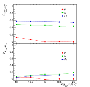
(c) ${X_{\mathrm{max}}}-N_{19}$ correlation

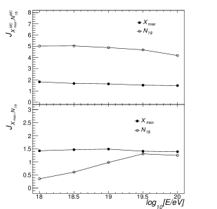
(d) ${X_{\mathrm{max}}}-N_{19}$ Fisher factor

Figure 2: Fig. 1(c): Correlation coefficient of ${X_{\mathrm{max}}}$-$N_{19}$ as a function of the primary energy for proton (red), nitrogen (green) and iron (blue). Fig. 1(d): Fisher coefficient of the ${X_{\mathrm{max}}}$ and $N_{19}$ parameters with respect to proton and iron primaries. Bottom panels take into consideration detector resolution effects.

the bottom panel accounting for detector resolution. As can be seen the two parameters are almost independent for proton primaries while for heavier nuclei the correlation amounts to 0.5 for nitrogen and 0.6 for iron. In the bottom panel the effect of the detector resolution is visible and the correlation observed for nuclei is sensibly reduced.
To estimate which of the two parameters offers the best separation between the proton and iron distribution we computed the Fisher coefficient $J$ for ${X_{\mathrm{max}}}$ and $N_{19}$:

$$J_{j}=\frac{(m_{j}^{Fe}-m_{j}^{p})^{2}}{[\sigma_{j}^{Fe}]^{2}+[\sigma_{j}^{p}]^{2}}\;\;\;\;\;j={X_{\mathrm{max}}},N_{19}$$ (1)

where $m_{j}$ and $\sigma_{j}^{2}$ are the sample mean and variance of the proton/iron distributions of the parameter $j$. The computed quantity provides a measure of power to separate two populations of proton and iron: large values of $J$ correspond to a good discrimination power. In Fig. 1(d) we report the Fisher coefficient as a function of energy. As can be seen the number of muons estimator has a better discrimination power than ${X_{\mathrm{max}}}$. However, the reconstruction of the ${X_{\mathrm{max}}}$ parameter, especially at low energies, is much better than that of $N_{19}$. This results in the increased sensitivity of ${X_{\mathrm{max}}}$ when applying the resolution to the data in the bottom panel. At the highest energies both parameters are almost equally powerful.

3 Analysis method

Two different classification methods are used in this work, one based on the neural network technique and the other on clustering algorithms. In the following sections we briefly describe the two approaches and the strategies adopted to perform the analysis.

3.1 The Clustering approach

A simple clustering algorithm, the well-known k-Means [18], is employed for the classification task. It starts assuming an initial set of $K$ cluster centroids, which are then iteratively moved to determine the partition of the data that minimizes a specified square error function $E^{2}$. We assumed the Euclidean distance as measure and the following squared error function:

$$E^{2}=\sum_{k=1}^{K}\sum_{j=1}^{n_{k}}\sum_{i=1}^{N}(\mathbf{x}_{ij}-c_{ik})^{2}$$ (2)

where $x_{ij}$ is the $i_{th}$ data vector (j=${X_{\mathrm{max}}}$,$N_{19}$) and $c_{ik}$ are the coordinates of the $K$ cluster centroids.
The data sample were first preprocessed to have zero mean and unit variance and then divided into three smaller subsets. One of these subsets is used for the cluster training phase in which the $K$ clusters determined are labelled on the basis of the Monte Carlo information of the primary mass. The validation subsets are mainly used to choose the optimal number of clusters, while the last subset if finally used to test the partition and report the performance of the method. As such algorithm is known to depend on the initial choice of the centroids, the algorithm was run over the three subsets assuming each time 100 different initial partitions and retaining the best one in terms of the total error. A number of clusters $K\geq$ 20 has been found to provide optimal results for our classification problem.

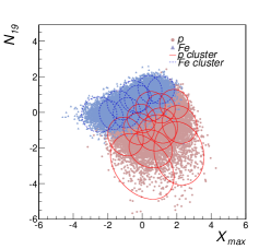
(e) Clustering output

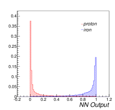
(f) NN output

Figure 3: 1(e): Clustering output projected in the ${X_{\mathrm{max}}}$-$N_{19}$ plane. Proton data are shown with red dots while iron data with blue triangles. The ellipses represent the obtained clusters (K=20): proton-labelled clusters (red solid lines), iron-labelled clusters (blue dashed lines). Data have been standardized in the plot; 1(f): Distribution of neural network outputs in presence of two components, proton (red histogram) and iron (blue histogram), for the test data sample. A sample energy bin corresponding to $\log_{10}$E=[19.0-19.2] is chosen.

3.2 The Neural Network approach

A feed forward neural network (NN) is structured in parallel layers of neurons, connected to neurons in adjacent layers through weighted links. The input layer is connected to the input data vector and a predefined number of hidden layers process the signal towards the output layer which returns the final response of the network to the presented input data. Each neuron $i$ linearly transforms the data $x_{j}$ from neurons in the previous layer according to the following expression:

$$z_{i}=\sum_{j=1}^{m}w_{ij}x_{j}+b_{i}$$ (3)

where $w_{ij}$ are the weights associated to the $j$ link and $b_{i}$ is an additive bias. The neuron output is then obtained by applying a transfer function $f(z_{i})$ to the neuron input $z_{i}$.
During the training phase the network weights and biases are iteratively adjusted to minimize the following error function $E_{\textsc{mse}}$:

$$E_{\textsc{mse}}=\frac{1}{2}\sum_{i=1}^{N}[y_{i}(\textbf{x},\textbf{w})-t_{i}]^{2}$$ (4)

defined as the sum of squared differences between the desired output $y_{i}$ and the computed network output $t_{i}$. To improve the network generalization capabilities a regularization term is often added to the above error function to minimize the squared sum of the network weights:

$$E_{\textsc{mse}}^{\textsc{reg}}=\gamma\,E_{\textsc{mse}}+(1-\gamma)\sum_{i=1}^{N_{W}}w_{i}^{2}$$ (5)

where $N_{W}$ are the number of weights of the network and $\gamma$ is a parameter responsible to guarantee a compromise between the network error minimization and the generalization performances of the network.
After testing several network architectures and choices of transfer functions, we obtained good results using a simple network design with one hidden layer (3 neurons), and an output layer with one neuron. The activation functions are hyperbolic tangent in the hidden layer and linear in the output layer.
The network input data have been normalized to zero mean and unit variance and then divided into three subsets, train-validation-test samples. The first is used to train the network. The cross validation sample is used to stop the training at a given epoch to avoid over fitting the data sample used for learning. The last sample is finally used to test the trained network identification capabilities.
Several back propagation training algorithms have been tested (steepest descent, conjugated gradient and quasi-Newton algorithms). We achieved better identification performances with quasi-Newton methods using the Broyden-Fletcher-Goldfarb-Shanno (BFGS) error minimization formula [19, 20].

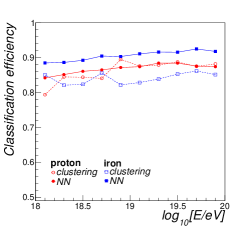
(g) Efficiency

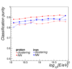
(h) Purity

Figure 4: Classification efficiency (left panel) and purity (right panel) for proton and iron events shown respectively with red dots and blue squares. Results relative to the clustering method are shown with empty markers while those obtained with the neural network with filled markers.

4 Results

The classification results obtained both with the clustering and the neural network methods are reported in Figs. 1(e) and 1(f) in a sample energy range $\log_{10}$E= [19-19.2].
In Fig. 1(e) we report the output of the clustering procedure for the test data sample projected in the ${X_{\mathrm{max}}}$-$N_{19}$ plane. Proton data are shown with red dots, while iron data with blue triangles. A number of K=20 clusters, represented by the ellipses, is considered for this case. A standard representation is adopted to visualize the obtained clusters. First a principal component analysis is applied to the standardized data to project data in the bidimensional space of the two most important components. The cluster ellipse’s axes are then defined by the eigenvalues of the covariance matrix of the observations belonging to that cluster. Finally the axes are scaled to create a 95% confidence ellipse. The achieved classification performances in terms of efficiency and purity are larger than 80% and are reported in Table 1.
In Fig. 1(f) we report the distribution of the network outputs in presence of the proton (red lines) and iron (blue lines) test data. The performance in terms of classification matrix and purity relative to such case are reported in Table 2. Assuming a cut in the network output equal to 0.5, the classification efficiencies and purity are found to be around 90%.

	Classification		Purity
	p	Fe
p	0.84	0.10	0.91
Fe	0.16	0.90	0.88

Table 1: Classification matrix and purity for the clustering method for the sample test data in the energy bin $\log_{10}E$= [19.0,19.2].

In Fig. 4 we report the classification efficiency for proton and iron (left panel) and the purity (right panel) as a function of the primary energy. Results obtained with the neural network (clustering) classifier are shown with filled (empty) dots. Both methods are able to accurately discriminate the two presented classes over the entire data set. The neural network method performs slightly better than the clustering approach. As expected, the classification performances are found to slightly increase with energy due to the improved reconstruction resolution for both ${X_{\mathrm{max}}}$ and $N_{19}$ parameters.

	Classification		Purity
	p	Fe
p	0.87	0.09	0.83
Fe	0.13	0.91	0.86

Table 2: Classification matrix and purity for the neural network method for the sample test data in the energy bin $\log_{10}E$= [19.0,19.2].

To have the smallest contamination for a given class and match a given analysis requirement one can tighten the applied selection cuts, increasing at the same time the event rejection rate, as shown in Figs. 3(a) and 3(c).

In Fig. 3(a) we report the classification efficiency (filled dots) and purity (empty dots) as a function of the network output for proton and iron data. The best compromise between the highest efficiency and purity is found around 0.55-0.60. To decrease the contamination from other species below few percent a cut of $\sim$0.2 for proton and $\sim$0.8 for iron must be assumed.
Similarly, for the clustering method a smaller contamination can be achieved by rejecting those clusters having a classification purity below a given requirement during the training phase. We therefore report in Fig. 3(c) the results as a function of the cluster purity obtained for the training data set. The steps observed in the plots are due to the fact that for a given purity threshold an entire set of events belonging to a cluster below threshold are rejected. The effect is more pronounced when a small number of clusters is assumed in the analysis.
The presented results so far assumed that no other species other than proton and iron is present in the flux. If an intermediate component, like nitrogen, is included in the data and both classifier are trained to recognize three species, the number of classifier parameters needed to achieve optimal results must be increased. The obtained performances deteriorate significantly in a 3-component situation.

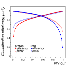
(a) NN - p+Fe data

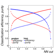
(b) NN - p+N+Fe data

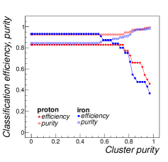
(c) Clustering - p+Fe data

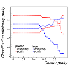
(d) Clustering - p+N+Fe data

Figure 5: Top panels: Classification efficiency (filled markers) and purity (empty markers) as a function of the cut applied in the neural network output. Proton and iron results are respectively shown with red dots and blue squares. Fig. 3(a) refers to a 2-components flux made by proton and iron, while in Fig. 3(b) nitrogen is added to the data sample; Bottom panels: Classification efficiency (filled markers) and purity (empty markers) as a function of the cluster purity for the clustering classifier method.

For the extreme components the identification efficiency and purity drops to a level of 75%, while for the intermediate component it is of order 60%. It is clear that with current parameter sensitivity to the mass and reconstruction resolution it is not possible to efficiently discriminate more than two masses. We therefore quantify in Figs. 3(b), 3(d) the increased contamination in the proton and iron classified samples due to the presence of nitrogen. For the neural network an optimal compromise is found assuming a cut equal to 0.2 and 0.8. The corresponding efficiency and purity are reduced at the 80% level. However one can obtain smaller contamination by further tightening the applied cuts at the cost of reducing the detection efficiency. For the clustering method the presence of an intermediate component rises the contamination in the proton and iron sample to values around 40-50%. To recover the contamination observed with proton and iron components only a large number of clusters must be rejected.

5 Summary

In the present work we propose two alternative strategies to the problem of the high energy cosmic ray mass identification on a event-by-event basis. One is based on the neural network technique while the other on clustering algorithms. The performances of both classifiers have been studied with simulated showers generated with the Conex tool. The mass discrimination is based on two parameters, the depth of shower maximum ${X_{\mathrm{max}}}$ and an estimator of the muon number $N_{19}$ reconstructed in very inclined showers. Realistic reconstruction resolutions have been assumed for both parameters. The analysis is in particular optimized for events recorded by hybrid detectors with zenith angles above 60^∘. Nevertheless it can be extended in a straightforward way to nearly vertical events, provided that an alternative muon number parameter estimator is introduced.
We have found very good identification performances for both methods in the case of a 2-component flux of proton and iron nuclei. The expected misclassification are found of the order of $\sim$10-15%, decreasing with energy, with slightly better performances exhibited by the neural network classifier.
A significant loss of efficiency is observed when training the classifiers to recognize a flux with an intermediate mass component added. In this situation the expected contamination affecting the proton and iron identification has been reported. No significant performance degradation has been observed with an alternative data sample generated using a different hadronic interaction model, such as Epos.
The present method, as it is, can be applied also to other typical discrimination problems in cosmic ray physics, such as hadron-gamma or hadron-neutrino event discrimination. In such cases the classification performances are expected to increase given the better separation between the two classes. Other feasible applications include the selection of a given mass group from the background, as it could be done for the selection of pure samples of protons for correlation analysis with astrophysical objects or to derive estimates of the proton-Air cross section.
In this work we made use of supervised methods. An implicit assumption is made, namely that the measured data must be well described or at least bracketed by the hadronic model predictions adopted in the classifiers. Surprisingly, this is the case for most of the shower observables so far measured at such extreme energies, i.e. see [1]. Furthermore, the differences among different models are going to be significantly reduced with incoming model releases accounting for recent LHC measurements, for instance see [21]. Recently a significant discrepancy between data and Monte Carlo simulations has been reported in the muon number estimator both for vertical [22] and for very inclined showers [9]. For this reason we are currently developing a semi-supervised classifier, partially using the strong constraints offered by the available models. Results and performance comparison with supervised methods will be reported in a forthcoming paper.

6 Acknowledgements

S. Riggi acknowledges the astroparticle group of the Universidad de Santiago de Compostela for support and ideas exchanging. We thank Xunta de Galicia (INCITE09 206 336 PR) and Consellería de Educación (Grupos de Referencia Competitivos – Consolider Xunta de Galicia 2006/51); Ministerio de Educación, Cultura y Deporte, Spain (FPA 2010-18410, FPA 2012-39489 and Consolider CPAN - Ingenio 2010) and Feder Funds. We are greatful to CESGA (Centro de SuperComputación de Galicia) for computing resources.

References

- [1] K.H. Kampert, M. Unger, Astroparticle Physics 35 (2012), 660.
- [2] D. D’Urso for the Pierre Auger Collaboration, Proc. of 31st International Cosmic Ray Conference (2009).
- [3] T. Antoni at al, Astroparticle Physycs 24 (2005) 1; W.D. Apel et al, Astroparticle Physics 31 (2009) 86.
- [4] A.K.O. Tiba, G.A.Medina-Tanco, S.J.Sciutto, astro-ph0502255.
- [5] M.Ambrosio et al, Astroparticle Physics 24 (2005) 355.
- [6] P. Abreu et al, Physical Review D 84 (2011) 122005.
- [7] J. Abraham et al, Nucl. Instr. Meth. A 523 (2004) 50.
- [8] T. Nonaka for the Telescope Array Collaboration, Proc. of 31st International Cosmic Ray Conference (2009); A. Taketa for the Telescope Array Collaboration, Proc. of 31st International Cosmic Ray Conference (2009); Y. Tameda et al, Nucl. Instr. Meth. A 609 (2009) 227.
- [9] G. Rodriguez for the Pierre Auger Collaboration, Proc. of 32nd International Cosmic Ray Conference (2011).
- [10] M. Unger, B.R. Dawson, R. Engel, F. Schussler and R. Ulrich, Nucl. Instr. Meth. A 588 (2008) 433.
- [11] T. Pierog et al, Nucl. Phys. B (Proc. Suppl.) 151 (2006) 159.
- [12] N.N. Kalmykov et al, Astroparticle Physics 26 (2007) 420.
- [13] N.N. Kalmykov et al, Nucl. Phys. B Proc. Suppl. 52 (1997) 17.
- [14] D. Heck, J. Knapp, J.N. Capdevielle, G. Schatz, T. Thouw, Forschungszentrum Karlsruhe Report FZKA 6019 (1998).
- [15] S.J. Sciutto, Proc. of 27th International Cosmic Ray Conference (2001).
- [16] J. Abraham et al, Phys. Rev. Letters 104 (2010) 091101.
- [17] P. Younk and M. Risse, Astroparticle Physics 35 (2012) 807.
- [18] J.A. Hartigan, M.A. Wong, Journal of the Royal Statistical Society C 28 (1979) 100.
- [19] C.M. Bishop, Neural Networks for Pattern Recognition, Oxford University Press (1995).
- [20] H. Demuth, M. Beale, Neural Network Toolbox - MATLAB - User’s Guide (2006), version 5.
- [21] T. Pierog, Proc. of 23rd European Cosmic Ray Symposium (2012).
- [22] J. Allen for the Pierre Auger Collaboration, Proc. of 32nd International Cosmic Ray Conference (2011).