SPECTRAL AND TIMING PROPERTIES OF THE MAGNETAR CXOU J164710.2$-$455216

Abstract

We report on spectral and timing properties of the magnetar CXOU J164710.2$-$455216 in the massive star cluster Westerlund 1. Using 11 archival observations obtained with Chandra and XMM-Newton over approximately 1000 days after the source’s 2006 outburst, we study the flux and spectral evolution of the source. We show that the hardness of the source, as quantified by hardness ratio, blackbody temperature or power-law photon index, shows a clear correlation with the 2–10 keV absorption-corrected flux and that the power-law component flux decayed faster than the blackbody component for the first $\sim$100 days. We also measure the timing properties of the source by analyzing data spanning approximately 2500 days. The measured period and period derivative are 10.610644(17) s (MJD 53999.06) and $<4\times 10^{-13}$ s s^-1 (90% confidence) which imply that the spin-inferred dipolar magnetic field of the source is less than $7\times 10^{13}\ \rm G$. This is significantly smaller than was suggested previously. We find evidence for a second flux increase, suggesting a second outburst between MJDs 55068 and 55832. Finally, based on a crustal cooling model, we find that the source’s cooling curve can be reproduced if we assume that the energy was deposited in the outer crust and that the temperature profile of the star right after the 2006 outburst was relatively independent of density.

1. Introduction

Neutron stars with ultrastrong magnetic fields, so-called magnetars, can emit radiation which is orders of magnitude stronger than their rotation power. These objects are prone to X-ray outbursts in which the flux rises rapidly then decays over days to months (see Woods & Thompson, 2006; Mereghetti, 2008; Rea & Esposito, 2011, for reviews). Such outbursts are often accompanied by short X-ray and soft gamma-ray bursts. The origins of outbursts are still debated. It has been suggested that a sudden or gradual internal heat release possibly caused by crustal cracking, heats the star from within, and induces observed temperature and luminosity increases (Thompson & Duncan, 1995, 1996; Perna & Pons, 2011). It has also been suggested that crustal motion can generate twists in the external magnetic fields (Thompson et al., 2002). The twisted magnetic fields induce currents in the magnetosphere, which return to the stellar surface and heat it.

The flux relaxation following an outburst can be explained as passive cooling of the hot star (Lyubarsky et al., 2002; Pons & Rea, 2012, see also Cumming et al. 2012, in preparation), or as “untwisting” of the external magnetic fields (Beloborodov, 2009). In either case, flux and spectral hardness are expected to be correlated (Thompson et al., 2002; Lyutikov, 2003; Özel & Güver, 2007). The correlation has been observed in many magnetars (e.g., SGR 1806$-$20, 1E 2259$+$586, 1E 1547$-$5408; Woods et al., 2007; Zhu et al., 2008; Scholz & Kaspi, 2011) although it is not as clearly seen in some sources (e.g., SGR 1900$+$14, SGR 1627$-$41; Tiengo et al., 2007; An et al., 2012).

Table 1Summary of observations and spectral fit results

#	Date	Observatory	Mode	ID	$kT$	$\Gamma$	BB radius	Flux	PL Flux	$\Delta T$
	MJD				(keV)		(km)			(s)
1	53513.0	Chandra	TE	6283	0.51(2)	$\cdots$	0.50(5)	0.030(2)	$\cdots$	3.24
2	53539.9	Chandra	TE	5411	0.53(14)	3.33(55)	0.25(13)	0.028(11)	0.02(1)	3.24
3	53995.1	XMM	FW/FW	0404340101	0.59(6)	3.86(22)	0.18(4)	0.025(4)	0.016(3)	2.6/0.073
4	54000.7	XMM	FW/FW	0311792001	0.70(1)	2.90(6)	1.44(5)	3.00(7)	1.62(6)	2.6/0.073
5	54005.4	Chandra	CC	6724	0.60(1)	2.46(13)	2.22(9)	2.52(9)	0.99(7)	0.00285
6	54010.1	Chandra	CC	6725	0.60(1)	2.69(12)	2.08(8)	2.08(7)	0.74(6)	0.00285
7	54017.4	Chandra	CC	6726	0.61(1)	2.92(13)	1.97(6)	1.84(6)	0.53(5)	0.00285
8	54036.4	Chandra	CC	8455	0.58(1)	2.78(17)	1.97(9)	1.42(6)	0.41(5)	0.00285
9	54133.9	Chandra	CC	8506	0.56(1)	2.86(18)	1.83(9)	0.95(4)	0.29(3)	0.00285
10	54148.5	XMM	SW/LW	0410580601	0.58(1)	3.20(11)	1.39(5)	0.78(2)	0.27(2)	0.3/0.048
11	54331.6	XMM	SW/LW	0505290201	0.58(1)	3.42(10)	0.99(4)	0.42(2)	0.17(1)	0.3/0.048
12	54511.5	XMM	SW/LW	0505290301	0.54(2)	3.40(14)	0.93(7)	0.26(1)	0.11(1)	0.3/0.048
13	54698.7	XMM	SW/LW	0555350101	0.57(2)	3.76(15)	0.62(4)	0.16(1)	0.068(8)	0.3/0.048
14	55067.6	XMM	SW/LW	0604380101	0.53(2)	3.68(15)	0.56(4)	0.087(5)	0.036(4)	0.3/0.048
15	55832.0	XMM	SW/LW	0679380501	0.73(1)	2.89(11)	0.67(3)	0.54(2)	0.18(2)	0.3/0.048
16	55857.8	Chandra	TE subarray	14360	0.62(2)	1.50(47)	0.87(8)	0.44(4)	0.18(2)	0.44

Notes. The outburst occurred on 53999.05659 (MJD). Obs. 3 (MJD 53995.1) was used to set the quiescent level for the flux evolution (Fig. 1). $N_{\rm H}$ was obtained by simultaneously fitting Obs. 4–14, and was fixed for fitting the others. Fits are conducted in the 0.5–10 keV band, and uncertainties are at the 1-$\sigma$ confidence level.
^a MOS1,2/PN for the XMM-Newton observations. TE: Timed Exposure, CC: Continuous clocking, FW: Full Window, LW: Large Window, SW: Small Window.
^b Blackbody radius. Results of tbabs(bbodyrad+pow) fitting in XSPEC for an assumed distance of 5 kpc.
^c Absorption-corrected flux in the 2–10 keV band in units of $10^{-11}$ erg cm^$-$2 s^$-$1.
^d Absorption-corrected power-law flux in the 2–10 keV band in units of $10^{-11}$ erg cm^$-$2 s^$-$1.
^e Time resolution.

The high magnetic fields of magnetars have been inferred both from spin-down rates, assuming the standard dipole braking relation $B\equiv 3.2\times 10^{19}(P\dot{P})^{1/2}\ \rm G$ (Manchester & Taylor, 1977), as well as from indirect arguments regarding radiative behavior and field decay (Thompson & Duncan, 1995, 1996). Indeed the typical magnetic field for an object classified as a magnetar on the basis of radiative behavior is $10^{14}-10^{15}$ G. However recently a small handful of objects have been reported to have fields below this range, overlapping with those of apparently ordinary radio pulsars (SGR 0418$+$5729, Swift J1822.3$-$1606; Rea et al., 2010; Livingstone et al., 2011; Rea et al., 2012; Scholz et al., 2012). Although the $B$-distribution of radiatively classified magnetars still remains significantly higher than that of radio pulsars (Livingstone et al., 2011), the apparently low-$B$ magnetars are puzzling and are suggestive of higher order multipolar structure or strong internal toroidal fields, for which the dipole component is deceptively low (Turolla et al., 2011).

CXOU J164710.2$-$455216 was discovered on 1998 June 15 with the Chandra X-Ray Observatory (Muno et al., 2006). It is located at R.A. = 16^h47^m10^s.20, Decl. = $-$45^∘52^′17^′′.05 (J2000.0, Skinner et al., 2006) and is estimated to be $2.5-5$ kpc away, in the massive star cluster Westerlund 1 (Clark et al., 2005). A short 20-ms burst was detected with the Swift Burst Alert Telescope (BAT) on 2006 Sept. 21 (MJD 53999.05659, Krimm et al., 2006). The source was subsequently observed with multiple X-ray observatories including Swift, XMM-Newton, Chandra and Suzaku. Israel et al. (2007) and Woods et al. (2011) reported on the data obtained after the 2006 outburst out to approximately 100–200 days and measured spectral and timing properties, where they concluded that there is no clear evidence of significant spectral variability. The pulsar’s spin period is $\sim 10.6$ s (Muno et al., 2006) and the spin-down rate has been reported to be $0.8-1.3\times 10^{-12}$ s s^$-$1 (Israel et al., 2007; Woods et al., 2011). These previously reported spin parameters imply an inferred surface dipolar magnetic-field strength of $B=0.95-1.2\times 10^{14}$ G.

Here, we report on the analysis of Chandra and XMM-Newton archival data which cover a longer time period ($\sim$2500 days). We study the long-term spectral evolution of the source after its outburst and report on the pulsar’s timing behavior during this period.

In Section 2, we summarize the observations we used for our study. We then describe our data analysis and results in Section 3, discuss the results in Section 4, and finally present our conclusions in Section 5.

2. Observations

Table 1 presents the data we used for our analysis. In total, we analyzed 16 observations obtained with the Chandra and XMM-Newton telescopes over the course of $\sim$2500 days. For the Chandra observations, we reprocessed the standard pipeline output using chandra_repro of CIAO 4.4 along with CALDB 4.4.7 to produce the “level 2” event lists using the newest software and calibration updates. For the XMM-Newton data, we processed the Observation Data Files (ODF) with epproc and emproc and then applied the standard filtering procedure (e.g., flare rejection and pattern selection) of Science Analysis System (SAS) version 11.0.0. Some observations in the Table were already analyzed by other authors (Muno et al., 2006, 2007; Israel et al., 2007; Woods et al., 2011). However, we re-analyzed those using the above procedure for consistency.

3. Data Analysis and Results

3.1. Imaging Analysis

We detected the source with wavdetect for the Chandra TE mode observations and with edetect_chain for the XMM-Newton observations. The source positions we found are all consistent with one another and with the known source location within 90% uncertainties of the position measurements (0^′′.6 for Chandra and 2^′′ for XMM-Newton).

The relatively large point-spread function of XMM-Newton was a concern since the source is located in a star cluster, and any other object within $\sim 30^{\prime\prime}$ could in principle contaminate the source spectrum. With two Chandra TE observations (IDs 6283 and 14360), we searched for X-ray sources within a radius of 30^′′ centered at CXOU J164710.2$-$455216 but found none. We also checked whether our source is consistent with being a point source using the eradial tool for XMM-Newton observations and Chandra Ray Tracer and the MARX tools for the Chandra observations. The data were consistent with the target being a point source in all the observations except for the first XMM-Newton observation (ID: 0311792001), where the radial profile of the source was distorted due to pile-up. Therefore, we conclude that there is no significant contamination from unresolved sources in the XMM-Newton observations and that the source exhibits no detectable extended emission.

3.2. Spectral Analysis

We used all the data listed in Table 1 for our spectral analysis. For the Chandra observations, we extracted the source events using a box of dimension 2^′′ along the 1-D events and 5^′′ in the orthogonal direction for the CC-mode observations, and a circle with radius $2^{\prime\prime}$ for the TE-mode observations. Backgrounds were obtained in two rectangular regions with size of $10^{\prime\prime}\times 5^{\prime\prime}$ from each side of the source region and an annular region with radii of 5^′′ and 10^′′ centered at the source for the CC-mode and the TE-mode observations, respectively. Then we produced spectra using the specextract tool of CIAO 4.4 with CALDB 4.4.7 and grouped them to have a minimum of 20 counts per bin for further analysis.

For the XMM-Newton data, we extracted source spectra from circular regions having radius of 16^′′ and background spectra from source-free regions on the same chip. Corresponding response files were produced using the rmfgen and the arfgen tasks of SAS 11.0.0. Each spectrum was then grouped to have a minimum of 20 counts per bin.

The first XMM-Newton observation was mildly piled up, so we excluded the central $\sim$5^′′ in each of the PN and the two MOS detectors to minimize the pile-up effect. After removing the central regions, we checked if pile-up was still significant using the epatplot tool of SAS. With the removal, the measured event pattern distributions showed good agreement with the expected ones. We also checked if the spectral parameters changed significantly when we removed central regions of different sizes. The power-law index changed smoothly by approximately 3% when we varied the removal radius from 0^′′ to 9^′′ for the PN data, but it changed abruptly (softened by 10%) for removal regions between 0^′′ and 3^′′.5 and then stayed constant for the MOS data. Therefore, we ignored the central 5^′′ for both the PN and the MOS data to ensure that pile-up would not distort the spectrum of the source in this one observation.

We fit the 0.5–10 keV spectra with three models: an absorbed power law plus blackbody, an absorbed double blackbody and an absorbed blackbody (tbabs*(power + bbody), tbabs*(bbody + bbody) and tbabs*bbody in XSPEC 12.7.0). We fit all the data in which the source flux decreased monotonically after the 2006 outburst (Obs. 4–14; see Table 1) simultaneously with a common hydrogen column density ($N_{\rm H}$).

The single blackbody fit ($\chi^{2}/DoF=9117.42/7062$) and double blackbody fit ($\chi^{2}/DoF=7353.82/7040$) were not acceptable as they showed systematic trends in the low energy ($<1$ keV) and the high energy bands ($>8$ keV). However, the blackbody plus power-law fit described the observed spectra well ($\chi^{2}/DoF=6988.04/7040$). The $N_{\rm H}$ we obtained from the fit is $2.39(5)\times 10^{22}$ cm^$-$2, which is different from the values that Muno et al. (2007, 1.44 $\times 10^{22}$ cm^$-$2) and Israel et al. (2007, 1.9 $\times 10^{22}$ cm^$-$2) used. However, it is consistent with that obtained by Woods et al. (2011) and that reported by Skinner et al. (2006, 2.1–3.0$\times 10^{22}$ cm^$-$2) on the basis of cluster extinction estimates of Clark et al. (2005) and the empirical relation of Gorenstein (1975). We then fixed $N_{\rm H}$ and tried to fit the spectra of the other, fainter observations with the same models. The results are summarized in Table 1.

We assumed that the source was in (or near) quiescence for the first three observations (Obs. 1–3). The source spectrum was well fitted with a single blackbody for Obs. 1 without requiring an additional component, although a power law was not ruled out unambiguously. We fit Obs. 2 and 3 with a power law; a single blackbody fit was unacceptable. However, adding another component (blackbody) significantly improved the fit (F-test probabilities of 0.048 and 0.00063 for Obs. 2 and 3, respectively).

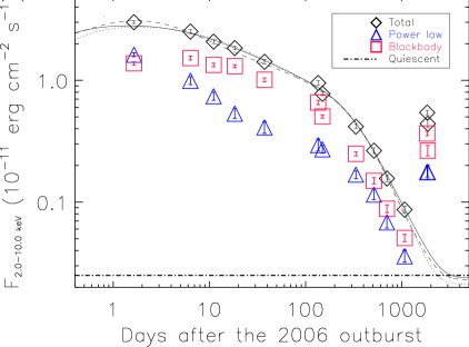
Figure 1.— Flux evolution of CXOU J164710.2$-$455216 after the 2006 outburst and crustal cooling model fits. Symbols are 2–10 keV absorption-corrected flux evolutions for total (diamonds), power-law (triangles) and blackbody (squares) components, and lines are quiescent flux (dot-dashed, Obs. 3 in Table 1) and crustal cooling models for decay of the source flux (see Section 4.2 for details). Solid line: $T_{c}=1.1\times 10^{8}\ \rm K$, $B=8\times 10^{13}\ \rm G$, $Q_{imp}=5$, initial temperature changes from $1.37\times 10^{9}\ \rm K$ at $9\times 10^{8}\ \rm g\ cm^{-3}$ to $4.5\times 10^{8}\ \rm K$ at $5\times 10^{11}\ \rm g\ cm^{-3}$. Dotted line: $T_{c}=9\times 10^{7}\ \rm K$, $B=2\times 10^{14}\ \rm G$, $Q_{imp}=1$, initial temperature changes from $1.3\times 10^{9}\ \rm K$ at $\rho=1\times 10^{9}\ \rm g\ cm^{-3}$ to $4\times 10^{8}\ \rm K$ at $\rho=5\times 10^{11}\ \rm g\ cm^{-3}$. Dashed line: $T_{c}=5.7\times 10^{7}\ \rm K$, $B=2\times 10^{15}\ \rm G$, $Q_{imp}=5$, initial temperature is $T=1.5\times 10^{9}\ \rm K$ for $1.5\times 10^{9}\ \rm g\ cm^{-3}<\rho<1\times 10^{11}\ \rm g\ cm^{-3}$. Other parameters were held fixed: $M=1.4M_{\sun}$, $R=12\ \rm km$. Note that the uncertainty for each data point is smaller than the symbol size.

Another flux increase was observed in Obs. 15, which might be due to a second outburst between MJDs 55068 and 55832 (see Fig. 1). We were not able to fit the spectrum for Obs. 15 or 16 with single-component models. For Obs. 15, a blackbody plus power law provided a better fit ($p=0.080$) than a double blackbody ($p=0.033$ for $kT_{1}=0.36(2)$ keV, $kT_{2}=0.82(2)$ keV). For Obs. 16, a double blackbody model fit the data better with $kT_{1}=0.58(3)$ keV and $kT_{2}=1.33(35)$ keV although a blackbody plus power law also provided an acceptable fit. Since it seems unlikely that the blackbody temperature increased from $0.80$ keV to $1.33$ keV without any accompanying flux increase, we report the blackbody plus power-law spectrum for Obs. 15 and 16. The results of all our spectral fits are reported in Table 1.

Figure 2.— The time evolution of various spectral properties. The top axis shows the 2–10 keV absorption-corrected flux interpolated with the double-exponential relaxation fit to the flux evolution (see section 3.3). The conversion between time and flux was obtained from the double exponential fit result. Clear trends in time (flux) are visible. a) Hardness ratio ($F_{4-10\ \rm keV}/F_{2-4\ \rm keV}$). b) Power-law photon index. c) Blackbody temperature. d) Blackbody radius assuming a distance of 5 kpc.

We also fitted the spectra for Obs. 3–14 with an absorbed resonant cyclotron scattering model, tbabs*(atable{RCS.mod}) in XSPEC (Rea et al., 2008). From the fit, we obtained a smaller $N_{\rm H}$ ($2.06\pm 0.02\times 10^{22}\ \rm cm^{-2}$), as expected because of the strong cutoff in the power-law spectrum at low energies. We were able to measure 2–10 keV absorption-corrected fluxes using the model, and they agreed well with those of the blackbody plus power-law fits described above. However, the RCS model parameters were not well constrained. Therefore, we mainly use the results of the blackbody plus power-law fit for discussion below.

3.3. Spectral Evolution

We plot the time evolution of the 2–10 keV absorption-corrected fluxes after the 2006 outburst in Figure 1. We have attempted to fit the data out to $\sim$1000 days with a double exponential, $F(t)=F_{1}e^{-(t-t_{0})/\tau_{1}}+F_{2}e^{-(t-t_{0})/\tau_{2}}+F_{Q}$ or a broken power law, $F(t)=F_{1}(t-t_{0})^{\alpha_{1}}+F_{Q}$ for $t_{0}<t<T_{break}$ and $F(t)=F_{2}(t-t_{0})^{\alpha_{2}}+F_{Q}$ for $T_{break}<t$, where $F_{1}$ and $F_{2}$ are determined so that $F(t)$ is continuous at $t=T_{break}$. In fitting, we set $t_{0}$ to be the onset of the outburst (MJD 53999.05659) and fixed the quiescent flux ($F_{Q}$) to be the measured value of $2.5\times 10^{-13}$ erg cm^$-$2 s^$-$1 (Obs. 3 in Table 1).

Although the fit results with the simple analytical models were statistically unacceptable, the double exponential function roughly described the relaxation with decay times of $18\pm 2$ and $325\pm 10$ days ($\chi^{2}$/dof=33.5/7), as did the broken power-law fit with decay indices of $-0.22\pm 0.01$ and $-1.16\pm 0.02$, and $T_{break}$ of $106\pm 5$ days ($\chi^{2}$/dof=64.8/7). Note that we include only statistical uncertainties in fitting, although some systematic for example, the sudden decrease in flux at $\sim$150 days in Figure 1 may indicate a cross-calibration issue between Chandra and XMM-Newton. Indeed, adding a 6% systematic uncertainty to the fluxes made the double exponential fit acceptable (decay times of $19\pm 4$ and $331\pm 15$ days, $\chi^{2}$/dof=12.3/7).

Table 2Timing properties of CXOU J164710.2$-$455216

	Period	Period Derivative	Epoch	$B$	Comment
	(s)	(s s$-$1)	(MJD)	($10^{14}$ G)
Israel et al. (2007)	10.6106549(2)	$9.2(4)\times 10^{-13}$	53999.0	1.00	$\cdots$
Woods et al. (2011)	10.6106567(1)	$8.3(2)\times 10^{-13}$	54008.0	0.95	$\cdots$
	10.6106567(2)	$1.3(1)\times 10^{-12}$		1.19	with cubic term
This work	10.610644(17)	$<4\times 10^{-13}$	53999.1	$<$0.7	$\cdots$

Notes. ^a Spin-inferred dipolar magnetic field.
^b 90% upper limit.

We also plot the time evolutions of the spectral properties for the same data in Figure 2 in order to look for any correlation between spectral hardness and flux, as seen in other magnetars (e.g., Rea et al., 2005; Woods et al., 2007; Campana et al., 2007; Tam et al., 2008; Zhu et al., 2008; Scholz & Kaspi, 2011). Clear trends are visible in the hardness ratio, power-law photon index and blackbody temperature; the spectrum clearly softened as the flux decreased.

For the first $\sim$100 days, we were able to reproduce the same trends as those of Woods et al. (2011) for the spectral parameters, though with small offsets within uncertainties in the power-law index and the blackbody temperature. The offsets could be due to the fact that they used a different CALDB or analysis software version and/or included a Suzaku observation.

3.4. Timing Analysis

Timing studies have been done by Israel et al. (2007) and Woods et al. (2011) using phase-coherent analyses with data obtained for approximately 100–200 days after the 2006 outburst. Since the separation between observations 10 and 11 was large, phase connection was lost. Instead, we searched for the best pulse period in each observation to find the average spin-down rate. To do this, we employed the $H$-test (de Jager et al., 1989) because it requires no advance knowledge of the pulse profile at any epoch, and because this source’s pulse profile is known to change (Israel et al., 2007; Woods et al., 2011).

The pulse period of the source is $\sim$10.6 s. The time resolutions of the observations are all smaller than $\sim$5 s so could be used in our analysis (see Table 1). Thus, the baseline useful for timing spans approximately 2500 days. We extracted source events from the regions described in Section 3.2. Then we selected events having energies in the range 0.5–8 keV for the analysis. Each observation was then corrected to the barycenter using the axbary tool of CIAO for the Chandra data and the barycen tool of SAS for the XMM-Newton data.

For each observation, we calculated the sum of the Fourier powers of $n$ harmonics, $Z_{n}^{2}(P)$ (Buccheri et al., 1983) for $n$=1–20 at test periods in the range 10.6050–10.6160 s with step size $\Delta P=10^{-5}$ s and found $n$ and $P$ which maximized $H=Z_{n}^{2}(P)-4n+4$ (de Jager et al., 1989) for each observation. We folded the events at the best period to obtain a pulse profile. We used simulations to determine the uncertainty on the best period. To do this, we used the measured pulse profiles (which had 40 bins) to produce fake event lists containing the periodicities. Fake event lists were made by first taking an observed pulse profile, and adding Poisson noise as well as a random phase offset to it. Then, for each bin in the profile, we took the total number of counts, assigned each one a random arrival time in that phase bin and rebinned the arrival times to the time resolution of the detector. In this way, we constructed a simulated event list. For each such list, we then calculated the $H$ statistics for each $P$ in the range given above, and for all $n$’s in the range of 1–20. We then found $P$ and $n$ that maximized $H$, and took the standard deviation of the periods as the period uncertainty. The uncertainties we obtained in this way agree with those calculated using the method of Ransom et al. (2002) within a factor of two, but typically are slightly larger. To run the simulations for observations with coarse time resolution where the measured pulse profiles were not well determined, we assumed the XMM PN profile.

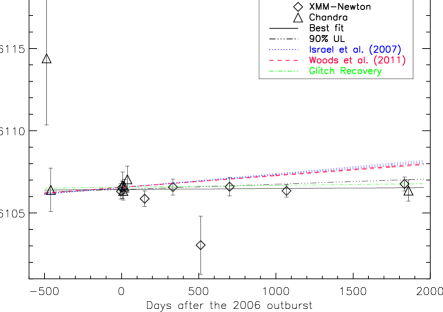
Figure 3.— The evolution of pulse period after the 2006 outburst. Periods are measured using the $H$-test (de Jager et al., 1989) and uncertainties are estimated using simulations (see text). The solid line is the best fit to the data, the triple dot-dashed line is the 90% upper limit for the best fit, and the dotted and the dashed lines are the expected evolution of the period in time for the previously reported period derivative with 90% confidence interval by Israel et al. (2007) and Woods et al. (2011) with no cubic term, respectively. Also plotted in the dot-dashed line is the solution of Woods et al. (2011) assuming glitch recovery following the 2006 outburst.

In Figure 3, we show the best period we obtained for each observation. For the XMM-Newton observations, we took the variance-weighted average period for measurements done with the three instruments (MOS1, MOS2 and PN). We then fit the periods with a linear function ($P(t)=P_{0}+\dot{P}t$) to obtain the best period at the time of outburst, $P_{0}$ and the spin-down rate. The fit results were $P_{0}=10.610644\pm 0.000017$ s and $\dot{P}=0.7\pm 2.4\times 10^{-13}$ s s^-1. The period derivative we measured is consistent with zero, so we report the 90% upper limit, $4\times 10^{-13}$ s s^-1. This is significantly smaller than what Israel et al. (2007) and Woods et al. (2011) reported (see Table 2, and Section 4.3 for discussion).

We also searched for short-term aperiodic variability of the source in the 0.5–8 keV band. For the XMM-Newton data, we produced light curves using evselect and corrected them for detection efficiency with the epiclccorr tool of SAS. We binned the light curves at 30 to 2000 s intervals (ensuring at least 20 events per bin) depending on the source flux since it was declining. We then fit the light curves to a constant, and calculated $\chi^{2}$ and the null hypothesis probability. For the Chandra CC-mode observations, it is difficult to correct the detection efficiency because they lack information on one of the two dimensions. Therefore, we assumed a uniform detection efficiency for the data taken with CC-mode. We then performed the $\chi^{2}$ test and the Gregory–Loredo test (using the glvary tool of CIAO; Gregory & Loredo, 1992) for all the Chandra observations in Table 1. In all cases, the observed light curves were consistent with being constant.

4. Discussion

We have measured the spectral and timing properties of CXOU J164710.2$-$455216 for three years after its 2006 outburst. We observe a clear correlation between spectral hardness and flux post-burst. In our timing analysis, we find a significantly smaller period derivative which implies a spin-inferred dipolar magnetic field of $<7\times 10^{13}\ \rm G$ (90% confidence). This is significantly lower than was previously reported. We find evidence that a second outburst occurred between MJDs 55068 and 55832 based on a flux increase at MJD 55832 (Obs. 15). Next we discuss our findings in relation to previous studies of this source, and in the context of the magnetar model.

4.1. Correlation between Spectral Hardness and Flux

The spectral evolution of the source after the 2006 outburst has been discussed in previous studies (Israel et al., 2007; Woods et al., 2011). Based on 100–200 days of observations, Israel et al. (2007) and Woods et al. (2011) found no clear evidence that the spectral shape ($kT$ and $\Gamma$) had evolved. Our analysis results for the same period qualitatively agree with theirs (see the first seven data points of the $\Gamma$ and $kT$ evolution plots in Figure 2).

However, the power-law photon index may not be a reliable measure of spectral hardness because a power law may not be the true spectrum, especially at low energies, as noted by many authors (e.g., Lyutikov & Gavriil, 2006; Özel & Güver, 2007; Fernandez & Thompson, 2007). Several authors showed that hardness ratio correlates with flux more strongly (e.g., Özel & Güver, 2007; Zhu et al., 2008). For this reason, we plot the hardness ratio ($F_{4-10\ \rm keV}/F_{2-4\ \rm keV}$) as a function of 2–10 keV flux in Figure 2. The hardness ratio showed a clear correlation with flux even for the first $\sim$100–200 days after the 2006 outburst. This proves that the spectral shape changed during that period. Moreover, given the longer baseline of the observations, we now discern a clear trend of photon index and $kT$ with flux, in agreement with spectral softening as the source relaxes.

We note however that the first data point obtained 1.7 days after the outburst epoch lies outside the trend for $\Gamma$. The source was hottest ($\sim$0.7 keV) at that epoch but the power-law component was not hardest. For a crustal event (see Muno et al., 2007), this may be explained as follows. When a crustal event occurs, the crustal fracture may implant twists in the magnetosphere. The twisted fields then induce currents in the magnetosphere (Thompson et al., 2002; Beloborodov & Thompson, 2007). Perhaps the magnetospheric plasma was not yet fully activated at the epoch of the first post-outburst observation. This would be consistent with what we infer from the change in the blackbody radius; the magnetospheric model predicts that the X-ray emitting area decreases monotonically (Beloborodov, 2010), whereas the data show an increase in the beginning (see blackbody radius plot in Figure 2).

We note that the flux evolution after Obs. 15 showed a similar trend as during early times after the 2006 outburst: the power-law spectrum hardened while the blackbody temperature decreased and the radius increased from $0.67\pm 0.03$ km (Obs. 15) to $0.87\pm 0.08$ km (Obs. 16).

4.2. Flux Evolution

Israel et al. (2007) suggested that the 2–10 keV absorption-corrected flux relaxation of the source followed a power-law decay with index of $-0.28\pm 0.05$ for approximately 120 days, based on Swift observations. Woods et al. (2011) obtained a power-law decay with index of $-0.306\pm 0.005$ for the flux evolution for the first $\sim$200 days based on Chandra, XMM-Newton and Suzaku observations. We find that either a double exponential or a broken power-law function describes the long-term cooling trend of the source, although a double exponential provides a significantly better fit. For the first 100–200 days, the cooling trend can be described by a power-law decay with index of $-0.22\pm 0.01$. This is roughly consistent with the previous measurements of Israel et al. (2007) and Woods et al. (2011). Note that the two data points between 100 days and 200 days are attributed to the second power-law decay component in our fit while Woods et al. (2011) used a single power law out to $\sim 200$ days. However, we find that the flux evolution at later times changed significantly as is seen in Figure 1. This behavior is observed in some magnetars’ post-outburst relaxation (e.g., Woods et al., 2004; Livingstone et al., 2011; An et al., 2012) and can be qualitatively explained by crustal cooling models (e.g., Lyubarsky et al., 2002) and/or the untwisting magnetic fields model (Beloborodov, 2009).

Further, Israel et al. (2007) argued that the power-law component flux decayed more rapidly than the blackbody component did for the first 4 months. They argued from this that hot spots on the surface sustained heat longer than the external source did. However, Woods et al. (2011) found no evidence that the power-law spectral component declined faster based on the stability of the power-law to blackbody flux ratio during cooling. Our results are consistent with the former; the power-law spectral component decayed faster than the blackbody component for the first $\sim$100 days. This trend is clearly visible in Figure 1. Also note that the power-law decay indices we measured are consistent with those of Israel et al. (2007) although the fit was not good for the blackbody component.

Beloborodov (2009) proposed the “untwisting” magnetospheric model to explain transient cooling of magnetars. Beloborodov (2010) argues that the area of a hot spot shrinks in the “untwisting” model while it should not in the crustal cooling case since heat is expected to diffuse. On the basis of observations of several magnetars’ transient cooling, Beloborodov (2010) argues that magnetospheric untwisting plays a significant role in the transient cooling. For the cooling of CXOU J164710.2$-$455216 after its 2006 outburst, there is evidence that the area of the hot spot increased for the first $\lesssim 10$ days and then decreased, if we assume that the blackbody component in our spectral model reasonably represents the true thermal emission from the source. In this scenario, the evolution of the blackbody radius and the photon index imply that the relaxation is a combination of the crustal and the magnetospheric effects with the dominant process being the crustal cooling at early times. Whether or not CXOU J164710.2$-$455216 is the only source that showed this behavior is not clear. An increase of the blackbody radius at the very early stages of relaxation and subsequent decrease has been observed in other magnetars (e.g., SGR 0501$+$4516 and SGR 0418$+$5729; Rea et al., 2009; Esposito et al., 2010). However, sudden hardening of the power-law component was not observed for SGR 0501$+$4516, and a power-law component was not detected significantly for SGR 0418$+$5729.

With the current level of theory predictions and model developments, it is difficult to explain the changes of all the observational properties such as flux, spectrum and blackbody area simultaneously, and to know unambiguously whether the external (magnetospheric) or the internal (crustal) effect dominates at any epoch. Nevertheless, here we consider a crustal cooling model in more detail, and show that it can reproduce the observed flux decay. In the model, we calculate the thermal relaxation of the crust after a rapid energy deposition by solving the diffusion equation (see Cumming et al. 2012 in preparation; Scholz et al., 2012; An et al., 2012, for recent applications). The method of calculation is the same as that of Brown & Cumming (2009) for accreting neutron stars, but modified to include the effect, of strong magnetic fields on the microphysics (Aguilera, Pons & Miralles, 2008).

The model is essentially 1D, but the effect of the magnetic field on the heat transport is taken into account by assuming a dipolar magnetic field and averaging over spherical shells (Potekhin & Yakovlev, 2001; Greenstein & Hartke, 1983). We use reasonable values for the neutron star mass ($1.4M_{\sun}$) and radius (12 km). We then find the best set of parameters, the magnetic field ($B$) and the core temperature ($T_{c}$) and the initial temperature profile as a function of density to explain the flux relaxation of a source (see Cumming et al. 2012 in preparation for more details).

We applied the model to match the light curve of CXOU J164710.2$-$455216 after the 2006 outburst. Figure 1 shows sample cooling models that are qualitatively consistent with the data. The total energy and depth are robust, and correspond to $\sim 1\times 10^{44}$ ergs injected into most of the outer crust. The profile of the heating must be such that the temperature profile is close to being independent of density, with the exact slope depending on the $B$ that we assume. For the models with $B=8\times 10^{13}\ \rm G$ or $B=2\times 10^{14}\ \rm G$, the temperature must decrease slowly with density $T\propto\rho^{-0.2}$, whereas for $B=2\times 10^{15}\ \rm G$, an isothermal model reproduces the observed decay.

For $B=8\times 10^{13}\ {\rm G}$ or $B=2\times 10^{14}\ {\rm G}$, we find that the inner boundary of the heated region has to be placed at a density $5\times 10^{11}\ {\rm g\ cm^{-3}}$, close to neutron drip (at $\rho\approx 4\times 10^{11}\ {\rm g\ cm^{-3}}$). The fact that the inner boundary is so close to the neutron drip density may indicate that the heating extends into the inner crust, but that the temperature close to neutron drip where the neutrons are normal (low critical temperature) remains low due to the neutron heat capacity. This will be investigated further elsewhere (Cumming et al. 2012 in preparation).

The fact that the temperature profile is relatively independent of depth in the models is interesting; if the energy was deposited as a fixed energy density as assumed by Lyubarsky et al. (2002) and corresponding to, for example, a fixed fraction of the magnetic energy density, the temperature profile would decrease quite steeply with increasing density ($T\propto\rho^{-0.6}$) and that would give a light curve that drops too steeply for $t<100$ days, inconsistent with the data. Instead, the preferred energy deposition profile is more like “constant energy per gram” (or equivalently per particle). Crust breaking would give something close to this, because the maximum elastic energy that can be stored in the crust is proportional to the shear modulus $\mu$, which is proportional to the pressure $\Pi$, so that the energy density deposited by crust breaking would be $\propto\mu\propto\Pi\propto\rho^{4/3}$, and the temperature profile be $T\propto\rho^{0.3}$, increasing only slowly with density. Our model profiles sit somewhere between the the fixed energy density and the maximal crust breaking cases, suggesting that crustal breaking might have occurred only locally.

Figure 4.— Blackbody area versus 2–10 keV X-ray luminosity of the source after the 2006 outburst. The solid line shows $L_{X}\propto A_{11}^{1.2}$, where $A_{11}$ is the blackbody area in units of $10^{11}\ \rm cm^{2}$, and dashed lines show the simple models ($L_{X}\propto A_{11}^{2}$) in Figure 3 of Beloborodov (2010).

Our models calculate the bolometric luminosity evolution, but we consider only the 2–10 keV source flux since it is a more robust measurement than in the 0.5–10 keV, due to the uncertainty in $N_{\rm H}$. If we considered the bolometric flux, the shape of the flux evolution, and thus the model parameters might change. It was difficult to investigate this with the spectral models we used, since we are using a power-law model which has no lower-energy cutoff. Instead, we attempted to determine bolometric fluxes by utilizing the RCS model fits.

Although the RCS model parameters were not well constrained (see Section 3.2), we were able to measure the fluxes well with this model. The RCS fluxes agreed very well with those of the power-law plus blackbody in the 2–10 keV band, and thus our crustal cooling models were able to fit the RCS flux evolution without changing any parameter in this case. The bolometric fluxes were higher and the discrepancy slowly increased ($F_{bolometric}/F_{2-10\ \rm{keV}}=1.7-2.4$) as the flux decreased. The shape of the flux evolution changed in this case, so one may expect the cooling model parameters to be modified. However, the quiescent flux level also increased, and thus we had to adjust the constant offset of the crustal cooling models (core temperature). The offset compensated for the change of the shape, and no other parameters (except for the normalization which corresponds to the total energy in the model) needed to be modified significantly. For example, the core temperature of the model increased by $\sim 40$% ($1.5\times 10^{8}\ \rm K$), the total energy by a factor of $\sim 2$ ($\sim 4\times 10^{44}$ ergs), and the inner boundary of the heated region had to be placed at $\sim 10$% higher density ($\rho=5.5\times 10^{11}\ {\rm g\ cm^{-3}}$) for the low magnetic field model ($B=8\times 10^{13}\ {\rm G}$).

We note that the untwisting models (Beloborodov, 2009) can produce diverse functional forms for the flux decay and the blackbody area ($A_{bb}$) evolution, and may as well explain the evolution of source’s flux and blackbody area during the period over which the blackbody area decreased monotonically. For example, Beloborodov (2009) shows a sample cooling curve (see his Figure 7), and Beloborodov (2010) predicts that luminosity is quadratically proportional to the blackbody area, for a model with constant discharge voltage (see his Figure 3). However, we find $L_{X}\propto A_{bb}^{1.2}$ better describes the area versus luminosity relation of the source after the 2006 outburst (see Fig. 4). Therefore, the simple model may not properly describe the flux and the blackbody area evolution of the source. Investigating other models is beyond the scope of this paper.

Figure 5.— Location of CXOU J164710.2$-$455216 in the $P$–$\dot{P}$ diagram. It sits well below the $B=10^{14}\ \rm G$ line. Pulsar data are taken from the ATNF pulsar database and magnetars are from the McGill online magnetar catalog.

4.3. Timing Properties

Israel et al. (2007) and Woods et al. (2011) measured the timing properties of the source with data covering $\sim$100–200 days after the 2006 outburst. Their measurements together with the results of this work are summarized in Table 2. The measured periods at the outburst onset epoch agree well with one another. However, the period derivative we measured is significantly smaller. This might be due to enhanced spin-down following a putative glitch at the outburst epoch (Israel et al., 2007), as has been seen in other sources (1RXS J170849.0$-$400910, 1E 2259$+$586; Kaspi & Gavriil, 2003; Woods et al., 2004). Indeed, Woods et al. (2011) noted that glitch recovery could bias the magnitude of the spin-down rate upward for this source and that the spin-inferred dipolar magnetic field of the source would be $\sim 3.7\times 10^{13}\ \rm G$ assuming that the glitch recovery was completed by MJD 54148. Although Woods et al. (2011) concluded that the presence of a glitch could not be conclusively demonstrated, the small spin-down rate we measure supports the idea of glitch recovery. If this is the case, our result implies that the spin-inferred dipolar magnetic field of the source is less than $7\times 10^{13}\ \rm G$, which is consistent with $B=3.7\times 10^{13}\ \rm G$ as inferred by Woods et al. (2011) and comparable to those of other apparently low magnetic-field magnetars (e.g., Swift J1822.3$-$1606, 1E 2259$+$186; Livingstone et al., 2011; Rea et al., 2012; Scholz et al., 2012; Gavriil & Kaspi, 2002) and high-$B$ rotation-powered pulsars (e.g., PSR J1718$-$3718; Ng & Kaspi, 2011).

With this measurement, CXOU J164710.2$-$455216 can be added to the growing list of neutron stars displaying magnetar behavior but having relatively low magnetic fields ($<10^{14}\ \rm G$), comparable to those of high-$B$ rotation-powered pulsars. Figure 5 shows the location of the source in the $P\dot{P}$ diagram, where pulsar data are taken from the ATNF pulsar database (Manchester et al., 2005) and magnetars are from the McGill online magnetar catalog. Given similar magnetic fields, it appears that some show magnetar-like behavior while others do not. This is puzzling in the context of the magnetar model unless we assume higher order multipoles or strong internal toroidal fields in some sources (e.g., SGR 0418$+$5729; Rea et al., 2010; Güver et al., 2011).

We note that the dipolar magnetic field strengths measured using the standard dipolar braking relation may not be correct since the formula includes many assumptions such as radius, mass and magnetic inclination angle. For example, the inferred $B$-field strength can change by a factor of two due to the inclination angle (Spitkovsky, 2006). Also the mass (for $M_{NS}=1.4\pm 0.5M_{\sun}$) and the radius (for $R=12\pm 2\ \rm km$) can change it by $\sim 15$% and $\sim 30$%, respectively. Although these uncertainties are fairly large, they are not likely to explain the larger range (three orders of magnitude) of inferred magnetic field strengths now observed in magnetars.

5. Conclusions

Using archival data, we have measured the spectral evolution of CXOU J164710.2$-$455216 in the 2–10 keV band for approximately 3 years since its 2006 outburst. We see a clear correlation between spectral hardness and the flux; the spectrum softens as the flux declines. Our timing analysis for data spanning approximately 2500 days shows that the spin-inferred dipolar magnetic field of the source is less than $7\times 10^{13}\ \rm G$. This is significantly lower than what has been previously reported and supports the possibility of glitch recovery following the 2006 outburst. This result adds to the growing list of relatively low-$B$ magnetars. We find evidence of a second outburst based on a flux increase between MJD 55068 and 55832. Finally, fitting the flux decay with a crustal cooling model suggests that the cooling trend of CXOU J164710.2$-$455216 after its 2006 outburst can be reproduced if energy was deposited in the outer crust and the initial temperature profile was relatively independent of depth.

We thank P. M. Woods for useful discussions. V.M.K. acknowledges support from a Killam Fellowship, an NSERC Discovery Grant, the FQRNT Centre de Recherche Astrophysique du Québec, an R. Howard Webster Foundation Fellowship from the Canadian Institute for Advanced Research (CIFAR), the Canada Research Chairs Program and the Lorne Trottier Chair in Astrophysics and Cosmology. A.C. is supported by an NSERC Discovery Grant and the Canadian Institute for Advanced Research (CIFAR).

References

- Aguilera, Pons & Miralles (2008) Aguilera, D. N., Pons, J. A. & Miralles, J. A. 2008, A&A, 486, 255
- An et al. (2012) An, H., Kaspi, V. M., Tomsick, J. A., et al. 2012, ApJ, 757, 68
- Beloborodov & Thompson (2007) Beloborodov, A. M., & Thompson, C. 2007, ApJ, 657, 967
- Beloborodov (2009) Beloborodov, A. M. 2009, ApJ, 703, 1044
- Beloborodov (2010) Beloborodov, A. M. 2010, review chapter in the proceedings of ICREA Workshop on the High-Energy Emission from Pulsars and Their Systems, Sant Cugat, Spain, April 2010
- Brown & Cumming (2009) Brown, E. F., & Cumming, A. 2009, ApJ, 698, 1020
- Buccheri et al. (1983) Buccheri, R., Bennett, K., Bignami, et al. 1983, A&A, 128, 245
- Campana et al. (2007) Campana, S., Rea, N., Israel, G. L., Turolla, R., & Zane, S. 2007, A&A, 463, 1047
- Clark et al. (2005) Clark, J. S., Negueruela, I., Crowther, P. A., & Goodwin, S. P. 2005, A&A, 434, 949
- de Jager et al. (1989) de Jager, O. C., Swanepoel, J. W. H., & Raubenheimer, B. C., et al. 1989, A&A, 221, 180
- Esposito et al. (2010) Esposito, P., Israel, G. L., Turolla, R., et al. 2010, MNRAS, 405, 1787
- Fernandez & Thompson (2007) Fernandez, R., & Thompson, C. 2007, ApJ, 660, 615
- Gavriil & Kaspi (2002) Gavriil, F. P. & Kaspi, V. M. 2002, 567, 1067
- Gorenstein (1975) Gorenstein, P. 1975, ApJ, 198, 95
- Greenstein & Hartke (1983) Greenstein, G., & Hartke, G. J. 1983, ApJ, 271, 283
- Gregory & Loredo (1992) Gregory, P. C., & Loredo, T. J. 1992, ApJ, 398, 146
- Güver et al. (2011) Güver, T., Göğüş, E. & Özel, F., 2011, MNRAS, 418, 2773
- Israel et al. (2007) Israel, G. L., Campana, S., Dall’Osso, S., et al. 2007, ApJ, 664, 448
- Kaspi & Gavriil (2003) Kaspi, V. M., & Gavriil, F. P. 2003, ApJ, 596, L71
- Krimm et al. (2006) Krimm, H., Barthelmy, S., Campana, S., et al. 2006, Astron. Tel., 894
- Livingstone et al. (2011) Livingstone, M. A., Scholz, P., Kaspi, V. M., Ng, C.-Y., & Gavrill, F. P. 2011, ApJ, 743, L38
- Lyubarsky et al. (2002) Lyubarsky, Y., Eichler, D., & Thompson, C. 2002, ApJ, 580, L69
- Lyutikov (2003) Lyutikov, M. 2003, MNRAS, 346, 540
- Lyutikov & Gavriil (2006) Lyutikov, M., & Gavriil, F. P. 2006, MNRAS, 368, 690
- Manchester & Taylor (1977) Manchester, R. N. & Taylor, J. H. 1977, Pulsars (San Francisco: Freeman)
- Manchester et al. (2005) Manchester, R. N., Hobbs, G. B., Teoh, A., & Hobbs, M. 2005, AJ, 129, 1993
- Mereghetti (2008) Mereghetti, S. 2008, A&A Rev., 15, 255
- Muno et al. (2006) Muno, M .P., Clark, S., Crowther, P. A., et al. 2006, ApJ, 636, L41
- Muno et al. (2007) Muno, M. P., Gaensler, B. M., Clark, J. S., et al. 2007, MNRAS, 378, L44
- Ng & Kaspi (2011) Ng, C. Y., & Kaspi, V. M., 2011, in AIP Conf. Proc. 1379, Astrophysics of Neutron Stars 2010: A Conference in Honor of M. Ali Alpar, ed. E. Göğüş, T. Belloni & Ü. Ertan (Melville, NY: AIP), 60
- Özel & Güver (2007) Özel, F., & Güver, T. 2007, ApJ, 659, L141
- Perna & Pons (2011) Perna, R., & Pons, J. A. 2011, ApJ, 727, L51
- Potekhin & Yakovlev (2001) Potekhin, A. Y., & Yakovlev, D. G. 2001, A&A, 374, 213
- Pons & Rea (2012) Pons, J. A., & Rea, N., 2012, ApJ, 750, L6
- Ransom et al. (2002) Ransom, S. M., Eikenberry, S. S. & Middleditch, J. 2002, ApJ, 124, 1788
- Rea et al. (2005) Rea, N., Oosterbroek, T., Zane, S., et al. 2005, MNRAS, 361, 710
- Rea et al. (2008) Rea, N., Zane, S., Turolla, R., Lyutikov, M., & Götz, D. 2008, ApJ, 686, 1245
- Rea et al. (2009) Rea, N., Israel, G. L., Turolla, R., et al. 2009, MNRAS, 396, 2419
- Rea et al. (2010) Rea, N., Esposito, P., Turolla, R., et al. 2010, Science, 330, 944
- Rea & Esposito (2011) Rea, N., Esposito, P., 2011, in High-Energy Emission from Pulsars and their Systems, ed. D. F. Torres & N. Rea (Berlin: Springer), 247
- Rea et al. (2012) Rea, N., Israel, G. L., Esposito, P., et al. 2012, ApJ, 754, 27
- Scholz & Kaspi (2011) Scholz P., & Kaspi, V. M., 2011, ApJ, 739, 94
- Scholz et al. (2012) Scholz P., Ng, C. Y., Livingstone, M., et al. 2012, ApJ, submitted
- Skinner et al. (2006) Skinner S. L., Perna, R., & Zhekov, S. A. 2006, ApJ, 653, 587
- Spitkovsky (2006) Spitkovsky A. 2006, ApJ, 648, L51
- Tam et al. (2008) Tam, C. R., Gavriil, F. P., Dib, R., et al. 2008, ApJ, 677, 503
- Thompson & Duncan (1995) Thompson, C., & Duncan, R. C., 1995, MNRAS, 275, 255
- Thompson & Duncan (1996) Thompson, C., & Duncan, R. C., 1996, ApJ, 473, 322
- Thompson et al. (2002) Thompson, C., Lyutikov, M., & Kulkarni, S. R. 2002, ApJ, 574, 332
- Tiengo et al. (2007) Tiengo, A., Esposito, P., Mereghetti, S., et al. 2007, Ap&SS, 308, 33
- Turolla et al. (2011) Turolla, R., Zane, S., Pons, J. A., Esposito, P. & Rea, N. 2011, ApJ, 740, 105
- Woods et al. (2004) Woods, P. M., Kaspi, V. M., Thompson, C., et al. 2004, ApJ, 605, 378
- Woods & Thompson (2006) Woods, P. M., & Thompson, C. 2006, in Compact Stellar X-ray Sources, ed. W. H. G. Lewin & M. van der Klis (Cambridge University Press, UK, 2006)
- Woods et al. (2007) Woods, P. M., Kouveliotou, C., Finger, M. H., et al. 2007, ApJ, 654, 470
- Woods et al. (2011) Woods, P. M., Kaspi, V. M., Gavriil, F. P., & Airhart, C. 2011, ApJ, 726, 37
- Zhu et al. (2008) Zhu, W., Kaspi, V. M., Dib, R., et al. 2008, ApJ, 686, 520