The Local Semicircle Law for a General Class of Random Matrices

Abstract

We consider a general class of $N\times N$ random matrices whose entries $h_{ij}$ are independent up to a symmetry constraint, but not necessarily identically distributed. Our main result is a local semicircle law which improves previous results EYY both in the bulk and at the edge. The error bounds are given in terms of the basic small parameter of the model, $\max_{i,j}\mathbb{E}\lvert h_{ij}\rvert^{2}$. As a consequence, we prove the universality of the local $n$-point correlation functions in the bulk spectrum for a class of matrices whose entries do not have comparable variances, including random band matrices with band width $W\gg N^{1-\varepsilon_{n}}$ with some $\varepsilon_{n}>0$ and with a negligible mean-field component. In addition, we provide a coherent and pedagogical proof of the local semicircle law, streamlining and strengthening previous arguments from EYY ; EYYrigi ; EKYY1 .

Keywords: Random band matrix, local semicircle law, universality, eigenvalue rigidity.

1 Introduction

Since the pioneering work W of Wigner in the fifties, random matrices have played a fundamental role in modelling complex systems. The basic example is the Wigner matrix ensemble, consisting of $N\times N$ symmetric or Hermitian matrices $H=(h_{ij})$ whose matrix entries are identically distributed random variables that are independent up to the symmetry constraint $H=H^{*}$. From a physical point of view, these matrices represent Hamilton operators of disordered mean-field quantum systems, where the quantum transition rate from state $i$ to state $j$ is given by the entry $h_{ij}$.

A central problem in the theory or random matrices is to establish the local universality of the spectrum. Wigner observed that the distribution of the distances between consecutive eigenvalues (the gap distribution) in complex physical systems follows a universal pattern. The Wigner-Dyson-Gaudin-Mehta conjecture, formalized in M , states that this gap distribution is universal in the sense that it depends only on the symmetry class of the matrix, but is otherwise independent of the details of the distribution of the matrix entries. This conjecture has recently been established for all symmetry classes in a series of works ESY4 ; EYYrigi ; EKYY2 ; an alternative approach was given in TV for the special Wigner Hermitian case. The general approach of ESY4 ; EYYrigi ; EKYY2 to prove universality consists of three steps: (i) establish a local semicircle law for the density of eigenvalues; (ii) prove universality of Wigner matrices with a small Gaussian component by analysing the convergence of Dyson Brownian motion to local equilibrium; (iii) remove the small Gaussian component by comparing Green functions of Wigner ensembles with a few matching moments. For an overview of recent results and this three-step strategy, see EYBull .

Wigner’s vision was not restricted to Wigner matrices. In fact, he predicted that universality should hold for any quantum system, described by a large Hamiltonian $H$, of sufficient complexity. In order to make such complexity mathematically tractable, one typically replaces the detailed structure of $H$ with a statistical description. In this phenomenological model, $H$ is drawn from a random ensemble whose distribution mimics the true complexity. One prominent example where random matrix statistics are expected to hold is the random Schrödinger operator in the delocalized regime. The random Schrödinger operator differs greatly from Wigner matrices in that most of its entries vanish. It describes a model with spatial structure, in contrast to the mean-field Wigner matrices where all matrix entries are of comparable size. In order to address the question of universality of general disordered quantum systems, and in particular to probe Wigner’s vision, one therefore has to break the mean-field permutational symmetry of Wigner’s original model, and hence to allow the distribution of $h_{ij}$ to depend on $i$ and $j$ in a nontrivial fashion. For example, if the matrix entries are labelled by a discrete torus $\mathbb{T}\subset\mathbb{Z}^{d}$ on the $d$-dimensional lattice, then the distribution of $h_{ij}$ may depend on the Euclidean distance $\lvert i-j\rvert$ between sites $i$ and $j$, thus introducing a nontrivial spatial structure into the model. If $h_{ij}=0$ for $\lvert i-j\rvert>1$ we essentially obtain the random Schrödinger operator. A random Schrödinger operator models a physical system with a short-range interaction, in contrast to the infinite-range, mean-field interaction described by Wigner matrices. More generally, we may consider a band matrix, characterized by the property that $h_{ij}$ becomes negligible if $\lvert i-j\rvert$ exceeds a certain parameter, $W$, called the band width, describing the range of the interaction. Hence, by varying the band width $W$, band matrices naturally interpolate between mean-field Wigner matrices and random Schrödinger operators; see Spe for an overview.

For definiteness, let us focus on the case of a one-dimensional band matrix $H$. A fundamental conjecture, supported by nonrigorous supersymmetric arguments as well as numerics Fy , is that the local spectral statistics of $H$ are governed by random matrix statistics for large $W$ and by Poisson statistics for small $W$. This transition is in the spirit of the Anderson metal-insulator transition Fy ; Spe , and is conjectured to be sharp around the critical value $W=\sqrt{N}$. In other words, if $W\gg\sqrt{N}$, we expect the universality results of EYY ; EYY2 ; EYYrigi to hold. In addition to a transition in the local spectral statistics, an accompanying transition is conjectured to occur in the behaviour localization length of the eigenvectors of $H$, whereby in the large-$W$ regime they are expected to be completely delocalized and in the small-$W$ regime exponentially localized. The localization length for band matrices was recently investigated in great detail in EKYY3 .

Although the Wigner-Dyson-Gaudin-Mehta conjecture was originally stated for Wigner matrices, the methods of ESY4 ; EYYrigi ; EKYY2 also apply to certain ensembles with independent but not identically distributed entries, which however retain the mean-field character of Wigner matrices. More precisely, they yield universality provided the variances

$$s_{ij}\;\mathrel{\vbox{\hbox{.}\hbox{.}}}=\;\mathbb{E}\lvert h_{ij}\rvert^{2}$$

of the matrix entries are only required to be of comparable size (but not necessarily equal):

$$\frac{c}{N}\;\leqslant\;s_{ij}\;\leqslant\;\frac{C}{N}$$ (1.1)

for some positive constants $c$ and $C$. (Such matrices were called generalized Wigner matrices in EYYrigi .) This condition admits a departure from spatial homogeneity, but still imposes a mean-field behaviour and hence excludes genuinely inhomogeneous models such as band matrices.

In the three-step approach to universality outlined above, the first step is to establish the semicircle law on very short scales. In the scaling of $H$ where its spectrum is asymptotically given by the interval $[-2,2]$, the typical distance between neighbouring eigenvalues is of order $1/N$. The number of eigenvalues in an interval of length $\eta$ is typically of order $N\eta$. Thus, the smallest possible scale on which the empirical density may be close to a deterministic density (in our case the semicircle law) is $\eta\gg 1/N$. If we characterize the empirical spectral density around an energy $E$ on scale $\eta$ by its Stieltjes transform, $m_{N}(z)=N^{-1}\operatorname{Tr}(H-z)^{-1}$ for $z=E+i\eta$, then the local semicircle law around the energy $E$ and in a spectral window of size $\eta$ is essentially equivalent to

$$|m_{N}(z)-m(z)|\;=\;o(1)$$ (1.2)

as $N\to\infty$, where $m(z)$ is the Stieltjes transform of the semicircle law. For any $\eta\gg 1/N$ (up to logarithmic corrections) the asymptotics (1.2) in the bulk spectrum was first proved in ESY2 for Wigner matrices. The optimal error bound of the form $O((N\eta)^{-1})$ (with an $N^{\varepsilon}$ correction) was first proved in EYY2 in the bulk. (Prior to this work, the best results were restricted to regime $\eta\geqslant N^{-1/2}$; see Bai et al. BMT as well as related concentration bounds in GZ .) This result was then extended to the spectral edges in EYYrigi . (Some improvements over the estimates from ESY2 at the edges, for a special class of ensembles, were obtained in TV2 .) In EYYrigi , the identical distribution of the entries of $H$ was not required, but the upper bound in (1.1) on the variances was necessary. Band matrices in $d$ dimensions with band width $W$ satisfy the weaker bound $s_{ij}\leqslant C/W^{d}$. (Note that the band width $W$ is typically much smaller than the linear size $L$ of the configuration space $\mathbb{T}$, i.e. the bound $W^{-d}$ is much larger than the inverse number of lattice sites, $L^{-d}=\lvert\mathbb{T}\rvert^{-1}=N^{-1}$.) This motivates us to consider even more general matrices, with the sole condition

$$s_{ij}\;\leqslant\;C/M$$ (1.3)

on the variances (instead of (1.1)). Here $M$ is a new parameter that typically satisfies $M\ll N$. (From now on, the relation $A\ll B$ for two $N$-dependent quantities $A$ and $B$ means that $A\leqslant N^{-\varepsilon}B$ for some positive $\varepsilon>0$.) The question of the validity of the local semicircle law under the assumption (1.3) was initiated in EYY , where (1.2) was proved with an error term of order $(M\eta)^{-1/2}$ away from the spectral edges.

The purpose of this paper is twofold. First, we prove a local semicircle law (1.2), under the variance condition (1.3), with a stronger error bound of order $(M\eta)^{-1}$, including energies $E$ near the spectral edge. Away from the spectral edge (and from the origin $E=0$ if the matrix does not have a band structure), the result holds for any $\eta\gg 1/M$. Near the edge there is a restriction on how small $\eta$ can be. This restriction depends explicitly on a norm of the resolvent of the matrix of variances, $S=(s_{ij})$; we give explicit bounds on this norm for various special cases of interest.

As a corollary, we derive bounds on the eigenvalue counting function and rigidity estimates on the locations of the eigenvalues for a general class of matrices. Combined with an analysis of Dyson Brownian motion and the Green function comparison method, this yields bulk universality of the local eigenvalue statistics in a certain range of parameters, which depends on the matrix $S$. In particular, we extend bulk universality, proved for generalized Wigner matrices in EYY , to a large class of matrix ensembles where the upper and lower bounds on the variances (1.1) are relaxed.

The main motivation for the generalizations in this paper is the Anderson transition for band matrices outlined above. While not optimal, our results nevertheless imply that band matrices with a sufficiently broad band plus a negligible mean-field component exhibit bulk universality: their local spectral statistics are governed by random matrix statistics. For example, the local two-point correlation functions coincide if $W\gg N^{33/34}$. Although eigenvector delocalization and random matrix statistics are conjectured to occur in tandem, delocalization was actually proved in EKYY3 under more general conditions than those under which we establish random matrix statistics. In fact, the delocalization results of EKYY3 hold for a mean-field component as small as $(N/W^{2})^{2/3}$, and, provided that $W\gg N^{4/5}$, the mean-field component may even vanish (resulting in a genuine band matrix).

The second purpose of this paper is to provide a coherent, pedagogical, and self-contained proof of the local semicircle law. In recent years, a series of papers ESY1 ; ESY2 ; EYY ; EYY2 ; EYYrigi ; EKYY1 with gradually weaker assumptions, was published on this topic. These papers often cited and relied on the previous ones. This made it difficult for the interested reader to follow all the details of the argument. The basic strategy of our proof (that is, using resolvents and large deviation bounds) was already used in ESY1 ; ESY2 ; EYY ; EYY2 ; EYYrigi ; EKYY1 . In this paper we not only streamline the argument for generalized Wigner matrices (satisfying (1.1)), but we also obtain sharper bounds for random matrices satisfying the much weaker condition (1.3). This allows us to establish universality results for a class of ensembles beyond generalized Wigner matrices.

Our proof is self-contained and simpler than those of EYY ; EYY2 ; EYYrigi ; EKYY1 . In particular, we give a proof of the Fluctuation Averaging Theorem, Theorems 4.6 and 4.7 below, which is considerably simpler than that of its predecessors in EYY2 ; EYYrigi ; EKYY1 . In addition, we consistently use fluctuation averaging at several key steps of the main argument, which allows us to shorten the proof and relax previous assumptions on the variances $s_{ij}$. The reader who is mainly interested in the pedagogical presentation should focus on the simplest choice of $S$, $s_{ij}=1/N$, which corresponds to the standard Wigner matrix (for which $M=N$), and focus on Sections 2, 4, 5, and 6, as well as Appendix B.

We conclude this section with an outline of the paper. In Section 2 we define the model, introduce basic definitions, and state the local semicircle law in full generality (Theorem 2.3). Section 3 is devoted to some examples of random matrix models that satisfy our assumptions; for each example we give explicit bounds on the spectral domain on which the local semicircle law holds. Sections 4, 5, and 6 are devoted to the proof of the local semicircle law. Section 4 collects the basic tools that will be used throughout the proof. The purpose of Section 5 is mainly pedagogical; in it, we state and prove a weaker form of the local semicircle law, Theorem 5.1. The error bounds in Theorem 5.1 are identical to those of Theorem 2.3, but the spectral domain on which they hold is smaller. Provided one stays away from the spectral edge, Theorems 5.1 and 2.3 are equivalent; near the edge, Theorem 2.3 is stronger. The proof of Theorem 5.1 is very short and contains several key ideas from the proof of Theorem 2.3. The expert reader may therefore want to skip Section 5, but for the reader looking for a pedagogical presentation we recommend first focusing on Sections 4 and 5 (along with Appendix B). The full proof of our main result, Theorem 2.3, is given in Section 6. In Sections 7 and 8 we draw consequences from Theorem 2.3. In Section 7 we derive estimates on the density of states and the rigidity of the eigenvalue locations. In Section 8 we state and prove the universality of the local spectral statistics in the bulk, and give applications to some concrete matrix models. In Appendix A we derive explicit bounds on relevant norms of the resolvent of $S$ (denoted by the abstract control parameters $\widetilde{\Gamma}$ and $\Gamma$), which are used to define the domains of applicability of Theorems 2.3 and 5.1. Finally, Appendix B is devoted to the proof of the fluctuation averaging estimates, Theorems 4.6 and 4.7.

We use $C$ to denote a generic large positive constant, which may depend on some fixed parameters and whose value may change from one expression to the next. Similarly, we use $c$ to denote a generic small positive constant.

2 Definitions and the main result

Let $(h_{ij}\mathrel{\vbox{\hbox{.}\hbox{.}}}i\leqslant j)$ be a family of independent, complex-valued random variables $h_{ij}\equiv h_{ij}^{(N)}$ satisfying $\mathbb{E}h_{ij}=0$ and $h_{ii}\in\mathbb{R}$ for all $i$. For $i>j$ we define $h_{ij}\mathrel{\vbox{\hbox{.}\hbox{.}}}=\bar{h}_{ji}$, and denote by $H\equiv H_{N}=(h_{ij})_{i,j=1}^{N}$ the $N\times N$ matrix with entries $h_{ij}$. By definition, $H$ is Hermitian: $H=H^{*}$. We stress that all our results hold not only for complex Hermitian matrices but also for real symmetric matrices. In fact, the symmetry class of $H$ plays no role, and our results apply for instance in the case where some off-diagonal entries of $H$ are real and some complex-valued. (In contrast to some other papers in the literature, in our terminology the concept of Hermitian simply refers to the fact that $H=H^{*}$.)

We define

$$s_{ij}\;\mathrel{\vbox{\hbox{.}\hbox{.}}}=\;\mathbb{E}\lvert h_{ij}\rvert^{2}\,,\qquad M\;\equiv\;M_{N}\;\mathrel{\vbox{\hbox{.}\hbox{.}}}=\;\frac{1}{\max_{i,j}s_{ij}}\,.$$ (2.1)

In particular, we have the bound

$$s_{ij}\;\leqslant\;M^{-1}$$ (2.2)

for all $i$ and $j$. We regard $N$ as the fundamental parameter of our model, and $M$ as a function of $N$. We introduce the $N\times N$ symmetric matrix $S\equiv S_{N}=(s_{ij})_{i,j=1}^{N}$. We assume that $S$ is (doubly) stochastic:

$$\sum_{j}s_{ij}\;=\;1$$ (2.3)

for all $i$. For simplicity, we assume that $S$ is irreducible, so that 1 is a simple eigenvalue. (The case of non-irreducible $S$ may be trivially dealt with by considering its irreducible components separately.) We shall always assume the bounds

$$N^{\delta}\;\leqslant\;M\;\leqslant\;N$$ (2.4)

for some fixed $\delta>0$.

It is sometimes convenient to use the normalized entries

$$\zeta_{ij}\;\mathrel{\vbox{\hbox{.}\hbox{.}}}=\;(s_{ij})^{-1/2}h_{ij}\,,$$ (2.5)

which satisfy $\mathbb{E}\zeta_{ij}=0$ and $\mathbb{E}\lvert\zeta_{ij}\rvert^{2}=1$. (If $s_{ij}=0$ we set for convenience $\zeta_{ij}$ to be a normalized Gaussian, so that these relations continue hold. Of course in this case the law of $\zeta_{ij}$ is immaterial.) We assume that the random variables $\zeta_{ij}$ have finite moments, uniformly in $N$, $i$, and $j$, in the sense that for all $p\in\mathbb{N}$ there is a constant $\mu_{p}$ such that

$$\mathbb{E}\lvert\zeta_{ij}\rvert^{p}\;\leqslant\;\mu_{p}$$ (2.6)

for all $N$, $i$, and $j$. We make this assumption to streamline notation in the statements of results such as Theorem 2.3 and the proofs. In fact, our results (and our proof) also cover the case where (2.6) holds for some finite large $p$; see Remark 2.4.

Throughout the following we use a spectral parameter $z\in\mathbb{C}$ satisfying $\operatorname{Im}z>0$. We use the notation

$$z\;=\;E+\mathrm{i}\eta\$$

without further comment, and always assume that $\eta>0$. Wigner semicircle law $\varrho$ and its Stieltjes transform $m$ are defined by

$$\varrho(x)\;\mathrel{\vbox{\hbox{.}\hbox{.}}}=\;\frac{1}{2\pi}\sqrt{(4-x^{2})_{+}}\,,\qquad m(z)\;\mathrel{\vbox{\hbox{.}\hbox{.}}}=\;\frac{1}{2\pi}\int_{-2}^{2}\frac{\sqrt{4-x^{2}}}{x-z}\,\mathrm{d}x\,.$$ (2.7)

To avoid confusion, we remark that $m$ was denoted by $m_{sc}$ in the papers ESY1 ; ESY2 ; ESY4 ; ESYY ; EYY ; EYY2 ; EYYrigi ; EKYY1 ; EKYY2 , in which $m$ had a different meaning from (2.7). It is well known that the Stieltjes transform $m$ is the unique solution of

$$m(z)+\frac{1}{m(z)}+z\;=\;0$$ (2.8)

satisfying $\operatorname{Im}m(z)>0$ for $\operatorname{Im}z>0$. Thus we have

$$m(z)\;=\;\frac{-z+\sqrt{z^{2}-4}}{2}.$$ (2.9)

Some basic estimates on $m$ are collected in Lemma 4.3 below.

An important parameter of the model is

$$\Gamma_{N}(z)\;\equiv\;\Gamma(z)\;\mathrel{\vbox{\hbox{.}\hbox{.}}}=\;\Bigl{\lVert}\bigl{(}{1-m(z)^{2}S}\bigr{)}^{-1}\Bigr{\rVert}_{\ell^{\infty}\to\ell^{\infty}}\,.$$ (2.10)

A related quantity is obtained by restricting the operator $\bigl{(}{1-m(z)^{2}S}\bigr{)}^{-1}$ to the subspace $\bm{\mathrm{e}}^{\perp}$ orthogonal to the constant vector $\bm{\mathrm{e}}\mathrel{\vbox{\hbox{.}\hbox{.}}}=N^{-1/2}(1,1,\dots,1)^{*}$. Since $S$ is stochastic, we have the estimate $-1\leqslant S\leqslant 1$ and $1$ is a simple eigenvalue of $S$ with eigenvector $\bm{\mathrm{e}}$. Set

$$\widetilde{\Gamma}_{N}(z)\;\equiv\;\widetilde{\Gamma}(z)\;\mathrel{\vbox{\hbox{.}\hbox{.}}}=\;\Bigl{\lVert}\bigl{(}{1-m(z)^{2}S}\bigr{)}^{-1}\Big{|}_{\bm{\mathrm{e}}^{\perp}}\Bigr{\rVert}_{\ell^{\infty}\to\ell^{\infty}}\,,$$ (2.11)

the norm of $(1-m(z)^{2}S)^{-1}$ restricted to the subspace orthogonal to the constants. Clearly, $\widetilde{\Gamma}(z)\leqslant\Gamma(z)$. Basic estimates on $\Gamma$ and $\widetilde{\Gamma}$ are collected in Proposition A.2 below. Many estimates in this paper depend critically on $\Gamma$ and $\widetilde{\Gamma}$. Indeed, these parameters quantify the stability of certain self-consistent equations that underlie our proof. However, $\Gamma$ and $\widetilde{\Gamma}$ remain bounded (up to a factor $\log N$) provided $E=\operatorname{Re}z$ is separated from the set $\{-2,0,2\}$; for band matrices (see Example 3.2) it suffices that $E$ be separated from the spectral edges $\{-2,2\}$; see Appendix A. At a first reading, we recommend that the reader neglect $\Gamma$ and $\widetilde{\Gamma}$ (i.e. replace them with a constant). For band matrices, this amounts to focusing on the local semicircle law in the bulk of the spectrum.

We define the resolvent or Green function of $H$ through

$$G(z)\;\mathrel{\vbox{\hbox{.}\hbox{.}}}=\;(H-z)^{-1}\,,$$

and denote its entries by $G_{ij}(z)$. The Stieltjes transform of the empirical spectral measure of $H$ is

$$m_{N}(z)\;\mathrel{\vbox{\hbox{.}\hbox{.}}}=\;\frac{1}{N}\operatorname{Tr}G(z)\,.$$ (2.12)

The following definition introduces a notion of a high-probability bound that is suited for our purposes. It was introduced (in a slightly different form) in EKYfluc .

Definition 2.1 (Stochastic domination).

Let

$$X=\bigl{(}{X^{(N)}(u)\mathrel{\vbox{\hbox{.}\hbox{.}}}N\in\mathbb{N},u\in U^{(N)}}\bigr{)}\,,\qquad Y=\bigl{(}{Y^{(N)}(u)\mathrel{\vbox{\hbox{.}\hbox{.}}}N\in\mathbb{N},u\in U^{(N)}}\bigr{)}$$

be two families of nonnegative random variables, where $U^{(N)}$ is a possibly $N$-dependent parameter set. We say that $X$ is stochastically dominated by $Y$, uniformly in $u$, if for all (small) $\varepsilon>0$ and (large) $D>0$ we have

$$\sup_{u\in U^{(N)}}\mathbb{P}\Bigl{[}{X^{(N)}(u)>N^{\varepsilon}Y^{(N)}(u)}\Bigr{]}\;\leqslant\;N^{-D}$$

for large enough $N\geqslant N_{0}(\varepsilon,D)$. Unless stated otherwise, throughout this paper the stochastic domination will always be uniform in all parameters apart from the parameter $\delta$ in (2.4) and the sequence of constants $\mu_{p}$ in (2.6); thus, $N_{0}(\varepsilon,D)$ also depends on $\delta$ and $\mu_{p}$. If $X$ is stochastically dominated by $Y$, uniformly in $u$, we use the notation $X\prec Y$. Moreover, if for some complex family $X$ we have $\lvert X\rvert\prec Y$ we also write $X=O_{\prec}(Y)$.

For example, using Chebyshev’s inequality and (2.6) one easily finds that

$$\lvert h_{ij}\rvert\;\prec\;(s_{ij})^{1/2}\;\prec\;M^{-1/2}\,,$$ (2.13)

so that we may also write $h_{ij}=O_{\prec}((s_{ij})^{1/2})$. Another simple, but useful, example is a family of events $\Xi\equiv\Xi^{(N)}$ with asymptotically very high probability: If $\mathbb{P}(\Xi^{c})\leqslant N^{-D}$ for any $D>0$ and $N\geqslant N_{0}(D)$, then the indicator function $\bm{\mathrm{1}}(\Xi)$ of $\Xi$ satisfies $1-\bm{\mathrm{1}}(\Xi)\prec 0$.

The relation $\prec$ is a partial ordering, i.e. it is transitive and it satisfies the familiar arithmetic rules of order relations. For instance if $X_{1}\prec Y_{1}$ and $X_{2}\prec Y_{2}$ then $X_{1}+X_{2}\prec Y_{1}+Y_{2}$ and $X_{1}X_{2}\prec Y_{1}Y_{2}$. More general statements in this spirit are given in Lemma 4.4 below.

Definition 2.2 (Spectral domain).

We call an $N$-dependent family

$$\bm{\mathrm{D}}\;\equiv\;\bm{\mathrm{D}}^{(N)}\;\subset\;\bigl{\{}{z\mathrel{\vbox{\hbox{.}\hbox{.}}}\lvert E\rvert\leqslant 10\,,\,M^{-1}\leqslant\eta\leqslant 10}\bigr{\}}$$

a spectral domain. (Recall that $M\equiv M_{N}$ depends on $N$.)

In this paper we always consider families $X^{(N)}(u)=X^{(N)}_{i}(z)$ indexed by $u=(z,i)$, where $z$ takes on values in some spectral domain $\bm{\mathrm{D}}$, and $i$ takes on values in some finite (possibly $N$-dependent or empty) index set. The stochastic domination $X\prec Y$ of such families will always be uniform in $z$ and $i$, and we usually do not state this explicitly. Usually, which spectral domain $\bm{\mathrm{D}}$ is meant will be clear from the context, in which case we shall not mention it explicitly.

In this paper we shall make use of two spectral domains, $\bm{\mathrm{S}}$ defined in (5.2) and $\widetilde{\bm{\mathrm{S}}}$ defined in (2.17). Our main result is formulated on the larger of these domains, $\widetilde{\bm{\mathrm{S}}}$. In order to define it, we introduce an $E$-dependent lower boundary $\widetilde{\eta}_{E}$ on the spectral domain. We choose a (small) positive constant $\gamma$, and define for each $E\in[-10,10]$

$$\widetilde{\eta}_{E}\;\mathrel{\vbox{\hbox{.}\hbox{.}}}=\;\min\Biggl{\{}{\eta\;\mathrel{\vbox{\hbox{.}\hbox{.}}}\;\frac{1}{M\eta}\leqslant\min\biggl{\{}{\frac{M^{-\gamma}}{\widetilde{\Gamma}(z)^{3}}\,,\,\frac{M^{-2\gamma}}{\widetilde{\Gamma}(z)^{4}\operatorname{Im}m(z)}}\biggr{\}}\text{ for all }z\in[E+\mathrm{i}\eta,E+10\mathrm{i}]}\Biggr{\}}\,.$$ (2.14)

Note that $\widetilde{\eta}_{E}$ depends on $\gamma$, but we do not explicitly indicate this dependence since we regard $\gamma$ as fixed. At a first reading we advise the reader to think of $\gamma$ as being zero. Note also that the lower bound in (A.3) below implies that $\widetilde{\eta}_{E}\geqslant M^{-1}$. We also define the distance to the spectral edge,

$$\kappa\;\equiv\;\kappa_{E}\;\mathrel{\vbox{\hbox{.}\hbox{.}}}=\;\bigl{\lvert}\lvert E\rvert-2\bigr{\rvert}\,.$$ (2.15)

Finally, we introduce the fundamental control parameter

$$\Pi(z)\;\mathrel{\vbox{\hbox{.}\hbox{.}}}=\;\sqrt{\frac{\operatorname{Im}m(z)}{M\eta}}+\frac{1}{M\eta}\,,$$ (2.16)

which will be used throughout this paper as a sharp, deterministic upper bound on the entries of $G$. Note that the condition in the definition of $\widetilde{\eta}_{E}$ states that the first term of $\Pi$ is bounded by $M^{-\gamma}\widetilde{\Gamma}^{-2}$ and the second term by $M^{-\gamma}\widetilde{\Gamma}^{-3}$. We may now state our main result.

Theorem 2.3 (Local semicircle law).

Fix $\gamma\in(0,1/2)$ and define the spectral domain

$$\widetilde{\bm{\mathrm{S}}}\;\equiv\;\widetilde{\bm{\mathrm{S}}}\!\,^{(N)}(\gamma)\;\mathrel{\vbox{\hbox{.}\hbox{.}}}=\;\bigl{\{}{E+\mathrm{i}\eta\mathrel{\vbox{\hbox{.}\hbox{.}}}\lvert E\rvert\leqslant 10\,,\,\widetilde{\eta}_{E}\leqslant\eta\leqslant 10}\bigr{\}}\,.$$ (2.17)

We have the bounds

$$\max_{i,j}\bigl{\lvert}G_{ij}(z)-\delta_{ij}m(z)\bigr{\rvert}\;\prec\;\Pi(z)$$ (2.18)

uniformly in $z\in\widetilde{\bm{\mathrm{S}}}$, as well as

$$\bigl{\lvert}m_{N}(z)-m(z)\bigr{\rvert}\;\prec\;\frac{1}{M\eta}$$ (2.19)

uniformly in $z\in\widetilde{\bm{\mathrm{S}}}$. Moreover, outside of the spectrum we have the stronger estimate

$$\bigl{\lvert}m_{N}(z)-m(z)\bigr{\rvert}\;\prec\;\frac{1}{M(\kappa+\eta)}+\frac{1}{(M\eta)^{2}\sqrt{\kappa+\eta}}$$ (2.20)

uniformly in $z\in\widetilde{\bm{\mathrm{S}}}\cap\{z\mathrel{\vbox{\hbox{.}\hbox{.}}}\lvert E\rvert\geqslant 2\,,\,M\eta\sqrt{\kappa+\eta}\geqslant M^{\gamma}\}$.

We remark that the main estimate for the Stieltjes transform $m_{N}$ is (2.19). The other estimate (2.20) is mainly useful for controlling the norm of $H$, which we do in Section 7. We also recall that uniformity for the spectral parameter $z$ means that the threshold $N_{0}(\varepsilon,D)$ in the definition of $\prec$ is independent of the choice of $z$ within the indicated spectral domain. As stated in Definition 2.1, this uniformity holds for all statements containing $\prec$, and is not explicitly mentioned in the following; all of our arguments are trivially uniform in $z$ and any matrix indices.

Remark 2.4.

Theorem 2.3 has the following variant for matrix entries where the condition (2.6) is only imposed for some large but fixed $p$. More precisely, for any $\varepsilon>0$ and $D>0$ there exists a constant $p(\varepsilon,D)$ such that if (2.6) holds for $p=p(\varepsilon,D)$ then

$$\mathbb{P}\bigl{(}{\lvert m_{N}(z)-m(z)\rvert>N^{\varepsilon}(M\eta)^{-1}}\bigr{)}\;\leqslant\;N^{-D}$$

for all $z\in\widetilde{\bm{\mathrm{S}}}$ and $N\geqslant N_{0}(\varepsilon,D)$. An analogous estimate replaces (2.18) and (2.20). The proof of this variant is the same as that of Theorem 2.3.

Remark 2.5.

Most of the previous works ESY1 ; ESY2 ; EYY ; EYY2 ; EYYrigi ; EKYY1 assumed a stronger, subexponential decay condition on $\zeta_{ij}$ instead of (2.6). Under the subexponential decay condition, certain probability estimates in the results were somewhat stronger and precise tolerance thresholds were sharper. Roughly, this corresponds to operating with a modified definition of $\prec$, where the factors $N^{\varepsilon}$ are replaced by high powers of $\log N$ and the polynomial probability bound $N^{-D}$ is replaced with a subexponential one. The proofs of the current paper can be easily adjusted to such a setup, but we shall not pursue this further.

A local semicircle law for Wigner matrices on the optimal scale $\eta\gtrsim 1/N$ was first obtained in ESY2 . The optimal error estimates in the bulk were proved in EYY2 , and extended to the edges in EYYrigi . These estimates underlie the derivation of rigidity estimates for individual eigenvalues, which in turn were used in EYYrigi to prove Dyson’s conjecture on the optimal local relaxation time for the Dyson Brownian motion.

Apart from the somewhat different assumption on the tails of the entries of $H$ (see Remark 2.5), Theorem 2.3, when restricted to generalized Wigner matrices, subsumes all previous local semicircle laws obtained in ESY1 ; ESY2 ; EYY2 ; EYYrigi . For band matrices, a local semicircle law was proved in EYY . (In fact, in EYY the band structure was not required; only the conditions (2.2), (2.3), and the subexponential decay condition for the matrix entries (instead of (2.6)) were used.) Theorem 2.3 improves this result in several ways. First, the error bounds in (2.18) and (2.19) are uniform in $E$, even for $E$ near the spectral edge; the corresponding bounds in Theorem 2.1 of EYY diverged as $\kappa^{-1}$. Second, the bound (2.19) on the Stieltjes transform is better than (2.16) in EYY by a factor $(M\eta)^{-1/2}$. This improvement is due to exploiting the fluctuation averaging mechanism of Theorem 4.6. Third, the domain of $\eta$ for which Theorem 2.3 applies is essentially $\eta\gg\kappa^{-7/2}M^{-1}$, which is somewhat larger than the domain $\eta\gg\kappa^{-4}M^{-1}$ of EYY .

While Theorem 2.3 subsumes several previous local semicircle laws, two previous results are not covered. The local semicircle law for sparse matrices proved in EKYY1 does not follow from Theorem 2.3. However, the argument of this paper may be modified so as to include sparse matrices as well; we do not pursue this issue further. The local semicircle law for one-dimensional band matrices given in Theorem 2.2 of EKYY3 is, however, of a very different nature, and may not be recovered using the methods of the current paper. Under the conditions $W\gg N^{4/5}$ and $\eta\gg N^{2}/W^{3}$, Theorem 2.2 of EKYY3 shows that (focusing for simplicity on the one-dimensional case)

$$\bigl{\lvert}G_{ij}(z)-\delta_{ij}m(z)\bigr{\rvert}\;\prec\;\frac{1}{(N\eta)^{1/2}}+\frac{1}{(W\sqrt{\eta})^{1/2}}$$ (2.21)

in the bulk spectrum, which is stronger than the bound of order $(W\eta)^{-1/2}$ in (2.18). The proof of (2.21) relies on a very general fluctuation averaging result from EKYfluc , which is considerably stronger than Theorems 4.6 and 4.7; see Remark 4.8 below. The key open problem for band matrices is to establish a local semicircle law on a scale $\eta$ below $W^{-1}$. The estimate (2.21) suggests that the resolvent entries should remain bounded throughout the range $\eta\gtrsim\max\{N^{-1},W^{-2}\}$.

The local semicircle law, Theorem 2.3, has numerous consequences, several of which are formulated in Sections 7 and 8. Here we only sketch them. Theorem 7.5 states that the empirical counting function converges to the counting function of the semicircle law. The precision is of order $M^{-1}$ provided that we have the lower bound $s_{ij}\geqslant c/N$ for some constant $c>0$. As a consequence, Theorem 7.6 states that the bulk eigenvalues are rigid on scales of order $M^{-1}$. Under the same condition, in Theorem 8.2 we prove the universality of the local two-point correlation functions in the bulk provided that $M\gg N^{33/34}$; we obtain similar results for higher order correlation functions, assuming a stronger restriction on $M$. These results generalize the earlier theorems from EYYrigi ; EKYY1 ; EKYY2 , which were valid for generalized Wigner matrices satisfying the condition (1.1), under which $M$ is comparable to $N$. We obtain similar results if the condition $s_{ij}\geqslant c/N$ in (1.1) is relaxed to $s_{ij}\geqslant N^{-1-\xi}$ with some small $\xi$. The exponent $\xi$ can be chosen near 1 for band matrices with a broad band $W\asymp N$. In particular, we prove universality for such band matrices with a rapidly vanishing mean-field component. These applications of the general Theorem 8.2 are listed in Corollary 8.3.

3 Examples

In this section we give some important example of random matrix models $H$. In each of the examples, we give the deterministic matrix $S=(s_{ij})$ of the variances of the entries of $H$. The matrix $H$ is then obtained from $h_{ij}=s_{ij}\zeta_{ij}$. Here $(\zeta_{ij})$ is a Hermitian matrix whose upper-triangular entries are independent and whose diagonal entries are real; moreover, we have $\mathbb{E}\zeta_{ij}=0$, $\mathbb{E}\lvert\zeta_{ij}\rvert^{2}=1$, and the condition (2.6) for all $p$, uniformly in $N$, $i$, and $j$.

Definition 3.1 (Full and flat Wigner matrices).

Let $a\equiv a_{N}$ and $b\equiv b_{N}$ be possibly $N$-dependent positive quantities. We call $H$ an $a$-full Wigner matrix if $S$ satisfies (2.3) and

$$s_{ij}\;\geqslant\;\frac{a}{N}\,.$$ (3.1)

Similarly, we call $H$ a $b$-flat Wigner matrix if $S$ satisfies (2.3) and

$$s_{ij}\;\leqslant\;\frac{b}{N}\,.$$

(Note that in this case we have $M\geqslant N/b$.)

If $a$ and $b$ are independent of $N$ we call an $a$-full Wigner matrix simply full and a $b$-flat Wigner matrix simply flat. In particular, generalized Wigner matrices, satisfying (1.1), are full and flat Wigner matrices.

Definition 3.2 (Band matrix).

Fix $d\in\mathbb{N}$. Let $f$ be a bounded and symmetric (i.e. $f(x)=f(-x)$) probability density on $\mathbb{R}^{d}$. Let $L$ and $W$ be integers satisfying

$$L^{\delta^{\prime}}\;\leqslant\;W\;\leqslant\;L$$

for some fixed $\delta^{\prime}>0$. Define the $d$-dimensional discrete torus

$$\mathbb{T}^{d}_{L}\;=\;[-L/2,L/2)^{d}\cap\mathbb{Z}^{d}\,.$$

Thus, $\mathbb{T}^{d}_{L}$ has $N=L^{d}$ lattice points; and we may identify $\mathbb{T}_{L}^{d}$ with $\{1,\dots,N\}$. We define the canonical representative of $i\in\mathbb{Z}^{d}$ through

$$[i]_{L}\;\mathrel{\vbox{\hbox{.}\hbox{.}}}=\;(i+L\mathbb{Z}^{d})\cap\mathbb{T}^{d}_{L}\,.$$

Then $H$ is a $d$-dimensional band matrix with band width $W$ and profile function $f$ if

$$s_{ij}\;=\;\frac{1}{Z_{L}}\,f\biggl{(}{\frac{[i-j]_{L}}{W}}\biggr{)}\,,$$

where $Z_{L}$ is a normalization chosen so that (2.3) holds.

Definition 3.3 (Band matrix with a mean-field component).

Let $H_{B}$ a $d$-dimensional band matrix from Definition 3.2. Let $H_{W}$ be an independent $a$-full Wigner matrix indexed by the set $\mathbb{T}^{d}_{L}$. The matrix $H\mathrel{\vbox{\hbox{.}\hbox{.}}}=\sqrt{1-\nu}H_{B}+\sqrt{\nu}H_{W}$, with some $\nu\in[0,1]$, is called a band matrix with a mean-field component.

The example of Definition 3.3 is a mixture of the previous two. We are especially interested in the case $\nu\ll 1$, when most of the variance comes from the band matrix, i.e. the profile of $S$ is very close to a sharp band.

We conclude with some explicit bounds for these examples. The behaviour of $\Gamma$ and $\widetilde{\Gamma}$ near the spectral edge is governed by the parameter

$$\theta\;\equiv\;\theta(z)\;\mathrel{\vbox{\hbox{.}\hbox{.}}}=\;\begin{cases}\kappa+\frac{\eta}{\sqrt{\kappa+\eta}}&\text{if }\lvert E\rvert\leqslant 2\\ \sqrt{\kappa+\eta}&\text{if }\lvert E\rvert>2\,,\end{cases}$$ (3.2)

where we set, as usual, $\kappa\equiv\kappa_{E}$ and $z=E+i\eta$. Note that the parameter $\theta$ may be bounded from below by $(\operatorname{Im}m)^{2}$. The following results follow immediately from Propositions A.2 and A.3 in Appendix A. They hold for an arbitrary spectral domain $\bm{\mathrm{D}}$.

1. For general $H$ and any constant $c>0$, there is a constant $C>0$ such that

   $$C^{-1}\;\leqslant\;\widetilde{\Gamma}\;\leqslant\;\Gamma\;\leqslant\;C\log N$$

   provided $\operatorname{dist}(E,\{-2,0,2\})\geqslant c$.

2. For a full Wigner matrix we have

   $$c\;\leqslant\;\widetilde{\Gamma}\;\leqslant\;C\log N\,,\qquad\frac{c}{\sqrt{\kappa+\eta}}\;\leqslant\;\Gamma\;\leqslant\;\frac{C\log N}{\theta}\,,$$

   where $C$ depends on the constant $a$ in Definition 3.1 but $c$ does not.

3. For a band matrix with a mean-field component, as in Definition 3.3, we have

   $$c\;\leqslant\;\widetilde{\Gamma}\;\leqslant\;\frac{C\log N}{(W/L)^{2}+\nu a+\theta}\,.$$

   The case $\nu=0$ corresponds to a band matrix from Definition 3.2.

4 Tools

In this subsection we collect some basic facts that will be used throughout the paper. For two positive quantities $A_{N}$ and $B_{N}$ we use the notation $A_{N}\asymp B_{N}$ to mean $cA_{N}\leqslant B_{N}\leqslant CA_{N}$. Throughout the following we shall frequently drop the arguments $z$ and $N$, bearing in mind that we are dealing with a function on some spectral domain $\bm{\mathrm{D}}$.

Definition 4.1 (Minors).

For ${\mathbb{T}}\subset\{1,\dots,N\}$ we define $H^{({\mathbb{T}})}$ by

$$(H^{({\mathbb{T}})})_{ij}\;\mathrel{\vbox{\hbox{.}\hbox{.}}}=\;\bm{\mathrm{1}}(i\notin{\mathbb{T}})\bm{\mathrm{1}}(j\notin{\mathbb{T}})h_{ij}\,.$$

Moreover, we define the resolvent of $H^{({\mathbb{T}})}$ through

$$G^{({\mathbb{T}})}_{ij}(z)\;\mathrel{\vbox{\hbox{.}\hbox{.}}}=\;\bigl{(}{H^{({\mathbb{T}})}-z}\bigr{)}^{-1}_{ij}\,.$$

We also set

$$\sum_{i}^{({\mathbb{T}})}\;\mathrel{\vbox{\hbox{.}\hbox{.}}}=\;\sum_{i\mathrel{\vbox{\hbox{.}\hbox{.}}}i\notin{\mathbb{T}}}\,.$$

When ${\mathbb{T}}=\{a\}$, we abbreviate $(\{a\})$ by $(a)$ in the above definitions; similarly, we write $(ab)$ instead of $(\{a,b\})$.

Definition 4.2 (Partial expectation and independence).

Let $X\equiv X(H)$ be a random variable. For $i\in\{1,\dots,N\}$ define the operations $P_{i}$ and $Q_{i}$ through

$$P_{i}X\;\mathrel{\vbox{\hbox{.}\hbox{.}}}=\;\mathbb{E}(X|H^{(i)})\,,\qquad Q_{i}X\;\mathrel{\vbox{\hbox{.}\hbox{.}}}=\;X-P_{i}X\,.$$

We call $P_{i}$ partial expectation in the index $i$. Moreover, we say that $X$ is independent of ${\mathbb{T}}\subset\{1,\dots,N\}$ if $X=P_{i}X$ for all $i\in{\mathbb{T}}$.

We introduce the random $z$-dependent control parameters

$$\Lambda_{o}\;\mathrel{\vbox{\hbox{.}\hbox{.}}}=\;\max_{i\neq j}\lvert G_{ij}\rvert\,,\qquad\Lambda_{d}\;\mathrel{\vbox{\hbox{.}\hbox{.}}}=\;\max_{i}\lvert G_{ii}-m\rvert\,,\qquad\Lambda\;\mathrel{\vbox{\hbox{.}\hbox{.}}}=\;\max\{\Lambda_{o},\Lambda_{d}\}\,,\qquad\Theta\;\mathrel{\vbox{\hbox{.}\hbox{.}}}=\;\lvert m_{N}-m\rvert\,.$$ (4.1)

We remark that the letter $\Lambda$ had a different meaning in several earlier papers, such as EYYrigi . The following lemma collects basic bounds on $m$.

Lemma 4.3.

There is a constant $c>0$ such that for $E\in[-10,10]$ and $\eta\in(0,10]$ we have

$$c\;\leqslant\;\lvert m(z)\rvert\;\leqslant\;1-c\eta\,,$$ (4.2)

$$\lvert 1-m^{2}(z)\rvert\;\asymp\;\sqrt{\kappa+\eta}\,,$$ (4.3)

as well as

$$\operatorname{Im}m(z)\;\asymp\;\begin{cases}\sqrt{\kappa+\eta}&\text{if $\lvert E\rvert\leqslant 2$}\\ \frac{\eta}{\sqrt{\kappa+\eta}}&\text{if $\lvert E\rvert\geqslant 2$}\,.\end{cases}$$ (4.4)

Proof.

The proof is an elementary exercise using (2.9). ∎

In particular, recalling that $-1\leqslant S\leqslant 1$ and using the upper bound $\lvert m\rvert\leqslant C$ from (4.2), we find that there is a constant $c>0$ such that

$$c\;\leqslant\;\widetilde{\Gamma}\;\leqslant\;\Gamma\,.$$ (4.5)

The following lemma collects basic algebraic properties of stochastic domination $\prec$. Roughly, it states that $\prec$ satisfies the usual arithmetic properties of order relations. We shall use it tacitly throughout the following.

Lemma 4.4.

1. Suppose that $X(u,v)\prec Y(u,v)$ uniformly in $u\in U$ and $v\in V$. If $\lvert V\rvert\leqslant N^{C}$ for some constant $C$ then

   $$\sum_{v\in V}X(u,v)\;\prec\;\sum_{v\in V}Y(u,v)$$

   uniformly in $u$.

2. Suppose that $X_{1}(u)\prec Y_{1}(u)$ uniformly in $u$ and $X_{2}(u)\prec Y_{2}(u)$ uniformly in $u$. Then $X_{1}(u)X_{2}(u)\prec Y_{1}(u)Y_{2}(u)$ uniformly in $u$.

3. If $X\prec Y+N^{-\varepsilon}X$ for some $\varepsilon>0$ then $X\prec Y$.

Proof.

The claims (i) and (ii) follow from a simple union bound. The claim (iii) is an immediate consequence of the definition of $\prec$. ∎

The following resolvent identities form the backbone of all of our calculations. The idea behind them is that a resolvent matrix element $G_{ij}$ depends strongly on the $i$-th and $j$-th columns of $H$, but weakly on all other columns. The first identity determines how to make a resolvent matrix element $G_{ij}$ independent of an additional index $k\neq i,j$. The second identity expresses the dependence of a resolvent matrix element $G_{ij}$ on the matrix elements in the $i$-th or in the $j$-th column of $H$.

Lemma 4.5 (Resolvent identities).

For any Hermitian matrix $H$ and ${\mathbb{T}}\subset\{1,\dots,N\}$ the following identities hold. If $i,j,k\notin{\mathbb{T}}$ and $i,j\neq k$ then

$$G_{ij}^{({\mathbb{T}})}\;=\;G_{ij}^{({\mathbb{T}}k)}+\frac{G_{ik}^{({\mathbb{T}})}G_{kj}^{({\mathbb{T}})}}{G_{kk}^{({\mathbb{T}})}}\,,\qquad\frac{1}{G_{ii}^{(\mathbb{T})}}\;=\;\frac{1}{G_{ii}^{(\mathbb{T}k)}}-\frac{G_{ik}^{(\mathbb{T})}G_{ki}^{(\mathbb{T})}}{G_{ii}^{(\mathbb{T})}G_{ii}^{(\mathbb{T}k)}G_{kk}^{(\mathbb{T})}}\,.$$ (4.6)

If $i,j\notin{\mathbb{T}}$ satisfy $i\neq j$ then

$$G_{ij}^{({\mathbb{T}})}\;=\;-G_{ii}^{({\mathbb{T}})}\sum_{k}^{({\mathbb{T}}i)}h_{ik}G_{kj}^{({\mathbb{T}}i)}\;=\;-G_{jj}^{({\mathbb{T}})}\sum_{k}^{({\mathbb{T}}j)}G_{ik}^{({\mathbb{T}}j)}h_{kj}\,.$$ (4.7)

Proof.

This is an exercise in linear algebra. The first identity (4.6) was proved in Lemma 4.2 of EYY and the second is an immediate consequence of the first. The identity (4.7) is proved in Lemma 6.10 of EKYY2 . ∎

Our final tool consists of the following results on fluctuation averaging. They exploit cancellations in sums of fluctuating quantities involving resolvent matrix entries. A very general result was obtained in EKYfluc ; in this paper we state a special case sufficient for our purposes here, and give a relatively simple proof in Appendix B. We consider weighted averages of diagonal resolvent matrix entries $G_{kk}$. They are weakly dependent, but the correlation between $G_{kk}$ and $G_{mm}$ for $m\neq k$ is not sufficiently small to apply the general theory of sums of weakly dependent random variables; instead, we need to exploit the precise form of the dependence using the resolvent structure.

It turns out that the key quantity that controls the magnitude of the fluctuations is $\Lambda$. However, being a random variable, $\Lambda$ itself is unsuitable as an upper bound. For technical reasons (our proof relies on a high-moment estimate combined with Chebyshev’s inequality), it is essential that $\Lambda$ be estimated by a deterministic control parameter, which we call $\Psi$. The error terms are then estimated in terms of powers of $\Psi$. We shall always assume that $\Psi$ satisfies

$$M^{-1/2}\;\leqslant\;\Psi\;\leqslant\;M^{-c}$$ (4.8)

in the spectral domain $\bm{\mathrm{D}}$, where $c>0$ is some constant. We shall perform the averaging with respect to a family of complex weights $T=(t_{ik})$ satisfying

$$0\;\leqslant\;\lvert t_{ik}\rvert\;\leqslant\;M^{-1}\,,\qquad\sum_{k}\lvert t_{ik}\rvert\;\leqslant\;1\,.$$ (4.9)

Typical example weights are $t_{ik}=s_{ik}$ and $t_{ik}=N^{-1}$. Note that in both of these cases $T$ commutes with $S$. We introduce the average of a vector $(a_{i})_{i=1}^{N}$ through

$$[a]\;\mathrel{\vbox{\hbox{.}\hbox{.}}}=\;\frac{1}{N}\sum_{i}a_{i}\,.$$ (4.10)

Theorem 4.6 (Fluctuation averaging).

Fix a spectral domain $\bm{\mathrm{D}}$ and a deterministic control parameter $\Psi$ satisfying (4.8). Suppose that $\Lambda\prec\Psi$ and the weight $T=(t_{ik})$ satisfies (4.9). Then we have

$$\sum_{k}t_{ik}Q_{k}\frac{1}{G_{kk}}\;=\;O_{\prec}(\Psi^{2})\,,\qquad\sum_{k}t_{ik}Q_{k}G_{kk}\;=\;O_{\prec}(\Psi^{2})\,.$$ (4.11)

If $T$ commutes with $S$ then

$$\sum_{k}t_{ik}v_{k}\;=\;O_{\prec}(\Gamma\Psi^{2})\,.$$ (4.12)

Finally, if $T$ commutes with $S$ and

$$\sum_{k}t_{ik}\;=\;1$$ (4.13)

for all $i$ then

$$\sum_{k}t_{ik}(v_{k}-[v])\;=\;O_{\prec}(\widetilde{\Gamma}\Psi^{2})\,,$$ (4.14)

where we defined $v_{i}\mathrel{\vbox{\hbox{.}\hbox{.}}}=G_{ii}-m$. The estimates (4.11), (4.12), and (4.14) are uniform in the index $i$.

In fact, the first bound of (4.11) can be improved as follows.

Theorem 4.7.

Fix a spectral domain $\bm{\mathrm{D}}$ deterministic control parameters $\Psi$ and $\Psi_{o}$, both satisfying (4.8). Suppose that $\Lambda\prec\Psi$, $\Lambda_{o}\prec\Psi_{o}$, and that the weight $T=(t_{ik})$ satisfies (4.9). Then

$$\sum_{k}t_{ik}Q_{k}\frac{1}{G_{kk}}\;=\;O_{\prec}(\Psi_{o}^{2})\,.$$ (4.15)

Remark 4.8.

The first instance of the fluctuation averaging mechanism appeared in EYY2 for the Wigner case, where $[Z]=N^{-1}\sum_{k}Z_{k}$ was proved to be bounded by $\Lambda_{o}^{2}$. Since $Q_{k}[G_{kk}]^{-1}$ is essentially $Z_{k}$ (see (5.6) below), this corresponds to the first bound in (4.11). A different proof (with a better bound on the constants) was given in EYYrigi . A conceptually streamlined version of the original proof was extended to sparse matrices EKYY1 and to sample covariance matrices PY1 . Finally, an extensive analysis in EKYfluc treated the fluctuation averaging of general polynomials of resolvent entries and identified the order of cancellations depending on the algebraic structure of the polynomial. Moreover, in EKYfluc an additional cancellation effect was found for the quantity $Q_{i}|G_{ij}|^{2}$. These improvements played a key role in obtaining the diffusion profile for the resolvent of band matrices and the estimate (2.21) in EKYY3 .

All proofs of the fluctuation averaging theorems rely on computing expectations of high moments of the averages, and carefully estimating the resulting terms. In EKYfluc , a diagrammatic representation was developed for bookkeeping such terms, but this is necessary only for the case of general polynomials. For the special cases given in Theorem 4.6, the proof is relatively simple and it is presented in Appendix B. Compared with EYY2 ; EYYrigi ; EKYY1 , the algebra of the decoupling of the randomness is greatly simplified in the current paper. Moreover, unlike their counterparts from EYY2 ; EYYrigi ; EKYY1 , the fluctuation averaging results of Theorems 4.6 and 4.7 do not require conditioning on the complement of some “bad” low-probability event, because such events are automatically accounted for by the definition of $\prec$ ; this leads to further simplifications in the proofs of Theorems 4.6 and 4.7.

5 A simpler proof using $\Gamma$ instead of $\widetilde{\Gamma}$

In this section we prove the following weaker version of Theorem 2.3. In analogy to (2.14), we introduce the lower boundary

$$\eta_{E}\;\mathrel{\vbox{\hbox{.}\hbox{.}}}=\;\min\Biggl{\{}{\eta\;\mathrel{\vbox{\hbox{.}\hbox{.}}}\;\frac{1}{M\eta}\leqslant\min\biggl{\{}{\frac{M^{-\gamma}}{\Gamma(z)^{3}}\,,\,\frac{M^{-2\gamma}}{\Gamma(z)^{4}\operatorname{Im}m(z)}}\biggr{\}}\text{ for all }z\in[E+\mathrm{i}\eta,E+10\mathrm{i}]}\Biggr{\}}\,.$$ (5.1)

Theorem 5.1.

Fix $\gamma\in(0,1/2)$ and define the spectral domain

$$\bm{\mathrm{S}}\;\equiv\;\bm{\mathrm{S}}^{(N)}(\gamma)\;\mathrel{\vbox{\hbox{.}\hbox{.}}}=\;\bigl{\{}{E+\mathrm{i}\eta\mathrel{\vbox{\hbox{.}\hbox{.}}}\lvert E\rvert\leqslant 10\,,\,\eta_{E}\leqslant\eta\leqslant 10}\bigr{\}}\,.$$ (5.2)

We have the bounds

$$\bigl{\lvert}G_{ij}(z)-\delta_{ij}m(z)\bigr{\rvert}\;\prec\;\Pi(z)$$ (5.3)

uniformly in $i,j$ and $z\in\bm{\mathrm{S}}$, as well as

$$\bigl{\lvert}m_{N}(z)-m(z)\bigr{\rvert}\;\prec\;\frac{1}{M\eta}$$ (5.4)

uniformly in $z\in\bm{\mathrm{S}}$.

Note that the only difference between Theorems 2.3 and 5.1 is that $\widetilde{\Gamma}$ was replaced with the larger quantity $\Gamma$ in the definition of the threshold $\eta_{E}$ and the spectral domain, so that

$$\frac{1}{M}\;\leqslant\;\widetilde{\eta}_{E}\;\leqslant\;\eta_{E}\,,\qquad\bm{\mathrm{S}}\;\subset\;\widetilde{\bm{\mathrm{S}}}\,.$$ (5.5)

Hence Theorem 5.1 is indeed weaker than Theorem 2.3, since it holds on a smaller spectral domain. As outlined after (2.11) and discussed in detail in Appendix A, Theorems 5.1 and 2.3 are equivalent provided $E$ is separated from the set $\{-2,0,2\}$ (for band matrices they are equivalent provided $E$ is separated from the spectral edges $\pm 2$).

The rest of this section is devoted to the proof of Theorem 5.1. We give the full proof of Theorem 5.1 for pedagogical reasons, since it is simpler than that of Theorem 2.3 but already contains several of its key ideas. Theorem 2.3 will be proved in Section 6. One big difference between the two proofs is that in Theorem 5.1 the main control parameter is $\Lambda$, while in Theorem 2.3 we have to keep track of two control parameters, $\Lambda$ and the smaller $\Theta$.

5.1.  The self-consistent equation

The key tool behind the proof is a self-consistent equation for the diagonal entries of $G$. The starting point is Schur’s complement formula, which we write as

$$\frac{1}{G_{ii}}\;=\;h_{ii}-z-\sum_{k,l}^{(i)}h_{ik}G_{kl}^{(i)}h_{li}\,.$$ (5.6)

The partial expectation with respect to the index $i$ (see Definition 4.2) of the last term on the right-hand side reads

$$P_{i}\sum_{k,l}^{(i)}h_{ik}G_{kl}^{(i)}h_{li}\;=\;\sum_{k}^{(i)}s_{ik}G_{kk}^{(i)}\;=\;\sum_{k}^{(i)}s_{ik}G_{kk}-\sum_{k}^{(i)}s_{ik}\frac{G_{ik}G_{ki}}{G_{ii}}\;=\;\sum_{k}s_{ik}G_{kk}-\sum_{k}s_{ik}\frac{G_{ik}G_{ki}}{G_{ii}}\,,$$

where in the first step we used (2.1) and in the second (4.6). Introducing the notation

$$v_{i}\;\mathrel{\vbox{\hbox{.}\hbox{.}}}=\;G_{ii}-m$$

and recalling (2.3), we therefore get from (5.6) that

$$\frac{1}{G_{ii}}\;=\;-z-m+\Upsilon_{i}-\sum_{k}s_{ik}v_{k}\,,$$ (5.7)

where we introduced the fluctuating error term

$$\Upsilon_{i}\;\mathrel{\vbox{\hbox{.}\hbox{.}}}=\;A_{i}+h_{ii}-Z_{i}\,,\qquad A_{i}\;\mathrel{\vbox{\hbox{.}\hbox{.}}}=\;\sum_{k}s_{ik}\frac{G_{ik}G_{ki}}{G_{ii}}\,,\qquad Z_{i}\;\mathrel{\vbox{\hbox{.}\hbox{.}}}=\;Q_{i}\sum_{k,l}^{(i)}h_{ik}G_{kl}^{(i)}h_{li}\,.$$ (5.8)

Using (2.8), we therefore get the self-consistent equation

$$-\sum_{k}s_{ik}v_{k}+\Upsilon_{i}\;=\;\frac{1}{m+v_{i}}-\frac{1}{m}\,.$$ (5.9)

Notice that this is an equation for the family $(v_{i})_{i=1}^{N}$, with random error terms $\Upsilon_{i}$.

Self-consistent equations play a crucial role in analysing resolvents of random matrices. The simplest one is the scalar (or first level) self-consistent equation for $m_{N}(z)$, the Stieltjes transform of the empirical density (2.12). By averaging the inverse of (5.7) and neglecting the error terms, one obtains that $m_{N}$ approximately satisfies the equation $m=-(m+z)^{-1}$, which is the defining relation for the Stieltjes transform of the semicircle law (2.8).

The vector (or second level) self-consistent equation, as given in (5.9), allows one to control not only fluctuations of $m_{N}-m$ but also those of $G_{ii}-m$. The equation (5.9) first appeared in EYY , where a systematic study of resolvent entries of random matrices was initiated.

For completeness, we mention that a matrix (or third level) self-consistent equation for local averages of $|G_{ij}|^{2}$, was introduced in EKYY3 . This equation constitutes the backbone of the study of the diffusion profile of the resolvent entries of random band matrices.

5.2.  Estimate of the error $\Upsilon_{i}$ in terms of $\Lambda$

Lemma 5.2.

The following statements hold for any spectral domain $\bm{\mathrm{D}}$. Let $\phi$ be the indicator function of some (possibly $z$-dependent) event. If $\phi\Lambda\prec M^{-c}$ for some $c>0$ then

$$\phi\bigl{(}{\Lambda_{o}+\lvert Z_{i}\rvert+\lvert\Upsilon_{i}\rvert}\bigr{)}\;\prec\;\sqrt{\frac{\operatorname{Im}m+\Lambda}{M\eta}}$$ (5.10)

uniformly in $z\in\bm{\mathrm{D}}$. Moreover, for any fixed ($N$-independent) $\eta>0$ we have

$$\Lambda_{o}+\lvert Z_{i}\rvert+\lvert\Upsilon_{i}\rvert\;\prec\;M^{-1/2}$$ (5.11)

uniformly in $z\in\{{w\in\bm{\mathrm{D}}\mathrel{\vbox{\hbox{.}\hbox{.}}}\operatorname{Im}w=\eta}\}$.

Proof.

We begin with the first statement. We shall often use the fact that, by the lower bound of (4.2) and the assumption $\phi\Lambda\prec M^{-c}$, we have

$$\phi/\lvert G_{ii}\rvert\;\prec\;1\,.$$ (5.12)

First we estimate $Z_{i}$, which we split as

$$\phi\lvert Z_{i}\rvert\;\leqslant\;\phi\Biggl{\lvert}\sum_{k}^{(i)}\bigl{(}{\lvert h_{ik}\rvert^{2}-s_{ik}}\bigr{)}G_{kk}^{(i)}\Biggr{\rvert}+\phi\Biggl{\lvert}\sum_{k\neq l}^{(i)}h_{ik}G_{kl}^{(i)}h_{li}\Biggr{\rvert}\,.$$ (5.13)

We estimate each term using the large deviation estimates from Theorem C.1, by conditioning on $G^{(i)}$ and using the fact that the family $(h_{ik})_{k=1}^{N}$ is independent of $G^{(i)}$. By (C.2), the first term of (5.13) is stochastically dominated by $\phi\bigl{(}{\sum_{k}^{(i)}s_{ik}^{2}\bigl{\lvert}G_{kk}^{(i)}\bigr{\rvert}^{2}}\bigr{)}^{1/2}\prec M^{-1/2}$, where we used the estimate (2.2) and $\phi\bigl{\lvert}G_{kk}^{(i)}\bigr{\rvert}\prec 1$, as follows from (4.6), (5.12), and the assumption $\phi\Lambda\prec M^{-c}$. For the second term of (5.13) we apply (C.4) with $a_{kl}=s_{ik}^{1/2}G_{kl}^{(i)}s_{li}^{1/2}$ and $X_{k}=\zeta_{ik}$ (see (2.5)). We find

$$\phi\sum_{k,l}^{(i)}s_{ik}\bigl{\lvert}G_{kl}^{(i)}\bigr{\rvert}^{2}s_{li}\;\leqslant\;\phi\frac{1}{M}\sum_{k,l}^{(i)}s_{ik}\bigl{\lvert}G_{kl}^{(i)}\bigr{\rvert}^{2}\;=\;\phi\frac{1}{M\eta}\sum_{k}^{(i)}s_{ik}\operatorname{Im}G_{kk}^{(i)}\;\prec\;\frac{\operatorname{Im}m+\Lambda}{M\eta}\,,$$ (5.14)

where the second step follows by spectral decomposition of $G^{(i)}$, and in the last step we used (4.6) and (5.12). Thus we get

$$\phi\lvert Z_{i}\rvert\;\prec\;\sqrt{\frac{\operatorname{Im}m+\Lambda}{M\eta}}\,,$$ (5.15)

where we absorbed the bound $M^{-1/2}$ on the first term of (5.13) into the right-hand side of (5.15), using $\operatorname{Im}m\geqslant\eta$ as follows from (4.4).

Next, we estimate $\Lambda_{o}$. We can iterate (4.7) once to get, for $i\neq j$,

$$G_{ij}\;=\;-G_{ii}\sum_{k}^{(i)}h_{ik}G_{kj}^{(i)}\;=\;-G_{ii}G_{jj}^{(i)}\Biggl{(}{h_{ij}-\sum_{k,l}^{(ij)}h_{ik}G_{kl}^{(ij)}h_{lj}}\Biggr{)}\,.$$ (5.16)

The term $h_{ij}$ is trivially $O_{\prec}(M^{-1/2})$. In order to estimate the other term, we invoke (C.3) with $a_{kl}=s_{ik}^{1/2}G_{kl}^{(ij)}s_{lj}^{1/2}$, $X_{k}=\zeta_{ik}$, and $Y_{l}=\zeta_{lj}$. As in (5.14), we find

$$\phi\sum_{k,l}^{(ij)}s_{ik}\bigl{\lvert}G_{kl}^{(ij)}\bigr{\rvert}^{2}s_{lj}\;\prec\;\frac{\operatorname{Im}m+\Lambda}{M\eta}\,.$$

Thus we find

$$\phi\Lambda_{o}\;\prec\;\sqrt{\frac{\operatorname{Im}m+\Lambda}{M\eta}}\,,$$ (5.17)

where we again absorbed the term $h_{ij}\prec M^{-1/2}$ into the right-hand side.

In order to estimate $A_{i}$ and $h_{ii}$ in the definition of $\Upsilon_{i}$, we use (5.12) to estimate

$$\phi\bigl{(}{\lvert A_{i}\rvert+\lvert h_{ii}\rvert}\bigr{)}\;\prec\;\phi\Lambda_{o}^{2}+M^{-1/2}\;\leqslant\;\phi\Lambda_{o}+C\sqrt{\frac{\operatorname{Im}m}{M\eta}}\;\prec\;\sqrt{\frac{\operatorname{Im}m+\Lambda}{M\eta}}\,,$$

where the second step follows from $\operatorname{Im}m\geqslant\eta$ (recall (4.4)). This completes the proof of (5.10).

The proof of (5.11) is almost identical to that of (5.10). The quantities $\bigl{\lvert}G^{(i)}_{kk}\bigr{\rvert}$ and $\bigl{\lvert}G^{(ij)}_{kk}\bigr{\rvert}$ are estimated by the trivial deterministic bound $\eta^{-1}$. We omit the details. ∎

5.3.  A rough bound on $\Lambda$

The next step in the proof of Theorem 5.1 is to establish the following rough bound on $\Lambda$.

Proposition 5.3.

We have $\Lambda\prec M^{-\gamma/3}\Gamma^{-1}$ uniformly in $\bm{\mathrm{S}}$.

The rest of this subsection is devoted to the proof of Proposition 5.3. The core of the proof is a continuity argument. Its basic idea is to establish a gap in the range of $\Lambda$ of the form $\bm{\mathrm{1}}(\Lambda\leqslant M^{-\gamma/4}\Gamma^{-1})\Lambda\prec M^{-\gamma/2}\Gamma^{-1}$ (Lemma 5.4 below). In other words, for all $z\in\bm{\mathrm{S}}$, with high probability either $\Lambda\leqslant M^{-\gamma/2}\Gamma^{-1}$ or $\Lambda\geqslant M^{-\gamma/4}\Gamma^{-1}$. For $z$ with a large imaginary part $\eta$, the estimate $\Lambda\leqslant M^{-\gamma/2}\Gamma^{-1}$ is easy to prove using a simple expansion (Lemma 5.5 below). Thus, for large $\eta$ the parameter $\Lambda$ is below the gap. Using the fact that $\Lambda$ is continuous in $z$ and hence cannot jump from one side of the gap to the other, we then conclude that with high probability $\Lambda$ is below the gap for all $z\in\bm{\mathrm{S}}$. See Figure 5.1 for an illustration of this argument.

Lemma 5.4.

We have the bound

$$\bm{\mathrm{1}}\bigl{(}{\Lambda\leqslant M^{-\gamma/4}\Gamma^{-1}}\bigr{)}\Lambda\;\prec\;M^{-\gamma/2}\Gamma^{-1}$$

uniformly in $\bm{\mathrm{S}}$.

Proof.

Set

$$\phi\;\mathrel{\vbox{\hbox{.}\hbox{.}}}=\;\bm{\mathrm{1}}\bigl{(}{\Lambda\leqslant M^{-\gamma/4}\Gamma^{-1}}\bigr{)}.$$

Then by definition we have $\phi\Lambda\leqslant M^{-\gamma/4}\Gamma^{-1}\leqslant CM^{-\gamma/4}$, where in the last step we used (4.5). Hence we may invoke (5.10) to estimate $\Lambda_{o}$ and $\Upsilon_{i}$. In order to estimate $\Lambda_{d}$, we expand the right-hand side of (5.9) in $v_{i}$ to get

$$\phi\biggl{(}{-\sum_{k}s_{ik}v_{k}+\Upsilon_{i}}\biggr{)}\;=\;\phi\bigl{(}{-m^{-2}v_{i}+O(\Lambda^{2})}\bigr{)}\,,$$

where we used (4.2) and that $\lvert v_{i}\rvert\leqslant CM^{-\gamma/4}$ on the event $\{\phi=1\}$. Using (5.10) we therefore have

$$\phi\biggl{(}{v_{i}-m^{2}\sum_{k}s_{ik}v_{k}}\biggr{)}\;=\;O_{\prec}\biggl{(}{\Lambda^{2}+\sqrt{\frac{\operatorname{Im}m+\Lambda}{M\eta}}}\biggr{)}\,.$$

We write the left-hand side as $\phi[(1-m^{2}S)\bm{\mathrm{v}}]_{i}$ with the vector $\bm{\mathrm{v}}=(v_{i})_{i=1}^{N}$. Inverting the operator $1-m^{2}S$, we therefore conclude that

$$\phi\Lambda_{d}\;=\;\phi\max_{i}\lvert v_{i}\rvert\;\prec\;\Gamma\biggl{(}{\Lambda^{2}+\sqrt{\frac{\operatorname{Im}m+\Lambda}{M\eta}}}\biggr{)}\,.$$

Recalling (4.5) and (5.10), we therefore get

$$\phi\Lambda\;\prec\;\phi\Gamma\biggl{(}{\Lambda^{2}+\sqrt{\frac{\operatorname{Im}m+\Lambda}{M\eta}}}\biggr{)}\,.$$ (5.18)

Next, by definition of $\phi$ we may estimate

$$\phi\Gamma\Lambda^{2}\;\leqslant\;M^{-\gamma/2}\Gamma^{-1}\,.$$

Moreover, by definitions of $\bm{\mathrm{S}}$ and $\phi$ we have

$$\phi\Gamma\sqrt{\frac{\operatorname{Im}m+\Lambda}{M\eta}}\;\leqslant\;\Gamma\sqrt{\frac{\operatorname{Im}m}{M\eta}}+\Gamma\sqrt{\frac{\Gamma^{-1}}{M\eta}}\;\leqslant\;M^{-\gamma}\Gamma^{-1}+M^{-\gamma/2}\Gamma^{-1}\;\leqslant\;2M^{-\gamma/2}\Gamma^{-1}\,.$$

Plugging this into (5.18) yields $\phi\Lambda\prec M^{-\gamma/2}\Gamma^{-1}$, which is the claim. ∎

In order to start the continuity argument underlying the proof of Proposition 5.3, we need the following bound on $\Lambda$ for large $\eta$.

Lemma 5.5.

We have $\Lambda\prec M^{-1/2}$ uniformly in $z\in[-10,10]+2\mathrm{i}$.

Proof.

We shall make use of the trivial bounds

$$\bigl{\lvert}G_{ij}^{(\mathbb{T})}\bigr{\rvert}\;\leqslant\;\frac{1}{\eta}\;=\;\frac{1}{2}\,,\qquad\lvert m\rvert\;\leqslant\;\frac{1}{\eta}\;=\;\frac{1}{2}\,.$$ (5.19)

From (5.11) we get

$$\Lambda_{o}+\lvert Z_{i}\rvert\;\prec\;M^{-1/2}\,.$$ (5.20)

Moreover, we use (4.6) and (5.16) to estimate

$$\lvert A_{i}\rvert\;\leqslant\;\sum_{j}s_{ij}\biggl{\lvert}\frac{G_{ij}G_{ji}}{G_{ii}}\biggr{\rvert}\;\leqslant\;M^{-1}+\sum_{j}^{(i)}s_{ij}\bigl{\lvert}G_{ji}G_{jj}^{(i)}\bigr{\rvert}\,\Biggl{\lvert}h_{ij}-\sum_{k,l}^{(ij)}h_{ik}G_{kl}^{(ij)}h_{lj}\Biggr{\rvert}\;\prec\;M^{-1/2}\,,$$

where the last step follows using (C.3), exactly as the estimate of the right-hand side of (5.16) in the proof of Lemma 5.2. We conclude that $\lvert\Upsilon_{i}\rvert\prec M^{-1/2}$.

Next, we write (5.9) as

$$v_{i}\;=\;\frac{m\bigl{(}{\sum_{k}s_{ik}v_{k}-\Upsilon_{i}}\bigr{)}}{\bigl{(}{m^{-1}-\sum_{k}s_{ik}v_{k}+\Upsilon_{i}}\bigr{)}}\,.$$

Using $\lvert m^{-1}\rvert\geqslant 2$ and $\lvert v_{k}\rvert\leqslant 1$ as follows from (5.19), we find

$$\biggl{\lvert}m^{-1}+\sum_{k}s_{ik}v_{k}-\Upsilon_{i}\biggr{\rvert}\;\geqslant\;1+O_{\prec}(M^{-1/2})\,.$$

Using $\lvert m\rvert\leqslant 1/2$ we therefore conclude that

$$\Lambda_{d}\;\leqslant\;\frac{\Lambda_{d}+O_{\prec}(M^{-1/2})}{2+O_{\prec}(M^{-1/2})}\;=\;\frac{\Lambda_{d}}{2}+O_{\prec}(M^{-1/2})\,,$$

from which the claim follows together with the estimate on $\Lambda_{o}$ from (5.20). ∎

We may now conclude the proof of Proposition 5.3 by a continuity argument in $\eta=\operatorname{Im}z$. The gist of the continuity argument is depicted in Figure 5.1.

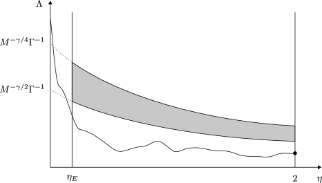
Figure 5.1: The $(\eta,\Lambda)$-plane for a fixed $E$. The shaded region is forbidden with high probability by Lemma 5.4. The initial estimate, given by Lemma 5.5, is marked with a black dot. The graph of $\Lambda=\Lambda(E+\mathrm{i}\eta)$ is continuous and lies beneath the shaded region. Note that this method does not control $\Lambda(E+i\eta)$ in the regime $\eta\leqslant\eta_{E}$.

Proof of Proposition 5.3.

Fix $D>10$. Lemma 5.4 implies that for each $z\in\bm{\mathrm{S}}$ we have

$$\mathbb{P}\Bigl{(}{M^{-\gamma/3}\Gamma(z)^{-1}\leqslant\Lambda(z)\leqslant M^{-\gamma/4}\Gamma(z)^{-1}}\Bigr{)}\;\leqslant\;N^{-D}$$ (5.21)

for $N\geqslant N_{0}$, where $N_{0}\equiv N_{0}(\gamma,D)$ does not depend on $z$.

Next, take a lattice $\Delta\subset\bm{\mathrm{S}}$ such that $\lvert\Delta\rvert\leqslant N^{10}$ and for each $z\in\bm{\mathrm{S}}$ there exists a $w\in\Delta$ such that $\lvert z-w\rvert\leqslant N^{-4}$. Then (5.21) combined with a union bounds gives

$$\mathbb{P}\Bigl{(}{\exists w\in\Delta\,\mathrel{\vbox{\hbox{.}\hbox{.}}}\,M^{-\gamma/3}\Gamma(w)^{-1}\leqslant\Lambda(w)\leqslant M^{-\gamma/4}\Gamma(w)^{-1}}\Bigr{)}\;\leqslant\;N^{-D+10}$$ (5.22)

for $N\geqslant N_{0}$. From the definitions of $\Lambda(z)$, $\Gamma(z)$, and $\bm{\mathrm{S}}$ (recall (4.5)), we immediately find that $\Lambda$ and $\Gamma$ are Lipschitz continuous on $\bm{\mathrm{S}}$, with Lipschitz constant at most $M^{2}$. Hence (5.22) implies

$$\mathbb{P}\Bigl{(}{\exists z\in\bm{\mathrm{S}}\,\mathrel{\vbox{\hbox{.}\hbox{.}}}\,2M^{-\gamma/3}\Gamma(z)^{-1}\leqslant\Lambda(z)\leqslant 2^{-1}M^{-\gamma/4}\Gamma(z)^{-1}}\Bigr{)}\;\leqslant\;N^{-D+10}$$

for $N\geqslant N_{0}$. We conclude that there is an event $\Xi$ satisfying $\mathbb{P}(\Xi)\geqslant 1-N^{-D+10}$ such that, for each $z\in\bm{\mathrm{S}}$, either $\bm{\mathrm{1}}(\Xi)\Lambda(z)\leqslant 2M^{-\gamma/3}\Gamma(z)^{-1}$ or $\bm{\mathrm{1}}(\Xi)\Lambda(z)\geqslant 2^{-1}M^{-\gamma/4}\Gamma(z)^{-1}$. Since $\Lambda$ is continuous and $\bm{\mathrm{S}}$ is by definition connected, we conclude that either

$$\forall z\in\bm{\mathrm{S}}\,\mathrel{\vbox{\hbox{.}\hbox{.}}}\,\bm{\mathrm{1}}(\Xi)\Lambda(z)\;\leqslant\;2M^{-\gamma/3}\Gamma(z)^{-1}$$ (5.23)

or

$$\forall z\in\bm{\mathrm{S}}\,\mathrel{\vbox{\hbox{.}\hbox{.}}}\,\bm{\mathrm{1}}(\Xi)\Lambda(z)\;\geqslant\;2^{-1}M^{-\gamma/4}\Gamma(z)^{-1}\,.$$ (5.24)

(Here the bounds (5.23) and (5.24) each hold surely, i.e. for every realization of $\Lambda(z)$.)

It remains to show that (5.24) is impossible. In order to do so, it suffices to show that there exists a $z\in\bm{\mathrm{S}}$ such that $\Lambda(z)<2^{-1}M^{-\gamma/4}\Gamma(z)^{-1}$ with probability greater than $1/2$. But this holds for any $z$ with $\operatorname{Im}z=2$, as follows from Lemma 5.5 and the bound $\Gamma\leqslant C\eta^{-1}$, which itself follows easily by a simple expansion of $(1-m^{2}S)^{-1}$ combined with the bounds $\lVert S\rVert_{\ell^{\infty}\to\ell^{\infty}}\leqslant 1$ and (4.2). This concludes the proof. ∎

5.4.  Iteration step and conclusion of the proof of Theorem 5.1

In the following a key role will be played by deterministic control parameters $\Psi$ satisfying

$$cM^{-1/2}\;\leqslant\;\Psi\;\leqslant\;M^{-\gamma/3}\Gamma^{-1}\,.$$ (5.25)

(Using the definition of $\bm{\mathrm{S}}$ and (4.4) it is not hard to check that the upper bound in (5.25) is always larger than the lower bound.) Suppose that $\Lambda\prec\Psi$ in $\bm{\mathrm{S}}$ for some deterministic parameter $\Psi$ satisfying (5.25). For example, by Proposition 5.3 we may choose $\Psi=M^{-\gamma/3}\Gamma^{-1}$.

We now improve the estimate $\Lambda\prec\Psi$ iteratively. The iteration step is the content of the following proposition.

Proposition 5.6.

Let $\Psi$ be a control parameter satisfying (5.25) and fix $\varepsilon\in(0,\gamma/3)$. Then

$$\Lambda\;\prec\;\Psi\qquad\Longrightarrow\qquad\Lambda\;\prec\;F(\Psi)\,,$$ (5.26)

where we defined

$$F(\Psi)\;\mathrel{\vbox{\hbox{.}\hbox{.}}}=\;M^{-\varepsilon}\Psi+\sqrt{\frac{\operatorname{Im}m}{M\eta}}+\frac{M^{\varepsilon}}{M\eta}\,.$$

For the proof of Proposition 5.6 we need the following averaging result, which is a simple corollary of Theorem 4.6.

Lemma 5.7.

Suppose that $\Lambda\prec\Psi$ for some deterministic control parameter $\Psi$ satisfying (4.8). Then $[\Upsilon]=O_{\prec}(\Psi^{2})$ (recall the definition of the average $[\cdot]$ from (4.10)).

Proof.

The claim easily follows from Schur’s complement formula (5.6) written in the form

$$\Upsilon_{i}\;=\;A_{i}+Q_{i}\frac{1}{G_{ii}}\,.$$

We may therefore estimate $[\Upsilon]$ using the trivial bound $\lvert A_{i}\rvert\prec\Psi^{2}$ as well as the fluctuation averaging bound from the first estimate of (4.11) with $t_{ik}=1/N$. ∎

Proof of Proposition 5.6.

Suppose that $\Lambda\prec\Psi$ for some deterministic control parameter $\Psi$ satisfying (5.25). We invoke Lemma 5.2 with $\phi=1$ (recall the bound (4.5)) to get

$$\Lambda_{o}+\lvert Z_{i}\rvert+\lvert\Upsilon_{i}\rvert\;\prec\;\sqrt{\frac{\operatorname{Im}m+\Lambda}{M\eta}}\;\prec\;\sqrt{\frac{\operatorname{Im}m+\Psi}{M\eta}}\,.$$ (5.27)

Next, we estimate $\Lambda_{d}$. Define the $z$-dependent indicator function

$$\psi\;\mathrel{\vbox{\hbox{.}\hbox{.}}}=\;\bm{\mathrm{1}}(\Lambda\leqslant M^{-\gamma/4})\,.$$

By (5.25), (4.5), and the assumption $\Lambda\prec\Psi$, we have $1-\psi\prec 0$. On the event $\{\psi=1\}$, we expand the right-hand side of (5.9) to get the bound

$$\psi\lvert v_{i}\rvert\;\leqslant\;C\psi\biggl{\lvert}\sum_{k}s_{ik}v_{k}-\Upsilon_{i}\biggr{\rvert}+C\psi\Lambda^{2}\,.$$

Using the fluctuation averaging estimate (4.12) as well as (5.27), we find

$$\psi\lvert v_{i}\rvert\;\prec\;\Gamma\Psi^{2}+\sqrt{\frac{\operatorname{Im}m+\Psi}{M\eta}}\,,$$ (5.28)

where we again used the lower bound from (4.5). Using $1-\psi\prec 0$ we conclude

$$\Lambda_{d}\;\prec\;\Gamma\Psi^{2}+\sqrt{\frac{\operatorname{Im}m+\Psi}{M\eta}}\,,$$ (5.29)

which, combined with (5.27), yields

$$\Lambda\;\prec\;\Gamma\Psi^{2}+\sqrt{\frac{\operatorname{Im}m+\Psi}{M\eta}}\,.$$ (5.30)

Using Young’s inequality and the assumption $\Psi\leqslant M^{-\gamma/3}\Gamma^{-1}$ we conclude the proof. ∎

For the remainder of the proof of Theorem 5.1 we work on the spectral domain $\bm{\mathrm{S}}$. We claim that if $\Psi$ satisfies (5.25) then so does $F(\Psi)$. The lower bound $F(\Psi)\geqslant cM^{-1/2}$ is a consequence of the estimate $\operatorname{Im}m/\eta\geqslant c$, which follows from (4.4). The upper bound $M^{-\gamma/3-\varepsilon}\Gamma^{-1}$ on the first term of $F(\Psi)$ is trivial by assumption on $\Psi$. Moreover, the second term of $F(\Psi)$ satisfies $\sqrt{\operatorname{Im}m/(M\eta)}\leqslant M^{-\gamma}\Gamma^{-2}\leqslant CM^{-\gamma}\Gamma^{-1}\leqslant M^{-\gamma/3-\varepsilon}\Gamma^{-1}$ by definition of $\bm{\mathrm{S}}$ and the lower bound (4.5). Similarly, the last term of $F(\Psi)$ satisfies $M^{\varepsilon}/(M\eta)\leqslant CM^{\varepsilon-\gamma}\Gamma^{-1}\leqslant M^{-\gamma/3-\varepsilon}\Gamma^{-1}$ by definition of $\bm{\mathrm{S}}$.

We may therefore iterate (5.26). This yields a bound on $\Lambda$ that is essentially the fixed point of the map $\Psi\mapsto F(\Psi)$, which is $\Pi$ (up to the factor $M^{\varepsilon}$). More precisely, the iteration is started with $\Psi_{0}\mathrel{\vbox{\hbox{.}\hbox{.}}}=M^{-\gamma/3}\Gamma^{-1}$; the initial hypothesis $\Lambda\prec\Psi_{0}$ is provided by the rough bound from Proposition 5.3. For $k\geqslant 1$ we set $\Psi_{k+1}\mathrel{\vbox{\hbox{.}\hbox{.}}}=F(\Psi_{k})$. Hence from (5.26) we conclude that $\Lambda\prec\Psi_{k}$ for all $k$. Choosing $k\mathrel{\vbox{\hbox{.}\hbox{.}}}=\lceil{\varepsilon^{-1}}\rceil$ yields

$$\Lambda\;\prec\;\sqrt{\frac{\operatorname{Im}m}{M\eta}}+\frac{M^{\varepsilon}}{M\eta}\,.$$

Since $\varepsilon$ was arbitrary, we have proved that

$$\Lambda\;\prec\;\Pi\,,$$ (5.31)

which is (5.3).

What remains is to prove (5.4), i.e. to estimate $\Theta$. We expand (5.9) on $\{\psi=1\}$ to get

$$\psi m^{2}\biggl{(}{-\sum_{k}s_{ik}v_{k}+\Upsilon_{i}}\biggr{)}\;=\;-\psi v_{i}+O(\psi\Lambda^{2})\,.$$ (5.32)

Averaging in (5.32) yields

$$\psi m^{2}\bigl{(}{-[v]+[\Upsilon]}\bigr{)}\;=\;-\psi[v]+O(\psi\Lambda^{2})\,.$$

By (5.31) and (5.27) with $\Psi=\Pi$, we have $\Lambda+\lvert\Upsilon_{i}\rvert\prec\Pi$. Moreover, by Lemma 5.7 we have $\lvert[\Upsilon]\rvert\prec\Pi^{2}$. Thus we get

$$\psi[v]\;=\;m^{2}\psi[v]+O_{\prec}(\Pi^{2})\,.$$

Since $1-\psi\prec 0$, we conclude that $[v]=m^{2}[v]+O_{\prec}(\Pi^{2})$. Therefore

$$\lvert[v]\rvert\;\prec\;\frac{\Pi^{2}}{\lvert 1-m^{2}\rvert}\;\leqslant\;\biggl{(}{\frac{\operatorname{Im}m}{\lvert 1-m^{2}\rvert}+\frac{1}{\lvert 1-m^{2}\rvert M\eta}}\biggr{)}\frac{2}{M\eta}\;\leqslant\;\biggl{(}{C+\frac{\Gamma}{M\eta}}\biggr{)}\frac{2}{M\eta}\;\leqslant\;\frac{C}{M\eta}\,.$$

Here in the third step we used (4.3), (4.4), and the bound $\Gamma\geqslant\lvert 1-m^{2}\rvert^{-1}$ which follows from the definition of $\Gamma$ by applying the matrix $(1-m^{2}S)^{-1}$ to the vector $\bm{\mathrm{e}}=N^{-1/2}(1,1,\dots,1)^{*}$. The last step follows from the definition of $\bm{\mathrm{S}}$. Since $\Theta=\lvert[v]\rvert$, this concludes the proof of (5.4), and hence of Theorem 5.1.

6 Proof of Theorem 2.3

The key novelty in this proof is that we solve the self-consistent equation (5.9) separately on the subspace of constants (the span of the vector $\bm{\mathrm{e}}$) and on its orthogonal complement $\bm{\mathrm{e}}^{\perp}$. On the space of constant vectors, it becomes a scalar equation for the average $[v]$, which can be expanded up to second order. Near the spectral edges $\pm 2$, the resulting quadratic self-consistent scalar equation (given in (6.2) below) is more effective than its linearized version. On the space orthogonal to the constants, we still solve a self-consistent vector equation, but the stability will now be quantified using $\widetilde{\Gamma}$ instead of the larger quantity $\Gamma$.

Accordingly, the main control parameter in this proof is $\Theta=\lvert[v]\rvert$, and the key iterative scheme (Lemma 6.7 below) is formulated in terms of $\Theta$. However, many intermediate estimates still involve $\Lambda$. In particular, the self-consistent equation (5.9) is effective only in the regime where $v_{i}$ is already small. Hence we need two preparatory steps. In Section 6.1 we will prove an apriori bound on $\Lambda$, essentially showing that $\Lambda\ll 1$. This proof itself is a continuity argument (see Figure 6.1 for a graphical illustration) similar to the proof of Proposition 5.3; now, however, we have to follow $\Lambda$ and $\Theta$ in tandem. The main reason why $\Theta$ is already involved in this part is that we work in larger spectral domain $\widetilde{\bm{\mathrm{S}}}$ defined using $\widetilde{\Gamma}$. Thus, already in this preparatory step, the self-consistent equation has to be solved separately on the subspace of constants and its orthogonal complement.

In Section 6.2, we control $\Lambda$ in terms of $\Theta$, which allows us to obtain a self-consistent equation involving only $\Theta$. In this step we use the Fluctuation Averaging Theorem to obtain a quadratic estimate which, very roughly, states that $\Lambda\lesssim\Theta+\Lambda^{2}$ (see (6.20) below for the precise statement). This implies $\Lambda\lesssim\Theta$ in the regime $\Lambda\ll 1$.

Finally, in Section 6.3, we solve the quadratic iteration for $\Theta$. Since the corresponding quadratic equation has a dichotomy and for large $\eta=\operatorname{Im}z$ we know that $\Theta$ is small by direct expansion, a continuity argument similar to the proof of Proposition 5.3 will complete the proof.

6.1.  A rough bound on $\Lambda$

In this section we prove the following apriori bounds on both control parameters, $\Lambda$ and $\Theta$.

Proposition 6.1.

In $\widetilde{\bm{\mathrm{S}}}$ we have the bounds

$$\Lambda\;\prec\;M^{-\gamma/4}\widetilde{\Gamma}^{-1}\,,\qquad\Theta\;\prec\;(M\eta)^{-1/3}\,.$$

Before embarking on the proof of Proposition 6.1, we state some preparatory lemmas. First, we derive the key equation for $[v]=N^{-1}\sum_{i}v_{i}$, the average of $v_{i}$.

Lemma 6.2.

Define the $z$-dependent indicator function

$$\phi\;\mathrel{\vbox{\hbox{.}\hbox{.}}}=\;\bm{\mathrm{1}}(\Lambda\leqslant M^{-\gamma/4}\widetilde{\Gamma}^{-1})$$ (6.1)

and the random control parameter

$$q(\Theta)\;\mathrel{\vbox{\hbox{.}\hbox{.}}}=\;\sqrt{\frac{\operatorname{Im}m+\Theta}{M\eta}}+\frac{\widetilde{\Gamma}}{M\eta}\,.$$

Then we have

$$\phi\Bigl{(}{(1-m^{2})[v]-m^{-1}[v]^{2}}\Bigr{)}\;=\;\phi\,O_{\prec}\bigl{(}{q(\Theta)+M^{-\gamma/4}\Theta^{2}}\bigr{)}$$ (6.2)

and

$$\phi\Lambda\;\prec\;\Theta+\widetilde{\Gamma}\,q(\Theta)\,.$$ (6.3)

Proof.

For the whole proof we work on the event $\{\phi=1\}$, i.e. every quantity is multiplied by $\phi$. We consistently drop these factors $\phi$ from our notation in order to avoid cluttered expressions. In particular, $\Lambda\leqslant CM^{-\gamma/4}$ throughout the proof.

We begin by estimating $\Lambda_{o}$ and $\Lambda_{d}$ in terms of $\Theta$. Recalling (4.5), we find that $\phi$ satisfies the hypotheses of Lemma 5.2, from which we get

$$\Lambda_{o}+\lvert\Upsilon_{i}\rvert\;\prec\;r(\Lambda)\,,\qquad r(\Lambda)\;\mathrel{\vbox{\hbox{.}\hbox{.}}}=\;\sqrt{\frac{\operatorname{Im}m+\Lambda}{M\eta}}\,.$$ (6.4)

In order to estimate $\Lambda_{d}$, we expand the self-consistent equation (5.9) (on the event $\{\phi=1\}$) to get

$$v_{i}-m^{2}\sum_{k}s_{ik}v_{k}\;=\;O_{\prec}\bigl{(}{\Lambda^{2}+r(\Lambda)}\bigr{)}\,;$$ (6.5)

here we used the bound (6.4) on $|\Upsilon_{i}|$. Next, we subtract the average $N^{-1}\sum_{i}$ from each side to get

$$(v_{i}-[v])-m^{2}\sum_{k}s_{ik}(v_{k}-[v])\;=\;O_{\prec}\bigl{(}{\Lambda^{2}+r(\Lambda)}\bigr{)}\,.$$

Note that the average of the left-hand side vanishes, so that the average of the right-hand side also vanishes. Hence the right-hand side is perpendicular to $\bm{\mathrm{e}}$. Inverting the operator $1-m^{2}S$ on the subspace $\bm{\mathrm{e}}^{\perp}$ therefore yields

$$\bigl{\lvert}v_{i}-[v]\bigr{\rvert}\;\prec\;\widetilde{\Gamma}\bigl{(}{\Lambda^{2}+r(\Lambda)}\bigr{)}\,.$$ (6.6)

Combining with the bound $\Lambda_{o}\prec r(\Lambda)$ from (6.4), we therefore get

$$\Lambda\;\prec\;\Theta+\widetilde{\Gamma}\Lambda^{2}+\widetilde{\Gamma}r(\Lambda)\,.$$ (6.7)

By definition of $\phi$ we have $\widetilde{\Gamma}\Lambda^{2}\leqslant M^{-\gamma/4}\Lambda$, so that by Lemma 4.4 (iii) the second term on the right-hand side of (6.7) may be absorbed into the left-hand side:

$$\Lambda\;\prec\;\Theta+\widetilde{\Gamma}r(\Lambda)\,.$$ (6.8)

Now we claim that

$$r(\Lambda)\;\prec\;q(\Theta)\,.$$ (6.9)

If (6.9) is proved, clearly (6.3) follows from (6.8). In order to prove (6.9), we use (6.8) and the Cauchy-Schwarz inequality to get

$$r(\Lambda)\;\leqslant\;\sqrt{\frac{\operatorname{Im}m}{M\eta}}+\sqrt{\frac{\Lambda}{M\eta}}\;\prec\;\sqrt{\frac{\operatorname{Im}m}{M\eta}}+\sqrt{\frac{\Theta}{M\eta}}+\sqrt{\frac{\widetilde{\Gamma}\,r(\Lambda)}{M\eta}}\;\leqslant\;\sqrt{\frac{\operatorname{Im}m}{M\eta}}+\sqrt{\frac{\Theta}{M\eta}}+M^{-\varepsilon}r(\Lambda)+M^{\varepsilon}\frac{\widetilde{\Gamma}}{M\eta}$$

for any $\varepsilon>0$. We conclude that

$$r(\Lambda)\;\prec\;\sqrt{\frac{\operatorname{Im}m}{M\eta}}+\sqrt{\frac{\Theta}{M\eta}}+M^{\varepsilon}\frac{\widetilde{\Gamma}}{M\eta}\,.$$

Since $\varepsilon>0$ was arbitrary, (6.9) follows.

Next, we estimate $\Theta$. We expand (5.9) to second order:

$$-\sum_{k}s_{ik}v_{k}+\Upsilon_{i}\;=\;-\frac{1}{m^{2}}v_{i}+\frac{1}{m^{3}}v_{i}^{2}+O(\Lambda^{3})\,.$$ (6.10)

In order to take the average and get a closed equation for $[v]$, we write, using (6.6),

$$v_{i}^{2}\;=\;\bigl{(}{[v]+v_{i}-[v]}\bigr{)}^{2}\;=\;[v]^{2}+2[v](v_{i}-[v])+O_{\prec}\Bigl{(}{\widetilde{\Gamma}^{2}\bigl{(}{\Lambda^{2}+r(\Lambda)}\bigr{)}^{2}}\Bigr{)}\,.$$

Plugging this back into (6.10) and taking the average over $i$ gives

$$-m^{2}[v]+m^{2}[\Upsilon]\;=\;-[v]+m^{-1}[v]^{2}+O_{\prec}\Bigl{(}{\Lambda^{3}+\widetilde{\Gamma}^{2}\Lambda^{4}+\widetilde{\Gamma}^{2}r(\Lambda)^{2}}\Bigr{)}\,.$$

Estimating $[\Upsilon]$ by $\max\lvert\Upsilon_{i}\rvert\prec r(\Lambda)$ (recall (6.4)) yields

$$(1-m^{2})[v]-m^{-1}[v]^{2}\;=\;O_{\prec}\Bigl{(}{r(\Lambda)+\Lambda^{3}+\widetilde{\Gamma}^{2}\Lambda^{4}+\widetilde{\Gamma}^{2}r(\Lambda)^{2}}\Bigr{)}\,.$$

By definitions of $\widetilde{\bm{\mathrm{S}}}$ and $\phi$, we have $\widetilde{\Gamma}^{2}r(\Lambda)\leqslant 1$. Therefore we may absorb the last error term into the first. For the second and third error terms we use (6.8) to get

$$(1-m^{2})[v]-m^{-1}[v]^{2}\;=\;O_{\prec}\Bigl{(}{r(\Lambda)+\Theta^{3}+\widetilde{\Gamma}^{3}r(\Lambda)^{3}+\widetilde{\Gamma}^{2}\Theta^{4}+\widetilde{\Gamma}^{6}r(\Lambda)^{4}}\Bigr{)}\,.$$

In order to conclude the proof of (6.2), we observe that, by the estimates $\Theta\leqslant\Lambda\leqslant CM^{-\gamma/4}$, $\widetilde{\Gamma}^{2}r(\Lambda)\leqslant 1$, and $\Lambda\leqslant M^{-\gamma/4}\widetilde{\Gamma}^{-1}$, we have

$$\Theta^{3}\;\leqslant\;CM^{-\gamma/4}\Theta^{2}\,,\qquad\widetilde{\Gamma}^{3}r(\Lambda)^{3}\;\leqslant\;r(\Lambda)\,,\qquad\widetilde{\Gamma}^{2}\Theta^{4}\;\leqslant\;\widetilde{\Gamma}^{2}\Lambda^{2}\Theta^{2}\;\leqslant\;M^{-\gamma/2}\Theta^{2}\,,\qquad\widetilde{\Gamma}^{6}r(\Lambda)^{4}\;\leqslant\;r(\Lambda)\,.$$

Putting everything together, we have

$$(1-m^{2})[v]-m^{-1}[v]^{2}\;=\;O_{\prec}\bigl{(}{r(\Lambda)+M^{-\gamma/4}\Theta^{2}}\bigr{)}\,.$$

Hence (6.2) follows from (6.9). ∎

Next, we establish a bound analogous to Lemma 5.4, establishing gaps in the ranges of $\Lambda$ and $\Theta$. To that end, we need to partition $\widetilde{\bm{\mathrm{S}}}$ in two. For the following we fix $\varepsilon\in(0,\gamma/12)$ and partition $\widetilde{\bm{\mathrm{S}}}=\widetilde{\bm{\mathrm{S}}}_{>}\cup\widetilde{\bm{\mathrm{S}}}_{\leqslant}$, where

$$\widetilde{\bm{\mathrm{S}}}_{>}\;\mathrel{\vbox{\hbox{.}\hbox{.}}}=\;\bigl{\{}{z\in\widetilde{\bm{\mathrm{S}}}\mathrel{\vbox{\hbox{.}\hbox{.}}}\sqrt{\kappa+\eta}>M^{\varepsilon}(M\eta)^{-1/3}}\bigr{\}}\,,\qquad\widetilde{\bm{\mathrm{S}}}_{\leqslant}\;\mathrel{\vbox{\hbox{.}\hbox{.}}}=\;\bigl{\{}{z\in\widetilde{\bm{\mathrm{S}}}\mathrel{\vbox{\hbox{.}\hbox{.}}}\sqrt{\kappa+\eta}\leqslant M^{\varepsilon}(M\eta)^{-1/3}}\bigr{\}}.$$

The bound relies on (6.2), whereby one of the two terms on the left-hand side of (6.2) is estimated in terms of all the other terms, which are regarded as an error. In $\widetilde{\bm{\mathrm{S}}}_{>}$ we shall estimate the first term on the left-hand side of (6.2), and in $\widetilde{\bm{\mathrm{S}}}_{\leqslant}$ the second. Figure 6.1 summarizes the estimates on $\Theta$ of Lemma 6.3 and 6.4.

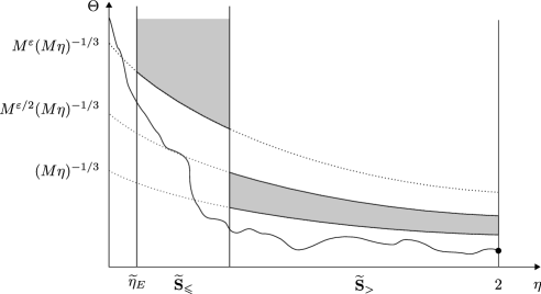
Figure 6.1: The $(\eta,\Theta)$-plane for a fixed $E$ near the edge (i.e. with small $\kappa$). The shaded regions are forbidden with high probability by Lemmas 6.3 and 6.4. The initial estimate, given by Lemma 5.5, is marked with a black dot. The graph of $\Theta=\Theta(E+\mathrm{i}\eta)$ is continuous, and hence lies beneath the shaded regions.

We begin with the domain $\widetilde{\bm{\mathrm{S}}}_{>}$. In this domain, the following lemma roughly says that if $\Theta\leqslant M^{\varepsilon/2}(M\eta)^{-1/3}$ and $\Lambda\leqslant M^{-\gamma/4}\widetilde{\Gamma}^{-1}$ then we get the improved bounds $\Theta\prec(M\eta)^{-1/3}$, $\Lambda\prec M^{-\gamma/3}\widetilde{\Gamma}^{-1}$, i.e. we gain a small power of $M$. These improvements will be fed into the continuity argument as before.

Lemma 6.3.

Let $\varepsilon\in(0,\gamma/12)$. Define the $z$-dependent indicator function

$$\chi\;\mathrel{\vbox{\hbox{.}\hbox{.}}}=\;\bm{\mathrm{1}}\Bigl{(}{\Theta\leqslant M^{\varepsilon/2}(M\eta)^{-1/3}}\Bigr{)}$$

and recall the indicator function $\phi$ from (6.1). In $\widetilde{\bm{\mathrm{S}}}_{>}$ we have the bounds

$$\phi\chi\,\Theta\;\prec\;(M\eta)^{-1/3}\,,\qquad\phi\chi\,\Lambda\;\prec\;M^{-\gamma/3}\widetilde{\Gamma}^{-1}\,.$$ (6.11)

Proof.

From the definition of $\widetilde{\bm{\mathrm{S}}}_{>}$ and (4.3) we get

$$\phi\chi\,\lvert[v]\rvert\;=\;\phi\chi\,\Theta\;\leqslant\;M^{\varepsilon/2}(M\eta)^{-1/3}\;\leqslant\;M^{-\varepsilon/2}\sqrt{\kappa+\eta}\;\leqslant\;CM^{-\varepsilon/2}\lvert 1-m^{2}\rvert\,.$$

Therefore, on the event $\{\phi\chi=1\}$, in (6.2) we may absorb the second term on the left-hand side and the second term on the right-hand side into the first term on the left-hand side:

$$\phi\chi\,(1-m^{2})[v]\;=\;\phi O_{\prec}\bigl{(}{q(\Theta)}\bigr{)}\,.$$

Recalling $|1-m^{2}|\asymp\sqrt{\kappa+\eta}$ (see (4.3)), $\operatorname{Im}m\leqslant C\sqrt{\kappa+\eta}$ (see (4.4)), (6.9), $\lvert[v]\rvert=\Theta$, and the definition of $\widetilde{\bm{\mathrm{S}}}_{>}$, we get

$$\phi\chi\,\Theta \;\prec\;\phi\chi\,(\kappa+\eta)^{-1/2}\Biggl{(}{\sqrt{\frac{\operatorname{Im}m}{M\eta}}+\sqrt{\frac{\Theta}{M\eta}}+\frac{\widetilde{\Gamma}}{M\eta}}\Biggr{)}$$

$$\;\leqslant\;(\kappa+\eta)^{-1/4}(M\eta)^{-1/2}+(\kappa+\eta)^{-1/2}M^{\varepsilon/2}(M\eta)^{-2/3}+(\kappa+\eta)^{-1/2}\widetilde{\Gamma}(M\eta)^{-1}$$

$$\;\leqslant\;(M\eta)^{-1/3}\,.$$

What remains is to estimate $\Lambda$. From (6.3), the bound $\widetilde{\Gamma}^{2}\sqrt{\operatorname{Im}m(M\eta)^{-1}}\leqslant M^{-\gamma}$ from the definition of $\widetilde{\bm{\mathrm{S}}}$, and the estimate $\phi\widetilde{\Gamma}\Theta\leqslant\phi\widetilde{\Gamma}\Lambda\leqslant 1$ we get

$$\phi\chi\,\Lambda \;\prec\;\phi\chi\,\Theta+M^{-\gamma}\widetilde{\Gamma}^{-1}+\widetilde{\Gamma}\sqrt{\widetilde{\Gamma}^{-1}(M\eta)^{-1}}+\widetilde{\Gamma}^{2}(M\eta)^{-1}$$

$$\;\prec\;(M\eta)^{-1/3}+M^{-\gamma/2}\widetilde{\Gamma}^{-1}+M^{-\gamma}\widetilde{\Gamma}^{-1}$$

$$\;\leqslant\;2M^{-\gamma/3}\widetilde{\Gamma}^{-1}\,.$$

This concludes the proof. ∎

Next, we establish a gap in the range of $\Lambda$, in the domain $\widetilde{\bm{\mathrm{S}}}_{\leqslant}$. To that end, we improve the estimate on $\Lambda$ from $\Lambda\leqslant M^{-\gamma/4}\widetilde{\Gamma}^{-1}$ to $\Lambda\prec M^{\varepsilon-\gamma/3}\widetilde{\Gamma}^{-1}$ as before. In this regime there is no need for a gap in $\Theta$, i.e. the continuity argument will be performed on the value of $\Lambda$ only.

Lemma 6.4.

In $\widetilde{\bm{\mathrm{S}}}_{\leqslant}$ we have the bounds

$$\phi\Theta\;\prec\;M^{\varepsilon}(M\eta)^{-1/3}\,,\qquad\phi\Lambda\;\prec\;M^{\varepsilon-\gamma/3}\widetilde{\Gamma}^{-1}\,.$$ (6.12)

Proof.

We write (6.2) as

$$\phi[v](1-m^{2}-m^{-1}[v])\;=\;\phi\,O_{\prec}\bigl{(}{q(\Theta)+M^{-\gamma/4}\Theta^{2}}\bigr{)}.$$

Solving this quadratic relation for $[v]$, we get

$$\phi\Theta\;\prec\;\lvert 1-m^{2}\rvert+\phi\sqrt{q(\Theta)+M^{-\gamma/4}\Theta^{2}}\,.$$ (6.13)

Using (4.4), the bound $\widetilde{\Gamma}\leqslant M^{-\gamma/3}(M\eta)^{1/3}\leqslant(M\eta)^{1/3}$ from the definition of $\widetilde{\bm{\mathrm{S}}}$, and Young’s inequality, we estimate

$$\sqrt{q(\Theta)+M^{-\gamma/4}\Theta^{2}} \;\leqslant\;(\operatorname{Im}m)^{1/4}(M\eta)^{-1/4}+\Theta^{1/4}(M\eta)^{-1/4}+\widetilde{\Gamma}^{\,1/2}(M\eta)^{-1/2}+M^{-\gamma/8}\Theta$$

$$\;\leqslant\;C\sqrt{\kappa+\eta}+CM^{\varepsilon}(M\eta)^{-1/3}+CM^{-\varepsilon}\Theta\,.$$

Plugging this bound into (6.13), together with (4.3) and the definition of $\widetilde{\bm{\mathrm{S}}}_{\leqslant}$, we find

$$\phi\Theta\;\prec\;\sqrt{\kappa+\eta}+M^{\varepsilon}(M\eta)^{-1/3}\;\leqslant\;2M^{\varepsilon}(M\eta)^{-1/3}\,.$$

This proves the first bound of (6.12).

What remains is the estimate of $\Lambda$. From (6.3) and the bounds $\widetilde{\Gamma}\leqslant M^{-\gamma/3}(M\eta)^{1/3}$ and $\widetilde{\Gamma}^{2}\sqrt{\operatorname{Im}m(M\eta)^{-1}}\leqslant M^{-\gamma}$ from the definition of $\widetilde{\bm{\mathrm{S}}}$, we get

$$\phi\Lambda \;\prec\;\phi\Theta+M^{-\gamma}\widetilde{\Gamma}^{-1}+\widetilde{\Gamma}\sqrt{\widetilde{\Gamma}^{-1}(M\eta)^{-1}}+\widetilde{\Gamma}^{2}(M\eta)^{-1}$$

$$\;\prec\;M^{\varepsilon}(M\eta)^{-1/3}+M^{-\gamma/2}\widetilde{\Gamma}^{-1}+M^{-\gamma}\widetilde{\Gamma}^{-1}$$

$$\;\leqslant\;2M^{\varepsilon-\gamma/3}\widetilde{\Gamma}^{-1}\,.$$

This concludes the proof. ∎

We now have all of the ingredients to complete the proof of Proposition 6.1.

Proof of Proposition 6.1.

The proof is a continuity argument similar to the proof of Proposition 5.3. In a first step, we prove that

$$\Lambda\;\prec\;M^{-\gamma/3}\widetilde{\Gamma}^{-1}\,,\qquad\Theta\;\prec\;(M\eta)^{-1/3}\,.$$ (6.14)

in $\widetilde{\bm{\mathrm{S}}}_{>}$. The continuity argument is almost identical to that following (5.21); the only difference is that we keep track of the two parameters $\Lambda$ and $\Theta$. The required gaps in the ranges of $\Lambda$ and $\Theta$ are provided by (6.11), and the argument is closed using the large-$\eta$ estimate from Lemma 5.5, which yields $\Theta\leqslant\Lambda\prec M^{-1/2}$ for $\eta=2$.

In a second step, we prove that

$$\Lambda\;\prec\;M^{\varepsilon-\gamma/4}\widetilde{\Gamma}^{-1}\,,\qquad\Theta\;\prec\;M^{\varepsilon}(M\eta)^{-1/3}$$

in $\widetilde{\bm{\mathrm{S}}}_{\leqslant}$. This is again a continuity argument almost identical to that following (5.21). Now we establish a gap only in the range of $\Lambda$. The gap is provided by (6.12) (recall that by definition of $\varepsilon$ we have $\varepsilon-\gamma/3<-\gamma/4$), and the argument is closed using the bound (6.14) at the boundary of the domains $\widetilde{\bm{\mathrm{S}}}_{>}$ and $\widetilde{\bm{\mathrm{S}}}_{\leqslant}$.

The claim now follows since we may choose $\varepsilon\in(0,\gamma/12)$ to be arbitrarily small. This concludes the proof of Proposition 6.1. ∎

6.2.  An improved bound on $\Lambda$ in terms of $\Theta$

In (6.3) we already estimated $\Lambda$ in terms of $\Theta$; the goal of this section is to improve this bound by removing the factor $\widetilde{\Gamma}$ from that estimate. We do this using the Fluctuation Averaging Theorem, but we stress that the removal of a factor $\widetilde{\Gamma}$ is not the main rationale for using the fluctuation averaging mechanism. Its fundamental use will take place in Lemma 6.6 below. A technical consequence of invoking fluctuation averaging is that we have to use deterministic control parameters instead of random ones. Thus, we introduce a deterministic control parameter $\Phi$ that captures the size of the random control parameter $\Theta$ through the relation $\Theta\prec\Phi$. Throughout the following we shall make use of the control parameter

$$p(\Phi)\;\mathrel{\vbox{\hbox{.}\hbox{.}}}=\;\sqrt{\frac{\operatorname{Im}m+\Phi}{M\eta}}+\frac{1}{M\eta}\,,$$

which differs from $q(\Phi)$ only by a factor $\widetilde{\Gamma}$ in the second term.

Lemma 6.5.

Suppose that $\Lambda\prec\Psi$ and $\Theta\prec\Phi$ in $\widetilde{\bm{\mathrm{S}}}$ for some deterministic control parameters $\Psi$ and $\Phi$ satisfying

$$cM^{-1/2}\;\leqslant\;\Psi\;\leqslant\;CM^{-\gamma/4}\widetilde{\Gamma}^{-1}\,,\qquad\Phi\;\leqslant\;CM^{-\gamma/4}\widetilde{\Gamma}^{-1}\,.$$ (6.15)

Then

$$\Lambda_{o}+\lvert Z_{i}\rvert\;\prec\;p(\Phi)\,,\qquad\Lambda\;\prec\;p(\Phi)+\Phi\,.$$ (6.16)

We remark that, by Proposition 6.1, the choice $\Psi=M^{-\gamma/4}\widetilde{\Gamma}^{-1}$ and $\Phi=(M\eta)^{-1/3}\leqslant M^{-\gamma/4}\widetilde{\Gamma}^{-1}$ satisfies the assumptions of Lemma 6.5.

Proof of Lemma 6.5.

Choosing $\phi=1$ in Lemma 5.2 and recalling (4.5), we get

$$\Lambda_{o}+\lvert\Upsilon_{i}\rvert\;\prec\;r(\Psi)\,,\qquad r(\Psi)\;\mathrel{\vbox{\hbox{.}\hbox{.}}}=\;\sqrt{\frac{\operatorname{Im}m+\Psi}{M\eta}}\,.$$ (6.17)

In order to estimate $\Lambda_{d}$, as in (5.32), we expand (5.9) to get

$$-\sum_{k}s_{ik}v_{k}+\Upsilon_{i}\;=\;-m^{-2}v_{i}+O_{\prec}(\Psi^{2})\,.$$ (6.18)

As in the proof of (5.32) and (6.5), the expansion of (5.9) is only possible on the event $\{\Lambda\leqslant M^{-\delta}\}$ for some $\delta>0$. By $\Lambda\prec\Psi$ and (6.15), the indicator function of this event is $1+O_{\prec}(0)$; the contribution $O_{\prec}(0)$ of the complementary event can be absorbed in the error term $O_{\prec}(\Psi^{2})$.

Subtracting the average $N^{-1}\sum_{i}$ from both sides of (6.18) and estimating $m^{2}$ by a constant (see (4.2)) yields

$$\bigl{\lvert}v_{i}-[v]\bigr{\rvert}\;\leqslant\;C\biggl{\lvert}\sum_{k}s_{ik}\bigl{(}{v_{k}-[v]}\bigr{)}-\bigl{(}{\Upsilon_{i}-[\Upsilon]}\bigr{)}\biggr{\rvert}+O_{\prec}(\Psi^{2})\;\prec\;\widetilde{\Gamma}\Psi^{2}+r(\Psi)\,,$$ (6.19)

where in the last step we used the fluctuation averaging estimate (4.14) and $\lvert\Upsilon_{i}\rvert\prec r(\Psi)$ from (6.17). Together with $\lvert[v]\rvert=\Theta\prec\Phi$ , this gives the estimate $\Lambda_{d}\prec\Gamma\Psi^{2}+\Phi+r(\Psi)$. Combining it with the bound (6.17), we conclude that

$$\Lambda\prec\widetilde{\Gamma}\Psi^{2}+\Phi+r(\Psi).$$ (6.20)

Now fix $\varepsilon\in(0,\gamma/4)$. Using the assumption $\widetilde{\Gamma}\Psi\leqslant CM^{-\gamma/4}\leqslant M^{-\varepsilon}$, we conclude: if $\Psi$ and $\Phi$ satisfy (6.15) then

$$\Lambda\;\prec\;\Psi\qquad\Longrightarrow\qquad\Lambda\;\prec\;F(\Psi,\Phi)\,,$$ (6.21)

where we defined

$$F(\Psi,\Phi)\;\mathrel{\vbox{\hbox{.}\hbox{.}}}=\;M^{-\varepsilon}\Psi+\Phi+\sqrt{\frac{\operatorname{Im}m}{M\eta}}+\frac{M^{\varepsilon}}{M\eta}\,,$$

which plays a role similar to $F(\Psi)$ in Proposition 5.6. (Here we estimated $\sqrt{\Psi(M\eta)^{-1}}$ in $r(\Psi)$ by $M^{-\varepsilon}\Psi+M^{\varepsilon}(M\eta)^{-1}$.) From (4.4) and the definition of $\widetilde{\bm{\mathrm{S}}}$ it easily follows that if $(\Psi,\Phi)$ satisfy (6.15) then so do $(F(\Psi,\Phi),\Phi)$. Therefore iterating (6.21) $\lceil{\varepsilon^{-1}}\rceil$ times and using the fact that $\varepsilon\in(0,\gamma/4)$ was arbitrary yields

$$\Lambda\;\prec\;\sqrt{\frac{\operatorname{Im}m}{M\eta}}+\frac{1}{M\eta}+\Phi\,.$$ (6.22)

This implies the claimed bound (6.16) on $\Lambda$. Calling the right-hand side of (6.22) $\Psi$, we find

$$r(\Psi)\;\leqslant\;Cp(\Phi)\,.$$ (6.23)

Hence the claimed bound (6.16) on $\Lambda_{o}$ and $Z_{i}$ follows from (6.17). ∎

6.3.  Iteration for $\Theta$ and conclusion of the proof of Theorem 2.3

Next, we prove the following version of (5.9), which is the key tool for estimating $\Theta$.

Lemma 6.6.

Let $\Phi$ be some deterministic control parameter satisfying $\Theta\prec\Phi$ in $\widetilde{\bm{\mathrm{S}}}$. Then

$$(1-m^{2})[v]-m^{-1}[v]^{2}\;=\;O_{\prec}\bigl{(}{p(\Phi)^{2}+M^{-\gamma/4}\Phi^{2}}\bigr{)}\,.$$ (6.24)

Notice that this bound is stronger than the previous formula (6.2), as the power of $p(\Phi)$ is two instead of one. The improvement is due to using fluctuation averaging in $[\Upsilon]$. Otherwise the proof is very similar to that of (6.2).

Proof.

By Proposition 6.1, we may assume that

$$\Phi\;\leqslant\;M^{-\gamma/4}\widetilde{\Gamma}^{-1}$$ (6.25)

since $\Theta\leqslant\Lambda\prec M^{-\gamma/4}\widetilde{\Gamma}^{-1}$. From Lemma 6.5 we get $\Lambda_{o}+\lvert Z_{i}\rvert\prec p(\Phi)$ and $\Lambda\prec\Psi$, where

$$\Psi\;\mathrel{\vbox{\hbox{.}\hbox{.}}}=\;p(\Phi)+\Phi\,.$$ (6.26)

By definition of $\widetilde{\bm{\mathrm{S}}}$ and (6.25), we find that $\Psi\leqslant 2M^{-\gamma/4}\widetilde{\Gamma}^{-1}$.

Now we expand the right-hand side of (5.9) exactly as in (6.10) to get

$$-m^{2}\sum_{k}s_{ik}v_{k}+m^{2}\Upsilon_{i}\;=\;-v_{i}+m^{-1}v_{i}^{2}+O_{\prec}(\Psi^{3})\,.$$ (6.27)

Using Theorem 4.7 and the bound $\Lambda_{o}\prec p(\Phi)$ from Lemma 6.5, we may prove, exactly as in Lemma 5.7, that $\lvert[\Upsilon]\rvert\prec p(\Phi)^{2}$. Taking the average over $i$ in (6.27) therefore yields

$$(1-m^{2})[v]-m^{-1}\frac{1}{N}\sum_{i}v_{i}^{2}\;=\;-m^{2}[\Upsilon]+O_{\prec}(\Psi^{3})\;=\;O_{\prec}\bigl{(}{p(\Phi)^{2}+\Psi^{3}}\bigr{)}\,.$$ (6.28)

Using the estimates (6.19) and (6.23), we write the quadratic term on the left-hand side as

$$\frac{1}{N}\sum_{i}v_{i}^{2}\;=\;[v]^{2}+\frac{1}{N}\sum_{i}\bigl{(}{v_{i}-[v]}\bigr{)}^{2}\;=\;[v]^{2}+O_{\prec}\Bigl{(}{\bigl{(}{\widetilde{\Gamma}\Psi^{2}+p(\Phi)}\bigr{)}^{2}}\Bigr{)}\;=\;[v]^{2}+O_{\prec}\bigl{(}{M^{-\gamma/2}\Psi^{2}+p(\Phi)^{2}}\bigr{)}\,$$

where we also used $\widetilde{\Gamma}\Psi\leqslant 2M^{-\gamma/4}$, as observed after (6.26). From (6.28) we therefore get

$$(1-m^{2})[v]-m^{-1}[v]^{2}\;=\;O_{\prec}\bigl{(}{p(\Phi)^{2}+M^{-\gamma/4}\Psi^{2}}\bigr{)}\,.$$

The claim follows from (6.26). ∎

The bound on $\Theta$ will follow by iterating the following estimate.

Lemma 6.7.

Fix $\varepsilon\in(0,\gamma/12)$ and suppose that $\Theta\prec\Phi$ in $\widetilde{\bm{\mathrm{S}}}$ for some deterministic control parameter $\Phi$.

• If $\Phi\geqslant M^{3\varepsilon}(M\eta)^{-1}$ then

  $$\Theta\;\prec\;M^{-\varepsilon}\Phi\,.$$ (6.29)

• If $\lvert E\rvert\geqslant 2$, $\frac{M^{3\varepsilon}}{M(\kappa+\eta)}\leqslant\Phi\leqslant M^{\varepsilon}\sqrt{\kappa+\eta}$, and $M\eta\sqrt{\kappa+\eta}\geqslant M^{2\varepsilon}$, then

  $$\Theta\;\prec\;\frac{1}{(M\eta)^{2}\sqrt{\kappa+\eta}}+M^{-\varepsilon}\Phi\,.$$ (6.30)

Proof.

We begin by partitioning $\widetilde{\bm{\mathrm{S}}}=\widetilde{\bm{\mathrm{S}}}\,\!^{>}\cup\widetilde{\bm{\mathrm{S}}}\,\!^{\leqslant}$. This partition is analogous to the partition $\widetilde{\bm{\mathrm{S}}}=\widetilde{\bm{\mathrm{S}}}_{>}\cup\widetilde{\bm{\mathrm{S}}}_{\leqslant}$ from Section 6.1, and will determine which of the two terms in the left-hand side of (6.24) is estimated in terms of the others. Here

$$\widetilde{\bm{\mathrm{S}}}\,\!^{>}\;\mathrel{\vbox{\hbox{.}\hbox{.}}}=\;\bigl{\{}{z\in\widetilde{\bm{\mathrm{S}}}\mathrel{\vbox{\hbox{.}\hbox{.}}}\sqrt{\kappa+\eta}>M^{-\varepsilon}\Phi}\bigr{\}}\,,\qquad\widetilde{\bm{\mathrm{S}}}\,\!^{\leqslant}\;\mathrel{\vbox{\hbox{.}\hbox{.}}}=\;\bigl{\{}{z\in\widetilde{\bm{\mathrm{S}}}\mathrel{\vbox{\hbox{.}\hbox{.}}}\sqrt{\kappa+\eta}\leqslant M^{-\varepsilon}\Phi}\bigr{\}}.$$

We begin with the domain $\widetilde{\bm{\mathrm{S}}}\,\!^{>}$. Let $K>0$ be a constant large enough that

$$\sqrt{\kappa+\eta}\;\leqslant\;\frac{K}{2}\bigl{\lvert}1-m^{2}\bigr{\rvert}\lvert m\rvert\,;$$

such constant exists by (4.2) and (4.3). Define the indicator function

$$\psi\;\mathrel{\vbox{\hbox{.}\hbox{.}}}=\;\bm{\mathrm{1}}\bigl{(}{\Theta\leqslant\sqrt{\kappa+\eta}/K}\bigr{)}\,.$$ (6.31)

Hence on the event $\{\psi=1\}$ we may absorb the quadratic term on the left-hand side of (6.24) into the linear term, to get the bound

$$\psi\Theta\;\prec\;(\kappa+\eta)^{-1/2}\biggl{(}{\frac{\operatorname{Im}m+\Phi}{M\eta}+\frac{1}{(M\eta)^{2}}+M^{-\gamma/4}\Phi^{2}}\biggr{)}\;\leqslant\;C\frac{M^{\varepsilon}}{M\eta}+M^{\varepsilon-\gamma/4}\Phi\;\leqslant\;CM^{-2\varepsilon}\Phi\,,$$ (6.32)

where in the second step we used (4.4), the assumption $(M\eta)^{-1}\leqslant M^{-3\varepsilon}\Phi\leqslant\Phi$, and the definition of $\widetilde{\bm{\mathrm{S}}}\,\!^{>}$. We conclude that in $\widetilde{\bm{\mathrm{S}}}\,\!^{>}$ we have

$$\psi\Theta\;\prec\;M^{-2\varepsilon}\Phi\;\leqslant\;M^{-\varepsilon}\sqrt{\kappa+\eta}\,,$$ (6.33)

where in the last step we used the definition of $\widetilde{\bm{\mathrm{S}}}\,\!^{>}$. This means that there is a gap of order $\sqrt{\kappa+\eta}$ between the bound in the definition of $\psi$ in (6.31) and the right-hand side of (6.33). Moreover, by Proposition 6.1 we have $\Theta\prec M^{-\varepsilon}\sqrt{\kappa+\eta}$ for $\eta=2$. Hence a continuity argument on $\Theta$, similar to the proof of Proposition 5.3, yields (6.29) in $\widetilde{\bm{\mathrm{S}}}\,\!^{>}$.

Let us now consider the domain $\widetilde{\bm{\mathrm{S}}}\,\!^{\leqslant}$. We write the left-hand side of (6.24) as $(1-m^{2}-m^{-1}[v])[v]$. Solving the resulting equation for $[v]$, as in the proof of (6.13), yields the bound

$$\Theta\;\prec\;\lvert 1-m^{2}\rvert+p(\Phi)+M^{-\gamma/8}\Phi\;\leqslant\;CM^{-\varepsilon}\Phi+\sqrt{\frac{\operatorname{Im}m+\Phi}{M\eta}}+\frac{1}{M\eta}\;\leqslant\;CM^{-\varepsilon}\Phi+\frac{M^{\varepsilon}}{M\eta}\;\leqslant\;CM^{-\varepsilon}\Phi\,,$$ (6.34)

where we used the definition of $\widetilde{\bm{\mathrm{S}}}\,\!^{\leqslant}$ and the bounds (4.3) and (4.4). This proves (6.29) in $\widetilde{\bm{\mathrm{S}}}\,\!^{\leqslant}$, and hence completes the proof of part (i) of Lemma 6.7.

The proof of part (ii) is analogous. In this case we are in the domain $\widetilde{\bm{\mathrm{S}}}\,\!^{>}$, and use the estimate $\operatorname{Im}m\leqslant C\eta(\kappa+\eta)^{-1/2}$ from (4.4) instead of $\operatorname{Im}m\leqslant C\sqrt{\kappa+\eta}$ in (6.32). Using the other assumptions in part (ii), we have

$$\psi\Theta\;\prec\;\frac{1}{(M\eta)^{2}\sqrt{\kappa+\eta}}+CM^{-2\varepsilon}\Phi\,\;\leqslant\;M^{-\varepsilon}\sqrt{\kappa+\eta}\,,$$ (6.35)

which replaces (6.32) and (6.33). The rest of the argument is unchanged. ∎

Armed with Lemma 6.7, we may now complete the proof of Theorem 2.3. Fix $\varepsilon\in(0,\gamma/12)$. From Proposition 6.1 we get that $\Theta\prec\Phi_{0}$ for $\Phi_{0}\mathrel{\vbox{\hbox{.}\hbox{.}}}=(M\eta)^{-1/3}+M^{3\varepsilon}(M\eta)^{-1}$. Iteration of Lemma 6.7 therefore implies that, for all $k\in\mathbb{N}$, we have $\Theta\prec\Phi_{k}$ where

$$\Phi_{k+1}\;\mathrel{\vbox{\hbox{.}\hbox{.}}}=\;\frac{M^{3\varepsilon}}{M\eta}+M^{-\varepsilon}\Phi_{k}\;\leqslant\;C_{k}\biggl{(}{\frac{M^{3\varepsilon}}{M\eta}+M^{-\varepsilon k}\Phi_{0}}\biggr{)}\,.$$

Choosing $k=\lceil{\varepsilon^{-1}}\rceil$ yields $\Theta\prec M^{3\varepsilon}(M\eta)^{-1}$. Since $\varepsilon$ can be made as small as desired, we therefore obtain $\Theta\prec(M\eta)^{-1}$. This is (2.19).

In the regime $\lvert E\rvert\geqslant 2$, the same argument with the better iteration bound (6.30) yields (2.20). The iteration can be started with $\Phi_{0}=M^{3\varepsilon}(M\eta)^{-1}$ from (2.19).

Finally, the bound $\Lambda\prec\Pi$ in (2.18) follows from (2.19) and Lemma 6.5. This concludes the proof of Theorem 2.3.

7 Density of states and eigenvalue locations

In this section we apply the local semicircle law to obtain information on the density of states and on the location of eigenvalues. The techniques used here have been developed in a series of papers ESY2 ; ESYY ; EYYrigi ; EKYY1 .

The first result is to translate the local semicircle law, Theorem 2.3, into a statement on the counting function of the eigenvalues. Let $\lambda_{1}\leqslant\lambda_{2}\leqslant\cdots\leqslant\lambda_{N}$ denote the ordered eigenvalues of $H$, and recall the semicircle density $\varrho$ defined in (2.7). We define the distribution functions

$$n(E)\;\mathrel{\vbox{\hbox{.}\hbox{.}}}=\;\int_{-\infty}^{E}\varrho(x)\,\mathrm{d}x\,,\qquad{\mathfrak{n}}_{N}(E)\;\mathrel{\vbox{\hbox{.}\hbox{.}}}=\;\frac{1}{N}\bigl{\lvert}\{{\alpha\mathrel{\vbox{\hbox{.}\hbox{.}}}\lambda_{\alpha}\leqslant E}\}\bigr{\rvert}$$ (7.1)

for the semicircle law and the empirical eigenvalue density of $H$. Recall also the definition (2.15) of $\kappa_{x}$ for $x\in\mathbb{R}$ and the definition (2.14) of $\widetilde{\eta}_{x}$ for $|x|\leqslant 10$. The following result is proved in Section 7.1 below.

Lemma 7.1.

Suppose that (2.19) holds uniformly in $z\in\widetilde{\bm{\mathrm{S}}}$, i.e. for $\lvert E\rvert\leqslant 10$ and $\widetilde{\eta}_{E}\leqslant\eta\leqslant 10$ we have

$$\lvert m_{N}(z)-m(z)\rvert\;\prec\;\frac{1}{M\eta}\,.$$ (7.2)

For given $E_{1}<E_{2}$ in $[-10,10]$ we abbreviate

$$\widetilde{\eta}\;\mathrel{\vbox{\hbox{.}\hbox{.}}}=\;\max\bigl{\{}{\widetilde{\eta}_{E}\mathrel{\vbox{\hbox{.}\hbox{.}}}E\in[E_{1},E_{2}]}\bigr{\}}.$$ (7.3)

Then, for $-10\leqslant E_{1}<E_{2}\leqslant 10$, we have

$$\Bigl{\lvert}\bigl{(}{{\mathfrak{n}}_{N}(E_{2})-{\mathfrak{n}}_{N}(E_{1})}\bigr{)}-\bigl{(}{n(E_{2})-n(E_{1})}\bigr{)}\Bigr{\rvert}\;\prec\;\widetilde{\eta}\,.$$ (7.4)

The accuracy of the estimate (7.4) depends on $\widetilde{\Gamma}$ (see (A.3) for explicit bounds on $\widetilde{\Gamma}$), since $\widetilde{\Gamma}$ determines $\widetilde{\eta}_{E}$, the smallest scale on which the local semicircle law (Theorem 2.3) holds around the energy $E$. In the regime away from the spectral edges $E=\pm 2$ and away from $E=0$, the parameter $\widetilde{\Gamma}$ is essentially bounded (see the example (i) from Section 3); in this case $\widetilde{\eta}_{E}\asymp M^{-1}$ (up to an irrelevant logarithmic factor). For $E$ near $0$, the parameter $\widetilde{\Gamma}$ blows up as $E^{-2}$, so that $\widetilde{\eta}_{E}\sim E^{-12}M^{-1}$; however, if $S$ has a positive gap $\delta_{-}$ at the bottom of its spectrum, $\widetilde{\Gamma}$ remains bounded in the vicinity of $E=0$ (see (A.3)). See Definition A.1 in Appendix A for the definition of the spectral gaps $\delta_{\pm}$.

A typical example of $S$ without a positive gap $\delta_{-}$ is a $2\times 2$ block matrix with zero diagonal blocks, i.e. $s_{ij}=0$ if $i,j\leqslant L$ or $L+1\leqslant i,j\leqslant N$. In this case, the vector ${\bm{\mathrm{v}}}=(1,1,\ldots 1,-1,-1,\ldots-1)$ consisting of $L$ ones and $N-L$ minus ones satisfies $S{\bm{\mathrm{v}}}=-{\bm{\mathrm{v}}}$, so that $-1$ is in fact an eigenvalue of $S$. Since at energy $E=0$ we have $m^{2}(z)=m^{2}(i\eta)=-1+O(\eta)$, the inverse matrix $(1-m^{2}S)^{-1}$, even after restricting it to ${\bm{\mathrm{e}}}^{\perp}$, becomes singular as $\eta\to 0$. Thus, $\widetilde{\Gamma}(i\eta)\sim\eta^{-1}$, and the estimates leading to Theorem 2.3 become unstable. The corresponding random matrix has the form

$$H\;=\;\begin{pmatrix}0&A\\ A^{*}&0\end{pmatrix}$$

where $A$ is an $L\times(N-L)$ rectangular matrix with independent centred entries. The eigenvalues of $H$ are the square roots (with both signs) of the eigenvalues of the random covariance matrices $AA^{*}$ and $A^{*}A$, whose spectral density is asymptotically given by the Marchenko-Pastur law MP . The instability near $E=0$ arises from the fact that $H$ has a macroscopically large kernel unless $L/N\to 1/2$. In the latter case the support of the Marchenko-Pastur law extends to zero and in fact the density diverges as $E^{-1/2}$. We remark that a local version of the Marchenko-Pastur law was given in ESYY for the case when the limit of $L/N$ differs from 0, 1/2 and $\infty$; the “hard edge” case, $L/N\to 1/2$, in which the density near the lower spectral edge is singular, was treated in CMS .

This example shows that the vanishing of $\delta_{-}$ may lead to a very different behaviour of the spectral statistics. Although our technique is also applicable to random covariance matrices, for simplicity in this section we assume that $\delta_{-}\geqslant c$ for some positive constant $c$. By Proposition A.3, this holds for random band matrices, for full Wigner matrices (see Definition 3.1), and for their combinations; these examples are our main interest in this paper.

Under the condition $\delta_{-}\geqslant c$, the upper bound of (A.3) yields

$$\widetilde{\Gamma}(E+i\eta)\;\leqslant\;\frac{C\log N}{\delta_{+}+\theta}\,,$$ (7.5)

where $\theta$ was defined in (3.2) and $\delta_{+}$ is the upper gap of the spectrum of $S$ given in Definition A.1. Notice that $\theta$ vanishes near the spectral edge $E=\pm 2$ as $\eta\to 0$. For the purpose of estimating $\widetilde{\Gamma}$, this deterioration is mitigated if the upper gap $\delta_{+}$ is non-vanishing. While full Wigner matrices satisfy $\delta_{+}\geqslant c$, the lower bound on $\delta_{+}$ for band matrices is weaker; see Proposition A.3 for a precise statement.

We first give an estimate on $\widetilde{\eta}_{x}$ using the explicit bound (7.5). While not fully optimal, this estimate is sufficient for our purposes and in particular reproduces the correct behaviour when $\delta_{+}\geqslant c$.

Lemma 7.2.

Suppose that $\delta_{-}\geqslant c$ (so that (7.5) holds). Then we have for any $\lvert x\rvert\leqslant 2$

$$\widetilde{\eta}_{x}\;\leqslant\;\frac{CM^{3\gamma}}{M(\kappa_{x}+\delta_{+}+M^{-1/5})^{7/2}}\,.$$ (7.6)

In the regime $2\leqslant\lvert x\rvert\leqslant 10$ we have the improved bound

$$\widetilde{\eta}_{x}\;\leqslant\;\frac{CM^{3\gamma}}{M(\sqrt{\kappa_{x}}+\delta_{+}+M^{-1/5})^{3}}\,.$$ (7.7)

Proof.

For any $\lvert x\rvert\leqslant 2$ define $\eta_{x}^{\prime}$ as the solution of the equation

$$\sqrt{\frac{\sqrt{\kappa_{x}+\eta}}{M\eta}}\frac{1}{(\kappa_{x}+\eta^{2/3}+\delta_{+})^{2}}+\frac{1}{M\eta}\frac{1}{(\kappa_{x}+\eta^{2/3}+\delta_{+})^{3}}\;=\;M^{-\frac{3\gamma}{2}}.$$ (7.8)

This solution is unique since the left-hand side is decreasing in $\eta$. An elementary but tedious analysis of (7.8) yields

$$\eta^{\prime}_{x}\;\leqslant\;\frac{CM^{3\gamma}}{M(\kappa_{x}+\delta_{+}+M^{-1/5})^{7/2}}\,.$$ (7.9)

(The calculation is based on the observation that if $\eta(a+\eta^{\alpha})\leqslant b$ for some $a,b>0$ and $\alpha\geqslant 0$, then $\eta\leqslant 2b(b^{\frac{\alpha}{1+\alpha}}+a)^{-1}$.) From (7.5), $\operatorname{Im}m(x+i\eta)\leqslant C\sqrt{\kappa_{x}+\eta}$ (see (4.4)) and the simple bound $\theta(x+i\eta)\geqslant c(\kappa_{x}+\eta^{2/3})$, we get for $\eta\geqslant\eta^{\prime}_{x}$

$$\sqrt{\frac{\operatorname{Im}m(x+i\eta)}{M\eta}}\widetilde{\Gamma}^{2}(x+i\eta)+\frac{1}{M\eta}\widetilde{\Gamma}^{3}(x+i\eta)\;\leqslant\;C(\log N)^{3}M^{-\frac{3\gamma}{2}}.$$

From the definition (2.17) of $\widetilde{\bm{\mathrm{S}}}$, we therefore get $\widetilde{\eta}_{x}\leqslant\eta_{x}^{\prime}$, which proves (7.6).

The proof of (7.7) is similar, but we use $\theta=\sqrt{\kappa+\eta}$ and the stronger bound $\operatorname{Im}m\leqslant\eta/\sqrt{\kappa+\eta}$ available in the regime $\lvert x\rvert\geqslant 2$. For $2\leqslant\lvert x\rvert\leqslant 10$, define $\eta_{x}^{\prime}$ to be the solution of the equation

$$\sqrt{\frac{1}{M\sqrt{\kappa_{x}+\eta}}}\frac{1}{(\sqrt{\kappa_{x}+\eta}+\delta_{+})^{2}}+\frac{1}{M\eta}\frac{1}{(\sqrt{\kappa_{x}+\eta}+\delta_{+})^{3}}\;=\;M^{-\frac{3\gamma}{2}}.$$ (7.10)

As for (7.9), a tedious calculation yields

$$\eta_{x}^{\prime}\;\leqslant\;\frac{CM^{3\gamma}}{M(\sqrt{\kappa_{x}}+\delta_{+}+M^{-1/5})^{3}}\,.$$

This concludes the proof. ∎

Next, we obtain an estimate on the extreme eigenvalues.

Theorem 7.3 (Extremal eigenvalues).

Suppose that $\delta_{-}\geqslant c$ (so that (7.5) holds) and that $N^{3/4}\leqslant M\leqslant N$. Then we have

$$\lVert H\rVert\;\leqslant\;2+O_{\prec}(X)\,,$$ (7.11)

where we introduced the control parameter

$$X\;\mathrel{\vbox{\hbox{.}\hbox{.}}}=\;\frac{N^{2}}{M^{8/3}}+\biggl{(}{\frac{N}{M^{2}}}\biggr{)}^{2}\biggl{[}{\delta_{+}+\Big{(}\frac{N}{M^{2}}\Big{)}^{1/7}}\biggr{]}^{-12}\,.$$ (7.12)

In particular, if $\delta_{+}\geqslant c$ then

$$\lVert H\rVert\;\leqslant\;2+O_{\prec}\biggl{(}{\frac{N^{2}}{M^{8/3}}}\biggr{)}\,.$$ (7.13)

Note that (7.13) yields the optimal error bound $O_{\prec}(N^{-2/3})$ in the case of a full and flat Wigner matrix (see Definition 3.1). Under stronger assumptions on the law of the entries of $H$, Theorem 7.3 can be improved as follows.

Theorem 7.4.

Suppose that the matrix elements $h_{ij}$ have a uniform subexponential decay, i.e. that there exist positive constants $C$ and $\vartheta$ such that

$$\mathbb{P}\bigl{(}{\lvert h_{ij}\rvert\geqslant x^{\vartheta}\sqrt{s_{ij}}}\bigr{)}\;\leqslant\;C\,\mathrm{e}^{-x}\,.$$ (7.14)

Then (7.11) holds with

$$X\;\mathrel{\vbox{\hbox{.}\hbox{.}}}=\;M^{-1/4}\,.$$ (7.15)

If in addition the law of each matrix entry is symmetric (i.e. $h_{ij}$ and $-h_{ij}$ have the same law), then (7.11) holds with

$$X\;\mathrel{\vbox{\hbox{.}\hbox{.}}}=\;M^{-2/3}\,.$$ (7.16)

We remark that (7.15) can obtained via a relatively standard moment method argument combined with refined combinatorics. Obtaining the bound (7.16) is fairly involved; it makes use of the Chebyshev polynomial representation first used by Feldheim and Sodin FSo ; So1 in this context for a special distribution of $h_{ij}$, and extended in EK2 to general symmetric entries.

Proof of Theorem 7.3.

We shall prove a lower bound on the smallest eigenvalue $\lambda_{1}$ of $H$; the largest eigenvalue $\lambda_{N}$ may be estimated similarly from above. Fix a small $\gamma>0$ and set

$$\ell\;\mathrel{\vbox{\hbox{.}\hbox{.}}}=\;M^{6\gamma}\frac{N^{2}}{M^{8/3}}\,.$$

We distinguish two regimes depending on the location of $\lambda_{1}$, i.e. we decompose

$$\bm{\mathrm{1}}(\lambda_{1}\leqslant-2-\ell)\;=\;\phi_{1}+\phi_{2}\,,$$

where

$$\phi_{1}\;\mathrel{\vbox{\hbox{.}\hbox{.}}}=\;\bm{\mathrm{1}}(-3\leqslant\lambda_{1}\leqslant-2-\ell)\,,\qquad\phi_{2}\;\mathrel{\vbox{\hbox{.}\hbox{.}}}=\;\bm{\mathrm{1}}(\lambda_{1}\leqslant-3)\,.$$

In the first regime we further decompose the probability space by estimating

$$\phi_{1}\;\leqslant\;\sum_{k=0}^{k_{0}}\phi_{1,k}\,,\qquad\phi_{1,k}\;\mathrel{\vbox{\hbox{.}\hbox{.}}}=\;\bm{\mathrm{1}}\biggl{(}{-2-\ell-\frac{k+1}{N}\leqslant\lambda_{1}\leqslant-2-\ell-\frac{k}{N}}\biggr{)}\,.$$

The upper bound $k_{0}$ is the smallest integer such that $2+\ell+\frac{k_{0}+1}{N}\geqslant 3$; clearly $k_{0}\leqslant N$. For any $k\leqslant k_{0}$ we set

$$z_{k}\;\mathrel{\vbox{\hbox{.}\hbox{.}}}=\;E_{k}+\mathrm{i}\eta_{k}\,,\qquad E_{k}\;\mathrel{\vbox{\hbox{.}\hbox{.}}}=\;-2-\kappa_{k}\,,\qquad\kappa_{k}\;\mathrel{\vbox{\hbox{.}\hbox{.}}}=\;\ell+\frac{k}{N}\,,\qquad\eta_{k}\;\mathrel{\vbox{\hbox{.}\hbox{.}}}=\;M^{4\gamma}\frac{N}{M^{2}\sqrt{\kappa_{k}}}\,.$$

Clearly, $\eta_{k}\leqslant\kappa_{k}$ since $M\leqslant N$. On the support of $\phi_{1,k}$ we have $\lvert\lambda_{1}-E_{k}\rvert\leqslant C/N\leqslant\eta_{k}$, so that we get the lower bound

$$\phi_{1,k}\operatorname{Im}m_{N}(z_{k})\;=\;\phi_{1,k}\frac{1}{N}\sum_{\alpha=1}^{N}\frac{\eta_{k}}{(\lambda_{\alpha}-E_{k})^{2}+\eta_{k}^{2}}\;\geqslant\;\phi_{1,k}\frac{1}{N}\frac{\eta_{k}}{(\lambda_{1}-E_{k})^{2}+\eta_{k}^{2}}\;\geqslant\;\frac{c}{N\eta_{k}}$$ (7.17)

for some positive constant $c$. On the other hand, by (4.4), we have

$$\operatorname{Im}m(z_{k})\;\leqslant\;\frac{C\eta_{k}}{\sqrt{\kappa_{k}}}\,.$$

Therefore we get

$$\phi_{1,k}\bigl{\lvert}\operatorname{Im}m_{N}(z_{k})-\operatorname{Im}m(z_{k})\bigr{\rvert}\;\geqslant\;\frac{c}{N\eta_{k}}-\frac{C\eta_{k}}{\sqrt{\kappa_{k}}}\;\geqslant\;\frac{c^{\prime}}{N\eta_{k}}$$ (7.18)

for some positive constant $c^{\prime}$. Here in the second step we used that $\eta_{k}/\sqrt{\kappa_{k}}\leqslant M^{-\gamma}(N\eta_{k})^{-1}$.

Suppose for now that $\delta_{+}\geqslant c$. Then by (7.6) we have the upper bound $\widetilde{\eta}_{x}\leqslant CM^{3\gamma-1}$, uniformly for $\lvert x\rvert\leqslant 10$. Since $\eta_{k}\geqslant CM^{4\gamma-1}$ we find that $z_{k}\in\widetilde{\bm{\mathrm{S}}}$ with $\lvert\operatorname{Re}z_{k}\rvert\geqslant 2$. Hence (2.20) applies for $z=z_{k}$ and we get

$$\bigl{\lvert}\operatorname{Im}m_{N}(z_{k})-\operatorname{Im}m(z_{k})\bigr{\rvert}\;\prec\;\frac{1}{M\kappa_{k}}+\frac{1}{(M\eta_{k})^{2}\sqrt{\kappa_{k}}}\;\leqslant\;CM^{-\gamma}\frac{1}{N\eta_{k}}\,.$$ (7.19)

Comparing this bound with (7.18) we conclude that $\phi_{1,k}\prec 0$ (i.e. the event $\{\phi_{1,k}=1\}$ has very small probability). Summing over $k$ yields $\phi_{1}\prec 0$. Note that in this proof the stronger bound (2.20) outside of the spectrum was essential; the general bound of order $(M\eta_{k})^{-1}$ from (2.19) is not smaller than the right-hand side of (7.18).

The preceding proof of $\phi_{1}\prec 0$ assumed the existence of a spectral gap $\delta_{+}\geqslant c$. The above argument easily carries over to the case without a gap of constant size, in which case we choose

$$\ell\;\mathrel{\vbox{\hbox{.}\hbox{.}}}=\;M^{6\gamma}\Biggl{(}{\frac{N^{2}}{M^{8/3}}+\biggl{(}{\frac{N}{M^{2}}}\biggr{)}^{2}\biggl{[}{\delta_{+}+\biggl{(}{\frac{N}{M^{2}}}\biggr{)}^{1/7}}\biggr{]}^{-12}}\Biggr{)}\,,$$

$$E_{k}\;\mathrel{\vbox{\hbox{.}\hbox{.}}}=\;-2-\kappa_{k}\,,\qquad\kappa_{k}\;\mathrel{\vbox{\hbox{.}\hbox{.}}}=\;\ell+\frac{k}{N}\,,\qquad\eta_{k}\;\mathrel{\vbox{\hbox{.}\hbox{.}}}=\;M^{4\gamma}\biggl{(}{\frac{N}{M^{2}\sqrt{\kappa_{k}}}+\frac{1}{M(\sqrt{\kappa_{k}}+\delta_{+})^{3}}}\biggr{)}\,.$$

The last term in $\eta_{k}$ guarantees that $z_{k}\in\widetilde{\bm{\mathrm{S}}}$, by (7.7). Then we may repeat the above proof to get $\phi_{1}\prec 0$ for the new function $\phi_{1}$.

All that remains to complete the proof of (7.11) and (7.13) is the estimate $\phi_{2}\prec 0$. Clearly

$$\mathbb{P}(\lambda_{1}\leqslant-3)\;\leqslant\;\mathbb{E}\bigl{\lvert}\{{j\mathrel{\vbox{\hbox{.}\hbox{.}}}\lambda_{j}\leqslant-3}\}\bigr{\rvert}\,.$$

In part (2) of Lemma 7.2 in EYY it was shown, using the moment method, that the right-hand side is bounded by $CN^{-c\log\log N}$ provided the matrix entries $h_{ij}$ have subexponential decay, i.e.

$$\mathbb{P}(\lvert\zeta_{ij}\rvert\geqslant x^{\alpha})\;\leqslant\;\beta\mathrm{e}^{-x}\qquad(x>0)\,,$$

for some constants $\alpha,\beta$ (recall the notation (2.5)). In this paper we only assume polynomial decay, (2.6). However, the subexponential decay assumption of EYY was only used in the first truncation step, Equations (7.28)–(7.29) in EYY , where a new set of independent random variables $\widehat{h}_{ij}$ was constructed with the properties that

$$\mathbb{P}\bigl{(}{\zeta_{ij}=\widehat{\zeta}_{ij}}\bigr{)}\;\geqslant\;1-\mathrm{e}^{-n}\,,\qquad\bigl{\lvert}\widehat{\zeta}_{ij}\bigr{\rvert}\;\leqslant\;n\,,\qquad\mathbb{E}\zeta_{ij}=0\,,\qquad\mathbb{E}\bigl{\lvert}\widehat{\zeta}_{ij}\bigr{\rvert}^{2}\;\leqslant\;\mathbb{E}\lvert\zeta_{ij}\rvert^{2}+\mathrm{e}^{-n}$$ (7.20)

for $n=(\log N)(\log\log N)$. Under the condition (2.6) the same truncation can be performed, but the estimates in (7.20) will be somewhat weaker; instead of the exponent $n=(\log N)(\log\log N)$ we get $n=D\log N$ for any fixed $D>0$. The conclusion of the same proof is that, assuming only (2.6), we have

$$\mathbb{E}\bigl{\lvert}\{{j\mathrel{\vbox{\hbox{.}\hbox{.}}}\lambda_{j}\leqslant-3}\}\bigr{\rvert}\;\leqslant\;N^{-D}$$ (7.21)

for any positive number $D$ and for any $N\geqslant N_{0}(D)$. This guarantees that $\phi_{2}\lVert H\rVert\prec 0$. Together with the estimate $\phi_{1}\lVert H\rVert\leqslant 3\phi_{1}\prec 0$ established above, this completes the proof of Theorem 7.3. ∎

Proof of Theorem 7.4.

The estimate of $\lVert H\rVert$ with $X=M^{-1/6}$ follows from the proof of part (2) of Lemma 7.2 in EYY , by choosing $k=M^{-1/6-\varepsilon}$ with any small $\varepsilon>0$ in (7.32) of EYY . This argument can be improved to $X=M^{-1/4}$ by the remark after (7.18) in EYY . Finally, the bound with $X=M^{-2/3}$ under the symmetry condition on the entries of $H$ is proved in Theorem 3.4 of EK2 . ∎

Next, we establish an estimate on the normalized counting function ${\mathfrak{n}}_{N}$ defined in (7.1). As above, the exponents are not expected to be optimal, but the estimate is in general sharp if $\delta_{+}\geqslant c$.

Theorem 7.5 (Eigenvalue counting function).

Suppose that $\delta_{-}\geqslant c$ (so that (7.5) holds). Then

$$\sup_{E\in\mathbb{R}}\;\lvert{\mathfrak{n}}_{N}(E)-n(E)\rvert=\ O_{\prec}(Y),$$ (7.22)

where we introduced the control parameter

$$Y\;\mathrel{\vbox{\hbox{.}\hbox{.}}}=\;\frac{1}{M}\biggl{(}{\frac{1}{\delta_{+}+M^{-1/5}}}\biggr{)}^{7/2}\,.$$ (7.23)

Proof.

First we prove the bound (7.22) for any fixed $E\in[-10,10]$. Define the dyadic energies $E_{k}\mathrel{\vbox{\hbox{.}\hbox{.}}}=-2-2^{k}(\delta_{+}+M^{-1/5})$. By (7.6) we have for all $k\geqslant 0$

$$\max\bigl{\{}{\widetilde{\eta}_{E}\mathrel{\vbox{\hbox{.}\hbox{.}}}E\in[E_{k+1},E_{k}]}\bigr{\}}\;\leqslant\;\frac{CM^{-1+4\gamma}}{\big{[}2^{k}(\delta_{+}+M^{-1/5})\big{]}^{7/2}}.$$

A similar bound holds for $E_{k}^{\prime}\mathrel{\vbox{\hbox{.}\hbox{.}}}=-2+2^{k}(\delta_{+}+M^{-1/5})$. For any $E\in[-10,0]$, we express ${\mathfrak{n}}_{N}(E)-n(E)$ as a telescopic sum and use (7.4) to get

$$|{\mathfrak{n}}_{N}(E)-n(E)| \;\leqslant\;\;|{\mathfrak{n}}_{N}(-10)-n(-10)|+\sum_{k\geqslant 0}\Bigl{\lvert}\bigl{(}{{\mathfrak{n}}_{N}(E_{k+1})-{\mathfrak{n}}_{N}(E_{k})}\bigr{)}-\bigl{(}{n(E_{k+1})-n(E_{k})}\bigr{)}\Bigr{\rvert}$$

$$\qquad+\sum_{k\geqslant 0}\Bigl{\lvert}\bigl{(}{{\mathfrak{n}}_{N}(E_{k+1}^{\prime})-{\mathfrak{n}}_{N}(E_{k}^{\prime})}\bigr{)}-\bigl{(}{n(E_{k+1}^{\prime})-n(E_{k}^{\prime})}\bigr{)}\Bigr{\rvert}$$

$$\;\prec\;M^{-1+4\gamma}(\delta_{+}+M^{-1/5})^{-7/2}.$$ (7.24)

Here we used that $n(-10)=0$ and ${\mathfrak{n}}_{N}(-10)\leqslant{\mathfrak{n}}_{N}(-3)\prec 0$ by (7.21). In fact, (7) easily extends to any $E<-10$. By an analogous dyadic analysis near the upper spectral edge, we also get (7.21) for any $E\geqslant 0$. Since this holds for any $\gamma>0$, we thus proved

$$\lvert{\mathfrak{n}}_{N}(E)-n(E)\rvert\;\prec\;Y\,$$ (7.25)

for any fixed $E\in[-10,10]$.

To prove the statement uniformly in $E$, we define the classical location of the $\alpha$-th eigenvalue $\gamma_{\alpha}$ through

$$\int_{-\infty}^{\gamma_{\alpha}}\varrho(x)\,\mathrm{d}x\;=\;\frac{\alpha}{N}\,.$$ (7.26)

Applying (7.25) for the $N$ energies $E=\gamma_{1},\dots,\gamma_{N}$, we get

$$\biggl{\lvert}{\mathfrak{n}}_{N}(\gamma_{\alpha})-\frac{\alpha}{N}\biggr{\rvert}\;\prec\;Y$$ (7.27)

uniformly in $\alpha=1,\dots,N$. Since ${\mathfrak{n}}_{N}(E)$ and $n(E)$ are nondecreasing and $Y\geqslant 1/N$, we find

$$\sup\bigl{\{}{{\mathfrak{n}}_{N}(E)-n(E)\mathrel{\vbox{\hbox{.}\hbox{.}}}\gamma_{\alpha-1}\leqslant E\leqslant\gamma_{\alpha}}\bigr{\}}\;\leqslant\;{\mathfrak{n}}_{N}(\gamma_{\alpha})-n(\gamma_{\alpha-1})\;=\;{\mathfrak{n}}_{N}(\gamma_{\alpha})-n(\gamma_{\alpha})+\frac{1}{N}\;=\;O_{\prec}(Y)$$

uniformly in $\alpha=2,3,\dots$. Below $\gamma_{1}$ we use (7.27) to get

$$\sup_{E\leqslant\gamma_{1}}\bigl{(}{{\mathfrak{n}}_{N}(E)-n(E)}\bigr{)}\;\leqslant\;{\mathfrak{n}}_{N}(\gamma_{1})\;=\;O_{\prec}(Y)\,.$$

Finally, for any $E\geqslant\gamma_{N}$, we have ${\mathfrak{n}}_{N}(E)-n(E)={\mathfrak{n}}_{N}(E)-1\leqslant 0$ deterministically. Thus we have proved

$$\sup_{E\in\mathbb{R}}\bigl{(}{{\mathfrak{n}}_{N}(E)-n(E)}\bigr{)}\;=\;O_{\prec}(Y)\,.$$

A similar argument yields $\inf_{E\in\mathbb{R}}\bigl{(}{{\mathfrak{n}}_{N}(E)-n(E)}\bigr{)}=O_{\prec}(Y)$. This concludes the proof of Theorem 7.5. ∎

Next, we derive rigidity bounds on the locations of the eigenvalues. Recall the definition of $\gamma_{\alpha}$ from (7.26).

Theorem 7.6 (Eigenvalue locations).

Suppose that $\delta_{-}\geqslant c$ (so that (7.5) holds) and that (7.11) and (7.22) hold with some positive control parameters $X,Y\leqslant C$. Define $\widehat{\alpha}\mathrel{\vbox{\hbox{.}\hbox{.}}}=\min\{{\alpha,N+1-\alpha}\}$ and let $\varepsilon>0$ be arbitrary. Then

$$\lvert\lambda_{\alpha}-\gamma_{\alpha}\rvert\;\prec\;Y\biggl{(}{\frac{N}{\widehat{\alpha}}}\biggr{)}^{1/3}\qquad\text{for}\quad\widehat{\alpha}\geqslant M^{\varepsilon}NY\,,$$ (7.28)

and

$$\lvert\lambda_{\alpha}-\gamma_{\alpha}\rvert\;\prec\;X+(M^{\varepsilon}Y)^{2/3}\qquad\text{for}\quad\widehat{\alpha}\leqslant M^{\varepsilon}NY\,.$$ (7.29)

Proof.

To simplify notation, we assume that $\alpha\leqslant N/2$ so that $\widehat{\alpha}=\alpha$; the other eigenvalues are handled analogously. Without loss of generality we assume that $\lambda_{N/2}\leqslant 1$. Indeed, the condition $\lambda_{N/2}\leqslant 1$ is equivalent to ${\mathfrak{n}}(1)\geqslant 1/2$, which holds with very high probability by Theorem 7.5 and the fact that $n_{sc}(1)>1/2$.

The key relation is

$$\frac{\alpha}{N}\;=\;n(\gamma_{\alpha})\;=\;{\mathfrak{n}}_{N}(\lambda_{\alpha})\;=\;n(\lambda_{\alpha})+O_{\prec}(Y),$$ (7.30)

where in the last step we used Theorem 7.5. By definition of $n(x)$ we have for $-2\leqslant x\leqslant 1$ that

$$n(x)\;\asymp\;(2+x)^{3/2}\;\asymp\;\kappa_{x}^{3/2}\,,\qquad n^{\prime}(x)\;\asymp\;n(x)^{1/3}\,.$$ (7.31)

Hence for $\alpha\leqslant N/2$ we have

$$\gamma_{\alpha}+2\;\asymp\;\biggl{(}{\frac{\alpha}{N}}\biggr{)}^{2/3}\,,\qquad n(\gamma_{\alpha})=\frac{\alpha}{N}\,,\qquad n^{\prime}(\gamma_{\alpha})\;\asymp\;\biggl{(}{\frac{\alpha}{N}}\biggr{)}^{1/3}\,.$$ (7.32)

Suppose first that $\alpha\geqslant\alpha_{0}\mathrel{\vbox{\hbox{.}\hbox{.}}}=M^{\varepsilon}NY$. Then $n(\gamma_{\alpha})\geqslant M^{\varepsilon}Y$, so that the relation (7.30) implies

$$\bigl{\lvert}n(\gamma_{\alpha})-n(\lambda_{\alpha})\bigr{\rvert}\;\prec\;Y\leqslant M^{-\varepsilon}n(\gamma_{\alpha})\,,$$

which yields $n(\gamma_{\alpha})\asymp n(\lambda_{\alpha})$. By (7.31), we we therefore get that $n^{\prime}(\gamma_{\alpha})\asymp n^{\prime}(\lambda_{\alpha})$ as well. Since $n^{\prime}$ is nondecreasing, we get $n^{\prime}(x)\asymp n^{\prime}(\gamma_{\alpha})\asymp n^{\prime}(\lambda_{\alpha})$ for any $x$ between $\gamma_{\alpha}$ and $\lambda_{\alpha}$. Therefore, by the mean value theorem, we have

$$\lvert\gamma_{\alpha}-\lambda_{\alpha}\rvert\;\leqslant\;\frac{C\lvert n(\gamma_{\alpha})-n(\lambda_{\alpha})\rvert}{n^{\prime}(\gamma_{\alpha})}\;\prec\;Y\biggl{(}{\frac{N}{\alpha}}\biggr{)}^{1/3}\,,$$

where in the last step we used (7.30) and (7.32). This proves (7.28) for $\alpha\geqslant M^{\varepsilon}NY$.

For the remaining indices, $\alpha<\alpha_{0}$, we get from (7.30) the upper bound

$$2+\lambda_{\alpha}\;\leqslant\;2+\lambda_{\alpha_{0}}\;=\;2+\gamma_{\alpha_{0}}+O_{\prec}(Y^{2/3})\;\prec\;(M^{\varepsilon}Y)^{2/3}\,,$$

where in the second step we used (7.28) and in the last step (7.32). In order to obtain a lower bound, we use Theorem 7.3 to get

$$-(2+\lambda_{\alpha})\;\leqslant\;-(2+\lambda_{1})\;\prec\;X\,.$$

Similar bounds hold for $\gamma_{\alpha}$ as well:

$$0\;\leqslant\;2+\gamma_{\alpha}\;\leqslant\;2+\gamma_{\alpha_{0}}\;\leqslant\;(M^{\varepsilon}Y)^{2/3}\,.$$

Combining these bounds, we obtain

$$\lvert\lambda_{\alpha}-\gamma_{\alpha}\rvert\;\prec\;X+(M^{\varepsilon}Y)^{2/3}\,.$$

This concludes the proof. ∎

Finally, we state a trivial corollary of Theorem 7.6.

Corollary 7.7.

Suppose that $\delta_{-}\geqslant c$ and that (7.11) and (7.22) hold with some positive control parameters $X,Y\leqslant C$. Then

$$\sum_{\alpha=1}^{N}\lvert\lambda_{\alpha}-\gamma_{\alpha}\rvert^{2}\;\prec\;NY(Y+X^{2})\,.$$

7.1.  Local density of states: proof of Lemma 7.1

In this section we prove Lemma 7.1. Define the empirical eigenvalue distribution

$$\varrho_{N}(x)\;=\;\frac{1}{N}\sum_{\alpha=1}^{N}\delta(x-\lambda_{\alpha})\,,$$

so that we may write

$$\qquad{\mathfrak{n}}_{N}(E)\;=\;\frac{1}{N}\,\lvert\{{\alpha\mathrel{\vbox{\hbox{.}\hbox{.}}}\lambda_{\alpha}\leqslant E}\}\rvert\;=\;\int_{-\infty}^{E}\varrho_{N}(x)\,\mathrm{d}x\,,\qquad m_{N}(z)\;=\;\frac{1}{N}\operatorname{Tr}G(z)\;=\;\int\frac{\varrho_{N}(x)\,\mathrm{d}x}{x-z}\,.$$

We introduce the differences

$$\varrho^{\Delta}\;\mathrel{\vbox{\hbox{.}\hbox{.}}}=\;\varrho_{N}-\varrho\,,\qquad m^{\Delta}\;\mathrel{\vbox{\hbox{.}\hbox{.}}}=\;m_{N}-m\,.$$

Following ERSY , we use the Helffer-Sjöstrand functional calculus Davies ; HS . Introduce $\mathcal{E}\;\mathrel{\vbox{\hbox{.}\hbox{.}}}=\;\max\bigl{\{}{E_{2}-E_{1},\widetilde{\eta}}\bigr{\}}\,.$ Let $\chi$ be a smooth cutoff function equal to $1$ on $[-\mathcal{E},\mathcal{E}]$ and vanishing on $[-2\mathcal{E},2\mathcal{E}]^{c}$, such that $\lvert\chi^{\prime}(y)\rvert\leqslant C\mathcal{E}^{-1}$. Let $f$ be a characteristic function of the interval $[E_{1},E_{2}]$ smoothed on the scale $\widetilde{\eta}$: $f(x)=1$ on $[E_{1}+\widetilde{\eta},E_{2}-\widetilde{\eta}]$, $f(x)=0$ on $[E_{1},E_{2}]^{c}$, $\lvert f^{\prime}(x)\rvert\leqslant C\widetilde{\eta}^{-1}$, and $\lvert f^{\prime\prime}(x)\rvert\leqslant C\widetilde{\eta}^{-2}$. Note that the supports of $f^{\prime}$ and $f^{\prime\prime}$ have measure $O(\widetilde{\eta})$.

Then we have the estimate (see Equation (B.13) in ERSY )

$$\biggl{\lvert}\int f(\lambda)\,\varrho^{\Delta}(\lambda)\,\mathrm{d}\lambda\biggr{\rvert}\;\leqslant\;C\biggl{\lvert}\int\mathrm{d}x\int_{0}^{\infty}\mathrm{d}y\,(f(x)+yf^{\prime}(x))\,\chi^{\prime}(y)\,m^{\Delta}(x+\mathrm{i}y)\biggr{\rvert}\\ +C\biggl{\lvert}\int\mathrm{d}x\int_{0}^{\widetilde{\eta}}\mathrm{d}y\,f^{\prime\prime}(x)\chi(y)\,y\operatorname{Im}m^{\Delta}(x+\mathrm{i}y)\biggr{\rvert}+C\biggl{\lvert}\int\mathrm{d}x\int_{\widetilde{\eta}}^{\infty}\mathrm{d}y\,f^{\prime\prime}(x)\chi(y)\,y\operatorname{Im}m^{\Delta}(x+\mathrm{i}y)\biggr{\rvert}\,.$$ (7.33)

Since $\chi^{\prime}$ vanishes away from $[\mathcal{E},2\mathcal{E}]$ and $f$ vanishes away from $[E_{1},E_{2}]$, we may apply (7.2) to get

$$\lvert m_{N}(x+iy)-m(x+iy)\rvert\;\prec\;\frac{1}{My}$$ (7.34)

uniformly for $x\in[E_{1},E_{2}]$ and $y\geqslant\widetilde{\eta}$. Thus the first term on the right-hand side of (7.33) is bounded by

$$\frac{C}{M\mathcal{E}}\int\mathrm{d}x\int_{\mathcal{E}}^{2\mathcal{E}}\mathrm{d}y\,\lvert f(x)+yf^{\prime}(x)\rvert\;\prec\;\frac{1}{M}\,.$$ (7.35)

In order to estimate the two remaining terms of (7.33), we estimate $\operatorname{Im}m^{\Delta}(x+\mathrm{i}y)$. If $y\geqslant\widetilde{\eta}$ we may use (7.34). Consider therefore the case $0<y\leqslant\widetilde{\eta}$. From Lemma 4.3 we find

$$\lvert\operatorname{Im}m(x+\mathrm{i}y)\rvert\;\leqslant\;C\sqrt{\kappa_{x}+y}\,.$$ (7.36)

By spectral decomposition of $H$, it is easy to see that the function $y\mapsto y\operatorname{Im}m_{N}(x+\mathrm{i}y)$ is monotone increasing. Thus we get, using (7.36), $x+\mathrm{i}\widetilde{\eta}\in\widetilde{\bm{\mathrm{S}}}$, and (7.2), that

$$y\operatorname{Im}m_{N}(x+\mathrm{i}y)\;\leqslant\;\widetilde{\eta}\operatorname{Im}m_{N}(x+\mathrm{i}\widetilde{\eta})\;\prec\;\widetilde{\eta}\biggl{(}{\sqrt{\kappa_{x}+\widetilde{\eta}}+\frac{1}{M\widetilde{\eta}}}\biggr{)}\;\prec\;\widetilde{\eta}\sqrt{\kappa_{x}+\widetilde{\eta}}+\frac{1}{M}\,,$$ (7.37)

for $y\leqslant\widetilde{\eta}$ and $x\in[E_{1},E_{2}]$. Using $m^{\Delta}=m_{N}-m$ and recalling (7.36), we therefore get

$$\lvert y\operatorname{Im}m^{\Delta}(x+\mathrm{i}y)\rvert\;\prec\;\widetilde{\eta}\sqrt{\kappa_{x}+\widetilde{\eta}}+\frac{1}{M}\,,$$ (7.38)

for $y\leqslant\widetilde{\eta}$ and $x\in[E_{1},E_{2}]$. The second term of (7.33) is therefore bounded by

$$\biggl{(}{\widetilde{\eta}\sqrt{\kappa_{x}+\widetilde{\eta}}+\frac{1}{M}}\biggr{)}\int\mathrm{d}x\,\lvert f^{\prime\prime}(x)\rvert\int_{0}^{\widetilde{\eta}}\mathrm{d}y\,\chi(y)\;\leqslant\;\widetilde{\eta}\sqrt{\kappa_{x}+\widetilde{\eta}}+\frac{1}{M}\,.$$

In order to estimate the third term on the right-hand side of (7.33), we integrate by parts, first in $x$ and then in $y$, to obtain the bound

$$C\biggl{\lvert}\int\mathrm{d}x\,f^{\prime}(x)\,\widetilde{\eta}\operatorname{Re}m^{\Delta}(x+\mathrm{i}\widetilde{\eta})\biggr{\rvert}+C\biggl{\lvert}\int\mathrm{d}x\int_{\widetilde{\eta}}^{\infty}\mathrm{d}y\,f^{\prime}(x)\chi^{\prime}(y)y\operatorname{Re}m^{\Delta}(x+\mathrm{i}y)\biggr{\rvert}\\ +C\biggl{\lvert}\int\mathrm{d}x\int_{\widetilde{\eta}}^{\infty}\mathrm{d}y\,f^{\prime}(x)\chi(y)\operatorname{Re}m^{\Delta}(x+\mathrm{i}y)\biggr{\rvert}\,.$$ (7.39)

The second term of (7.39) is similar to the first term on the right-hand side of (7.33), and is easily seen to be bounded by $1/M$ as in (7.35).

In order to bound the first and third terms of (7.39), we estimate, for any $y\leqslant\widetilde{\eta}$,

$$\bigl{\lvert}m^{\Delta}(x+\mathrm{i}y)\bigr{\rvert}\;\leqslant\;\bigl{\lvert}m^{\Delta}(x+\mathrm{i}\widetilde{\eta})\bigr{\rvert}+\int_{y}^{\widetilde{\eta}}\mathrm{d}u\,\Bigl{(}{\bigl{\lvert}\partial_{u}m_{N}(x+\mathrm{i}u)\bigr{\rvert}+\bigl{\lvert}\partial_{u}m(x+\mathrm{i}u)\bigr{\rvert}}\Bigr{)}\,.$$ (7.40)

Moreover, using the monotonicity of $y\mapsto y\operatorname{Im}m_{N}(x+\mathrm{i}y)$ and the identity $\sum_{j}|G_{ij}|^{2}=\eta^{-1}\operatorname{Im}G_{ii}$ , we find for any $u\leqslant\widetilde{\eta}$ that

$$\bigl{\lvert}\partial_{u}m_{N}(x+\mathrm{i}u)\bigr{\rvert}\;=\;\biggl{\lvert}\frac{1}{N}\operatorname{Tr}G^{2}(x+\mathrm{i}u)\biggr{\rvert}\;\leqslant\;\frac{1}{N}\sum_{i,j}\bigl{\lvert}G_{ij}(x+\mathrm{i}u)\bigr{\rvert}^{2}\;=\;\frac{1}{u}\operatorname{Im}m_{N}(x+\mathrm{i}u)\;\leqslant\;\frac{1}{u^{2}}\,\widetilde{\eta}\operatorname{Im}m_{N}(x+\mathrm{i}\widetilde{\eta})\,.$$

Similarly, we find from (2.7) that

$$\bigl{\lvert}\partial_{u}m(x+\mathrm{i}u)\bigr{\rvert}\;\leqslant\;\frac{1}{u^{2}}\,\widetilde{\eta}\operatorname{Im}m(x+\mathrm{i}\widetilde{\eta})\leqslant\frac{C\widetilde{\eta}}{u^{2}}\qquad(u\leqslant\widetilde{\eta}).$$

Thus (7.40) and (7.34) yield

$$\bigl{\lvert}m^{\Delta}(x+\mathrm{i}y)\bigr{\rvert}\;\prec\;\frac{1}{M\widetilde{\eta}}+\int_{y}^{\widetilde{\eta}}\mathrm{d}u\,\frac{\widetilde{\eta}}{u^{2}}\Big{(}1+\frac{1}{M\widetilde{\eta}}\Big{)}\;\prec\;\frac{\widetilde{\eta}}{y}\qquad(y\leqslant\widetilde{\eta})\,,$$ (7.41)

where we also used that $\widetilde{\eta}\geqslant M^{-1}$. Using (7.41) for $y=\widetilde{\eta}$, we may now estimate the first term of (7.39) by $\widetilde{\eta}$.

What remains is the third term of (7.39), which can be estimated, using (7.34), by

$$\int\mathrm{d}x\int_{\widetilde{\eta}}^{2\mathcal{E}}\mathrm{d}y\,\lvert f^{\prime}(x)\rvert\frac{1}{My}\;\leqslant\;CM^{-1}(1+\lvert\log\widetilde{\eta}\rvert)\;\leqslant\;CM^{-1}\log M\,.$$

Summarizing, we have proved that

$$\biggl{\lvert}\int f(\lambda)\,\varrho^{\Delta}(\lambda)\,\mathrm{d}\lambda\biggr{\rvert}\;\prec\;\frac{1}{M}+\widetilde{\eta}\sqrt{\kappa_{x}+\widetilde{\eta}}+\widetilde{\eta}+\frac{\log M}{M}\;\prec\;\widetilde{\eta}+\frac{1}{M}.$$ (7.42)

Since $\operatorname{Im}m_{N}(x+\mathrm{i}\widetilde{\eta})$ controls the local density on scale $\widetilde{\eta}$, we may estimate $\lvert{\mathfrak{n}}_{N}(E)-n(E)\rvert$ using (7.37) according to

$$\lvert{\mathfrak{n}}_{N}(x+\widetilde{\eta})-{\mathfrak{n}}_{N}(x-\widetilde{\eta})\rvert\;\leqslant\;C\widetilde{\eta}\operatorname{Im}m_{N}(x+\mathrm{i}\widetilde{\eta})\prec\widetilde{\eta}\sqrt{\kappa_{x}+\widetilde{\eta}}+\frac{1}{M}.$$

Thus we get

$$\biggl{\lvert}{\mathfrak{n}}_{N}(E_{1})-{\mathfrak{n}}_{N}(E_{2})-\int f(\lambda)\,\varrho_{N}(\lambda)\,\mathrm{d}\lambda\biggr{\rvert}\;\leqslant\;C\sum_{i=1,2}\bigl{(}{{\mathfrak{n}}(E_{i}+\widetilde{\eta})-{\mathfrak{n}}(E_{i}-\widetilde{\eta})}\bigr{)}\;\prec\;\widetilde{\eta}\sqrt{\kappa_{x}+\widetilde{\eta}}+\frac{1}{M}\,.$$

Similarly, since $\varrho$ has a bounded density, we find

$$\biggl{\lvert}n(E_{1})-n(E_{2})-\int f(\lambda)\,\varrho(\lambda)\,\mathrm{d}\lambda\biggr{\rvert}\;\leqslant\;C\widetilde{\eta}\,.$$

Together with (7.42) and recalling $\widetilde{\eta}\geqslant M^{-1}$, we therefore get (7.4). This concludes the proof of Lemma 7.1.

8 Bulk universality

Local eigenvalue statistics are described by correlation functions on the scale $1/N$. Fix an integer $n\geqslant 2$ and an energy $E\in(-2,2)$. Abbreviating $\bm{\mathrm{x}}=(x_{1},x_{2},\ldots x_{n})$, we define the local correlation function

$$f_{N}^{(n)}(E,\bm{\mathrm{x}})\;\mathrel{\vbox{\hbox{.}\hbox{.}}}=\;\frac{1}{\varrho(E)^{n}}p_{N}^{(n)}\biggl{(}{E+\frac{x_{1}}{N\varrho(E)},E+\frac{x_{2}}{N\varrho(E)},\ldots,E+\frac{x_{n}}{N\varrho(E)}}\biggr{)}\,,$$ (8.1)

where $p_{N}^{(n)}$ is the $n$-point correlation function of the $N$ eigenvalues and $\varrho(E)$ is the density of the semicircle law defined in (2.7). Universality of the local eigenvalue statistics means that, for any fixed $n$, the limit as $N\to\infty$ of the local correlation function $f_{N}^{(n)}$ only depends on the symmetry class of the matrix entries, and is otherwise independent of their distribution. In particular, the limit of $f^{(n)}_{N}$ coincides with that of a GOE or GUE matrix, which is explicitly known. In this paper, we consider local correlation functions averaged over a small energy interval of size $\ell=N^{-\varepsilon}$,

$$\widetilde{f}_{N}^{(n)}(E,{\bf x})\;\mathrel{\vbox{\hbox{.}\hbox{.}}}=\;\frac{1}{2\ell}\int_{E-\ell}^{E+\ell}f_{N}^{(n)}(E^{\prime},{\bf x})\,\mathrm{d}E^{\prime}\,.$$ (8.2)

Universality is understood in the sense of the weak limit, as $N\to\infty$ for fixed $|E|<2$, of $\widetilde{f}_{N}^{(n)}(E,{\bf x})$ in the variables ${\bf x}$.

The general approach developed in ESY4 ; ESYY ; EYY to prove the universality of the local eigenvalue statistics in the bulk spectrum of a general Wigner-type matrix consists of three steps.

• A rigidity estimate on the locations of the eigenvalues, in the sense of a quadratic mean.

• The spectral universality for matrices with a small Gaussian component, via local ergodicity of the Dyson Brownian motion (DBM).

• A perturbation argument that removes the small Gaussian component by comparing Green functions.

In this paper we do not give the details of steps (ii) and (iii), since they have been concisely presented elsewhere, e.g. in EYBull . Here we only summarize the results and the key arguments of steps (ii) and (iii) for the general class of matrices we consider. In this section we assume that $H$ is either real symmetric or complex Hermitian. The former case means that the entries of $H$ are real. The latter means, loosely, that its off-diagonal entries have a nontrivial imaginary part. More precisely, in the complex Hermitian case we shall replace the lower bound on the variances $s_{ij}$ from Definition 3.1 with the following, stronger, condition.

Definition 8.1.

We call the Hermitian matrix $H$ a complex $a$-full Wigner matrix if for each $i,j$ the $2\times 2$ covariance matrix

$$\sigma_{ij}\;=\;\begin{pmatrix}\mathbb{E}(\operatorname{Re}h_{ij})^{2}&\mathbb{E}(\operatorname{Re}h_{ij})(\operatorname{Im}h_{ij})\\ \mathbb{E}(\operatorname{Re}h_{ij})(\operatorname{Im}h_{ij})&\mathbb{E}(\operatorname{Im}h_{ij})^{2}\end{pmatrix}$$

satisfies

$$\sigma\;\geqslant\;\frac{a}{N}$$

as a symmetric matrix. Note that this condition implies that $H$ is $a$-full, but the converse is not true.

We consider a stochastic flow of Wigner-type matrices generated by the Ornstein-Uhlenbeck equation

$$\mathrm{d}H_{t}\;=\;\frac{1}{\sqrt{N}}\,\mathrm{d}B_{t}-\frac{1}{2}H_{t}\mathrm{d}t$$

with some given initial matrix $H_{0}$. Here $B$ is an $N\times N$ matrix-valued standard Brownian motion with the same symmetry type as $H$. The resulting dynamics on the level of the eigenvalues is Dyson Brownian motion (DBM). It is well known that $H_{t}$ has the same distribution as the matrix

$$\mathrm{e}^{-t/2}H_{0}+(1-\mathrm{e}^{-t})^{1/2}U\,,$$ (8.3)

where $U$ is an independent standard Gaussian Wigner matrix of the same symmetry class as $H$. In particular, $H_{t}$ converges to $U$ as $t\to\infty$. The eigenvalue distribution converges to the Gaussian equilibrium measure, whose density is explicitly given by

$$\mu(\mbox{\boldmath$\lambda$})\;=\;\frac{1}{Z}\,\mathrm{e}^{-\beta N{\mathcal{H}}(\mbox{\boldmath$\lambda$})}\mathrm{d}\mbox{\boldmath$\lambda$}\,,\qquad{\mathcal{H}}(\mbox{\boldmath$\lambda$})\;\mathrel{\vbox{\hbox{.}\hbox{.}}}=\;\sum_{i=1}^{N}\frac{\lambda_{i}^{2}}{4}-\frac{1}{N}\sum_{i<j}\log\lvert\lambda_{i}-\lambda_{j}\rvert\,;$$

here $\beta=1$ for the real symmetric case (GOE) and $\beta=2$ for the complex Hermitian case (GUE).

The matrix $S^{(t)}$ of variances of $H_{t}$ is given by

$$S^{(t)}\;=\;\mathrm{e}^{-t}S^{(0)}+(1-\mathrm{e}^{-t}){\bm{\mathrm{e}}}{\bm{\mathrm{e}}}^{*},$$

where $S^{(0)}$ is the matrix of variances of $H_{0}$. It is easy to see that the gaps $\delta_{\pm}(t)$ of $S^{(t)}$ satisfy $\delta_{\pm}(t)\geqslant\delta_{\pm}(0)$; therefore the corresponding parameters (2.11) satisfy $\widetilde{\Gamma}_{t}(z)\leqslant\widetilde{\Gamma}_{0}(z)$. Since all estimates behind our main theorems in Sections 2 and 7 improve if $\delta_{\pm}$ increase, it is immediate that all results in these sections hold for $H_{t}$ provided they hold for $H_{0}$.

The key quantity to be controlled when establishing bulk universality is the mean quadratic distance of the eigenvalues from their classical locations,

$$Q\;\mathrel{\vbox{\hbox{.}\hbox{.}}}=\;\max_{t\geqslant 0}\,\mathbb{E}^{(t)}\frac{1}{N}\sum_{i}(\lambda_{i}-\gamma_{i})^{2}\,,$$ (8.4)

where $\mathbb{E}^{(t)}$ denotes the expectation with respect to the ensemble $H_{t}$. By Corollary 7.7 we have

$$Q\;\leqslant\;N^{\varepsilon}Y(Y+X^{2})$$

for any $\varepsilon>0$ and $N\geqslant N_{0}(\varepsilon)$. Here we used that the estimate from Corollary 7.7 is uniform in $t$, by the remark in the previous paragraph.

We modify the original DBM by adding a local relaxation term of the form $\frac{1}{2\tau}\sum_{i}(\lambda_{i}-\gamma_{i})^{2}$ to the original Hamiltonian ${\mathcal{H}}$, which has the effect of artificially speeding up the relaxation of the dynamics. Here $\tau\ll 1$ is a small parameter, the relaxation time of the modified dynamics. We choose $\tau\mathrel{\vbox{\hbox{.}\hbox{.}}}=N^{1+4\varepsilon}Q$ for some $\varepsilon>0$. As Theorem 4.1 of ESYY (see also Theorem 2.2 of EYBull ) shows, the local statistics of the eigenvalue gaps of $H_{t}$ and GUE/GOE coincide if $t\geqslant N^{\varepsilon}\tau=N^{1+4\varepsilon}Q$, i.e. if

$$t\;\geqslant\;N^{1+5\varepsilon}Y(Y+X^{2})\,.$$ (8.5)

The local statistics are averaged over $N^{1-\varepsilon}$ consecutive eigenvalues or, alternatively, in the energy parameter $E$ over an interval of length $N^{-\varepsilon}$.

To complete the programme (i)–(iii), we need to compare the local statistics of the original ensemble $H$ and $H_{t}$, i.e. perform step (iii). We first recall the Green function comparison theorem from EYY for the case $M\asymp N$ (generalized Wigner). The result states, roughly, that expectations of Green functions with spectral parameter $z$ satisfying $\operatorname{Im}z\geqslant N^{-1-\varepsilon}$ are determined by the first four moments of the single-entry distributions. Therefore the local eigenvalue statistics on a very small scale, $\eta=N^{-1-\varepsilon}$, of two Wigner ensembles are indistinguishable if the first four moments of their matrix entries match. More precisely, for the local $n$-point correlation functions (8.1) to match, one needs to compare expectations of $n$-th order monomials of the form

$$\prod_{k=1}^{n}m_{N}(E_{k}+i\eta)\,,$$ (8.6)

where the energies $E_{k}$ are chosen in the bulk spectrum with $E_{k}-E_{k^{\prime}}=O(1/N)$. (Recall that $m_{N}(z)=\frac{1}{N}\operatorname{Tr}G(z)$.)

The proof uses a Lindeberg-type replacement strategy to change the distribution of each matrix entry $h_{ij}$ one by one in a telescopic sum. The idea of applying Lindeberg’s method in random matrices was recently used by Chatterjee Ch for comparing the traces of the Green functions; the idea was also used by Tao and Vu TV in the context of comparing individual eigenvalue distributions. The error resulting from each replacement is estimated using a fourth order resolvent expansion, where all resolvents $G(z)=(H-z)^{-1}$ with $z=E_{k}+i\eta$ appearing in (8.6) are expanded with respect to the single matrix entry $h_{ij}$ (and its conjugate $h_{ji}=\bar{h}_{ij}$). If the first four moments of the two distributions match, then the terms of at most fourth order in this expansion remain unchanged by each replacement. The error term is of order $\mathbb{E}\lvert h_{ij}\rvert^{5}\asymp N^{-5/2}$, which is negligible even after summing up all $N^{2}$ pairs of indices $(i,j)$. This estimate assumes that the resolvent entries in the expansion (and hence all factors $m_{N}(z)$ in (8.6)) are essentially bounded.

The Green function comparison method therefore has two main ingredients. First, a high probability apriori estimate is needed on the resolvent entries at any spectral parameter $z$ with imaginary part $\eta$ slightly below $1/N$:

$$\max_{i,j}\lvert G_{ij}(E+i\eta)\rvert\;\prec\;N^{2\varepsilon}\qquad(\eta\geqslant N^{-1-\varepsilon})$$ (8.7)

for any small $\varepsilon>0$. Clearly, the same estimate also holds for $m_{N}(E+i\eta)$. The bound (8.7) is typically obtained from the local semicircle law for the resolvent entries, (2.18). Although the local semicircle law is effective only for $\operatorname{Im}z\gg 1/N$, it still gives an almost optimal bound for a somewhat smaller $\eta$ by using the trivial estimate

$$\max_{i,j}\lvert G_{ij}(E+i\eta)\rvert\;\leqslant\;\log N\,\biggl{(}{\frac{\eta^{\prime}}{\eta}}\biggr{)}\sup_{\eta^{\prime\prime}\geqslant\eta^{\prime}}\max_{i}\operatorname{Im}G_{ii}(E+i\eta^{\prime\prime})\qquad(\eta\leqslant\eta^{\prime})$$ (8.8)

with the choice of $\eta^{\prime}=N^{-1+\varepsilon}$. The proof of (8.8) follows from a simple dyadic decomposition; see the proof of Theorem 2.3 in Section 8 of EYY for details.

The second ingredient is the construction of an initial ensemble $H_{0}$ whose time evolution $H_{t}$ for some $t\leqslant 1$ satisfying (8.5) is close to $H$; here closeness is measured by the matching of moments of the matrix entries between the ensembles $H$ and $H_{t}$. We shall choose $H_{0}$, with variance matrix $S^{(0)}$, so that the second moments of $H$ and $H_{t}$ match,

$$S\;=\;\mathrm{e}^{-t}S^{(0)}+(1-\mathrm{e}^{-t}){\bm{\mathrm{e}}}{\bm{\mathrm{e}}}^{*}\,,$$ (8.9)

and the third and fourth moments are close. We remark that the matching of higher moments was introduced in the work of TV , while the idea of approximating a general matrix ensemble by an appropriate Gussian one appeared earlier in EPRSY . They have to be so close that even after multiplication with at most five resolvent entries and summing up for all $i,j$ indices, their difference is still small. (Five resolvent entries appear in the fourth order of the resolvent expansion of $G$.) Thus, given (8.7), we require that

$$\max_{i,j}\bigl{\lvert}\mathbb{E}h_{ij}^{s}-\mathbb{E}^{(t)}h_{ij}^{s}\bigr{\rvert}\;\leqslant\;N^{-2-(2n+9)\varepsilon}\qquad(s=3,4)\,$$ (8.10)

to ensure that the expectations of the $n$-fold product in (8.6) are close. This formulation holds for the real symmetric case; in the complex Hermitian case all moments of order $s=3,4$ involving the real and imaginary parts of $h_{ij}$ have to be approximated. To simplify notation, we work with the real symmetric case in the sequel.

The matching can be done in two steps. In the first we construct a matrix of variances $S^{(0)}$ such that (8.9) holds. This first step is possible if, given $S$ associated with $H$, (8.9) can be satisfied for a doubly stochastic $S^{(0)}$, i.e. if $H$ is an $a$-full Wigner matrix and

$$a\;\geqslant\;Ct$$ (8.11)

with some large constant $C$. For the complex Hermitian case, the condition (8.11) is the same but $H$ has to be complex $a$-full Wigner matrix (see Definition 8.1).

In the second step of moment matching, we use Lemma 3.4 of EYY2 to construct an ensemble $H_{0}$ with variances $S^{(0)}$, such that the entries of $H$ and $H_{t}$ satisfy

$$\mathbb{E}h_{ij}\;=\;\mathbb{E}^{(t)}h_{ij}\;=\;0\,,\qquad\mathbb{E}h_{ij}^{2}\;=\;\mathbb{E}^{(t)}h_{ij}^{2}\;=\;s_{ij}\,,\qquad\mathbb{E}h_{ij}^{3}\;=\;\mathbb{E}^{(t)}h_{ij}^{3}\,,\qquad\bigl{\lvert}\mathbb{E}h_{ij}^{4}-\mathbb{E}^{(t)}h_{ij}^{4}\bigr{\rvert}\;\leqslant\;Cts_{ij}^{2}\,.$$

This means that (8.10) holds if

$$Cts_{ij}^{2}\;\leqslant\;N^{-2-(2n+9)\varepsilon}\,.$$

Suppose that $H$ is $b$-flat, i.e. that $s_{ij}\leqslant b/N$. Then this condition holds provided

$$Ctb^{2}\;\leqslant\;N^{-(2n+9)\varepsilon}\,.$$ (8.12)

The argument so far assumed that $M\asymp N$ ($H$ is a generalized Wigner matrix), in which case $G_{ij}(E+i\eta^{\prime})$ remains essentially bounded down to the scale $\eta^{\prime}\approx 1/N$. If $M\ll N$, then (2.18) provides control only down to scale $\eta^{\prime}\gg 1/M$ and (8.8) gives only the weaker bound

$$\lvert G_{ij}(E+\mathrm{i}\eta)\rvert\;\prec\;\frac{1}{M\eta}\,,$$ (8.13)

for any $\eta\leqslant 1/M$, which replaces (8.7). Using this weaker bound, the condition (8.12) is replaced with

$$Ctb^{2}\;\prec\;(M\eta)^{n+4}\,,$$ (8.14)

which is needed for $n$-fold products of the form (8.6) to be close. (For convenience, here we use the notation $A_{N}\prec B_{N}$ even for deterministic quantities to indicate that $A_{N}\leqslant N^{\varepsilon}B_{N}$ for any $\varepsilon>0$ and $N\geqslant N_{0}(\varepsilon)$.) The bound (8.14) thus guarantees that, for any fixed $n$, the expectations of the $n$-fold products of the form (8.6) with respect to the ensembles $H$ and $H_{t}$ are close. Following the argument in the proof of Theorem 6.4 of EYY , this means that for any smooth, compactly supported function $O\mathrel{\vbox{\hbox{.}\hbox{.}}}\mathbb{R}^{n}\to\mathbb{R}$, the expectations of observables

$$\sum_{i_{1}\neq i_{2}\neq\ldots\neq i_{n}}O_{\eta}\Bigl{(}{N(\lambda_{i_{1}}-E),N(\lambda_{i_{2}}-E),\dots,N(\lambda_{i_{n}}-E)}\Bigr{)}$$ (8.15)

are close, where the smeared out observable $O_{\eta}$ on scale $\eta$ is defined through

$$O_{\eta}(\beta_{1},\ldots,\beta_{n})\;\mathrel{\vbox{\hbox{.}\hbox{.}}}=\;\frac{1}{(\pi N)^{n}}\int_{\mathbb{R}^{n}}\mathrm{d}\alpha_{1}\cdots\mathrm{d}\alpha_{n}\,O(\alpha_{1},\ldots,\alpha_{n})\prod_{j=1}^{n}\theta_{\eta}\biggl{(}{\frac{\beta_{j}-\alpha_{j}}{N}}\biggr{)}\,,\qquad\theta_{\eta}(x)\;\mathrel{\vbox{\hbox{.}\hbox{.}}}=\;\operatorname{Im}\frac{1}{x-i\eta}\,.$$

To conclude the result for observables with $O$ instead of $O_{\eta}$ in (8.15), we need to estimate, for both ensembles, the difference

$$\mathbb{E}\sum_{i_{1}\neq i_{2}\neq\ldots\neq i_{n}}(O-O_{\eta})\Bigl{(}{N(\lambda_{i_{1}}-E),N(\lambda_{i_{2}}-E),\dots,N(\lambda_{i_{n}}-E)}\Bigr{)}\,.$$ (8.16)

Due to the smoothness of $O$, we can decompose $O-O_{\eta}=Q_{1}+Q_{2}$, where

$$|Q_{1}(\beta_{1},\ldots,\beta_{n})|\;\leqslant\;CN\eta\prod_{j=1}^{n}{\bf 1}(|\beta_{j}|\leqslant K)$$

and

$$|Q_{2}(\beta_{1},\ldots,\beta_{n})|\;\leqslant\;C\sum_{j=1}^{n}{\bf 1}(|\beta_{j}|\geqslant K)\prod_{j=1}^{n}\frac{1}{1+\beta_{j}^{2}}\,,$$

with an arbitratry parameter $K\gg N/M$. Here the constants depend on $O$. The contribution from $Q_{1}$ to (8.16) can thus be estimated by

$$\mathbb{E}\sum_{i_{1}\neq i_{2}\neq\ldots\neq i_{n}}Q_{1}\Big{(}\ldots\Big{)}\;\prec\;CN\eta K^{n}\,,$$

where we used that the expected number of eigenvalues in the interval $[E-K/N,E+K/N]$ is $O_{\prec}(K)$, since (8.13) guarantees that the density is bounded on scales larger than $1/M$. The contribution from $Q_{2}$ to (8.16) is estimated by

$$\mathbb{E}\sum_{i_{1}\neq i_{2}\neq\ldots\neq i_{n}}Q_{2}\Big{(}\ldots\Big{)}\;\prec\;CK^{-1}\biggl{(}{\frac{N}{M}}\biggr{)}^{n}\,.$$ (8.17)

In the last step we used (8.13) to estimate

$$\sum_{k=1}^{N}\frac{1}{1+N^{2}(\lambda_{k}-E)^{2}}\;=\;\frac{1}{N}\operatorname{Im}\operatorname{Tr}G\biggl{(}{E+\frac{\mathrm{i}}{N}}\biggr{)}\;\prec\;\frac{N}{M}\,.$$ (8.18)

Optimizing the choice of $K$ and $\eta$, (8.14) becomes

$$Ctb^{2}\;\prec\;\biggl{(}{\frac{M}{N}}\biggr{)}^{(n^{2}+1)(n+4)}\,.$$ (8.19)

Summarizing the conditions (8.5), (8.11), and (8.19), we require that

$$N^{1+5\varepsilon}Y(Y+X^{2})\;\prec\;\min\biggl{\{}{a,b^{-2}\biggl{(}{\frac{M}{N}}\biggr{)}^{(n^{2}+1)(n+4)}}\biggr{\}}$$

in order to have bulk universality. We have therefore proved the following result.

Theorem 8.2.

Suppose that $H$ is $N/M$-flat and $a$-full (in the real symmetric case) or complex $a$-full (in the complex Hermitian case). Suppose moreover that (7.11) and (7.22) hold with some positive control parameters $X,Y\leqslant C$. Fix an arbitrary positive parameter $\varepsilon>0$. Then the local $n$-point correlation functions of $H$, averaged over the energy parameter in an interval of size $N^{-\varepsilon}$ around $|E|<2$ (see (8.2)), coincide with those of GOE or GUE provided that

$$N^{1+6\varepsilon}Y(Y+X^{2})\;\leqslant\;\min\biggl{\{}{a,\biggl{(}{\frac{M}{N}}\biggr{)}^{(n^{2}+1)(n+4)+2}}\biggr{\}}\,.$$ (8.20)

In particular, if $N^{3/4}\leqslant M\leqslant N$ then (7.11) and (7.22) hold with $X$ and $Y$ defined in (7.12) and (7.23).

We conclude with a few examples illustrating Theorem 8.2.

Corollary 8.3.

Fix an integer $n\geqslant 2$. There exists a positive number $p(n)\geqslant cn^{-3}$ with the following property. Suppose that $H$ satisfies any of the following conditions for some sufficiently small $\xi>0$.

1. $cN^{-1-\xi}\leqslant s_{ij}\leqslant CN^{-1+p(n)-\xi}$.

2. $cN^{-\frac{9}{8}+\xi}\leqslant s_{ij}\leqslant CN^{-1}$.

3. $H$ is a one-dimensional band matrix with band width $W$ with a mean-field component of size $\nu$ (see Definition 3.3) such that $W\geqslant N^{1-p(n)+\xi}$ and $\nu\geqslant N^{15+\xi}W^{-16}$.

Then there exists an $\varepsilon>0$ (depending on $\xi$ and $n$) such that the local $n$-point correlation functions of $H$, averaged over the energy parameter in an interval of size $N^{-\varepsilon}$ around $|E|<2$, coincide with those of GOE or GUE (depending on the symmetry class of $H$).

We remark that the conditions for the upper bound on $s_{ij}$ in parts (i) and (iii) are similar. But the band structure in (iii) allows one to choose a much smaller mean-field component than in (i).

Proof.

In Case (i), we have $a=cN^{-\xi}$ and $b=N/M$ in Definition 3.1; hence $\delta_{\pm}\geqslant cN^{-\xi}$ by Proposition A.3. Therefore $Y=M^{-1}N^{-7\xi/2}$ and $X=N^{2}M^{-8/3}$ from (7.12) and (7.23), so that (8.20) reads

$$\frac{N}{M}\Big{(}\frac{1}{M}+\frac{N^{4}}{M^{16/3}}\Big{)}\;\leqslant\;N^{-(1+6\varepsilon)}N^{7\xi}\min\biggl{\{}{N^{-\xi},\Big{(}\frac{M}{N}\Big{)}^{(n^{2}+1)(n+4)+2}}\biggr{\}}\,.$$

By Theorem 8.2 bulk universality therefore holds provided that $M\geqslant N^{1-p(n)+\xi}$ with any sufficiently small positive $\xi>0$ (and $\varepsilon$ chosen appropriately, depending on $\xi$ and $n$). The function $p(n)$ can be easily computed.

We remark that if we additionally assume that $h_{ij}$ has a symmetric law with subexponential decay (7.14), then by Theorem 7.4 we can use the improved control parameter $X=M^{-2/3}$. This yields a better threshold $p(n)$. For example, for $n=2$ we obtain $p(n)=\frac{1}{34}$.

In Case (ii) we take $M=N$, i.e. $b=c$ and $\delta_{+}\geqslant a=N^{-1/8+\xi}$. Then with the choice (7.12) and (7.23) we have $Y\leqslant CN^{-1}\delta_{+}^{-7/2}$, $X\leqslant CN^{-2/3}+CN^{-2}(\delta_{+}+N^{-1/7})^{-12}$, so that (8.20) reads

$$\delta_{+}^{-7/2}\Bigl{(}{N^{-1}\delta_{+}^{-7/2}+N^{-4/3}+N^{-4}(\delta_{+}+N^{-1/7})^{-24}}\Bigr{)}\;\ll\;a\,,$$

which holds since $\delta_{+}\geqslant a\geqslant N^{-1/8}$.

Finally, in Case (iii) we have $W\asymp M$, $b=N/M$, $a=\nu$, $\delta_{+}\geqslant c\nu+c(M/N)^{2}$, and $\delta_{-}\geqslant c$. Since $M\geqslant N^{22/23}$ we have $\delta_{+}\geqslant cM^{-1/5}$, Thus, with the choice (7.12) and (7.23), we have

$$Y\asymp\frac{1}{M\delta_{+}^{7/2}}\;\leqslant\;C\frac{N^{7}}{M^{8}}\,,\qquad X\;\leqslant\;C\frac{N^{2}}{M^{8/3}}+C\frac{N^{26}}{M^{28}}\;\asymp\;\frac{N^{26}}{M^{28}}\,,$$

and (8.20) reads

$$\frac{N^{8}}{M^{8}}\Big{(}\frac{N^{7}}{M^{8}}+\frac{N^{52}}{M^{56}}\Big{)}\;\ll\;\min\biggl{\{}{\nu\,,\,\Big{(}\frac{M}{N}\Big{)}^{(n^{2}+1)(n+4)+2}}\biggr{\}}\,.$$

This leads to the conditions

$$\nu\;\gg\;\frac{N^{15}}{M^{16}},\qquad M\gg N^{1-p(n)}\,,$$ (8.21)

with some positive $p(n)$, which concludes the proof. ∎

Appendix A Behaviour of $\Gamma$ and $\widetilde{\Gamma}$

In this section we give basic bounds on the parameters $\Gamma$ and $\widetilde{\Gamma}$. As it turns out, their behaviour is intimately linked with the spectrum of $S$, more precisely with its spectral gaps. Recall that the spectrum of $S$ lies in $[-1,1]$, with $1$ being a simple eigenvalue.

Definition A.1.

Let $\delta_{-}$ be the distance from $-1$ to the spectrum of $S$, and $\delta_{+}$ the distance from $1$ to the spectrum of $S$ restricted to $\bm{\mathrm{e}}^{\perp}$. In other words, $\delta_{\pm}$ are the largest numbers satisfying

$$S\;\geqslant\;-1+\delta_{-},\qquad S\big{|}_{\bm{\mathrm{e}}^{\perp}}\;\leqslant\;1-\delta_{+}\,.$$

The following proposition gives explicit bounds on $\Gamma$ and $\widetilde{\Gamma}$ depending on the spectral gaps $\delta_{\pm}$. We recall the notations $z=E+\mathrm{i}\eta$, $\kappa\mathrel{\vbox{\hbox{.}\hbox{.}}}=\bigl{\lvert}\lvert E\rvert-2\bigr{\rvert}$ and the definition of $\theta$ from (3.2).

Proposition A.2.

There is a universal constant $C$ such that the following holds uniformly in the domain $\bigl{\{}{z=E+i\eta\mathrel{\vbox{\hbox{.}\hbox{.}}}|E|\leqslant 10,\,M^{-1}\leqslant\eta\leqslant 10}\bigr{\}}$, and in particular in any spectral domain $\bm{\mathrm{D}}$.

1. We have the estimate

   $$\frac{1}{C\sqrt{\kappa+\eta}}\;\leqslant\;\Gamma(z)\;\leqslant\;\frac{C\log N}{1-\max_{\pm}\bigl{\lvert}\frac{1\pm m^{2}}{2}\bigr{\rvert}}\;\leqslant\;\frac{C\log N}{\min\{\eta+E^{2},\theta\}}\,.$$ (A.1)

2. In the presence of a gap $\delta_{-}$ we may improve the upper bound to

   $$\Gamma(z)\;\leqslant\;\frac{C\log N}{\min\{{\delta_{-}+\eta+E^{2},\theta}\}}.$$ (A.2)

3. For $\widetilde{\Gamma}$ we have the bounds

   $$C^{-1}\;\leqslant\;\widetilde{\Gamma}(z)\;\leqslant\;\frac{C\log N}{\min\{{\delta_{-}+\eta+E^{2},\delta_{+}+\theta}\}}.$$ (A.3)

Proof.

The first bound of (A.1) follows from $(1-m^{2}S)^{-1}\bm{\mathrm{e}}=(1-m^{2})^{-1}\bm{\mathrm{e}}$ combined with (4.3). In order to prove the second bound of (A.1), we write

$$\frac{1}{1-m^{2}S}\;=\;\frac{1}{2}\frac{1}{1-\frac{1+m^{2}S}{2}}$$

and observe that

$$\biggl{\lVert}\frac{1+m^{2}S}{2}\biggr{\rVert}_{\ell^{2}\to\ell^{2}}\;\leqslant\;\max_{\pm}\biggl{\lvert}\frac{1\pm m^{2}}{2}\biggr{\rvert}\;=\mathrel{\vbox{\hbox{.}\hbox{.}}}\;q\,.$$ (A.4)

Therefore

$$\biggl{\lVert}\frac{1}{1-m^{2}S}\biggr{\rVert}_{\ell^{\infty}\to\ell^{\infty}} \;\leqslant\;\sum_{n=0}^{n_{0}-1}\biggl{\lVert}\frac{1+m^{2}S}{2}\biggr{\rVert}^{n}_{\ell^{\infty}\to\ell^{\infty}}+\sqrt{N}\sum_{n=n_{0}}^{\infty}\biggl{\lVert}\frac{1+m^{2}S}{2}\biggr{\rVert}^{n}_{\ell^{2}\to\ell^{2}}$$

$$\;\leqslant\;n_{0}+\sqrt{N}\frac{q^{n_{0}}}{1-q}$$

$$\;\leqslant\;\frac{C\log N}{1-q}\,,$$

where in the last step we chose $n_{0}=\frac{C_{0}\log N}{1-q}$ for large enough $C_{0}$. Here we used that $\lVert S\rVert_{\ell^{\infty}\to\ell^{\infty}}\leqslant 1$ and (4.2) to estimate the summands in the first sum. This concludes the proof of the second bound of (A.1). The third bound of (A.1) follows from the elementary estimates

$$\biggl{\lvert}\frac{1-m^{2}}{2}\biggr{\rvert}\;\leqslant\;1-c(\eta+E^{2})\,,\qquad\biggl{\lvert}\frac{1+m^{2}}{2}\biggr{\rvert}\;\leqslant\;1-c\biggl{(}{(\operatorname{Im}m)^{2}+\frac{\eta}{\operatorname{Im}m+\eta}}\biggr{)}\;\leqslant\;1-c\theta$$ (A.5)

for some universal constant $c>0$, where in the last step we used Lemma 4.3.

The estimate (A.2) follows similarly. Due to the gap $\delta_{-}$ in the spectrum of $S$, we may replace the estimate (A.4) with

$$\biggl{\lVert}\frac{1+m^{2}S}{2}\biggr{\rVert}_{\ell^{2}\to\ell^{2}}\;\leqslant\;\max\biggl{\{}{1-\delta_{-}-\eta-E^{2}\,,\,\biggl{\lvert}\frac{1+m^{2}}{2}\biggr{\rvert}}\biggr{\}}\,.$$ (A.6)

Hence (A.2) follows using (A.5).

The lower bound of (A.3) was proved in (4.5). The upper bound is proved similarly to (A.2), except that (A.6) is replaced with

$$\biggl{\lVert}\frac{1+m^{2}S}{2}\biggr{|}_{\bm{\mathrm{e}}^{\perp}}\biggr{\rVert}_{\ell^{2}\to\ell^{2}}\;\leqslant\;\max\Biggl{\{}{1-\delta_{-}-\eta-E^{2}\,,\,\min\biggl{\{}{1-\delta_{+}\,,\,\biggl{\lvert}\frac{1+m^{2}}{2}\biggr{\rvert}}\biggr{\}}}\Biggr{\}}\,.$$

This concludes the proof of (A.3). ∎

The following proposition gives the behaviour of the spectral gaps $\delta_{\pm}$ for the example matrices from Section 3.

Proposition A.3 (Spectrum of $S$ for example matrices).

• If $H$ is an $a$-full Wigner matrix then $\delta_{-}\geqslant a$ and $\delta_{+}\geqslant a$.

• If $H$ is a band matrix there is a positive constant $c$, depending on the dimension $d$ and the profile function $f$, such that $\delta_{-}\geqslant c$ and $\delta_{+}\geqslant c(W/L)^{2}$.

• If $H=\sqrt{1-\nu}H_{B}+\sqrt{\nu}H_{W}$, where $H_{B}$ is a band matrix, $H_{W}$ is an $a$-full Wigner matrix independent of $H_{B}$, and $\nu\in[0,1]$ (see Definition 3.3), then there is a constant $c$ depending only on the dimension $d$ and the profile function $f$ of $H_{B}$, such that $\delta_{-}\geqslant c$ and $\delta_{+}\geqslant c(W/L)^{2}+\nu a$.

Proof.

For the case where $H$ is an $a$-full Wigner matrix, the claim easily follows by splitting

$$S\;=\;(S-a\bm{\mathrm{e}}\bm{\mathrm{e}}^{*})+a\bm{\mathrm{e}}\bm{\mathrm{e}}^{*}\,.$$

By assumption, the first term is $(1-a)$ times a doubly stochastic matrix. Hence its spectrum lies in $[-1+a,1-a]$. The claims on $\delta_{\pm}$ now follow easily.

The claims about band matrices were proved in Lemma A.1 of EYY and Equation (5.16) of EKYY3 , respectively. Finally, (iii) easily follows from (i) and (ii). ∎

Appendix B Proof of Theorems 4.6 and 4.7

Theorems 4.6 and 4.7 are essentially simple special cases of the much more involved, and general, fluctuation averaging estimate from EKYfluc . Nevertheless, here we give the details of the proofs because (a) they do not strictly follow from the formulation of the result in EKYfluc , and (b) their proof is much easier than that of EKYfluc , so that the reader only interested in the applications of fluctuation averaging to the local semicircle law need not read the lengthy proof of EKYfluc . We start with a simple lemma which summarizes the key properties of $\prec$ when combined with expectation.

Lemma B.1.

Suppose that the deterministic control parameter $\Psi$ satisfies $\Psi\geqslant N^{-C}$, and that for all $p$ there is a constant $C_{p}$ such that the nonnegative random variable $X$ satisfies $\mathbb{E}X^{p}\leqslant N^{C_{p}}$. Suppose moreover that that $X\prec\Psi$. Then for any fixed $n\in\mathbb{N}$ we have

$$\qquad\mathbb{E}X^{n}\;\prec\;\Psi^{n}\,.$$ (B.1)

(Note that this estimate involves deterministic quantities only, i.e. it means that $\mathbb{E}X^{n}\leqslant N^{\varepsilon}\Psi^{n}$ for any $\varepsilon>0$ if $N\geqslant N_{0}(n,\varepsilon)$.) Moreover, we have

$$P_{i}X^{n}\;\prec\;\Psi^{n}\,,\qquad Q_{i}X^{n}\;\prec\;\Psi^{n}$$ (B.2)

uniformly in $i$. If $X=X(u)$ and $\Psi=\Psi(u)$ depend on some parameter $u$ and the above assumptions are uniform in $u$, then so are the conclusions.

Proof of Lemma B.1.

It is enough to consider the case $n=1$; the case of larger $n$ follows immediately from the case $n=1$, using the basic properties of $\prec$ from Lemma 4.4.

For the first claim, pick $\varepsilon>0$. Then

$$\mathbb{E}X\;=\;\mathbb{E}X\bm{\mathrm{1}}(X\leqslant N^{\varepsilon}\Psi)+\mathbb{E}X\bm{\mathrm{1}}(X>N^{\varepsilon}\Psi)\;\leqslant\;N^{\varepsilon}\Psi+\sqrt{\mathbb{E}X^{2}}\sqrt{\mathbb{P}(X>N^{\varepsilon}\Psi)}\;\leqslant\;N^{\varepsilon}\Psi+N^{C_{2}/2-D/2}\,,$$

for arbitrary $D>0$. The first claim therefore follows by choosing $D$ large enough.

The second claim follows from Chebyshev’s inequality, using a high-moment estimate combined with Jensen’s inequality for partial expectation. We omit the details, which are similar to those of the first claim. ∎

We shall apply Lemma B.1 to resolvent entries of $G$. In order to verify its assumptions, we record the following bounds.

Lemma B.2.

Suppose that $\Lambda\prec\Psi$ and $\Lambda_{o}\prec\Psi_{o}$ for some deterministic control parameters $\Psi$ and $\Psi_{o}$ both satisfying (4.8). Fix $p\in\mathbb{N}$. Then for any $i\neq j$ and $\mathbb{T}\subset\{1,\dots,N\}$ satisfying $\lvert\mathbb{T}\rvert\leqslant p$ and $i,j\notin\mathbb{T}$ we have

$$G_{ij}^{(\mathbb{T})}\;=\;O_{\prec}(\Psi_{o})\,,\qquad\frac{1}{G_{ii}^{(\mathbb{T})}}\;=\;O_{\prec}(1)\,.$$ (B.3)

Moreover, we have the rough bounds $\bigl{\lvert}G_{ij}^{(\mathbb{T})}\bigr{\rvert}\leqslant M$ and

$$\mathbb{E}\Biggl{\lvert}\frac{1}{G_{ii}^{(\mathbb{T})}}\Biggr{\rvert}^{n}\;\leqslant\;N^{\varepsilon}$$ (B.4)

for any $\varepsilon>0$ and $N\geqslant N_{0}(n,\varepsilon)$.

Proof.

The bounds (B.3) follow easily by a repeated application of (4.6), the assumption $\Lambda\prec M^{-c}$, and the lower bound in (4.2). The deterministic bound $\bigl{\lvert}G_{ij}^{(\mathbb{T})}\bigr{\rvert}\leqslant M$ follows immediately from $\eta\geqslant M^{-1}$ by definition of a spectral domain.

In order to prove (B.4), we use Schur’s complement formula (5.6) applied to $1/G_{ii}^{(\mathbb{T})}$, where the expectation is estimated using (2.6) and $\bigl{\lvert}G_{ij}^{(\mathbb{T})}\bigr{\rvert}\leqslant M$. (Recall (2.4).) This gives

$$\mathbb{E}\Biggl{\lvert}\frac{1}{G_{ii}^{(\mathbb{T})}}\Biggr{\rvert}^{p}\;\prec\;N^{C_{p}}$$

for all $p\in\mathbb{N}$. Since $1/G_{ii}^{(\mathbb{T})}\prec 1$, (B.4) therefore follows from (B.1). ∎

Proof of Theorem 4.7.

First we claim that, for any fixed $p\in\mathbb{N}$, we have

$$\biggl{\lvert}Q_{k}\frac{1}{G^{(\mathbb{T})}_{kk}}\biggr{\rvert}\;\prec\;\Psi_{o}$$ (B.5)

uniformly for $\mathbb{T}\subset\{1,\dots,\mathbb{N}\}$, $\lvert\mathbb{T}\rvert\leqslant p$, and $k\notin\mathbb{T}$. To simplify notation, for the proof we set $\mathbb{T}=\emptyset$; the proof for nonempty $\mathbb{T}$ is the same. From Schur’s complement formula (5.6) we get $\lvert Q_{k}(G_{kk})^{-1}\rvert\leqslant\lvert h_{kk}\rvert+\lvert Z_{k}\rvert$. The first term is estimated by $\lvert h_{kk}\rvert\prec M^{-1/2}\leqslant\Psi_{o}$. The second term is estimated exactly as in (5.13) and (5.14):

$$\lvert Z_{k}\rvert\;\prec\;\Biggl{(}{\sum_{x\neq y}^{(k)}s_{kx}\bigl{\lvert}G_{xy}^{(k)}\bigr{\rvert}^{2}s_{yk}}\Biggr{)}^{1/2}\;\prec\;\Psi_{o}\,,$$

where in the last step we used that $\bigl{\lvert}G_{xy}^{(k)}\bigr{\rvert}\prec\Psi_{o}$ as follows from (B.3), and the bound $1/\lvert G_{kk}\rvert\prec 1$ (recall that $\Lambda\prec\Psi\leqslant M^{-c}$). This concludes the proof of (B.5).

Abbreviate $X_{k}\mathrel{\vbox{\hbox{.}\hbox{.}}}=Q_{k}(G_{kk})^{-1}$. We shall estimate $\sum_{k}t_{ik}X_{k}$ in probability by estimating its $p$-th moment by $\Psi_{o}^{2p}$, from which the claim will easily follow using Chebyshev’s inequality. Before embarking on the estimate for arbitrary $p$, we illustrate its idea by estimating the variance

$$\mathbb{E}\biggl{\lvert}\sum_{k}t_{ik}X_{k}\biggr{\rvert}^{2}\;=\;\sum_{k,l}t_{ik}\overline{t}\!\,_{il}\,\mathbb{E}X_{k}\overline{X}\!\,_{l}\;=\;\sum_{k}\lvert t_{ik}\rvert^{2}\,\mathbb{E}X_{k}\overline{X}\!\,_{k}+\sum_{k\neq l}t_{ik}\overline{t}\!\,_{il}\,\mathbb{E}X_{k}\overline{X}\!\,_{l}\,.$$ (B.6)

Using Lemma B.1 and the bounds (4.9) on $t_{ik}$, we find that the first term on the right-hand side of (B.6) is $O_{\prec}(M^{-1}\Psi_{o}^{2})=O_{\prec}(\Psi_{o}^{4})$, where we used the estimate (4.8). Let us therefore focus on the second term of (B.6). Using the fact that $k\neq l$, we apply (4.6) to $X_{k}$ and $X_{l}$ to get

$$\mathbb{E}X_{k}\overline{X}\!\,_{l}\;=\;\mathbb{E}Q_{k}\biggl{(}{\frac{1}{G_{kk}}}\biggr{)}Q_{l}\overline{\biggl{(}{\frac{1}{G_{ll}}}\biggr{)}}\!\,\;=\;\mathbb{E}Q_{k}\biggl{(}{\frac{1}{G_{kk}^{(l)}}-\frac{G_{kl}G_{lk}}{G_{kk}G_{kk}^{(l)}G_{ll}}}\biggr{)}Q_{l}\overline{\biggl{(}{\frac{1}{G_{ll}^{(k)}}-\frac{G_{lk}G_{kl}}{G_{ll}G_{ll}^{(k)}G_{kk}}}\biggr{)}}\!\,\,.$$ (B.7)

We multiply out the parentheses on the right-hand side. The crucial observation is that if the random variable $Y$ is independent of $i$ (see Definition 4.2) then $\mathbb{E}Q_{i}(X)Y=\mathbb{E}Q_{i}(XY)=0$. Hence out of the four terms obtained from the right-hand side of (B.7), the only nonvanishing one is

$$\mathbb{E}Q_{k}\biggl{(}{\frac{G_{kl}G_{lk}}{G_{kk}G_{kk}^{(l)}G_{ll}}}\biggr{)}Q_{l}\overline{\biggl{(}{\frac{G_{lk}G_{kl}}{G_{ll}G_{ll}^{(k)}G_{kk}}}\biggr{)}}\!\,\;\prec\;\Psi_{o}^{4}\,.$$

Together with (4.9), this concludes the proof of $\mathbb{E}\bigl{\lvert}\sum_{k}t_{ik}X_{k}\bigr{\rvert}^{2}\prec\Psi_{o}^{4}$.

After this pedagogical interlude we move on to the full proof. Fix some even integer $p$ and write

$$\mathbb{E}\biggl{\lvert}\sum_{k}t_{ik}X_{k}\biggr{\rvert}^{p}\;=\;\sum_{k_{1},\dots,k_{p}}t_{ik_{1}}\cdots t_{ik_{p/2}}\overline{t}\!\,_{ik_{p/2+1}}\cdots\overline{t}\!\,_{ik_{p}}\,\mathbb{E}X_{k_{1}}\cdots X_{k_{p/2}}\overline{X}\!\,_{k_{p/2+1}}\cdots\overline{X}\!\,_{k_{p}}\,.$$

Next, we regroup the terms in the sum over $\bm{\mathrm{k}}\mathrel{\vbox{\hbox{.}\hbox{.}}}=(k_{1},\dots,k_{p})$ according to the partition of $\{1,\dots,p\}$ generated by the indices $\bm{\mathrm{k}}$. To that end, let $\mathfrak{P}_{p}$ denote the set of partitions of $\{1,\dots,p\}$, and $\mathcal{P}(\bm{\mathrm{k}})$ the element of $\mathfrak{P}_{p}$ defined by the equivalence relation $r\sim s$ if and only if $k_{r}=k_{s}$. In short, we reorganize the summation according to coincidences among the indices $\bm{\mathrm{k}}$. Then we write

$$\mathbb{E}\biggl{\lvert}\sum_{k}t_{ik}X_{k}\biggr{\rvert}^{p}\;=\;\sum_{P\in\mathfrak{P}_{p}}\sum_{\bm{\mathrm{k}}}t_{ik_{1}}\cdots t_{ik_{p/2}}\overline{t}\!\,_{ik_{p/2+1}}\cdots\overline{t}\!\,_{ik_{p}}\,\bm{\mathrm{1}}(\mathcal{P}(\bm{\mathrm{k}})=P)V(\bm{\mathrm{k}})\,,$$ (B.8)

where we defined

$$V(\bm{\mathrm{k}})\;\mathrel{\vbox{\hbox{.}\hbox{.}}}=\;\mathbb{E}X_{k_{1}}\cdots X_{k_{p/2}}\overline{X}\!\,_{k_{p/2+1}}\cdots\overline{X}\!\,_{k_{p}}\,.$$

Fix $\bm{\mathrm{k}}$ and set $P\mathrel{\vbox{\hbox{.}\hbox{.}}}=\mathcal{P}(\bm{\mathrm{k}})$ to be partition induced by the coincidences in $\bm{\mathrm{k}}$. For any $r\in\{1,\dots,p\}$, we denote by $[r]$ the block of $r$ in $P$. Let $L\equiv L(P)\mathrel{\vbox{\hbox{.}\hbox{.}}}=\{{r\mathrel{\vbox{\hbox{.}\hbox{.}}}[r]=\{r\}}\}\subset\{1,\dots,p\}$ be the set of “lone” labels. We denote by $\bm{\mathrm{k}}_{L}\mathrel{\vbox{\hbox{.}\hbox{.}}}=(k_{r})_{r\in L}$ the summation indices associated with lone labels.

The resolvent entry $G_{kk}$ depends strongly on the randomness in the $k$-column of $H$, but only weakly on the randomness in the other columns. We conclude that if $r$ is a lone label then all factors $X_{k_{s}}$ with $s\neq r$ in $V(\bm{\mathrm{k}})$ depend weakly on the randomness in the $k_{r}$-th column of $H$. Thus, the idea is to make all resolvent entries inside the expectation of $V(\bm{\mathrm{k}})$ as independent of the indices $\bm{\mathrm{k}}_{L}$ as possible (see Definition 4.2), using the identity (4.6). To that end, we say that a resolvent entry $G_{xy}^{(\mathbb{T})}$ with $x,y\notin\mathbb{T}$ is maximally expanded if $\bm{\mathrm{k}}_{L}\subset\mathbb{T}\cup\{x,y\}$. The motivation behind this definition is that using (4.6) we cannot add upper indices from the set $\bm{\mathrm{k}}_{L}$ to a maximally expanded resolvent entry. We shall apply (4.6) to all resolvent entries in $V(\bm{\mathrm{k}})$. In this manner we generate a sum of monomials consisting of off-diagonal resolvent entries and inverses of diagonal resolvent entries. We can now repeatedly apply (4.6) to each factor until either they are all maximally expanded or a sufficiently large number of off-diagonal resolvent entries has been generated. The cap on the number of off-diagonal entries is introduced to ensure that this procedure terminates after a finite number of steps.

In order to define the precise algorithm, let $\mathcal{A}$ denote the set of monomials in the off-diagonal entries $G_{xy}^{(\mathbb{T})}$, with $\mathbb{T}\subset\bm{\mathrm{k}}_{L}$, $x\neq y$, and $x,y\in\bm{\mathrm{k}}\setminus\mathbb{T}$, as well as the inverse diagonal entries $1/G_{xx}^{(\mathbb{T})}$, with $\mathbb{T}\subset\bm{\mathrm{k}}_{L}$ and $x\in\bm{\mathrm{k}}\setminus\mathbb{T}$. Starting from $V(\bm{\mathrm{k}})$, the algorithm will recursively generate sums of monomials in $\mathcal{A}$. Let $d(A)$ denote the number of off-diagonal entries in $A\in\mathcal{A}$. For $A\in\mathcal{A}$ we shall define $w_{0}(A),w_{1}(A)\in\mathcal{A}$ satisfying

$$A\;=\;w_{0}(A)+w_{1}(A)\,,\qquad d(w_{0}(A))\;=\;d(A)\,,\qquad d(w_{1}(A))\;\geqslant\;\max\bigl{\{}{2,d(A)+1}\bigr{\}}\,.$$ (B.9)

The idea behind this splitting is to use (4.6) on one entry of $A$; the first term on the right-hand side of (4.6) gives rise to $w_{0}(A)$ and the second to $w_{1}(A)$. The precise definition of the algorithm applied to $A\in\mathcal{A}$ is as follows.

• If all factors of $A$ are maximally expanded or $d(A)\geqslant p+1$ then stop the expansion of $A$. In other words, the algorithm cannot be applied to $A$ in the future.

• Otherwise choose some (arbitrary) factor of $A$ that is not maximally expanded. If this entry is off-diagonal, $G^{(\mathbb{T})}_{xy}$, write

  $$G^{(\mathbb{T})}_{xy}\;=\;G_{xy}^{(\mathbb{T}u)}+\frac{G_{xu}^{(\mathbb{T})}G_{uy}^{(\mathbb{T})}}{G_{uu}^{(\mathbb{T})}}$$ (B.10)

  for the smallest $u\in\bm{\mathrm{k}}_{L}\setminus(\mathbb{T}\cup\{x,y\})$. If the chosen entry is diagonal, $1/G^{(\mathbb{T})}_{xx}$, write

  $$\frac{1}{G_{xx}^{(\mathbb{T})}}\;=\;\frac{1}{G_{xx}^{(\mathbb{T}u)}}-\frac{G_{xu}^{(\mathbb{T})}G_{ux}^{(\mathbb{T})}}{G_{xx}^{(\mathbb{T})}G_{xx}^{(\mathbb{T}u)}G_{uu}^{(\mathbb{T})}}$$ (B.11)

  for the smallest $u\in\bm{\mathrm{k}}_{L}\setminus(\mathbb{T}\cup\{x\})$. Then the splitting $A=w_{0}(A)+w_{1}(A)$ is defined by the splitting induced by (B.10) or (B.11), in the sense that we replace the factor $G^{(\mathbb{T})}_{xy}$ or $1/G_{xx}^{(\mathbb{T})}$ in the monomial $A$ by the right-hand sides of (B.10) or (B.11).

(This algorithm contains some arbitrariness in the choice of the factor of $A$ to be expanded. It may be removed for instance by first fixing some ordering of all resolvent entries $G_{ij}^{(\mathbb{T})}$. Then in (2) we choose the first factor of $A$ that is not maximally expanded.) Note that (B.10) and (B.11) follow from (4.6). It is clear that (B.9) holds with the algorithm just defined.

We now apply this algorithm recursively to each entry $A^{r}\mathrel{\vbox{\hbox{.}\hbox{.}}}=1/G_{k_{r}k_{r}}$ in the definition of $V(\bm{\mathrm{k}})$. More precisely, we start with $A^{r}$ and define $A_{0}^{r}\mathrel{\vbox{\hbox{.}\hbox{.}}}=w_{0}(A^{r})$ and $A_{1}^{r}\mathrel{\vbox{\hbox{.}\hbox{.}}}=w_{1}(A^{r})$. In the second step of the algorithm we define four monomials

$$A_{00}^{r}\;\mathrel{\vbox{\hbox{.}\hbox{.}}}=\;w_{0}(A_{0}^{r})\,,\qquad A_{01}^{r}\;\mathrel{\vbox{\hbox{.}\hbox{.}}}=\;w_{0}(A_{1}^{r})\,,\qquad A_{10}^{r}\;\mathrel{\vbox{\hbox{.}\hbox{.}}}=\;w_{1}(A_{0}^{r})\,,\qquad A_{11}^{r}\;\mathrel{\vbox{\hbox{.}\hbox{.}}}=\;w_{1}(A_{1}^{r})\,,$$

and so on, at each iteration performing the steps (1) and (2) on each new monomial independently of the others. Note that the lower indices are binary sequences that describe the recursive application of the operations $w_{0}$ and $w_{1}$. In this manner we generate a binary tree whose vertices are given by finite binary strings $\sigma$. The associated monomials satisfy $A_{\sigma i}^{r}\mathrel{\vbox{\hbox{.}\hbox{.}}}=w_{i}(A_{\sigma}^{r})$ for $i=0,1$, where $\sigma i$ denotes the binary string obtained by appending $i$ to the right end of $\sigma$. See Figure B.1 for an illustration of the tree.

Figure B.1: The binary tree generated by applying the algorithm (1)–(2) to a monomial $A^{r}$. Each vertex of the tree is indexed by a binary string $\sigma$, and encodes a monomial $A^{r}_{\sigma}$. An arrow towards the left represents the action of $w_{0}$ and an arrow towards the right the action of $w_{1}$. The monomial $A_{11}^{r}$ satisfies the assumptions of step (1), and hence its expansion is stopped, so that the tree vertex $11$ has no children.

We stop the recursion of a tree vertex whenever the associated monomial satisfies the stopping rule of step (1). In other words, the set of leaves of the tree is the set of binary strings $\sigma$ such that either all factors of $A^{r}_{\sigma}$ are maximally expanded or $d(A^{r}_{\sigma})\geqslant p+1$. We claim that the resulting binary tree is finite, i.e. that the algorithm always reaches step (1) after a finite number of iterations. Indeed, by the stopping rule in (1), we have $d(A^{r}_{\sigma})\leqslant p+1$ for any vertex $\sigma$ of the tree. Since each application of $w_{1}$ increases $d(\cdot)$ by at least one, and in the first step (i.e. when applied to $A^{r}$) by two, we conclude that the number of ones in any $\sigma$ is at most $p$. Since each application of $w_{1}$ increases the number of resolvent entries by at most four, and the application of $w_{0}$ does not change this number, we find that the number of resolvent entries in $A^{r}_{\sigma}$ is bounded by $4p+1$. Hence the maximal number of upper indices in $A^{r}_{\sigma}$ for any tree vertex $\sigma$ is $(4p+1)p$. Since each application of $w_{0}$ increases the total number of upper indices by one, we find that $\sigma$ contains at most $(4p+1)p$ zeros. We conclude that the maximal length of the string $\sigma$ (i.e. the depth of the tree) is at most $(4p+1)p+p=4p^{2}+2p$. A string $\sigma$ encoding a tree vertex contains at most $p$ ones. Denoting by $k$ the number of ones in a string encoding a leaf of the tree, we find that the number of leaves is bounded by $\sum_{k=0}^{p}\binom{4p^{2}+2p}{k}\leqslant(Cp^{2})^{p}$. Therefore, denoting by $\mathcal{L}_{r}$ the set of leaves of the binary tree generated from $A^{r}$, we have $\lvert\mathcal{L}_{r}\rvert\leqslant(Cp^{2})^{p}$.

By definition of the tree and $w_{0}$ and $w_{1}$, we have the decomposition

$$X_{k_{r}}\;=\;Q_{k_{r}}\sum_{\sigma\in\mathcal{L}_{r}}A_{\sigma}^{r}\,.$$ (B.12)

Moreover, each monomial $A_{\sigma}^{r}$ for $\sigma\in\mathcal{L}_{r}$ either consists entirely of maximally expanded resolvent entries or satisfies $d(A_{\sigma}^{r})=p+1$. (This is an immediate consequence of the stopping rule in (1)).

Next, we observe that for any string $\sigma$ we have

$$A_{\sigma}^{k}\;=\;O_{\prec}\bigl{(}{\Psi_{o}^{b(\sigma)+1}}\bigr{)}\,,$$ (B.13)

where $b(\sigma)$ is the number ones in the string $\sigma$. Indeed, if $b(\sigma)=0$ then this follows from (B.5); if $b(\sigma)\geqslant 1$ this follows from the last statement in (B.9) and (B.3).

Using (B.8) and (B.12) we have the representation

$$V(\bm{\mathrm{k}})\;=\;\sum_{\sigma_{1}\in\mathcal{L}_{1}}\cdots\sum_{\sigma_{p}\in\mathcal{L}_{p}}\mathbb{E}\bigl{(}{Q_{k_{1}}A_{\sigma_{1}}^{1}}\bigr{)}\cdots\bigl{(}{Q_{k_{p}}\overline{A_{\sigma_{p}}^{p}}\!\,}\bigr{)}\,.$$ (B.14)

We now claim that any nonzero term on the right-hand side of (B.14) satisfies

$$\bigl{(}{Q_{k_{1}}A_{\sigma_{1}}^{1}}\bigr{)}\cdots\bigl{(}{Q_{k_{p}}\overline{A_{\sigma_{p}}^{p}}\!\,}\bigr{)}\;=\;O_{\prec}\bigl{(}{\Psi_{o}^{p+\lvert L\rvert}}\bigr{)}\,.$$ (B.15)

Proof of (B.15).

Before embarking on the proof, we explain its idea. By (B.13), the naive size of the left-hand side of (B.15) is $\Psi_{o}^{p}$. The key observation is that each lone label $s\in L$ yields one extra factor $\Psi_{o}$ to the estimate. This is because the expectation in (B.14) would vanish if all other factors $\bigl{(}{Q_{k_{r}}A_{\sigma_{r}}^{r}}\bigr{)}$, $r\neq s$, were independent of $k_{s}$. The expansion of the binary tree makes this dependence explicit by exhibiting $k_{s}$ as a lower index. But this requires performing an operation $w_{1}$ with the choice $u=k_{s}$ in (B.10) or (B.11). However, $w_{1}$ increases the number of off-diagonal element by at least one. In other words, every index associated with a lone label must have a “partner” index in a different resolvent entry which arose by application of $w_{1}$. Such a partner index may only be obtained through the creation of at least one off-diagonal resolvent entry. The actual proof below shows that this effect applies cumulatively for all lone labels.

In order to prove (B.15), we consider two cases. Consider first the case where for some $r=1,\dots,p$ the monomial $A_{\sigma_{r}}^{r}$ on the left-hand side of (B.15) is not maximally expanded. Then $d(A_{\sigma_{r}}^{r})=p+1$, so that (B.3) yields $A_{\sigma_{r}}^{r}\prec\Psi_{o}^{p+1}$. Therefore the observation that $A_{\sigma_{s}}^{s}\prec\Psi_{o}$ for all $s\neq r$, together with (B.2) implies that the left-hand side of (B.15) is $O_{\prec}\bigl{(}{\Psi_{o}^{2p}}\bigr{)}$. Since $\lvert L\rvert\leqslant p$, (B.15) follows.

Consider now the case where $A_{\sigma_{r}}^{r}$ on the left-hand side of (B.15) is maximally expanded for all $r=1,\dots,p$. The key observation is the following claim about the left-hand side of (B.15) with a nonzero expectation.

• For each $s\in L$ there exists $r=\tau(s)\in\{1,\dots,p\}\setminus\{s\}$ such that the monomial $A_{\sigma_{r}}^{r}$ contains a resolvent entry with lower index $k_{s}$.

In other words, after expansion, the lone label $s$ has a “partner” label $r=\tau(s)$, such that the index $k_{s}$ appears also in the expansion of $A^{r}$ (note that there may be several such partner labels $r$). To prove $(*)$, suppose by contradiction that there exists an $s\in L$ such that for all $r\in\{1,\dots,p\}\setminus\{s\}$ the lower index $k_{s}$ does not appear in the monomial $A_{\sigma_{r}}^{r}$. To simplify notation, we assume that $s=1$. Then, for all $r=2,\dots,p$, since $A_{\sigma_{r}}^{r}$ is maximally expanded, we find that $A_{\sigma_{r}}^{r}$ is independent of $k_{1}$ (see Definition 4.2). Therefore we have

$$\mathbb{E}\bigl{(}{Q_{k_{1}}A_{\sigma_{1}}^{1}}\bigr{)}\bigl{(}{Q_{k_{2}}A_{\sigma_{2}}^{2}}\bigr{)}\cdots\bigl{(}{Q_{k_{p}}\overline{A_{\sigma_{p}}^{p}}\!\,}\bigr{)}\;=\;\mathbb{E}Q_{k_{1}}\Bigl{(}{A_{\sigma_{1}}^{1}\bigl{(}{Q_{k_{2}}A_{\sigma_{2}}^{2}}\bigr{)}\cdots\bigl{(}{Q_{k_{p}}\overline{A_{\sigma_{p}}^{p}}\!\,}\bigr{)}}\Bigr{)}\;=\;0\,,$$

where in the last step we used that $\mathbb{E}Q_{i}(X)Y=\mathbb{E}Q_{i}(XY)=0$ if $Y$ is independent of $i$. This concludes the proof of $(*)$.

For $r\in\{1,\dots,p\}$ we define $\ell(r)\mathrel{\vbox{\hbox{.}\hbox{.}}}=\sum_{s\in L}\bm{\mathrm{1}}(\tau(s)=r)$, the number of times that the label $r$ was chosen as a partner to some lone label $s$. We now claim that

$$A_{\sigma_{r}}^{r}\;=\;O_{\prec}\bigl{(}{\Psi_{o}^{1+\ell(r)}}\bigr{)}\,.$$ (B.16)

To prove (B.16), fix $r\in\{1,\dots,p\}$. By definition, for each $s\in\tau^{-1}(\{r\})$ the index $k_{s}$ appears as a lower index in the monomial $A_{\sigma_{r}}^{r}$. Since $s\in L$ is by definition a lone label and $s\neq r$, we know that $k_{s}$ does not appear as an index in $A^{r}$. By definition of the monomials associated with the tree vertex $\sigma_{r}$, it follows that $b(\sigma_{r})$, the number of ones in $\sigma_{r}$, is at least $\bigl{\lvert}\tau^{-1}(\{r\})\bigr{\rvert}=\ell(r)$ since each application of $w_{1}$ adds precisely one new (lower) index. Note that in this step it is crucial that $s\in\tau^{-1}(\{r\})$ was a lone label. Recalling (B.13), we therefore get (B.16).

Using (B.16) and Lemma B.1 we find

$$\Bigl{\lvert}\bigl{(}{Q_{k_{1}}A_{\sigma_{1}}^{1}}\bigr{)}\cdots\bigl{(}{Q_{k_{p}}\overline{A_{\sigma_{p}}^{p}}\!\,}\bigr{)}\Bigr{\rvert}\;\prec\;\prod_{r=1}^{p}\Psi_{o}^{1+\ell(r)}\;=\;\Psi_{o}^{p+\lvert L\rvert}\,.$$

This concludes the proof of (B.15). ∎

Summing over the binary trees in (B.14) and using Lemma B.1, we get from (B.15)

$$V(\bm{\mathrm{k}})\;=\;O_{\prec}\bigl{(}{\Psi_{o}^{p+\lvert L\rvert}}\bigr{)}\,.$$ (B.17)

We now return to the sum (B.8). We perform the summation by first fixing $P\in\mathfrak{P}_{p}$, with associated lone labels $L=L(P)$. We find

$$\biggl{\lvert}\sum_{\bm{\mathrm{k}}}\bm{\mathrm{1}}(\mathcal{P}(\bm{\mathrm{k}})=P)\,t_{ik_{1}}\cdots t_{ik_{p/2}}\overline{t}\!\,_{ik_{p/2+1}}\cdots\overline{t}\!\,_{ik_{p}}\biggr{\rvert}\;\leqslant\;(M^{-1})^{p-|P|}\;\leqslant\;(M^{-1/2})^{p-\lvert L\rvert}\,;$$

in the first step we used (4.9) and the fact that the summation is performed over $\lvert P\rvert$ free indices, the remaining $p-\lvert P\rvert$ being estimated by $M^{-1}$; in the second step we used that each block of $P$ that is not contained in $L$ consists of at least two labels, so that $p-\lvert P\rvert\geqslant(p-\lvert L\rvert)/2$. From (B.8) and (B.17) we get

$$\mathbb{E}\biggl{\lvert}\sum_{k}t_{ik}X_{k}\biggr{\rvert}^{p}\;\prec\;\sum_{P\in\mathfrak{P}_{p}}(M^{-1/2})^{p-\lvert L(P)\rvert}\,\Psi_{o}^{p+\lvert L(P)\rvert}\;\leqslant\;C_{p}\Psi_{o}^{2p}\,,$$

where in the last step we used the lower bound from (4.8) and estimated the summation over $\mathfrak{P}_{p}$ with a constant $C_{p}$ (which is bounded by $(Cp^{2})^{p}$). Summarizing, we have proved that

$$\mathbb{E}\biggl{\lvert}\sum_{k}t_{ik}X_{k}\biggr{\rvert}^{p}\;\prec\;\Psi_{o}^{2p}$$ (B.18)

for any $p\in 2\mathbb{N}$.

We conclude the proof of Theorem 4.7 with a simple application of Chebyshev’s inequality. Fix $\varepsilon>0$ and $D>0$. Using (B.18) and Chebyshev’s inequality we find

$$\mathbb{P}\biggl{(}{\biggl{\lvert}\sum_{k}t_{ik}X_{k}\biggr{\rvert}>N^{\varepsilon}\Psi_{o}^{2}}\biggr{)}\;\leqslant\;N\,N^{-\varepsilon p}$$

for large enough $N\geqslant N_{0}(\varepsilon,p)$. Choosing $p\geqslant\varepsilon^{-1}(1+D)$ concludes the proof of Theorem 4.7. ∎

Remark B.3.

The identity (4.6) is the only identity about the entries of $G$ that is needed in the proof of Theorem 4.7. In particular, (4.7) is never used, and the actual entries of $H$ never appear in the argument.

Proof of Theorem 4.6.

The first estimate of (4.11) follows from Theorem 4.7 and the simple bound $\Lambda_{o}\leqslant\Lambda\prec\Psi$. The second estimate of (4.11) may be proved by following the proof of Theorem 4.7 verbatim; the only modification is the bound

$$\bigl{\lvert}Q_{k}G_{kk}^{(\mathbb{T})}\bigr{\rvert}\;=\;\bigl{\lvert}Q_{k}\bigl{(}{G_{kk}^{(\mathbb{T})}-m}\bigr{)}\bigr{\rvert}\;\prec\;\Psi\,,$$

which replaces (B.5). Here we again use the same upper bound $\Psi_{o}=\Psi$ for $\Lambda$ and $\Lambda_{o}$.

In order to prove (4.12), we write Schur’s complement formula (5.6) using (2.8) as

$$\frac{1}{G_{ii}}\;=\;\frac{1}{m}+h_{ii}-\biggl{(}{\sum_{k,l}^{(i)}h_{ik}G_{kl}^{(i)}h_{li}-m}\biggr{)}\,.$$ (B.19)

Since $\lvert h_{ii}\rvert\prec M^{-1/2}\leqslant\Psi$ and $\lvert 1/G_{ii}-1/m\rvert\prec\Psi$, we find that the term in parentheses is stochastically dominated by $\Psi$. Therefore we get, inverting (B.19) and expanding the right-hand side, that

$$v_{i}\;=\;G_{ii}-m\;=\;m^{2}\biggl{(}{-h_{ii}+\sum_{k,l}^{(i)}h_{ik}G_{kl}^{(i)}h_{li}-m}\biggr{)}+O_{\prec}(\Psi^{2})\,.$$

Taking the partial expectation $P_{i}$ yields

$$P_{i}v_{i}\;=\;m^{2}\biggl{(}{\sum_{k}^{(i)}s_{ik}G_{kk}^{(i)}-m}\biggr{)}+O_{\prec}(\Psi^{2})\;=\;m^{2}\sum_{k}s_{ik}v_{k}+O_{\prec}(\Psi^{2})\,,$$

where in the second step we used (4.6), (2.2), and (B.3). Therefore we get, using (4.11) and $Q_{i}G_{ii}=Q_{i}(G_{ii}-m)=Q_{i}v_{i}$,

$$w_{a}\;\mathrel{\vbox{\hbox{.}\hbox{.}}}=\;\sum_{i}t_{ai}v_{i}\;=\;\sum_{i}t_{ai}P_{i}v_{i}+\sum_{i}t_{ai}Q_{i}v_{i}\;=\;m^{2}\sum_{i,k}t_{ai}s_{ik}v_{k}+O_{\prec}(\Psi^{2})\;=\;m^{2}\sum_{i,k}s_{ai}t_{ik}v_{k}+O_{\prec}(\Psi^{2})\,,$$

where in the last step we used that the matrices $T$ and $S$ commute by assumption. Introducing the vector $\bm{\mathrm{w}}=(w_{a})_{a=1}^{N}$ we therefore have the equation

$$\bm{\mathrm{w}}=m^{2}S\bm{\mathrm{w}}+O_{\prec}(\Psi^{2})\,,$$ (B.20)

where the error term is in the sense of the $\ell^{\infty}$-norm (uniform in the components of the vector $\bm{\mathrm{w}}$). Inverting the matrix $1-m^{2}S$ and recalling the definition (2.10) yields (4.12).

The proof of (4.14) is similar, except that we have to treat the subspace $\bm{\mathrm{e}}^{\perp}$ separately. Using (4.13) we write

$$\sum_{i}t_{ai}(v_{i}-[v])\;=\;\sum_{i}t_{ai}v_{i}-\sum_{i}\frac{1}{N}v_{i}\,,$$

and apply the above argument to each term separately. This yields

$$\sum_{i}t_{ai}(v_{i}-[v])\;=\;m^{2}\sum_{i}t_{ai}\sum_{k}s_{ik}v_{k}-m^{2}\sum_{i}\frac{1}{N}\sum_{k}t_{ik}v_{k}+O_{\prec}(\Psi^{2})\;=\;m^{2}\sum_{i,k}s_{ai}t_{ik}(v_{k}-[v])+O_{\prec}(\Psi^{2})\,,$$

where we used (2.3) in the second step. Note that the error term on the right-hand side is perpendicular to $\bm{\mathrm{e}}$ when regarded as a vector indexed by $a$, since all other terms in the equation are. Hence we may invert the matrix $(1-m^{2}S)$ on the subspace $\bm{\mathrm{e}}^{\perp}$, as above, to get (4.14). ∎

We conclude this section with an alternative proof of Theorem 4.7. While the underlying argument remains similar, the following proof makes use of an additional decomposition of the space of random variables, which avoids the use of the stopping rule from Step (1) in the above proof of Theorem 4.7. This decomposition may be regarded as an abstract reformulation of the stopping rule.

Alternative proof of Theorem 4.7.

As before, we set $X_{k}\mathrel{\vbox{\hbox{.}\hbox{.}}}=Q_{k}(G_{kk})^{-1}$. For simplicity of presentation, we set $t_{ik}=N^{-1}$. The decomposition is defined using the operations $P_{i}$ and $Q_{i}$, introduced in Definition 4.2. It is immediate that $P_{i}$ and $Q_{i}$ are projections, that $P_{i}+Q_{i}=1$, and that all of these projections commute with each other. For a set $A\subset\{1,\dots,N\}$ we use the notations $P_{A}\mathrel{\vbox{\hbox{.}\hbox{.}}}=\prod_{i\in A}P_{i}$ and $Q_{A}\mathrel{\vbox{\hbox{.}\hbox{.}}}=\prod_{i\in A}Q_{i}$.

Let $p$ be even and introduce the shorthand $\widetilde{X}_{k_{s}}\mathrel{\vbox{\hbox{.}\hbox{.}}}=X_{k_{s}}$ for $s\leqslant p/2$ and $\widetilde{X}_{k_{s}}\mathrel{\vbox{\hbox{.}\hbox{.}}}=\overline{X}\!\,_{k_{s}}$ for $s>p/2$. Then we get

$$\mathbb{E}\biggl{\lvert}\frac{1}{N}\sum_{k}X_{k}\biggr{\rvert}^{p}\;=\;\frac{1}{N^{p}}\sum_{k_{1},\dots,k_{p}}\mathbb{E}\prod_{s=1}^{p}\widetilde{X}_{k_{s}}\;=\;\frac{1}{N^{p}}\sum_{k_{1},\dots,k_{p}}\mathbb{E}\prod_{s=1}^{p}\Biggl{(}{\prod_{r=1}^{p}(P_{k_{r}}+Q_{k_{r}})\widetilde{X}_{k_{s}}}\Biggr{)}\,.$$

Introducing the notations $\bm{\mathrm{k}}=(k_{1},\dots,k_{p})$ and $[\bm{\mathrm{k}}]=\{k_{1},\dots,k_{p}\}$, we therefore get by multiplying out the parentheses

$$\mathbb{E}\biggl{\lvert}\frac{1}{N}\sum_{k}X_{k}\biggr{\rvert}^{p}\;=\;\frac{1}{N^{p}}\sum_{\bm{\mathrm{k}}}\sum_{A_{1},\dots,A_{p}\subset[\bm{\mathrm{k}}]}\mathbb{E}\prod_{s=1}^{p}\bigl{(}{P_{A_{s}^{c}}Q_{A_{s}}\widetilde{X}_{k_{s}}}\bigr{)}\,.$$ (B.21)

Next, by definition of $\widetilde{X}_{k_{s}}$, we have that $\widetilde{X}_{k_{s}}=Q_{k_{s}}\widetilde{X}_{k_{s}}$, which implies that $P_{A^{c}_{s}}\widetilde{X}_{k_{s}}=0$ if $k_{s}\notin A_{s}$. Hence may restrict the summation to $A_{s}$ satisfying

$$k_{s}\;\in\;A_{s}$$ (B.22)

for all $s$. Moreover, we claim that the right-hand side of (B.21) vanishes unless

$$k_{s}\;\in\;\bigcup_{q\neq s}A_{q}$$ (B.23)

for all $s$. Indeed, suppose that $k_{s}\in\bigcap_{q\neq s}A_{q}^{c}$ for some $s$, say $s=1$. In this case, for each $s=2,\dots,p$, the factor $P_{A_{s}^{c}}Q_{A_{s}}\widetilde{X}_{k_{s}}$ is independent of $k_{1}$ (see Definition 4.2). Thus we get

$$\mathbb{E}\prod_{s=1}^{p}\bigl{(}{P_{A_{s}^{c}}Q_{A_{s}}\widetilde{X}_{k_{s}}}\bigr{)}\;=\;\mathbb{E}\bigl{(}{P_{A_{1}^{c}}Q_{A_{1}}Q_{k_{1}}\widetilde{X}_{k_{1}}}\bigr{)}\prod_{s=2}^{p}\bigl{(}{P_{A_{s}^{c}}Q_{A_{s}}\widetilde{X}_{k_{s}}}\bigr{)}\\ =\;\mathbb{E}Q_{k_{1}}\biggl{(}{\bigl{(}{P_{A_{1}^{c}}Q_{A_{1}}\widetilde{X}_{k_{1}}}\bigr{)}\prod_{s=2}^{p}\bigl{(}{P_{A_{s}^{c}}Q_{A_{s}}\widetilde{X}_{k_{s}}}\bigr{)}}\biggr{)}\;=\;0\,,$$

where in the last step we used that $\mathbb{E}Q_{i}(X)=0$ for any $i$ and random variable $X$.

We conclude that the summation on the right-hand side of (B.21) is restricted to indices satisfying (B.22) and (B.23). Under these two conditions we have

$$\sum_{s=1}^{p}\lvert A_{s}\rvert\;\geqslant\;2\,\lvert[\bm{\mathrm{k}}]\rvert\,,$$ (B.24)

since each index $k_{s}$ must belong to at least two different sets $A_{q}$: to $A_{s}$ (by (B.22)) as well as to some $A_{q}$ with $q\neq s$ (by (B.23)).

Next, we claim that for $k\in A$ we have

$$\lvert Q_{A}X_{k}\rvert\;\prec\;\Psi_{o}^{\lvert A\rvert}\,.$$ (B.25)

(Note that if we were doing the case $X_{k}=Q_{k}G_{kk}$ instead of $X_{k}=Q_{k}(G_{kk})^{-1}$, then (B.25) would have to be weakened to $\lvert Q_{A}X_{k}\rvert\prec\Psi^{\lvert A\rvert}$, in accordance with (4.11). Indeed, in that case and for $A=\{k\}$, we only have the bound $\lvert Q_{k}G_{kk}\rvert\prec\Psi$ and not $\lvert Q_{k}G_{kk}\rvert\prec\Psi_{o}$.)

Before proving (B.25), we show it may be used to complete the proof. Using (B.21), (B.25), and Lemma B.1, we find

$$\mathbb{E}\biggl{\lvert}\frac{1}{N}\sum_{k}X_{k}\biggr{\rvert}^{p}\;\prec\;C_{p}\frac{1}{N^{p}}\sum_{\bm{\mathrm{k}}}\Psi_{o}^{2\lvert[k]\rvert}\;=\;C_{p}\sum_{u=1}^{p}\Psi_{o}^{2u}\frac{1}{N^{p}}\sum_{\bm{\mathrm{k}}}\bm{\mathrm{1}}(\lvert[\bm{\mathrm{k}}]\rvert=u)\\ \leqslant\;C_{p}\sum_{u=1}^{p}\Psi_{o}^{2u}N^{u-p}\;\leqslant\;C_{p}(\Psi_{o}+N^{-1/2})^{2p}\;\leqslant\;C_{p}\Psi_{o}^{2p}\,,$$

where in the first step we estimated the summation over the sets $A_{1},\dots,A_{p}$ by a combinatorial factor $C_{p}$ depending on $p$, in the forth step we used the elementary inequality $a^{n}b^{m}\leqslant(a+b)^{n+m}$ for positive $a,b$, and in the last step we used (4.8) and the bound $M\leqslant N$. Thus we have proved (B.18), from which the claim follows exactly as in the first proof of Theorem 4.7.

What remains is the proof of (B.25). The case $\lvert A\rvert=1$ (corresponding to $A=\{k\}$) follows from (B.5), exactly as in the first proof of Theorem 4.7. To simplify notation, for the case $\lvert A\rvert\geqslant 2$ we assume that $k=1$ and $A=\{1,2,\dots,t\}$ with $t\geqslant 2$. It suffices to prove that

$$\biggl{\lvert}Q_{t}\cdots Q_{2}\frac{1}{G_{11}}\biggr{\rvert}\;\prec\;\Psi_{o}^{t}\,.$$ (B.26)

We start by writing, using (4.6),

$$Q_{2}\frac{1}{G_{11}}\;=\;Q_{2}\frac{1}{G_{11}^{(2)}}+Q_{2}\frac{G_{12}G_{21}}{G_{11}G_{11}^{(2)}G_{22}}\;=\;Q_{2}\frac{G_{12}G_{21}}{G_{11}G_{11}^{(2)}G_{22}}\,,$$

where the first term vanishes since $G_{11}^{(2)}$ is independent of $2$ (see Definition 4.2). We now consider

$$Q_{3}Q_{2}\frac{1}{G_{11}}\;=\;Q_{2}Q_{3}\frac{G_{12}G_{21}}{G_{11}G_{11}^{(2)}G_{22}}\,,$$

and apply (4.6) with $k=3$ to each resolvent entry on the right-hand side, and multiply everything out. The result is a sum of fractions of entries of $G$, whereby all entries in the numerator are diagonal and all entries in the denominator are diagonal. The leading order term vanishes,

$$Q_{2}Q_{3}\frac{G_{12}^{(3)}G_{21}^{(3)}}{G_{11}^{(3)}G_{11}^{(23)}G_{22}^{(3)}}\;=\;0\,,$$

so that the surviving terms have at least three (off-diagonal) resolvent entries in the numerator. We may now continue in this manner; at each step the number of (off-diagonal) resolvent entries in the numerator increases by at least one.

More formally, we obtain a sequence $A_{2},A_{3},\dots,A_{t}$, where $A_{2}\mathrel{\vbox{\hbox{.}\hbox{.}}}=Q_{2}\frac{G_{12}G_{21}}{G_{11}G_{11}^{(2)}G_{22}}$ and $A_{i}$ is obtained by applying (4.6) with $k=i$ to each entry of $Q_{i}A_{i-1}$, and keeping only the nonvanishing terms. The following properties are easy to check by induction.

1. $A_{i}=Q_{i}A_{i-1}$.

2. $A_{i}$ consists of the projection $Q_{2}\cdots Q_{i}$ applied to a sum of fractions such that all entries in the numerator are diagonal and all entries in the denominator are diagonal.

3. The number of (off-diagonal) entries in the numerator of each term of $A_{i}$ is at least $i$.

By Lemma B.1 combined with (ii) and (iii) we conclude that $\lvert A_{i}\rvert\prec\Psi_{o}^{i}$. From (i) we therefore get

$$Q_{t}\cdots Q_{2}\frac{1}{G_{11}}\;=\;A_{t}\;=\;O_{\prec}(\Psi_{o}^{t})\,.$$

This is (B.26). Hence the proof is complete. ∎

Appendix C Large deviation bounds

We consider random variables $X$ satisfying

$$\mathbb{E}X\;=\;0\,,\qquad\mathbb{E}\lvert X\rvert^{2}\;=\;1\,,\qquad({\mathbb{E}\lvert X\rvert^{p}})^{1/p}\;\leqslant\;\mu_{p}$$ (C.1)

for all $p\in\mathbb{N}$ and some constants $\mu_{p}$.

Theorem C.1 (Large deviation bounds).

Let $\bigl{(}{X_{i}^{(N)}}\bigr{)}$ and $\bigl{(}{Y_{i}^{(N)}}\bigr{)}$ be independent families of random variables and $\bigl{(}{a_{ij}^{(N)}}\bigr{)}$ and $\bigl{(}{b_{i}^{(N)}}\bigr{)}$ be deterministic; here $N\in\mathbb{N}$ and $i,j=1,\dots,N$. Suppose that all entries $X_{i}^{(N)}$ and $Y_{i}^{(N)}$ are independent and satisfy (C.1). Then we have the bounds

$$\sum_{i}b_{i}X_{i} \;\prec\;\biggl{(}{\sum_{i}\lvert b_{i}\rvert^{2}}\biggr{)}^{1/2}\,,$$ (C.2)

$$\sum_{i,j}a_{ij}X_{i}Y_{j} \;\prec\;\biggl{(}{\sum_{i,j}\lvert a_{ij}\rvert^{2}}\biggr{)}^{1/2}\,,$$ (C.3)

$$\sum_{i\neq j}a_{ij}X_{i}X_{j} \;\prec\;\biggl{(}{\sum_{i\neq j}\lvert a_{ij}\rvert^{2}}\biggr{)}^{1/2}\,.$$ (C.4)

If the coefficients $a_{ij}^{(N)}$ and $b_{i}^{(N)}$ depend on an additional parameter $u$, then all of these estimates are uniform in $u$ (see Definition 2.1), i.e. the threshold $N_{0}=N_{0}(\varepsilon,D)$ in the definition of $\prec$ depends only on the family $\mu_{p}$ from (C.1) and $\delta$ from (2.4); in particular, $N_{0}$ does not depend on $u$.

Proof.

The estimates (C.2), (C.3), and (C.4) follow from Lemmas B.2, B.3, and B.4 of EKYY3 , combined with Chebyshev’s inequality. ∎

References

- (1) Bai, Z. D., Miao, B., Tsay, J.: Convergence rates of the spectral distributions of large Wigner matrices. Int. Math. J. 1 (2002), no. 1, 65–90.
- (2) Cacciapuoti, C., Maltsev, A., Schlein, B.: Local Marchenko-Pastur Law at the Hard Edge of Sample Covariance Matrices. Preprint. arxiv:1206.1730
- (3) Chatterjee, S.: A generalization of the Lindeberg principle. Ann. Probab. 34 (2006), no. 6, 2061–2076.
- (4) Davies, E.B.: The Functional Calculus. J. London Math. Soc. 52, 166–176 (1995).
- (5) Erdős, L., A. Knowles, A.: Quantum Diffusion and Delocalization for Band Matrices with General Distribution. Annales Inst. H. Poincaré, 12 (7), 1227-1319 (2011)
- (6) Erdős, L., Knowles, A., Yau, H.-T., Yin, J.: Spectral Statistics of Erdős-Rényi Graphs I: Local Semicircle Law. To appear in Annals Prob. Preprint. Arxiv:1103.1919
- (7) Erdős, L., Knowles, A., Yau, H.-T., Yin, J.: Spectral Statistics of Erdős-Rényi Graphs II: Eigenvalue Spacing and the Extreme Eigenvalues. Comm. Math. Phys. 314 no. 3. 587–640 (2012)
- (8) Erdős, L., Knowles, A., Yau, H.-T., Yin, J.: Delocalization and Diffusion Profile for Random Band Matrices. Preprint. Arxiv:1205.5669
- (9) Erdős, L., Knowles, A., Yau, H.-T.: Averaging Fluctuations in Resolvents of Random Band Matrices. Preprint. Arxiv:1205.5664
- (10) Erdős, L., Péché, G., Ramírez, J., Schlein, B., and Yau, H.-T., Bulk universality for Wigner matrices. Commun. Pure Appl. Math. 63, No. 7, 895–925 (2010)
- (11) Erdős, L., Ramirez, J., Schlein, B., Yau, H.-T.: Universality of sine-kernel for Wigner matrices with a small Gaussian perturbation. Electr. J. Prob. 15, Paper 18, 526–604 (2010)
- (12) Erdős, L., Schlein, B., Yau, H.-T.: Semicircle law on short scales and delocalization of eigenvectors for Wigner random matrices. Ann. Probab. 37, No. 3, 815–852 (2009)
- (13) Erdős, L., Schlein, B., Yau, H.-T.: Local semicircle law and complete delocalization for Wigner random matrices. Commun. Math. Phys. 287, 641–655 (2009)
- (14) Erdős, L., Schlein, B., Yau, H.-T.: Universality of random matrices and local relaxation flow. Invent. Math. 185 (2011), no.1, 75–119.
- (15) Erdős, L., Schlein, B., Yau, H.-T., Yin, J.: The local relaxation flow approach to universality of the local statistics for random matrices. Annales Inst. H. Poincaré (B), Probability and Statistics 48, no. 1, 1–46 (2012)
- (16) Erdős, L., Yau, H.-T.: Universality of local spectral statistics of random matrices. Bull. Amer. Math. Soc. 49, no.3 (2012), 377–414.
- (17) Erdős, L., Yau, H.-T., Yin, J.: Bulk universality for generalized Wigner matrices. To appear in Prob. Theor. Rel. Fields. Preprint arXiv:1001.3453.
- (18) Erdős, L., Yau, H.-T., Yin, J.: Universality for generalized Wigner matrices with Bernoulli distribution. J. of Combinatorics, 1 (2011), no. 2, 15–85
- (19) Erdős, L., Yau, H.-T., Yin, J.: Rigidity of Eigenvalues of Generalized Wigner Matrices. Adv. Math. 229, no. 3, 1435–1515 (2012)
- (20) Guionnet, A., Zeitouni, O.: Concentration of the spectral measure for large matrices. Electronic Comm. in Probability 5 (2000) Paper 14.
- (21) Helffer, B. and Sjöstrand, J.: Équation de Schrödinger avec champ magnétique et équation de Harper. Schrödinger operators, Lecture Notes in Physics 345 (eds. H. Holden and A. Jensen; Springer, Berlin, 1989) 118–197.
- (22) Feldheim, O. and Sodin, S.: A universality result for the smallest eigenvalues of certain sample covariance matrices. Geom. Funct. Anal. 20 (2010), no.1, 88–123.
- (23) Fyodorov, Y.V. and Mirlin, A.D.: Scaling properties of localization in random band matrices: A -model approach. Phys. Rev. Lett. 67 2405–2409 (1991).
- (24) V. A. Marčenko and L. A. Pastur, Distribution of eigenvalues for some sets of random matrices, Sbornik: Mathematics 1 (1967), 457–483.
- (25) Mehta, M.L.: Random Matrices. Third Edition, Academic Press, New York, 1991.
- (26) Pillai, N.S. and Yin, J.: Universality of covariance matrices. Preprint arXiv:1110.2501
- (27) Sodin, S.: The spectral edge of some random band matrices. Ann. Math. (2) 172 (2010), no. 3, 2223-2251.
- (28) Spencer, T.: Random banded and sparse matrices (Chapter 23), to appear in “Oxford Handbook of Random Matrix Theory” edited by G. Akemann, J. Baik, and P. Di Francesco
- (29) Tao, T. and Vu, V.: Random matrices: Universality of the local eigenvalue statistics. Acta Math., 206 (2011), no. 1, 127–204.
- (30) Tao, T. and Vu, V.: Random matrices: Sharp concentration of eigenvalues. Preprint arXiv:1201.4789
- (31) Wigner, E.: Characteristic vectors of bordered matrices with infinite dimensions. Ann. of Math. 62 (1955), 548-564.