Calculating Euler-Poincaré Characteristic Inductively

Abstract

Let $((X_{i},A_{i})),i=0,1,...,n$ be a sequence of pairs of topological spaces and $(Y_{j}),j=1,...,n$ a sequence of topological spaces. We suppose that all spaces $X_{i},i=0,1,...,n$ and $Y_{j},j=1,...,n$, taken together, are mutually disjoint and let $Y$ be the disjoint topological sum of the spaces $X_{i},i=0,1,...,n$ and $Y_{j}\times[j-1,j],j=1,...,n$. Let the mappings

$$f_{0}:Y_{1}\times\{0\}\rightarrow A_{0},\underline{f_{i}}:Y_{i}\times\{i\}\rightarrow A_{i},\overline{f_{i}}:Y_{i+1}\times\{i\}\rightarrow A_{i},f_{n}:Y_{n}\times\{n\}\rightarrow A_{n}$$

be continuous and onto. When for each $i$ and each $a\in A_{i}$, the point $a$ is identified with all points of the sets $\underline{f_{i}}^{-1}(a)$ and $\overline{f_{i}}^{-1}(a)$, ($\underline{f_{0}}=\overline{f_{0}}=f_{0},\underline{f_{n}}=\overline{f_{n}}=f_{n}$) and all other points of $Y$ with themselves, then a quotient space $X$ is obtained. The spaces $X_{i}$ and $Y_{i}\times\{t\},t\in(i-1,i)$ are homeomorphic to their embedded copies $\overline{X_{i}}$ and $\overline{Y_{i}}(t)$, called fibers of $X$ and these fibers make an ordered decomposition of $X$, called its fibrous decomposition and denoted by $X_{0}(Y_{1})...(Y_{n})X_{n}$.

We call a finite space $0$-fibrous and, proceeding inductively, we call a space $X$ $m$-fibrous when $X$ has a fibrous decomposition each fiber of which is $k$-fibrous for some $k$ less than $m$. We prove that for an $m$-fibrous space $X$ its Euler-Poincaré characteristic is defined and if $X_{0}(Y_{1})...(Y_{n})X_{n}$ is its fibrous decomposition, then

$$\chi(X)=\chi(X_{0})-\chi(Y_{1})+\cdots-\chi(Y_{n})+\chi(X_{n}).$$

Examples of calculation of E-P characteristic of a number of spaces is given without any use of their combinatorial structures. But when $K$ is a finite $n$-dimensional CW complex, then we find that $K$ is an $n$-fibrous space whose E-P characteristic is $\sum(-1)^{i}\alpha_{i}$, where $\alpha_{i}$ is the number of $i$-cells of $K$.

1 Introduction

Teaching a course of didactics of mathematics for preservice primary school teachers, I included a number of lectures on topological, projective and metric properties, experienced when visible shapes are observed. According to J. Piaget a preschool child forms some spontaneous intuitive concepts related to the shape of things in his/her surroundings, following the order: topological-projective-metric. To make these ideas based on a solid ground, I employed some basic mathematics that these students know from their secondary school (and the mathematics course usually scheduled for the teacher training faculties).

Besides some intuitively easy to describe topological properties, I also included calculation of Euler-Poincaré (abbreviated E-P) characteristic decomposing lines into running sets of points and surfaces into running sets of lines (see examples 1, 2, and 4, in the section 3. Examples of this paper and those in the paper [M]). My students were particularly excited to see a shape be heavily distorted and still preserving its E-P characteristic.

In search of some sources where calculation of E-P characteristic would be treated inductively, I came across some interesting papers (for instance, [CGR], [FLS], [V]), but none corroborating my unfounded method from [M]. Thus, I write this short note for my sins.

At the end, we add that the objectives of this note are more modest than those of the papers [CGR], [FLS] and [V] and that we have evidently been motivated by a basic insight provided by Morse theory.

2 Fibrous decompositions of spaces

All spaces that we consider are supposed to be Hausdorff. Given a pair of spaces $(X,A)$ and a space $Y$, we suppose that the spaces $X$ and $Y\times I$, ($I=[0,1]$) are disjoint and that $W=X\oplus(Y\times I)$ is their disjoint topological sum. Let the mapping $f:Y\times\{0\}\rightarrow A$ be continuous and onto.

Identifying each point $x\in A$ with all points of $f^{-1}(x)$, a quotient space is obtained which will be denoted by $\overline{W}$. We will also say that $\overline{W}$ is obtained from $W$ joining together $X$ and $Y\times I$ by the mapping $f$. The mapping $x\mapsto[x]$, which maps each point $x$ of $X$ onto its equivalence class in $\overline{W}$ is a homeomorphism and the homeomorphic copies of $X$ and $A$ in $\overline{W}$ will be denoted by $\overline{X}$ and $\overline{A}$ respectively. Now we prove a statement which will be used later in some proofs that follow.

Proposition 2.1

Let $\overline{W}$ be the space obtained by joining together $X$ and $Y\times I$ by the mapping $f$. Then, the space $\overline{X}$ is a strong deformation retract of the space $\overline{W}$.

Proof. Let $\alpha:W\times I\rightarrow W$ be given by $\alpha(x,u)=x$ for each $x\in X$ and each $u\in I$ and let $\alpha((y,t),u)=(y,t(1-u))$, for each $y\in Y$ and $t\in I$ and $u\in I$. Let $p:W\rightarrow\overline{W}$ be the natural projection and $p\times i:W\times I\rightarrow\overline{W}\times I$ be given by $(p\times i)(w,u)=([w],u)$. Let $H:\overline{W}\times I\rightarrow\overline{W}$ be given by $H([x],u)=[x]$, for each $x\in X$ and $u\in I$ and $H([(y,t)],u)=[(y,t(1-u))]$, for each $y\in Y$, $t\in I$ and $u\in I$. Since $p\circ\alpha=H\circ(p\times i)$ and being $p\circ\alpha$ continuous and $p\times i$ quotient, it follows that $H$ is continuous. Thus $H$ is a strong deformation retraction and $\overline{X}$ a strong deformation retract of $\overline{W}$.

Now we describe a quotient model which will be the basis for the calculation of the E-P characteristic. Let $((X_{i},A_{i})),i=0,1,...,n$ be a sequence of pairs of topological spaces and $(Y_{j}),j=1,...,n$ a sequence of topological spaces. We suppose that all spaces $X_{i},i=0,1,...,n$ and $Y_{j},j=1,...,n$, taken together, are mutually disjoint and let $Y$ be the disjoint topological sum of the spaces $X_{i},i=0,1,...,n$ and $Y_{j}\times[j-1,j],j=1,...,n$.

Let the mappings

$$f_{0}:Y_{1}\times\{0\}\rightarrow A_{0},\underline{f_{i}}:Y_{i}\times\{i\}\rightarrow A_{i},\overline{f_{i}}:Y_{i+1}\times\{i\}\rightarrow A_{i},f_{n}:Y_{n}\times\{n\}\rightarrow A_{n}$$

be continuous and onto, for each $i$ ($i=1,...,n-1$).

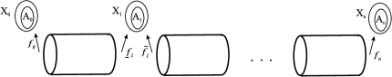
Figure 1:

Let us write formally $\underline{f_{0}}=\overline{f_{0}}=f_{0}$ and $\underline{f_{n}}=\overline{f_{n}}=f_{n}$. Now we suppose that for each $i=0,...,n$ and each $a\in A_{i}$, the point $a$ is identified with all points of the sets $\underline{f_{i}}^{-1}(a)$ and $\overline{f_{i}}^{-1}(a)$ and all other points of $Y$ with themselves. The quotient space which is obtained by this identification will be denoted by $X$.

The spaces $X_{i}$ and $Y_{i}\times\{t\},t\in(i-1,i)$ are homeomorphic to their embedded copies $\overline{X_{i}}$ and $\overline{Y_{i}}(t)$, called fibers of $X$ and these fibers make an ordered decomposition of $X$, called its fibrous decomposition and denoted by $X_{0}(Y_{1})...(Y_{n})X_{n}$. The number $n$ will be called the length of the corresponding fibrous decomposition. (When $n=0$, the decomposition reduces to $X_{0}$.)

Mapping each fiber $\overline{X_{i}}$ onto $i$ and each $\overline{Y_{i}}(t)$, $t\in(i-1,i)$ onto $t$, a function $\varphi:X\rightarrow[0,n]$ is defined and $\varphi^{-1}([0,k]),(k<n)$ is a subspace of $X$ whose fibrous decomposition is determined by the subsequences $(X_{0},A_{0}),...,(X_{k},A_{k}),Y_{1},...,Y_{k}$ and by the subset $\underline{f_{i}},\overline{f_{i}},i=0,...,k$ of the corresponding set of mappings. We call $\varphi$ a function associated with the given fibrous decomposition. (As it is seen, we use a terminology to avoid confusion with the existing one based on the morpheme ”fiber”).

A finite space $X$ will be called $0$-fibrous and the space $X$ itself will be considered as its own fibrous decomposition. Proceeding inductively, we call a topological space $m$-fibrous when it has a fibrous decomposition each fiber of which is $k$-fibrous for some $k\leq m-1$. Now we are ready to prove the statement that follows.

Theorem 2.2

Let $X$ be an $m$-fibrous space having its fibrous decomposition given by the sequences $(X_{0},A_{0}),(X_{1},A_{1}),...,(X_{n},A_{n})$ and $Y_{1},...,Y_{n}$ and the set of mappings $\underline{f_{i}},\overline{f_{i}},i=0,1,...,n$. Then, the Euler-Poincaré characteristic is defined for all spaces $X_{0},X_{1},...,X_{n}$ and $Y_{1},...,Y_{n}$ as well as for $X$ and

$$\chi(X)=\chi(X_{0})-\chi(Y_{1})+\chi(X_{1})-\cdots+\chi(X_{n-1})-\chi(Y_{n})+\chi(X_{n}).$$

Proof. The statement is trivially true when $m=0$. Let us suppose that it is true for all spaces which are $k$-fibrous for some $k\leq m-1$. Let $X$ be an $m$-fibrous space. When $X$ has a fibrous decomposition of the length $0$, then $X$ is $k$-fibrous for some $k\leq m-1$ and the statement is true. Let us suppose it is true for all $m$-fibrous spaces having a fibrous decomposition of the length less than $n$. Let $X$ be an $m$-fibrous space and let $(X_{0},A_{0}),(X_{1},A_{1}),...,(X_{n},A_{n})$ and $Y_{1},...,Y_{n}$ be sequences which, together with the set of mappings $\underline{f_{i}},\overline{f_{i}},i=0,1,...,n$ determine a fibrous decomposition of $X$. According to the definition of $m$-fibrous spaces, the spaces $X_{0},X_{1},...,X_{n}$ and $Y_{0},...,Y_{n}$ are $k$-fibrous for some $k\leq m-1$ and according to the inductive hypothesis on $m$, the E-P characteristic is defined for them.

Let $\varphi$ be the function associated with the fibrous decomposition of $X$. Modifying slightly Proposition 2.1, it is easily proved that $\varphi^{-1}([0,n-1])$ is a strong deformation retract of $\varphi^{-1}([0,n-1/3))$ as it is $\varphi^{-1}(n)$ of $\varphi^{-1}((n-2/3,n])$. As we have already noticed it, the E-P characteristic is defined for $\varphi^{-1}(n)\approx X_{n}$ and, according to the induction hypothesis on $n$, it is also defined for $\varphi^{-1}([0,n-1])$. From the following homotopy equivalences

$$\varphi^{-1}([0,n-1])\simeq\varphi^{-1}([0,n-1/3)),\varphi^{-1}(n)\simeq\varphi^{-1}((n-2/3,n])$$

it follows that E-P characteristic is also defined for the spaces $\varphi^{-1}([0,n-1/3))$ and $\varphi^{-1}((n-2/3,n])$. Being these two spaces open in $X$, we see that the triad

$$(X,\varphi^{-1}([0,n-1/3)),\varphi^{-1}((n-2/3,n]))$$

satisfies the excision property. Using now a very well known property of E-P characteristic (see, for example, [D]), we can write

$$\chi(X)=\chi(\varphi^{-1}([0,n-1/3)))+\chi(\varphi^{-1}(n-2/3,n]))-\chi(\varphi^{-1}((n-2/3,n-1/3)))$$

.

Since $\varphi^{-1}((n-2/3,n-1/3))\simeq Y_{n}$ and using previously established homotopy equivalences, we have

$$\chi(X)=\chi(\varphi^{-1}([0,n-1]))+\chi(\varphi^{-1}(n))-\chi(Y_{n}).$$

Using the induction hypothesis on $n$, we replace $\chi(\varphi^{-1}([0,n-1]))$ by the corresponding alternating sum, obtaining so the following equality

$$\chi(X)=(\chi(X_{0})-\chi(Y_{1})+\cdots+\chi(X_{n-1}))+\chi(X_{n})-\chi(Y_{n}).$$

Thus, we have proved all conclusions of Theorem 2.2.

3 Examples

First we prove a simple statement which is often useful when a quotient model of a space is replaced with a more convenient one defined on its subspace.

Let $X$ be a topological space and $\rho$ an equivalence relation on $X$. Let $A$ be a subset of $X$ such that for each $x\in X$, $[x]\cap A\neq\emptyset$, where $[x]$ is the equivalence class of $x$. Taking $A$ with its relative topology, the induced equivalence relation $\rho_{A}$ on $A$ determines the quotient space $A/\rho_{A}$. The model of the quotient space $A/\rho_{A}$ is simpler than that of $X/\rho$ and it is of some interest to know under which conditions these two quotient spaces are homeomorphic.

Let $p:X\rightarrow X/\rho$ and $p_{A}:A\rightarrow A/\rho_{A}$ be the natural projections and $i:A\rightarrow X$ and $j:A/\rho_{A}\rightarrow X/\rho$ the inclusions. Then, $p\circ i=j\circ p_{A}$. Being $p\circ i$ continuous and $p_{A}$ quotient, it follows that $j$ is also continuous. Being $j$ 1-1 and onto, $j^{-1}$ is also defined and we are looking for the conditions under which it is also continuous (and therefore, when $X\setminus A$ can be cut out from $X$).

Proposition 3.1

Let $(X,\rho)$ be a topological space with an equivalence relation on $X$. Let $A\subset X$ be such that for each $x\in X$, $[x]\cap A\neq\emptyset$ and let $\rho_{A}$ be the induced relation on $A$. If one of the following conditions

(i) $A$ is open and $p:X\rightarrow X/\rho$ is open,

(ii) $A$ is closed and $p:X\rightarrow X/\rho$ is closed,

(iii) $A$ is compact and $X/\rho$ is Hausdorff

holds true, then $A/\rho_{A}\approx X/\rho$.

Proof. Under (i), ((ii)) the mapping $p\circ i$ is open (closed) and onto. Hence, $p\circ i$ is quotient. From $j^{-1}\circ(p\circ i)=p_{A}$, it follows that $j^{-1}$ is continuous.

Under (iii), $p\circ i$ maps closed (compact) subsets of $A$ onto closed (compact) subsets of $X/\rho$. Hence, $p\circ i$ is quotient, what implies that $j^{-1}$ is continuous.

When we use $X_{0}(Y_{1})X_{1}...(Y_{n})X_{n}$ to denote a fibrous decomposition, then the fibers $\overline{X_{i}}$ are called transitional and $\overline{Y_{i}}(t)$ running.

Example 1. Let $X$ is a finite space having $n$ points. Then, $\chi(X)=n$.

Example 2. Let $X$ is a rosette of $n$ circles. Then, $\chi(X)=1-n$.

For a single copy of $S^{1}$, $\chi(S^{1})=1-2+1=0$. Let us suppose that E-P characteristic of a rosette of $n-1$ circles is $1-(n-1)$. Let $X_{0}$ be the subspace of $X$ that consists of $n-1$ circles.

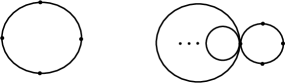
Figure 2:

A fibrous decomposition of $X$ is $X_{0}(2p)p$, where $p$ and $2p$ denote a one point and a two point space, respectively. Thus, we have

$$\chi(X)=\chi(X_{0})-2+1=1-(n-1)-2+1=1-n.$$

Following a similar proof, it is easy to see that for the space $X$ which is the sequence of touching circles $(x-2k)^{2}+y^{2}=1,k=0,1,...,n-1$, $\chi(X)=1-n$.

Example 3. When the boundary of an $n$-ball collapses to a point, an $n$-sphere $S^{n}$ is obtained and one of its fibrous decompositions is $p(S^{n-1})p$. From $\chi(S^{n})=1-\chi(S^{n-1})+1$, starting with $\chi(S^{0})=2$ and applying induction, one finds that $\chi(S^{n})$ is $2$ for $n$ even and $0$ for $n$ odd.

Example 4. The case of surfaces (both orientable and non-orientable) deserves a special attention. Here is a brief description of the corresponding fibrous decompositions while the detailed presentation of examples is postponed for Section 4.

Let $M_{g}$ be the surface which is $2$-sphere with $g$ holes (Fig. 3).

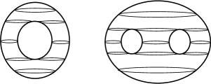
Figure 3:

A fibrous decomposition of $M_{g}$ is $p(S^{1})\dot{S}^{1}_{g+1}((g+1)S^{1})\dot{S}^{1}_{g+1}(S^{1})p$, where $\dot{S}^{1}_{g+1}$ is the sequence of $g+1$ touching circles (Example 2) and $(g+1)S^{1}$ disjoint topological sum of $g+1$ circles. Hence,

$$\chi(M_{g})=1-0+(-g)-0+(-g)-0+1=2-2g.$$

When $M_{g}$ is given as the quotient space obtained by identification of arcs of the boundary of a disc, following the command $\alpha_{1}\beta_{1}\alpha_{1}^{-1}\beta_{1}^{-1}...\alpha_{g}\beta_{g}\alpha_{g}^{-1}\beta_{g}^{-1}$, then $M_{g}$ has a fibrous decomposition $p(S^{1})\tilde{S^{1}}_{2g}$, where $\tilde{S^{1}}_{2g}$ is a rosette of $2g$ circles. Now, we have

$$\chi(M_{g})=1-0+(1-2g)=2-2g.$$

Identifying the opposite points of boundary circles of a disk, a disk with a circular hole, a disk with $2$ circular holes, etc. the surfaces $N_{1}$ (projective plane), $N_{2}$ (Klein bottle), $N_{3}$, etc. are obtained.

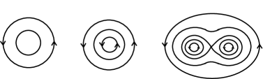
Figure 4:

Their fibrous decompositions are: $S^{1}(S^{1})p$, $S^{1}(S^{1})S^{1}$, $S^{1}(S^{1})\dot{S}^{1}_{2}(2S^{1})2S^{1}$, (where $\dot{S}^{1}_{2}$ are two touching circles), etc. Their E-P characteristics are

$$\chi(N_{1})=0-0+1=1,\chi(N_{2})=0-0+0=0,\chi(N_{3})=0-0+(-1)-0+0=-1,$$

etc. In the case of the surface $N_{h}$, one of its fibrous decompositions is

$$S^{1}(S^{1})\dot{S}^{1}_{h-1}((h-1)S^{1})(h-1)S^{1},$$

where $\dot{S}^{1}_{h-1}$ is a sequence of $h-1$ touching circles. Hence,

$$\chi(N_{h})=0-0+(1-(h-1))-0+0=2-h.$$

Taking $N_{h}$ as a quotient space obtained by identification of boundary points of a disk, following the command $\alpha_{1}^{2}...\alpha_{h}^{2}$, one of fibrous decompositions of $N_{h}$ is $p(S^{1})\tilde{S^{1}}_{h}$, where $\tilde{S^{1}}_{h}$ is the rosette of $h$ circles. Hence, $\chi(N_{h})=1-0+(1-h)=2-h$.

Example 5. Let $\mathbb{R}P^{n}$ be $n$-dimensional real projective space obtained when antipodal points of the boundary of an $n$-ball $B^{n}$ are identified. The quotient space obtained by this identification on the boundary $S^{n-1}$ of $B^{n}$ is $(n-1)$-dimensional real projective space, what is easily seen when open south hemisphere is cut out and Proposition 3 applied. Thus, a fibrous decomposition of $\mathbb{R}P^{n}$ is $p(S^{n-1})\mathbb{R}P^{n-1}$ and

$$\chi(\mathbb{R}P^{n})=1-\chi(S^{n-1})+\chi(\mathbb{R}P^{n-1}).$$

Starting with $\chi(S^{0})=2$ and $\chi(\mathbb{R}P^{0})=1$, it follows that $\chi(\mathbb{R}P^{n})$ is $1$ for $n$ even and $0$ for $n$ odd.

Example 6. According to the way how $n$-dimensional dunce hat $D^{n}$ is obtained from $n$-dimensional simplex by the identification of points on its boundary (see [AMS]), the space $D^{n}$ has a fibrous decomposition $p(S^{n-1})D^{n-1}$, whence

$$\chi(D^{n})=1-\chi(S^{n-1})+\chi(D^{n-1}).$$

From this equality it easily follows that $\chi(D^{n})$ is $1$ for $n$ even and $0$ for $n$ odd.

Example 7. Identifying the opposite $2$-faces of the cube $I^{3}=[0,1]\times[0,1]\times[0,1]$, pairs of points $(0,y,z),(1,y,z);(x,0,z),(x,1,z)and(x,y,0),(x,y,1)$ are identified and a $3$-dimensional torus $T^{3}$ is obtained. Now we calculate directly E-P characteristic of $T^{3}$ (and as it is a very well known fact, each manifold of odd dimension has its E-P characteristic equal $0$).

An obvious fibrous decomposition of $T^{3}$ is $T^{2}(2T^{2})T^{2}$ (see Fig. 5) and thus, $\chi(T^{3})=0-0+0=0$.

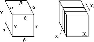
Figure 5:

Example 8. Let $K$ be a finite $n$-dimensional CW-complex. Starting with the centers of $n$-cells, a fibrous decomposition of $K$ is $\alpha_{n}p(\alpha_{n}S^{n-1})K^{n-1}$, where $\alpha_{n}$ is the number of $n$-cells of $K$ and $K^{n-1}$ is $(n-1)$-skeleton of $K$. From that decomposition, applying induction, it easily follows that $K$ is an $n$-fibrous space and from $\chi(K)=\alpha_{n}-\alpha_{n}\chi(S^{n-1})+\chi(K^{n-1})$ that $\chi(K)=\sum(-1)^{i}\alpha_{i}$, where $\alpha_{i}$ is the number of $i$-cells of $K$.

4 Euler characteristic of surfaces

More technical aspects of fibrous decompositions of surfaces are presented in Example 4, in the previous section. Here we emphasize that the models of $2$-surfaces, which represent their decompositions into lines, serve for easy calculation of the Euler-Poincaré characteristic and at the same time they enrich our geometric imagination.

Recall that traditionally the Euler characteristic is defined for topological spaces which are homeomorphic to (finite) simplicial complexes and calculated as $\chi(X)=\sum f_{i}$, where $f_{i}$ is the number of $i$-dimensional faces of the complex.

Here the calculation proceeds without triangulation and, speaking figuratively, just by decomposing curves into points, surfaces into curves, bodies into surfaces, etc.

Figure 6: The sphere $M_{0}$ and the torus $M_{1}$

(a) Orientable surfaces $M_{g}$ (spheres with $g$ holes). The $2$-sphere and the torus ($\chi(M_{0})=2,\chi(M_{1})=0$ ) are exhibited in Figure 6. The general case ($\chi(M_{g})=2-2g$) is depicted in Figure 7.

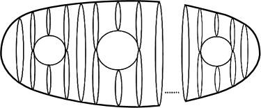
Figure 7: The $2$-sphere with $g$-holes

Figure 8: Projective plane $M_{0}^{\prime}$ and the non-orientable surface $M_{1}^{\prime}$

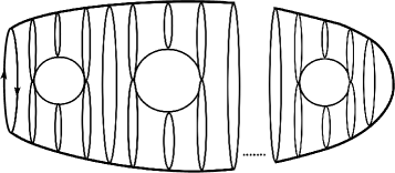
Figure 9: Non-orientable surface $M_{g}^{\prime}$ with $g$-holes

Figure 10: Klein bottle $M_{0}^{\prime\prime}$ and the non-orientable surface $M_{1}^{\prime\prime}$

Figure 11: Non-orientable surface $M_{g}^{\prime\prime}$ with $g$-holes

(b) Non-orientable surfaces $M_{g}^{\prime}$ arise when a spherical cap is cut off along a circle whose diametrally opposite points are identified. The projective plane $M_{0}^{\prime}$ and the non-orientable surface $M_{1}^{\prime}$ ($\chi(M_{0}^{\prime})=1,\chi(M_{1}^{\prime})=-1$ ) are exhibited in Figure 8. The general case ($\chi(M_{g}^{\prime})=1-2g$) is depicted in Figure 9.

(c) Non-orientable surfaces $M_{g}^{\prime\prime}$ arise when two opposite spherical caps are removed and the corresponding boundary circles are identified. The Klein bottle $M_{0}^{\prime\prime}$ and the non-orientable surface $M_{1}^{\prime\prime}$ ($\chi(M_{0}^{\prime\prime})=0,\chi(M_{1}^{\prime\prime})=-2$) are exhibited in Figure 10. The general case ($\chi(M_{g}^{\prime\prime})=-2g$) is depicted in Figure 11.

References

- [AMS] R. N. Anderson, M. M. Marjanović, R. M. Schori. Symetric products and higher dimensional dunce hats. Topology Proceedings, 18, 1993, 7–17.
- [CGR] J. Curry, R. Ghrist, M. Robinson. Euler Calculus with Applications to Signals and Sensing. arXiv:1202.0275v1 [math.AT], February 1, 2012.
- [D] A. Dold. Lectures on Algebraic Topology. Springer-Verlag, 1972.
- [FLS] T. M. Fiore, W. Lück, R. Sauer. Euler Characteristics of Categories and Homotopy Colimits arXiv:1007.3868v3 [math.AT], March 25, 2011.
- [M] M. M. Marjanović. Metric Euclidean projective and topological properties. The Teaching of Mathematics, IV (1), 2001, 41–70. (http://elib.mi.sanu.ac.rs/journals/tm).
- [V] O. Viro. Some integral calculus based on Euler characteristic. Lecture Notes in Mathematics, 1346, 1988, 127–138.