Dynamics of rogue waves in the Davey-Stewartson II equation

Abstract

General rogue waves in the Davey-Stewartson-II equation are derived by the bilinear method, and the solutions are given through determinants. It is shown that the simplest (fundamental) rogue waves are line rogue waves which arise from the constant background in a line profile and then retreat back to the constant background again. It is also shown that multi-rogue waves describe the interaction between several fundamental rogue waves, and higher-order rogue waves exhibit different dynamics (such as rising from the constant background but not retreating back to it). A remarkable feature of these rogue waves is that under certain parameter conditions, these rogue waves can blow up to infinity in finite time at isolated spatial points, i.e., exploding rogue waves exist in the Davey-Stewartson-II equation.

I Introduction

Rogue waves are large and spontaneous nonlinear waves and have been found in a variety of physical systems (such as the ocean and optical systems) rogue_water ; Rogue_nature1 . Rogue waves generally occur due to modulation instability of monochromatic waves. One of the simplest mathematical models for modulation instability is the nonlinear Schrödinger (NLS) equation. For this equation, explicit expressions of rogue-wave solutions have been obtained by a variety of techniques such as the Darboux transformation, the bilinear method and so on Peregrine ; Akhmediev_PRE ; Rogue_higher_order ; Rogue_higher_order2 ; Rogue_Gaillard ; Rogue_triplet ; Rogue_circular ; Liu_qingping ; OY . These NLS rogue waves can also be obtained from homoclinic solutions of the NLS equation under certain limits Akhmediev_1985 ; Akhmediev_1988 ; Its_1988 ; Ablowitz_homo ; Rogue_homo , or from rational solutions of the Davey-Stewartson equation through dimension reductions OY ; Ablowitz_private . Physically these NLS rogue waves have been observed in optical fibers and water tanks Rogue_nature2 ; NLS_rogue_water . In addition to the NLS equation, rogue waves have also been obtained in other wave equations, such as the Hirota equation, the derivative NLS equation and the Davey-Stewartson-I equation rogue_Hirota ; rogue_DNLS1 ; rogue_DNLS2 ; OY_DSI . Explicit rogue-wave solutions in mathematical model equations reveal the conditions for rogue-wave formation and facilitate the observation and prediction of rogue waves in physical systems rogue_water ; Rogue_nature1 ; Rogue_nature2 ; NLS_rogue_water .

In this article, we derive general rogue-wave solutions in the Davey-Stewartson-II equation. This equation arises in the modeling of two-dimensional shallow water waves Benney_Roskes ; Davey_Stewartson ; Ablowitz_book . Our derivation uses the bilinear method, and the solutions are expressed in terms of determinants. We show that the simplest (fundamental) rogue waves are line rogue waves which arise from the constant background in a line profile and then retreat back to the constant background again. We also show that the interaction between several fundamental rogue waves are described by multi-rogue-wave solutions. However, higher-order rogue waves are found to exhibit different dynamics, such as rising from the constant background but not retreating back to it. An important feature about these rogue waves is that, under certain parameter conditions, these waves can blow up to infinity in finite time at isolated spatial points (we call such solutions exploding rogue waves). The existence of exploding rogue waves is remarkable, and their appearance can be catastrophic in physical systems.

It is noted that rogue waves are rational solutions of nonlinear systems in general. For the Davey-Stewartson equations, certain types of rational solutions have been derived before SA . Those rational solutions, under parameter restrictions, would yield multi-rogue waves (see Sec. III.2 of this article). The rational solutions we would derive (in the next section), on the other hand, are more general; and these rational solutions, under parameter restrictions, could yield not only multi-rogue waves but also higher-order rogue waves.

II Rational solutions in the Davey-Stewartson-II equation

Evolution of a two-dimensional wavepacket on water of finite depth is governed by the Benney-Roskes-Davey-Stewartson equation Benney_Roskes ; Davey_Stewartson ; Ablowitz_book . In the shallow-water (or long-wave) limit, this equation is integrable (see Ablowitz_book2 and the references therein). This integrable equation is sometimes just called the Davey-Stewartson (DS) equation in the literature. The DS equation is divided into two types, DSI and DSII equations, depending on whether the surface tension is strong or weak Ablowitz_book .

In this paper, we study the DSII equation. The normalized form of this equation is

$$\begin{array}[]{l}iA_{t}=A_{xx}-A_{yy}+(\epsilon|A|^{2}-2Q)A,\\[5.0pt] Q_{xx}+Q_{yy}=\epsilon(|A|^{2})_{xx},\end{array}$$ (2.1)

where $\epsilon=1$ or $-1$. Through the variable transformation

$$A=\sqrt{2}\,\frac{g}{f},\quad Q=\epsilon-(2\log f)_{xx},$$ (2.2)

where $f$ is a real variable and $g$ a complex one, this equation is transformed into the bilinear form,

$$\begin{array}[]{l}(D_{x}^{2}-D_{y}^{2}-iD_{t})g\cdot f=0,\\[5.0pt] (D_{x}^{2}+D_{y}^{2})f\cdot f=2\epsilon(f^{2}-|g|^{2}).\end{array}$$ (2.3)

Rogue waves are rational solutions under certain parameter restrictions. Thus we first present general rational solutions to the DSII equation in the following theorem. The proof of this theorem is given in Appendix A.

Theorem 1  The DSII equation (2.1) admits rational solutions (2.2) with $f$ and $g$ given by $2N\times 2N$ determinants

$$f=\tau_{0},\quad g=\tau_{1},$$ (2.4)

where

$$\tau_{n}=\left|\begin{matrix}m_{ij}^{(n)}&\widehat{m}_{ij}^{(n)}\cr\vskip 5.0pt\cr\displaystyle\epsilon\hskip 1.42271pt\overline{\widehat{m}_{ij}^{(-n)}}&\displaystyle\overline{m_{ij}^{(-n)}}\end{matrix}\right|,$$ (2.5)

$$m_{ij}^{(n)}=\sum_{k=0}^{n_{i}}c_{ik}(p_{i}\partial_{p_{i}}+\xi^{\prime}_{i}+n)^{n_{i}-k}\sum_{l=0}^{m_{j}}d_{jl}(q_{j}\partial_{q_{j}}+\eta^{\prime}_{j}-n)^{m_{j}-l}\frac{1}{p_{i}+q_{j}},$$ (2.6)

$$\widehat{m}_{ij}^{(n)}=\sum_{k=0}^{n_{i}}c_{ik}(p_{i}\partial_{p_{i}}+\xi^{\prime}_{i}+n)^{n_{i}-k}\sum_{l=0}^{m_{j}}\bar{d}_{jl}(\bar{q}_{j}\partial_{\bar{q}_{j}}+\overline{\eta^{\prime}_{j}}+n)^{m_{j}-l}\frac{1}{p_{i}\bar{q}_{j}+\epsilon},$$ (2.7)

$$\xi^{\prime}_{i}=\frac{p_{i}-\epsilon/p_{i}}{2}x+\frac{p_{i}+\epsilon/p_{i}}{2}\sqrt{-1}\hskip 1.70709pty+\frac{p_{i}^{2}+1/p_{i}^{2}}{\sqrt{-1}}t,$$ (2.8)

$$\eta^{\prime}_{j}=\frac{q_{j}-\epsilon/q_{j}}{2}x+\frac{q_{j}+\epsilon/q_{j}}{2}\sqrt{-1}\hskip 1.70709pty-\frac{q_{j}^{2}+1/q_{j}^{2}}{\sqrt{-1}}t,$$ (2.9)

the overbar ‘$\ \bar{}\$’ represents complex conjugation, $i,j=1,\dots,N$, $n_{i},m_{j}$ are arbitrary non-negative integers, and $p_{i},q_{j},c_{ik},d_{jl}$ are arbitrary complex constants.

Remark 1.   By a scaling of $f$ and $g$, we can normalize $c_{i0}=d_{j0}=1$ without loss of generality, thus hereafter we set $c_{i0}=d_{j0}=1$.

Remark 2.  For $\epsilon=-1$, $f$ in (2.4) is non-negative, i.e., $f\geq 0$. A proof is given in Appendix B. Since $f$ is the denominator of the solutions $A$ and $Q$, the above rational solutions are nonsingular as long as $f>0$. But it is also possible that $f$ hits zero and the corresponding solution blows up to infinity at a certain point of space-time, which we will see later.

Remark 3. Rational solutions in the DS equations have been derived in SA before. The nonsingular rational solutions for the DSII equation in that paper correspond to special rational solutions in the above theorem with $n_{1}=\cdots=n_{N}=1$ and $m_{1}=\cdots=m_{N}=0$.

The simplest rational solution is obtained when $N=1$, $n_{1}=1$ and $m_{1}=0$. In this case,

$$\tau_{n}=\left|\begin{matrix}m_{11}^{(n)}&\widehat{m}_{11}^{(n)}\cr\vskip 5.0pt\cr\displaystyle\epsilon\hskip 1.42271pt\overline{\widehat{m}_{11}^{(-n)}}&\displaystyle\overline{m_{11}^{(-n)}}\end{matrix}\right|,$$

where

$$m_{11}^{(n)}=\frac{1}{p_{1}+q_{1}}\Big{(}\xi_{1}^{\prime}+n-\frac{p_{1}}{p_{1}+q_{1}}+c_{11}\Big{)},$$

$$\widehat{m}_{11}^{(n)}=\frac{1}{p_{1}\bar{q}_{1}+\epsilon}\Big{(}\xi_{1}^{\prime}+n-\frac{p_{1}\bar{q}_{1}}{p_{1}\bar{q}_{1}+\epsilon}+c_{11}\Big{)},$$

and $\xi_{1}^{\prime}$ is defined in (2.8). This solution seems to have three free complex parameters $p_{1}$, $q_{1}$ and $c_{11}$, but $q_{1}$ can be absorbed into $c_{11}$ by a reparametrization. Indeed, by defining

$$\theta=c_{11}-\frac{p_{1}}{(|p_{1}|^{2}-\epsilon)(|q_{1}|^{2}-\epsilon)}\left(\frac{|p_{1}\bar{q}_{1}+\epsilon|^{2}}{p_{1}+q_{1}}-\frac{\epsilon\hskip 1.13791pt\bar{q}_{1}|p_{1}+q_{1}|^{2}}{p_{1}\bar{q}_{1}+\epsilon}\right),$$

and denoting $p_{1}=p$, $\xi_{1}^{\prime}+\theta=\xi$, we can show that the terms in $\tau_{n}$ which are linear in $\xi+n$ and $\bar{\xi}-n$ vanish, and this $\tau_{n}$ reduces to

$$\tau_{n}=(\xi+n)(\overline{\xi}-n)+\Delta,$$

$$\xi=ax+by+\omega t+\theta,\quad\Delta=\frac{-\epsilon|p|^{2}}{(|p|^{2}-\epsilon)^{2}},$$

$$a\equiv\frac{p-\epsilon/p}{2},\quad b\equiv\frac{p+\epsilon/p}{2}i,\quad\omega\equiv\frac{p^{2}+1/p^{2}}{i},$$

up to a constant multiplication, thus this new $\tau_{n}$ yields the same solution. The solution from this new $\tau_{n}$ has only two independent complex parameters $p$ and $\theta$ now. If we separate the real and imaginary parts of $a,b,\omega$ and $\theta$ as

$$a=a_{1}+ia_{2},\hskip 5.69046ptb=b_{1}+ib_{2},\hskip 5.69046pt\omega=\omega_{1}+i\omega_{2},\hskip 5.69046pt\theta=\theta_{1}+i\theta_{2},$$

then the explicit expressions for this solution are

$$A(x,y,t)=\sqrt{2}\left[1-\frac{2i(a_{2}x+b_{2}y+\omega_{2}t+\theta_{2})+1}{f}\right].$$ (2.10)

$$Q(x,y,t)=\epsilon-(2\log f)_{xx},$$ (2.11)

where

$$f=(a_{1}x+b_{1}y+\omega_{1}t+\theta_{1})^{2}+(a_{2}x+b_{2}y+\omega_{2}t+\theta_{2})^{2}+\Delta.$$

This simplest rational solution is nonsingular when $\epsilon=-1$ (where $\Delta>0$). In this case, the solution exhibits two distinctly different dynamics depending on the parameter value of $p$.

1. If $|p|\neq 1$, then it is easy to see that $b/a$ is not real, hence $b_{1}/b_{2}\neq a_{1}/a_{2}$. In this case, along the $[x(t),y(t)]$ trajectory where

   $$a_{1}x+b_{1}y=-\omega_{1}t,\quad a_{2}x+b_{2}y=-\omega_{2}t,$$

   solutions $(A,Q)$ are constants. In addition, at any given time, $(A,Q)\to(\sqrt{2},\epsilon)$ when $(x,y)$ goes to infinity. Thus the solution is a two-dimensional lump moving on a constant background SA .

2. If $|p|=1$, then $a,b$ are real but $\omega$ is imaginary. In this case, the solution depends on $(x,y)$ through the combination $a_{1}x+b_{1}y$ and is thus a line wave. As $t\to\pm\infty$, this line wave goes to a uniform constant background (as long as $p^{2}\neq\pm i$); in the intermediate times, it rises to a higher amplitude. Thus this line wave is a line rogue wave which “appears from nowhere and disappears with no trace”.

When $\epsilon=1$, the rational solution (2.10)-(2.11) is singular on a certain elliptic curve in the $(x,y)$ plane for any time $t$, since $\Delta<0$ now. For this $\epsilon$, the constant-background solution is modulationally stable Tajiri_1999 , thus no rogue waves can be expected. In view of this, we only consider the case of $\epsilon=-1$ in the remainder of the paper.

III Rogue waves in the Davey-Stewartson-II equation

As we see from the above analysis, rogue waves would result from the rational solutions in Theorem 1 for $\epsilon=-1$ under certain parameter conditions. Specifically, to obtain rogue waves, we need to require $\epsilon=-1$ and

$$|p_{j}|=1,\ \mbox{if}\ n_{j}>0;\quad|q_{j}|=1,\ \mbox{if}\ m_{j}>0;\quad 1\leq j\leq N.$$ (3.1)

In this section, we examine the dynamics of these rogue waves in detail.

III.1 Fundamental rogue waves

Fundamental rogue waves in the DSII equation are obtained when one takes

$$\epsilon=-1,\ N=1,\ n_{1}=1,\ m_{1}=0,\ p_{1}=e^{i\beta}$$ (3.2)

in the rational solution (2.4), with $\beta$ being a real parameter and $p_{1}^{2}\neq\pm i$ (i.e., $\cos 2\beta\neq 0$). As we have explained in the previous section, this solution is equivalent to (2.10)-(2.11). After a shift of time and space coordinates, $\theta_{1}$ and $\theta_{2}$ can be eliminated. Then in view of $p=e^{i\beta}$, this fundamental rogue wave becomes

$$A(x,y,t)=\sqrt{2}\left(1-\frac{4-16it\cos 2\beta}{1+4(x\cos\beta-y\sin\beta)^{2}+16t^{2}\cos^{2}2\beta}\right),$$ (3.3)

$$Q(x,y,t)=-1-16\cos^{2}\beta\frac{1-4(x\cos\beta-y\sin\beta)^{2}+16t^{2}\cos^{2}2\beta}{[1+4(x\cos\beta-y\sin\beta)^{2}+16t^{2}\cos^{2}2\beta]^{2}},$$ (3.4)

where $\beta$ is a free real parameter. This solution describes a line wave with the line oriented in the ($\sin\beta,\cos\beta$) direction of the $(x,y)$ plane, and the orientation angle is $\pi/2-\beta$. The width of this line wave is the same for all $\beta$ values, i.e., the width is angle-independent. At any given time, this solution is a constant along the line direction (with fixed $x\cos\beta-y\sin\beta$) and approaches the constant background away from the center of the line (with $x\cos\beta-y\sin\beta\to\pm\infty$). When $t\to\pm\infty$, the solution $A$ uniformly approaches the constant background $\sqrt{2}$; but in the intermediate times, $|A|$ reaches maximum amplitude $3\sqrt{2}$ (i.e., three times the background amplitude) at the center ($x\cos\beta-y\sin\beta=0$) of the line wave at time $t=0$. The speed at which this line wave climbs to its peak amplitude is proportional to $|\cos 2\beta|$, which is angle-dependent. This fundamental rogue wave is illustrated in Fig. 1 with $\beta=\pi/6$.

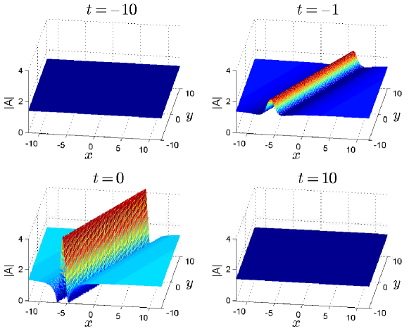
Figure 1: A fundamental rogue wave (3.3) with $\beta=\pi/6$.

It is noted that under the same parameter conditions (3.2) but with $\cos 2\beta=0$, i.e., this line wave is oriented diagonally ($45^{\circ}$) or anti-diagonally ($-45^{\circ}$), then $\omega=0$ in the rational solution (2.10)-(2.11). In this case, after a shift of space coordinates, $\theta_{1}$ can be eliminated. Hence this rational solution becomes

$$A(x,y,t)=\sqrt{2}\left(1-\frac{4+8i\theta_{2}}{1+2(x\pm y)^{2}+4\theta_{2}^{2}}\right),$$ (3.5)

$$Q(x,y,t)=-1-8\frac{1-2(x\pm y)^{2}+4\theta_{2}^{2}}{[1+2(x\pm y)^{2}+4\theta_{2}^{2}]^{2}},$$ (3.6)

where $\theta_{2}$ is a free real parameter. This solution is not a rogue wave. Instead, it is a stationary line soliton sitting on the constant background. Its peak $|A|$ amplitude is $\sqrt{2(9+4\theta_{2}^{2})/(1+4\theta_{2}^{2})}$. The highest value of this peak amplitude is $3\sqrt{2}$ (three times the constant background), which is attained at $\theta_{2}=0$. When $|\theta_{2}|$ increases to infinity, this peak amplitude decreases to the background amplitude $\sqrt{2}$.

If $N>1$, or $N=1$ but $m_{1}+n_{1}>1$, the rational solutions in Theorem 1 under parameter restriction (3.1) will give a wide variety of non-fundamental rogue waves. For simplicity, we consider three subclasses of such solutions below.

III.2 Multi-rogue waves

One subclass of non-fundamental rogue waves is the multi-rogue waves which describe the interaction between several fundamental rogue waves. These solutions can be obtained from Theorem 1 by taking

$$\epsilon=-1,\quad N>1,\quad n_{j}=1,\quad m_{j}=0,\quad p_{j}=e^{i\beta_{j}},\quad 1\leq j\leq N,$$ (3.7)

where $\beta_{j}$ is a free real parameter (with $\cos 2\beta_{j}\neq 0$). In this case, the $\tau$-solution (2.5) becomes

$$\tau_{n}=\left|\begin{matrix}m_{ij}^{(n)}&\widehat{m}_{ij}^{(n)}\cr\vskip 5.0pt\cr\displaystyle-\hskip 1.42271pt\overline{\widehat{m}_{ij}^{(-n)}}&\displaystyle\overline{m_{ij}^{(-n)}}\end{matrix}\right|,$$ (3.8)

where

$$m_{ij}^{(n)}=\frac{1}{p_{i}+q_{j}}\Big{(}\xi_{i}^{\prime}+n-\frac{p_{i}}{p_{i}+q_{j}}+c_{i1}\Big{)},$$ (3.9)

$$\widehat{m}_{ij}^{(n)}=\frac{1}{p_{i}\bar{q}_{j}-1}\Big{(}\xi_{i}^{\prime}+n-\frac{p_{i}\bar{q}_{j}}{p_{i}\bar{q}_{j}-1}+c_{i1}\Big{)},$$ (3.10)

$\xi_{i}^{\prime}$ is defined in (2.8), and $q_{j},c_{i1}$ are free complex constants (but with $q_{j}\neq\pm p_{i}$ to avoid zero divisors). When $t\to\pm\infty$, the solutions $(A,Q)$ approach the constant background uniformly in the entire $(x,y)$ plane. In the intermediate times, $N$ fundamental line rogue waves arise from the constant background, interact with each other, and then disappear into the background again. Depending on the parameter choices, individual line rogue waves can reach their peak amplitudes at the same time or at different times, with the former yielding stronger interactions.

Now we illustrate these multi-rogue waves and examine their dynamics. To obtain a two-rogue wave solution, we take parameter values

$$N=2,\quad p_{1}=1,\quad p_{2}=i,\quad q_{1}=0,\quad q_{2}=-3,\quad c_{11}=0,\quad c_{21}=i/2.$$ (3.11)

The corresponding solution $|A|$ is displayed in Fig. 2. It is seen that as $t\to\pm\infty$, the solution uniformly approaches the constant background $\sqrt{2}$; but in the intermediate times, a cross-shape rogue wave appears. This cross rogue wave describes the interaction between two fundamental line rogue waves, one oriented along the $y$ direction (corresponding to the parameter $p_{1}$), and the other one oriented along the $x$ direction (corresponding to the parameter $p_{2}$). These two individual line waves reach their peak amplitude $3\sqrt{2}$ at different times, with the $x$-direction one peaking at $t\approx-1/4$ and the $y$-direction one peaking at $t\approx 0$.

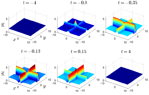
Figure 2: A two-rogue wave solution (3.8) with parameters (3.11).

Next, we take parameter values

$$N=4,\ p_{1}=1,\ p_{2}=e^{i/2},\ p_{3}=e^{i},\ p_{4}=e^{2i},\ q_{1}=-0.1,\ q_{2}=0,$$ (3.12)

$$q_{3}=0.1,\ q_{4}=0.2,\ c_{11}=-2i,\ c_{21}=0,\ c_{31}=2i,\ c_{41}=i/2,$$ (3.13)

which gives a four-rogue wave solution. This solution ($|A|$) is displayed in Fig. 3. As $t\to\pm\infty$, the solution uniformly goes to the constant background $\sqrt{2}$; but in the intermediate times, a rogue wave comprising four lines emerges. These four individual line waves reach their peak amplitudes $3\sqrt{2}$ at approximately the same time $t=0$, and their widths are identical (see $t=0$ panel). Due to the interaction of these four line waves, the maximum amplitude of the solution (at intersections of the four lines) can be very high. Indeed, at $t=-1$, we find that the peak amplitude of the solution $|A|$ reaches approximately $30\sqrt{2}$ (i.e., 30 times the constant background). Thus such rogue waves can be fairly dangerous if they arise in physical situations.

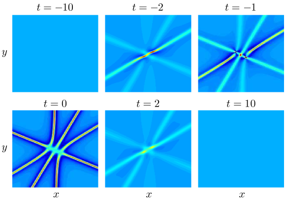
Figure 3: A four-rogue wave solution (3.8) with parameters (3.12)-(3.13). Plotted is the $|A|$ field, with red color indicating higher values. The spatial region in each panel is $-20\leq x,y\leq 20$, and the constant-background value is $\sqrt{2}$.

In the general $N$-rogue wave solution (3.8), $\beta_{j}$ is a free real parameter, and $q_{j},c_{j1}$ are free complex parameters ($1\leq j\leq N$). Thus it appears that this $N$-rogue-wave solution contains $N$ free real parameters and $2N$ free complex parameters, totaling $5N$ free real parameters. But these parameters are reducible (similar to the simplest rational solutions in the previous section). Indeed, when $N=2$, by a reparametrization of

$$\widehat{c}_{i1}=c_{i1}-p_{i}\Big{\{}\sum_{j=1}^{2}\Big{(}\frac{1}{p_{i}+q_{j}}+\frac{\bar{q}_{j}}{p_{i}\bar{q}_{j}-1}-\frac{1}{p_{i}+p_{j}}\Big{)}-\frac{1}{p_{i}-p_{3-i}}\Big{\}},\quad i=1,2,$$

we can show that the two-rogue-wave solution (3.8) is reduced to

$$\begin{array}[]{l}\displaystyle\tau_{n}=\Big{(}(\zeta_{1}+n)(\zeta_{2}+n)-\frac{1}{|p_{1}-p_{2}|^{2}}\Big{)}\Big{(}(\bar{\zeta}_{1}-n)(\bar{\zeta}_{2}-n)-\frac{1}{|p_{1}-p_{2}|^{2}}\Big{)}\\[5.0pt] \quad\displaystyle+\sum_{i=1}^{2}\sum_{j=1}^{2}\frac{1}{|p_{3-i}+p_{3-j}|^{2}}(\zeta_{i}+n)(\bar{\zeta}_{j}-n)+\frac{1}{2}\frac{1}{|p_{1}+p_{2}|^{2}}+\frac{1}{16}\Big{|}\frac{p_{1}-p_{2}}{p_{1}+p_{2}}\Big{|}^{4}\end{array}$$ (3.14)

up to a constant multiplication (which does not affect the solution). Here $\zeta_{i}=\xi^{\prime}_{i}+\widehat{c}_{i1},\quad i=1,2$. In this equivalent $\tau_{n}$ solution, parameters $q_{j}$ disappear, thus it contains only $\beta_{1}$, $\beta_{2}$, $\widehat{c}_{11}$ and $\widehat{c}_{21}$. Of the two complex constants $\widehat{c}_{11}$ and $\widehat{c}_{21}$, their real parts and the imaginary part of one of them can be further normalized to be zero by a shift of the $(x,y,t)$ axes. Thus this two-rogue wave solution contains only three irreducible real parameters. For the general $N$-rogue wave solution (3.8), we conjecture that all $q_{j}$ parameters can also be removed by a reparametrization of $c_{i1}$, hence this $N$-rogue wave solution contains only $3(N-1)$ irreducible real parameters (after a shift of $(x,y,t)$).

It is noted that if instead of (3.7), one takes

$$N>1,\quad n_{1}=n_{2}=\dots=n_{N}=0,\quad m_{1}=m_{2}=\dots=m_{N}=1,$$

then the same multi-rogue-wave solutions as above will be obtained. Thus different parameter choices can lead to the same solutions.

III.3 Higher-order rogue waves

A second subclass of non-fundamental rogue waves is the higher-order rogue waves. These solutions are obtained from Theorem 1 by taking

$$\epsilon=-1,\quad N=1,\quad n_{1}>1,\quad m_{1}=0,\quad|p_{1}|=1.$$ (3.15)

In this case, the $\tau$-solution (2.5) becomes

$$\tau_{n}=\left|\begin{matrix}m_{11}^{(n)}&\widehat{m}_{11}^{(n)}\cr\vskip 5.0pt\cr\displaystyle-\hskip 1.42271pt\overline{\widehat{m}_{11}^{(-n)}}&\displaystyle\overline{m_{11}^{(-n)}}\end{matrix}\right|,$$ (3.16)

where

$$m_{11}^{(n)}=\sum_{k=0}^{n_{1}}c_{1k}(p_{1}\partial_{p_{1}}+\xi^{\prime}_{1}+n)^{n_{1}-k}\frac{1}{p_{1}+q_{1}},$$ (3.17)

$$\widehat{m}_{11}^{(n)}=\sum_{k=0}^{n_{1}}c_{1k}(p_{1}\partial_{p_{1}}+\xi^{\prime}_{1}+n)^{n_{1}-k}\frac{1}{p_{1}\bar{q}_{1}-1},$$ (3.18)

$\xi_{i}^{\prime}$ is defined in (2.8), $c_{10}=1$, and $c_{1k},q_{1}$ are free complex constants. These higher-order rogue waves exhibit dynamics different from those of multi-rogue waves, as we will demonstrate below.

For simplicity, we consider second-order rogue waves where $n_{1}=2$. In this case, we find that

$$m_{11}^{(n)}=\frac{1}{p_{1}+q_{1}}\Big{\{}\Big{(}\xi_{1}^{\prime}+n-\frac{p_{1}}{p_{1}+q_{1}}+\frac{c_{11}}{2}\Big{)}^{2}+\xi_{1}^{\prime\prime}+c_{12}-\frac{c_{11}^{2}}{4}-\frac{p_{1}q_{1}}{(p_{1}+q_{1})^{2}}\Big{\}},$$

$$\widehat{m}_{11}^{(n)}=\frac{1}{p_{1}\bar{q}_{1}-1}\Big{\{}\Big{(}\xi_{1}^{\prime}+n-\frac{p_{1}\bar{q}_{1}}{p_{1}\bar{q}_{1}-1}+\frac{c_{11}}{2}\Big{)}^{2}+\xi_{1}^{\prime\prime}+c_{12}-\frac{c_{11}^{2}}{4}+\frac{p_{1}\bar{q}_{1}}{(p_{1}\bar{q}_{1}-1)^{2}}\Big{\}},$$

where

$$\xi_{1}^{\prime\prime}\equiv p_{1}\partial_{p_{1}}\xi_{1}^{\prime}=\frac{p_{1}-1/p_{1}}{2}x+\frac{p_{1}+1/p_{1}}{2}\sqrt{-1}\hskip 1.70709pty+\frac{p_{1}^{2}-1/p_{1}^{2}}{\sqrt{-1}}\hskip 1.42271pt2t.$$

Denoting

$$p=p_{1},\quad q=q_{1},\quad\xi=\xi_{1}^{\prime}+a,\quad\zeta=\xi_{1}^{\prime\prime}+b,$$

where $a\equiv c_{11}/2-1$ and $b\equiv c_{12}-c_{11}^{2}/4$, the $\tau_{n}$ solution (3.16) becomes

$$\tau_{n}=\frac{1}{|p+q|^{2}}\Big{\{}\Big{(}\xi+n+\frac{q}{p+q}\Big{)}^{2}+\zeta-\frac{pq}{(p+q)^{2}}\Big{\}}\Big{\{}\Big{(}\bar{\xi}-n+\frac{\bar{q}}{\bar{p}+\bar{q}}\Big{)}^{2}+\bar{\zeta}-\frac{\bar{p}\bar{q}}{(\bar{p}+\bar{q})^{2}}\Big{\}}$$

$$\qquad+\frac{1}{|p\bar{q}-1|^{2}}\Big{\{}\Big{(}\xi+n-\frac{1}{p\bar{q}-1}\Big{)}^{2}+\zeta+\frac{p\bar{q}}{(p\bar{q}-1)^{2}}\Big{\}}\Big{\{}\Big{(}\bar{\xi}-n-\frac{1}{\bar{p}q-1}\Big{)}^{2}+\bar{\zeta}+\frac{\bar{p}q}{(\bar{p}q-1)^{2}}\Big{\}}.$$

This solution has four apparent complex parameters, $p,q,a$ and $b$. But $q$ can be removed by a reparametrization of $a$ and $b$. Indeed, by replacing

$$a\to a-1+p\Big{(}\frac{1}{p+q}+\frac{\bar{q}}{p\bar{q}-1}-\frac{\bar{p}}{|p|^{2}+1}\Big{)},$$

$$b\to b+p\Big{(}\frac{q}{(p+q)^{2}}-\frac{\bar{q}}{(p\bar{q}-1)^{2}}-\frac{\bar{p}}{(|p|^{2}+1)^{2}}\Big{)},$$

and recalling $|p|=1$, the above $\tau_{n}$ can be rewritten as

$$\tau_{n}=\Big{(}(\xi+n)^{2}+\zeta\Big{)}\Big{(}(\bar{\xi}-n)^{2}+\bar{\zeta}\Big{)}+(\xi+n)(\bar{\xi}-n)$$ (3.19)

up to a constant multiplication. Thus this second-order solution contains only parameters $p$, $a$ and $b$ now.

In these second-order solutions, if $p^{2}\neq\pm i$, then the solutions do not uniformly approach the constant background as $t\to\pm\infty$, thus they are not rogue waves. But when $p^{2}=-i$, the solution uniformly approaches the constant background as $t\to-\infty$, thus it “appears from nowhere” and is a rogue wave. However, this second-order rogue wave does not retreat back to the constant background when $t\to+\infty$, thus it does not “disappear with no trace”. This means that this second-order rogue wave behaves quite differently from the multi-rogue waves considered in the previous subsection.

Below we examine this second-order rogue wave in more detail. For definiteness, we take $p=e^{-i\pi/4}$ (the choice of $p=-e^{-i\pi/4}$ would yield the same solution). In this case, by a shift of $(x,y,t)$ axes, we can normalize $b$ as well as the real part of $a$ to be zero. Thus we can set

$$a=i\alpha,\quad b=0,$$ (3.20)

where $\alpha$ is a free real parameter. Substituting these $p$, $a$ and $b$ values into the $\tau_{n}$ solution (3.19), we find that the solution $A(x,y,t)$ becomes

$$A=\sqrt{2}\left[1-\frac{(1+2i\alpha)[(x+y)^{2}+8t]-2i(x^{2}-y^{2}+\alpha-2\alpha^{3})+6\alpha^{2}}{\Big{(}\frac{1}{2}(x+y)^{2}-4t-\alpha^{2}\Big{)}^{2}+2\Big{(}\alpha(x+y)-\frac{1}{2}(x-y)\Big{)}^{2}+\frac{1}{2}(x+y)^{2}+\alpha^{2}}\right],$$ (3.21)

and the solution $Q(x,y,t)$ is given by (2.2) with $\epsilon=-1$ and $f$ being the denominator in the above $A$ solution. When $t\to-\infty$, this solution $A(x,y,t)$ uniformly approaches the constant background $\sqrt{2}$ (like regular rogue waves). But when $t\to+\infty$, it approaches two lumps which slowly move away from each other. The peak amplitudes of these two lumps are attained at $(x,y)$ locations where the first two terms in the denominator of (3.21) vanish, i.e., at

$$x_{\mbox{max}}=\pm\Big{(}\frac{1}{2}+\alpha\Big{)}\sqrt{8t+2\alpha^{2}},\quad y_{\mbox{max}}=\pm\Big{(}\frac{1}{2}-\alpha\Big{)}\sqrt{8t+2\alpha^{2}},$$

and these peak $|A|$ amplitudes approach $3\sqrt{2}$ when $t\to+\infty$. This solution with $\alpha=1$ is displayed in Fig. 4. We see that this second-order rogue wave looks quite different from the previous rogue waves in Figs. 1-3. Instead of “disappearing with no trace”, this second-order rogue wave “disappears with a trace”.

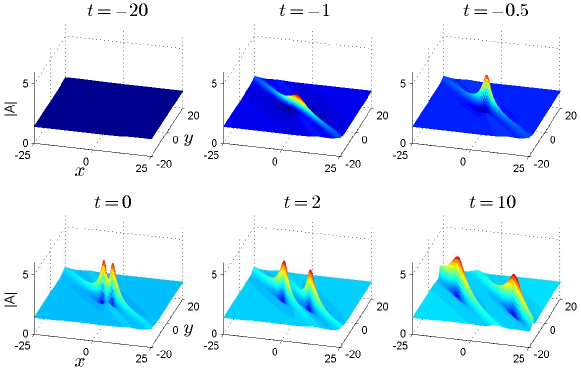
Figure 4: A second-order rogue wave solution (3.21) with $\alpha=1$.

It is noted that when $p^{2}=i$, i.e., $p=\pm e^{i\pi/4}$, the second-order solution (3.19) would approach the constant background when $t\to+\infty$ but approach two lumps which move away from each other when $t\to-\infty$. In other words, this solution describes a process which is opposite of that when $p^{2}=-i$ (see Fig. 4).

III.4 Exploding rogue waves

A third but important subclass of non-fundamental rogue waves is the exploding rogue waves. These rogue waves, which arise from the constant background, can blow up to infinity in finite time at isolated spatial locations. These exploding rogue waves can be obtained from the higher-order rogue waves or multi-rogue waves under certain parameter conditions, as we will demonstrate below.

First, we consider the second-order rogue waves (3.21). When $\alpha=0$, this solution becomes

$$A(x,y,t)=\sqrt{2}\left[1-\frac{(x+y)^{2}+8t-2i(x^{2}-y^{2})}{\Big{(}\frac{1}{2}(x+y)^{2}-4t\Big{)}^{2}+x^{2}+y^{2}}\right].$$ (3.22)

This solution uniformly approaches the constant background $\sqrt{2}$ as $t\to\pm\infty$. But in the intermediate time $t=0$, it blows up to infinity at the origin $(x,y)=(0,0)$. To see this, we notice that at $(x,y)=(0,0)$,

$$A(0,0,t)=\sqrt{2}\hskip 1.13791pt\Big{(}1-\frac{1}{2t}\Big{)},$$ (3.23)

thus this $A$ solution blows up to infinity when $t$ approaches zero (the solution $Q$ blows up to infinity at this time as well). The rate of blowup is $(t-t_{*})^{-1}$, where $t_{*}=0$ is the time of singularity. This exploding process is displayed in Fig. 5. The existence of exploding rogue waves in the DSII equation is a remarkable phenomenon, and their occurrence would be catastrophic in physical systems.

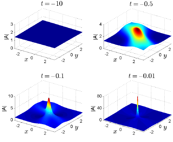
Figure 5: An exploding second-order rogue wave (3.22).

In addition to higher-order rogue waves, multi-rogue waves can also explode under suitable choices of parameters. To demonstrate, we consider the two-rogue-wave solutions whose simplified expressions are given in Eq. (3.14). Taking parameter values

$$p_{1}=1,\quad p_{2}=i,\quad\hat{c}_{11}=\hat{c}_{21}=0,$$ (3.24)

this two-rogue wave becomes

$$A(x,y,t)=\sqrt{2}\ \frac{\tau_{1}}{\tau_{0}},\qquad Q=-1-(2\log\tau_{0})_{xx},$$ (3.25)

where

$$\tau_{0}=x^{2}y^{2}+\left(4t^{2}+\frac{1}{4}\right)(x^{2}+y^{2})+\left(4t^{2}-\frac{3}{4}\right)^{2},$$

$$\tau_{1}=x^{2}y^{2}+\left(4t^{2}-\frac{3}{4}\right)\left(x^{2}+y^{2}+4t^{2}+\frac{5}{4}\right)-4it(x^{2}-y^{2}).$$

At the origin $(x,y)=(0,0)$,

$$A(0,0,t)=\sqrt{2}\ \frac{t^{2}+\frac{5}{16}}{t^{2}-\frac{3}{16}},$$ (3.26)

thus this wave explodes to infinity at times $t_{*}=\pm\sqrt{3}/4$. Its exploding rate is also $(t-t_{*})^{-1}$, where $t_{*}$ is the time of wave singularity. This exploding two-rogue-wave solution is displayed in Fig. 6.

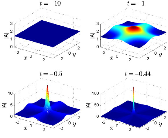
Figure 6: An exploding two-rogue wave (3.25).

It is noted that for the Davey-Stewartson equations, self-similar collapsing solutions have been derived in Nakamura_1982 ; Nakamura_1983 . For the non-integrable Benney-Roskes-Davey-Stewartson equations, wave collapse has also been reported Ablowitz_Segur_1979 ; Ablowitz_collapse2 . Those collapsing solutions are different from our exploding rogue waves since the boundary conditions of those solutions are different. Specifically, those collapsing solutions do not arise from the constant background and are thus not rogue waves.

In this section, only a few subclasses of rogue-wave solutions were examined. The rational solutions in Theorem 1, under parameter conditions (3.1), also contain a lot of other subclasses of rogue waves which are not elaborated in this article. We also note that different choices of parameters can yield the same solutions. For instance, if we take

$$N=1,\quad n_{1}=m_{1}=1,\quad|p_{1}|=|q_{1}|=1$$

in Theorem 1, the resulting solution (2.4) would be equivalent to the two-rogue-wave solution (3.8) with parameters

$$N=2,\quad n_{1}=n_{2}=1,\quad m_{1}=m_{2}=0,\quad|p_{1}|=|p_{2}|=1$$

(see also Eq. (3.14)).

IV Summary and discussions

In this article, we have derived general rogue waves in the Davey-Stewartson-II equation. We have shown that the fundamental rogue waves are line rogue waves which arise from the constant background in a line profile and then retreat back to the constant background again. We have also shown that multi-rogue waves describe the interaction between several fundamental rogue waves, and higher-order rogue waves exhibit different dynamics (such as rising from the constant background but not retreating back to it). In addition, we have discovered exploding rogue waves, which arise from the constant background but blow up to infinity in finite time at isolated spatial points.

It is helpful to compare these rogue waves in the Davey-Stewartson-II equation with those in the Davey-Stewartson-I equation (see OY_DSI ). The biggest difference is that exploding rogue waves exist in the Davey-Stewartson-II equation, but such waves cannot be found in the Davey-Stewartson-I equation OY_DSI . In Appendix C, nonsingularity of rogue waves in the Davey-Stewartson-I equation is analytically proved for a subclass of parameter values, and we conjecture that all rogue waves (which arise from the constant background) are nonsingular in the Davey-Stewartson-I equation.

Other differences on rogue waves also exist between the Davey-Stewartson-I and Davey-Stewartson-II equations. For instance, in the Davey-Stewartson-I equation, fundamental (line) rogue waves can only be oriented along a half of all possible angles in the $(x,y)$ plane OY_DSI ; but in the Davey-Stewartson-II equation, fundamental rogue waves can be oriented along any angle (except diagonal and anti-diagonal angles). This difference has important implications for multi-rogue-wave patterns. For instance, in the Davey-Stewartson-II equation, cross rogue-wave patterns formed by two orthogonally-oriented fundamental rogue waves exist (see Fig. 2); but in the Davey-Stewartson-I equation, cross patterns of multi-rogue waves cannot exist.

Appendix A

In this appendix, we derive the rational solutions to the DSII equation in Theorem 1.

The bilinear form (2.3) of the DSII equation can be derived from

$$\begin{array}[]{l}(D_{x_{1}}D_{x_{-1}}-2)\tau_{n}\cdot\tau_{n}=-2\tau_{n+1}\tau_{n-1},\\[5.0pt] (D_{x_{1}}^{2}-D_{x_{2}})\tau_{n+1}\cdot\tau_{n}=0,\\[5.0pt] (D_{x_{-1}}^{2}+D_{x_{-2}})\tau_{n+1}\cdot\tau_{n}=0,\end{array}$$ (A.1)

by taking the independent and dependent variables as

$$x_{1}=\frac{1}{2}(x+iy),\quad x_{-1}=\frac{\epsilon}{2}(x-iy),\quad x_{2}=\frac{1}{2i}t,\quad x_{-2}=-\frac{1}{2i}t,$$ (A.2)

$$f=\tau_{0},\quad g=\tau_{1},$$ (A.3)

and imposing the complex conjugate condition

$$\overline{\tau_{n}}=\tau_{-n}.$$ (A.4)

The variable transformation (A.2) means that

$$x_{-1}=\epsilon\overline{x_{1}},\quad x_{-2}=\overline{x_{2}}.$$ (A.5)

We first consider the rational solutions for the system (A.1), and then obtain those for (2.3) by imposing the complex conjugate condition (A.4).

It is known that the bilinear equation (A.1) admits determinant solutions

$$\tau_{n}=\det_{1\leq i,j\leq K}\left(m_{ij}^{(n)}\right),$$ (A.6)

where $K$ is a positive integer, $m_{ij}^{(n)}$ is an arbitrary function satisfying the differential and difference relations,

$$\begin{array}[]{l}\partial_{x_{1}}m_{ij}^{(n)}=\varphi_{i}^{(n)}\psi_{j}^{(n)},\\[5.0pt] \partial_{x_{2}}m_{ij}^{(n)}=\varphi_{i}^{(n+1)}\psi_{j}^{(n)}+\varphi_{i}^{(n)}\psi_{j}^{(n-1)},\\[5.0pt] \partial_{x_{-1}}m_{ij}^{(n)}=-\varphi_{i}^{(n-1)}\psi_{j}^{(n+1)},\\[5.0pt] \partial_{x_{-2}}m_{ij}^{(n)}=-\varphi_{i}^{(n-2)}\psi_{j}^{(n+1)}-\varphi_{i}^{(n-1)}\psi_{j}^{(n+2)},\\[5.0pt] m_{ij}^{(n+1)}=m_{ij}^{(n)}+\varphi_{i}^{(n)}\psi_{j}^{(n+1)},\end{array}$$ (A.7)

and $\varphi_{i}^{(n)}$, $\psi_{j}^{(n)}$ are arbitrary functions satisfying

$$\partial_{x_{\nu}}\varphi_{i}^{(n)}=\varphi_{i}^{(n+\nu)},\quad\partial_{x_{\nu}}\psi_{j}^{(n)}=-\psi_{j}^{(n-\nu)},\quad(\nu=\pm 1,\pm 2).$$ (A.8)

The rational solutions are obtained by taking

$$m_{ij}^{(n)}=A_{i}B_{j}\frac{1}{p_{i}+q_{j}}\Big{(}-\frac{p_{i}}{q_{j}}\Big{)}^{n}e^{\xi_{i}+\eta_{j}},$$ (A.9)

$$\varphi_{i}^{(n)}=A_{i}p_{i}^{n}e^{\xi_{i}},\quad\psi_{j}^{(n)}=B_{j}(-q_{j})^{-n}e^{\eta_{j}},$$ (A.10)

$$\xi_{i}=\frac{1}{p_{i}^{2}}x_{-2}+\frac{1}{p_{i}}x_{-1}+p_{i}x_{1}+p_{i}^{2}x_{2},$$ (A.11)

$$\eta_{j}=-\frac{1}{q_{j}^{2}}x_{-2}+\frac{1}{q_{j}}x_{-1}+q_{j}x_{1}-q_{j}^{2}x_{2},$$ (A.12)

where $p_{i}$ and $q_{j}$ are complex constants, $A_{i}$ and $B_{j}$ are differential operators of order $n_{i}$ and $m_{j}$ with respect to $p_{i}$ and $q_{j}$ respectively, defined as

$$A_{i}=\sum_{k=0}^{n_{i}}c_{ik}(p_{i}\partial_{p_{i}})^{n_{i}-k},\quad B_{j}=\sum_{l=0}^{m_{j}}d_{jl}(q_{j}\partial_{q_{j}})^{m_{j}-l},$$ (A.13)

$c_{ik}$, $d_{jl}$ are complex constants, and $n_{i}$, $m_{j}$ are non-negative integers. It is easy to see that the above $m_{ij}^{(n)}$, $\varphi_{i}^{(n)}$ and $\psi_{j}^{(n)}$ satisfy the differential and difference relations (A.7) and (A.8).

Next we impose the complex conjugate condition (A.4) with the restriction (A.5). For this purpose, we consider general rational solutions (A.6) with $2N\times 2N$ determinants (i.e., $K=2N$),

$$\tau_{n}=\det_{1\leq i,j\leq 2N}\left(m_{ij}^{(n)}\right),$$ (A.14)

together with (A.9) and (A.13). In this solution, we impose the parameter conditions

$$p_{N+i}=\frac{\epsilon}{\bar{p}_{i}},\quad q_{N+j}=\frac{\epsilon}{\bar{q}_{j}},\quad n_{N+i}=n_{i},\quad m_{N+j}=m_{j},$$

$$c_{N+i,k}=\sum_{\mu=0}^{k}(-1)^{\mu}{n_{i}-\mu\choose k-\mu}\bar{c}_{i\mu},\quad d_{N+j,l}=\sum_{\nu=0}^{l}(-1)^{\nu}{m_{j}-\nu\choose l-\nu}\bar{d}_{j\nu},$$

for $1\leq i,j\leq N$. Under these parameter conditions, we have

$$\xi_{N+i}=\bar{\xi}_{i},\quad\eta_{N+j}=\bar{\eta}_{j},$$

$$A_{N+i}=\sum_{k=0}^{n_{i}}c_{N+i,k}(-\bar{p}_{i}\partial_{\bar{p}_{i}})^{n_{i}-k}=(-1)^{n_{i}}\sum_{\mu=0}^{n_{i}}\bar{c}_{i\mu}(\bar{p}_{i}\partial_{\bar{p}_{i}}-1)^{n_{i}-\mu},$$

$$B_{N+j}=\sum_{l=0}^{m_{j}}d_{N+j,l}(-\bar{q}_{j}\partial_{\bar{q}_{j}})^{m_{j}-l}=(-1)^{m_{j}}\sum_{\nu=0}^{m_{j}}\bar{d}_{j\nu}(\bar{q}_{j}\partial_{\bar{q}_{j}}-1)^{m_{j}-\nu}.$$

Using the operator identities

$$(\bar{p}_{j}\partial_{\bar{p}_{j}}-1)^{k}\bar{p}_{j}=\bar{p}_{j}(\bar{p}_{j}\partial_{\bar{p}_{j}})^{k},\qquad(\bar{q}_{j}\partial_{\bar{q}_{j}}-1)^{k}\bar{q}_{j}=\bar{q}_{j}(\bar{q}_{j}\partial_{\bar{q}_{j}})^{k},$$

the elements of the determinant in $\tau_{n}$ become

$$m_{i,N+j}^{(n)}=A_{i}B_{N+j}\frac{\bar{q}_{j}}{p_{i}\bar{q}_{j}+\epsilon}(-\epsilon p_{i}\bar{q}_{j})^{n}e^{\xi_{i}+\bar{\eta}_{j}}=(-1)^{m_{j}}\bar{q}_{j}A_{i}\bar{B}_{j}\frac{1}{p_{i}\bar{q}_{j}+\epsilon}(-\epsilon p_{i}\bar{q}_{j})^{n}e^{\xi_{i}+\bar{\eta}_{j}},$$

$$m_{N+i,j}^{(n)}=A_{N+i}B_{j}\frac{\bar{p}_{i}}{\bar{p}_{i}q_{j}+\epsilon}(-\epsilon\bar{p}_{i}q_{j})^{-n}e^{\bar{\xi}_{i}+\eta_{j}}=(-1)^{n_{i}}\bar{p}_{i}\bar{A}_{i}B_{j}\frac{1}{\bar{p}_{i}q_{j}+\epsilon}(-\epsilon\bar{p}_{i}q_{j})^{-n}e^{\bar{\xi}_{i}+\eta_{j}},$$

$$m_{N+i,N+j}^{(n)}=A_{N+i}B_{N+j}\frac{\epsilon\bar{p}_{i}\bar{q}_{j}}{\bar{p}_{i}+\bar{q}_{j}}\Big{(}-\frac{\bar{p}_{i}}{\bar{q}_{j}}\Big{)}^{-n}e^{\bar{\xi}_{i}+\bar{\eta}_{j}}$$

$$=(-1)^{n_{i}+m_{j}}\epsilon\bar{p}_{i}\bar{q}_{j}\bar{A}_{i}\bar{B}_{j}\frac{1}{\bar{p}_{i}+\bar{q}_{j}}\Big{(}-\frac{\bar{p}_{i}}{\bar{q}_{j}}\Big{)}^{-n}e^{\bar{\xi}_{i}+\bar{\eta}_{j}}.$$

Since the $\tau_{n}$ solution can be scaled by an arbitrary constant, we define a scaled $\tau_{n}$ function as

$$\tau_{n}/\prod_{i=1}^{N}(-1)^{n_{i}+m_{i}}\epsilon\bar{p}_{i}\bar{q}_{i}\to\tau_{n}.$$

This scaled $\tau_{n}$ solution can be written as

$$\tau_{n}=\left|\begin{matrix}m_{ij}^{(n)}&\displaystyle\frac{(-1)^{m_{j}}}{\bar{q}_{j}}m_{i,N+j}^{(n)}\cr\vskip 5.0pt\cr\displaystyle\frac{(-1)^{n_{i}}}{\epsilon\bar{p}_{i}}m_{N+i,j}^{(n)}&\displaystyle\frac{(-1)^{n_{i}+m_{j}}}{\epsilon\bar{p}_{i}\bar{q}_{j}}m_{N+i,N+j}^{(n)}\end{matrix}\right|=\left|\begin{matrix}m_{ij}^{(n)}&\widehat{m}_{ij}^{(n)}\cr\vskip 5.0pt\cr\displaystyle\epsilon\overline{\widehat{m}_{ij}^{(-n)}}&\displaystyle\overline{m_{ij}^{(-n)}}\end{matrix}\right|,$$ (A.15)

where

$$\widehat{m}_{ij}^{(n)}\equiv\displaystyle{\frac{(-1)^{m_{j}}}{\bar{q}_{j}}m_{i,N+j}^{(n)}}=A_{i}\bar{B}_{j}\frac{1}{p_{i}\bar{q}_{j}+\epsilon}(-\epsilon p_{i}\bar{q}_{j})^{n}e^{\xi_{i}+\bar{\eta}_{j}}.$$ (A.16)

We can see from (A.15) that this $\tau_{n}$ satisfies the complex conjugate condition (A.4), and thus it satisfies the bilinear equation (2.3) of the DSII equation.

Finally we simplify the above $\tau_{n}$ solution. Using the operator identities

$$(p_{i}\partial_{p_{i}})p_{i}^{n}e^{\xi_{i}}=p_{i}^{n}e^{\xi_{i}}(p_{i}\partial_{p_{i}}+\xi^{\prime}_{i}+n),$$

$$(q_{j}\partial_{q_{j}})(-q_{j})^{-n}e^{\eta_{j}}=(-q_{j})^{-n}e^{\eta_{j}}(q_{j}\partial_{q_{j}}+\eta^{\prime}_{j}-n),$$

where

$$\xi_{i}^{\prime}=-\frac{2}{p_{i}^{2}}x_{-2}-\frac{1}{p_{i}}x_{-1}+p_{i}x_{1}+2p_{i}^{2}x_{2},\quad\eta_{j}^{\prime}=\frac{2}{q_{j}^{2}}x_{-2}-\frac{1}{q_{j}}x_{-1}+q_{j}x_{1}-2q_{j}^{2}x_{2},$$

the rational solutions to the DSII equation can be obtained from (A.13), (A.15) and (A.16) as

$$\tau_{n}=\left|\begin{matrix}m_{ij}^{(n)}&\widehat{m}_{ij}^{(n)}\cr\vskip 5.0pt\cr\displaystyle\epsilon\overline{\widehat{m}_{ij}^{(-n)}}&\displaystyle\overline{m_{ij}^{(-n)}}\end{matrix}\right|,$$ (A.17)

where

$$m_{ij}^{(n)}=(-\frac{p_{i}}{q_{j}})^{n}e^{\xi_{i}+\eta_{j}}\sum_{k=0}^{n_{i}}c_{ik}(p_{i}\partial_{p_{i}}+\xi^{\prime}_{i}+n)^{n_{i}-k}\sum_{l=0}^{m_{j}}d_{jl}(q_{j}\partial_{q_{j}}+\eta^{\prime}_{j}-n)^{m_{j}-l}\frac{1}{p_{i}+q_{j}},$$

$$\widehat{m}_{ij}^{(n)}=(-\epsilon p_{i}\bar{q}_{j})^{n}e^{\xi_{i}+\bar{\eta}_{j}}\sum_{k=0}^{n_{i}}c_{ik}(p_{i}\partial_{p_{i}}+\xi^{\prime}_{i}+n)^{n_{i}-k}\sum_{l=0}^{m_{j}}\bar{d}_{jl}(\bar{q}_{j}\partial_{\bar{q}_{j}}+\overline{\eta^{\prime}_{j}}+n)^{m_{j}-l}\frac{1}{p_{i}\bar{q}_{j}+\epsilon}.$$

Then using the gauge invariance of $\tau_{n}$, we see that $\tau_{n}$ with matrix elements

$$m_{ij}^{(n)}=\sum_{k=0}^{n_{i}}c_{ik}(p_{i}\partial_{p_{i}}+\xi^{\prime}_{i}+n)^{n_{i}-k}\sum_{l=0}^{m_{j}}d_{jl}(q_{j}\partial_{q_{j}}+\eta^{\prime}_{j}-n)^{m_{j}-l}\frac{1}{p_{i}+q_{j}},$$

$$\widehat{m}_{ij}^{(n)}=\sum_{k=0}^{n_{i}}c_{ik}(p_{i}\partial_{p_{i}}+\xi^{\prime}_{i}+n)^{n_{i}-k}\sum_{l=0}^{m_{j}}\bar{d}_{jl}(\bar{q}_{j}\partial_{\bar{q}_{j}}+\overline{\eta^{\prime}_{j}}+n)^{m_{j}-l}\frac{1}{p_{i}\bar{q}_{j}+\epsilon},$$

also satisfies the bilinear equation (A.1) as well as the complex conjugate condition (A.4), thus it satisfies the bilinear equation (2.3) of the DSII equation. This completes the proof of Theorem 1.

Appendix B

In this appendix, we prove that $f$ in Theorem 1 is non-negative for $\epsilon=-1$. In view of Eqs. (2.4) and (2.5), it suffices to show the following lemma.

Lemma 1.  For any $N\times N$ matrices $A$ and $B$, the following $2N\times 2N$ determinant is non-negative:

$$\left|\begin{matrix}A&B\cr-\bar{B}&\bar{A}\end{matrix}\right|\geq 0.$$

Proof.  We will prove this lemma by induction. For $N=1$ the statement in the lemma is obviously true. Let us denote $N\times M$ matrices as

$$A_{NM}=\mathop{\rm mat}_{1\leq i\leq N,\,1\leq j\leq M}\Big{(}a_{ij}\Big{)},\quad B_{NM}=\mathop{\rm mat}_{1\leq i\leq N,\,1\leq j\leq M}\Big{(}b_{ij}\Big{)},$$

where $a_{ij}$ and $b_{ij}$ are complex numbers. Then by the Jacobi formula for determinants, we have

$$\left|\begin{matrix}A_{N+1,N+1}&B_{N+1,N+1}\cr\vskip 5.0pt\cr-\overline{B_{N+1,N+1}}&\overline{A_{N+1,N+1}}\end{matrix}\right|\left|\begin{matrix}A_{NN}&B_{NN}\cr\vskip 5.0pt\cr-\overline{B_{NN}}&\overline{A_{NN}}\end{matrix}\right|$$ (A.18)

$$=\left|\begin{matrix}A_{N+1,N+1}&B_{N+1,N}\cr\vskip 5.0pt\cr-\overline{B_{N,N+1}}&\overline{A_{NN}}\end{matrix}\right|\left|\begin{matrix}A_{NN}&B_{N,N+1}\cr\vskip 5.0pt\cr-\overline{B_{N+1,N}}&\overline{A_{N+1,N+1}}\end{matrix}\right|$$ (A.19)

$$\quad-\left|\begin{matrix}A_{N+1,N}&B_{N+1,N+1}\cr\vskip 5.0pt\cr-\overline{B_{NN}}&\overline{A_{N,N+1}}\end{matrix}\right|\left|\begin{matrix}A_{N,N+1}&B_{NN}\cr\vskip 5.0pt\cr-\overline{B_{N+1,N+1}}&\overline{A_{N+1,N}}\end{matrix}\right|.$$ (A.20)

The right-hand side of this equation can be rewritten as

$$\left|\begin{matrix}A_{N+1,N+1}&B_{N+1,N}\cr\vskip 5.0pt\cr-\overline{B_{N,N+1}}&\overline{A_{NN}}\end{matrix}\right|^{2}+\left|\begin{matrix}A_{N+1,N}&B_{N+1,N+1}\cr\vskip 5.0pt\cr-\overline{B_{NN}}&\overline{A_{N,N+1}}\end{matrix}\right|^{2},$$

which is non-negative. Denoting

$$D_{N}=\left|\begin{matrix}A_{NN}&B_{NN}\cr\vskip 5.0pt\cr-\overline{B_{NN}}&\overline{A_{NN}}\end{matrix}\right|,$$

then Eq. (A.18) gives $D_{N+1}D_{N}\geq 0$. Therefore if $D_{N}>0$, we get $D_{N+1}\geq 0$. If $D_{N}=0$, then by an infinitesimal deformation (for example, $A_{NN}\to A_{NN}+\alpha I_{N}$ with an infinitesimal real number $\alpha$ and the $N\times N$ unit matrix $I_{N}$), the deformed $D_{N}$ becomes positive. Thus the infinitesimally deformed $D_{N+1}$ is non-negative, and so is $D_{N+1}$. This completes the induction and Lemma 1 is proved.

Appendix C

In this appendix, we comment on the nonsingularity of rational solutions for the DSI equation given in OY_DSI . The solution in Theorem 1 of OY_DSI is nonsingular if the real parts of wave numbers $p_{i}$ ($1\leq i\leq N$) are all positive. Because if ${\rm Re}\,p_{i}>0$, then from the appendix in OY_DSI , it is easy to see that the denominator $f$ is given by the determinant of a Hermite matrix whose element can be written as an integral,

$$f=\det_{1\leq i,j\leq N}\Big{(}m_{ij}^{(0)}\Big{)},\quad m_{ij}^{(0)}=\int_{-\infty}^{x_{1}}A_{i}\bar{A}_{j}e^{\xi_{i}+\bar{\xi}_{j}}\,dx_{1}.$$

Here the condition of ${\rm Re}\,p_{i}>0$ (for all $1\leq i\leq N$) is used to guarantee that the antiderivative of $e^{\xi_{i}+\bar{\xi}_{j}}$ (with respect to $x_{1}$) vanishes at $x_{1}=-\infty$. Then for any non-zero vector $\mbox{\boldmath$v$}=(v_{1},v_{2},\cdots,v_{N})$ and ${}^{t}\bar{\mbox{\boldmath$v$}}$ being its complex transpose, we have

$$\mbox{\boldmath$v$}\Big{(}m_{ij}^{(0)}\Big{)}_{i,j=1}^{N}{}^{t}\bar{\mbox{\boldmath$v$}}=\int_{-\infty}^{x_{1}}\Big{|}\sum_{i=1}^{N}v_{i}A_{i}e^{\xi_{i}}\Big{|}^{2}\,dx_{1}>0.$$

This shows that the Hermite matrix $\Big{(}m_{ij}^{(0)}\Big{)}$ is positive definite, hence its determinant $f$ is positive, i.e., $f>0$.

When the real parts of wave numbers $p_{i}$ ($1\leq i\leq N$) are all negative, by slightly modifying the above argument, we can show that the rational solutions in the DSI equation are nonsingular as well.

We conjecture that the rational solutions in the DSI equation, as given in OY_DSI , are actually nonsingular for all wave numbers $p_{i}$ ($1\leq i\leq N$).

References

References

- (1) C. Kharif, E. Pelinovsky and A. Slunyaev, Rogue waves in the ocean (Springer, Berlin, 2009).
- (2) D. R. Solli, C. Ropers, P. Koonath and B. Jalali, “Optical rogue waves”, Nature 450, 1054–1057 (2007).
- (3) D. H. Peregrine, “Water waves, nonlinear Schrödinger equations and their solutions,” J. Australian Math. Soc. B, 25, 16-43 (1983).
- (4) N. Akhmediev, A. Ankiewicz, and J. M. Soto-Crespo, “Rogue Waves and Rational Solutions of the Nonlinear Schr dinger Equation,” Phys. Rev. E 80, 026601 (2009).
- (5) P. Dubard, P. Gaillard, C. Klein, V.B. Matveev, “On multi-rogue wave solutions of the NLS equation and positon solutions of the KdV equation”, Eur. Phys. J. Special Topics 185, 247-258 (2010).
- (6) P. Dubard, V.B. Matveev, “Multi-rogue waves solutions to the focusing NLS equation and the KP-I equation”, Nat. Hazards. Earth. Syst. Sci. 11, 667–672 (2011).
- (7) P. Gaillard, “Families of quasi-rational solutions of the NLS equation and multi-rogue waves”, J. Phys. A: Math. Theor. 44, 435204 (2011).
- (8) A. Ankiewicz, D.J. Kedziora and N. Akhmediev, “Rogue wave triplets”, Phys. Lett. A, 375, 2782–2785 (2011).
- (9) D.J. Kedziora, A. Ankiewicz, and N. Akhmediev, “Circular rogue wave clusters”, Phys. Rev. E 84, 056611 (2011).
- (10) B. Guo, L. Ling, and Q.P. Liu, “Nonlinear Schrödinger equation: Generalized Darboux transformation and rogue wave solutions”, Phys. Rev. E 85, 026607 (2012).
- (11) Y. Ohta and J. Yang, “General high-order rogue waves and their dynamics in the nonlinear Schrödinger equation”, Proc. Roy. Soc. A. 468, 1716-1740 (2012).
- (12) N. Akhmediev, V.M. Eleonskii, and N.E. Kulagin, “Generation of a periodic sequence of picosecond pulses in an optical fiber: Exact solutions”, Sov. Phys. JETP 89, 1542- 1551. [In Russian.]
- (13) N. Akhmediev, V.M. Eleonskii and N.E. Kulagin, “Exact first-order solutions of the nonlinear Schödinger equation”, Theor. Math. Phys. 72, 809–818 (1988).
- (14) A.R. Its, A.V. Rybin, and M.A. Salle, “Exact Integration of Nonlinear Schrödinger equation”, Theor. Math. Phys. 74, 29- 45 (1988).
- (15) M.J. Ablowitz and B.M Herbst, “On homoclinic structure and numerically induced chaos for the nonlinear Schr6dinger equation”, SIAM J. Appl. Math. 50, 339–351 (1990).
- (16) N. Akhmediev, A. Ankiewicz and M. Taki, “Waves that appear from nowhere and disappear without a trace”, Phys. Lett. A 373, 675–678 (2009).
- (17) M.J. Ablowitz, private communication (2012).
- (18) B. Kibler, J. Fatome, C. Finot, G. Millot, F. Dias, G. Genty, N. Akhmediev, and J.M. Dudley, “The Peregrine soliton in nonlinear fibre optics”, Nature Physics, 6, 790–795 (2010).
- (19) A. Chabchoub, N. Hoffmann, M. Onorato, A. Slunyaev, A. Sergeeva, E. Pelinovsky, and N. Akhmediev, “Observation of a hierarchy of up to fifth-order rogue waves in a water tank”, Phys. Rev. E 86, 056601 (2012).
- (20) A. Ankiewicz, J. M. Soto-Crespo, and N. Akhmediev, “Rogue waves and rational solutions of the Hirota equation”, Phys. Rev. E, 81, 046602 (2010).
- (21) S. Xu, J. He and L. Wang, “The Darboux transformation of the derivative nonlinear Schr dinger equation”, J. Phys. A 44, 305203 (2011).
- (22) B. Guo, L. Ling and Q.P. Liu, “High-order solutions and generalized Darboux transformations of derivative nonlinear Schrödinger equations”, Stud. Appl. Math. DOI: 10.1111/j.1467-9590.2012.00568.x (2012).
- (23) Y. Ohta and J. Yang, “Rogue waves in the Davey-Stewartson I equation,” Phys. Rev. E 86, 036604 (2012).
- (24) D. J. Benney and G. Roskes, “Wave instabilities”, Stud. Appl. Math. 48, 377–385 (1969).
- (25) A. Davey and K. Stewartson, “On three-dimensional packets of surface waves”, Proc. R. Soc. London, A 338, 101–110 (1974).
- (26) M.J. Ablowitz and H. Segur, Solitons and the Inverse Scattering Transform (SIAM, Philadelphia, 1981).
- (27) J. Satsuma and M. J. Ablowitz, “Two-dimensional lumps in nonlinear dispersive systems,” J. Math. Phys. 20, 1496–1503 (1979).
- (28) M.J. Ablowitz and P.A. Clarkson, Solitons, Nonlinear Evolution Equations and Inverse Scattering (Cambridge University Press, Cambridge, 1991).
- (29) M. Tajiri and T. Arai, “Growing-and-decaying mode solution to the Davey-Stewartson equation,” Phys. Rev. E 60, 2297–2305 (1999).
- (30) A. Nakamura, “Explode-decay mode lump solitons of a two-dimensional nonlinear Schrödinger equation”, Phys. Lett. A 88, 55–56 (1982).
- (31) A. Nakamura “Exact explode-decay soliton solutions of a coupled nonlinear Schrödinger equation,” J. Phys. Soc. Jpn. 52, 3713–3721 (1983).
- (32) M.J. Ablowitz and H. Segur, “On the evolution of packets of water waves,” J. Fluid Mech. 92, 691–715 (1979).
- (33) M.J. Ablowitz, I. Bakirtas, and B. Ilan, “Wave collapse in a class of nonlocal nonlinear Schrödinger equations,” Physica D 207, 230–253 (2005).