What controls the magnetic geometry of M dwarfs?

Abstract

Context. Observations of rapidly rotating M dwarfs show a broad variety of large-scale magnetic fields encompassing dipole-dominated and multipolar geometries. In dynamo models, the relative importance of inertia in the force balance – quantified by the local Rossby number – is known to have a strong impact on the magnetic field geometry.

Aims. We aim to assess the relevance of the local Rossby number in controlling the large-scale magnetic field geometry of M dwarfs.

Methods. We explore the similarities between anelastic dynamo models in spherical shells and observations of active M-dwarfs, focusing on field geometries derived from spectropolarimetric studies. To do so, we construct observation-based quantities aimed to reflect the diagnostic parameters employed in numerical models.

Results. The transition between dipole-dominated and multipolar large-scale fields in early to mid M dwarfs is tentatively attributed to a Rossby number threshold. We interpret late M dwarfs magnetism to result from a dynamo bistability occurring at low Rossby number. By analogy with numerical models, we expect different amplitudes of differential rotation on the two dynamo branches.

1 Introduction

M dwarfs – the lowest-mass stars of the main sequence – are of prime interest to study stellar dynamos operating in physical conditions quite remote from the solar case. During the past few years, their surface magnetic fields have been investigated using two complementary approaches (for recent reviews see Donati & Landstreet 2009; Reiners 2012). On the one hand, with spectroscopy in unpolarized light (i.e. measuring the Stokes parameter I) the average magnetic field strengths (hereafter referred to as $\left\langle\rm B_{\rm I}\right\rangle$) of tens of stars spanning the whole M-dwarf spectral class have been derived. From such measurements Reiners & Basri (2007) have concluded that no significant change in $\left\langle\rm B_{\rm I}\right\rangle$ occurs when stars become fully convective (spectral type M3/M4) and Reiners et al. (2009) could constrain the rotation-magnetic field relation ($\left\langle\rm B_{\rm I}\right\rangle$ increases towards short rotation periods until it reaches a plateau at $\sim 3\leavevmode\nobreak\ \hbox{$\rm kG$}$). On the other hand, the measurement of circular polarization (Stokes V) in spectral lines of M dwarfs provides a constraint on the orientation and polarity of the field at large and intermediate scales. Modelling of the surface field performed with Zeeman-Doppler imaging (ZDI, Semel 1989) on a sample of about 20 M0-M8 dwarfs points towards a broad variety of magnetic field geometries. Partly-convective stars as well as a few fully-convective ones feature complex magnetic structures (e.g. Donati et al. 2008; Morin et al. 2010) while most fully-convective ones host a strong axial dipole component Morin et al. (2008a, b).

Explaining such a diversity in the magnetic field geometry is one of the main goals of stellar dynamo theory. However, as the numerical simulations cannot directly access the parameter regime where such dynamos are thought to operate, asymptotic scaling laws are of prime interest to check the relevance of the dynamo models (Christensen 2010). Scaling laws derived from geodynamo-like models (i.e. incompressible flow and no-slip boundaries) successfully fit the magnetic field strength of a broad range of astrophysical objects, encompassing Earth, Jupiter and some rapidly-rotating M dwarfs (Christensen et al. 2009). Such similarities between the dynamos in planets and rapidly-rotating stars motivate the comparison of some planetary dynamo results with observations of active M dwarfs.

In geodynamo models, the relative contribution of inertia and Coriolis force in the global balance is known to have a strong impact on the magnetic field geometry (e.g. Sreenivasan & Jones 2006). Christensen & Aubert (2006) suggest that the ratio of these two forces can be quantified by the so-called “local Rossby number” defined by $\text{Ro}_{l}=u_{\text{rms}}/\Omega l$, $l$ being the typical flow lengthscale. This dimensionless parameter has been found to be a rather universal quantity that allows to separate dipolar and multipolar dynamo models: a sharp transition between these two types of dynamo occurs around $\text{Ro}_{l}\simeq 0.1$. However, this has been recently challenged by some models that employed stress-free mechanical boundary conditions, more appropriate when modelling stellar dynamos (e.g. Goudard & Dormy 2008). Simitev & Busse (2009) for instance found that a dipolar and a multipolar magnetic field can coexist at the same parameter regime depending on the initial condition. This magnetic bistability phenomenon can lead to multipolar solutions even for $\text{Ro}_{l}<0.1$ (Schrinner et al. 2012).

In addition, most of these studies have been conducted under the Boussinesq approximation that assumes the reference state to be constant with radius. While this assumption is suitable for modelling the geodynamo, it becomes questionable in the stellar interiors, where density increases by several orders of magnitude. Anelastic and compressible dynamo models indeed indicate a strong influence of the density contrast on the geometry of the magnetic field: some weakly stratified simulations of Dobler et al. (2006) are dipole-dominated, while the strongly stratified models of Browning (2008) are multipolar. The parameter study of Gastine et al. (2012) extends the bistability phenomenon to a broader parameter range and confirms that strongly stratified models tend to produce multipolar dynamos.

Following the conclusions by Schrinner et al. (2012) and Gastine et al. (2012) (hereafter GDW12), the main aim of this letter is to compare the results of the later study with spectropolarimetric observations of M dwarfs.

2 The dynamo model

We consider MHD simulations of a conducting anelastic fluid in spherical shells rotating at a constant rotation rate $\Omega$ about the $z$-axis. Following Gilman & Glatzmaier (1981), the governing MHD equations are non-dimensionalised using the shell thickness $d=r_{o}-r_{i}$ as the reference lengthscale and $\Omega^{-1}$ as the time unit. Our dynamo model results are then characterised by several dimensionless diagnostic parameters. The rms flow velocity for instance is given by the Rossby number $\text{Ro}=u_{\text{rms}}/\Omega d$. Following Christensen & Aubert (2006), we also employ the aforementioned local Rossby number $\text{Ro}_{l}=\text{Ro}\,\bar{\ell}_{u}/\pi$, that is known to be a more appropriate measure to quantify the impact of inertia on the magnetic field geometry. The mean spherical harmonic degree $\bar{\ell}_{u}$ is obtained from the kinetic energy spectrum and relates to the typical flow lengthscale $l$ through:

$$l=\pi\,d/\bar{\ell}_{u}\quad\text{with}\quad\bar{\ell}_{u}=\sum_{\ell}\ell\dfrac{\langle\@vec{u}_{\ell}\cdot\@vec{u}_{\ell}\rangle}{\langle\@vec{u}\cdot\@vec{u}\rangle},$$ (1)

where $\@vec{u}_{\ell}$ is the flow at a given spherical harmonic degree $\ell$ and the brackets correspond to an average over time and radius.

The magnetic field strength is measured by the Elsasser number $\Lambda=B_{\text{rms}}^{2}/\rho\mu\lambda\Omega$, where $\rho$ is the density, and $\mu$ and $\lambda$ are the magnetic permeability and diffusivity. The geometry of the surface field is quantified by its dipolarity $f_{\text{dip}}=\@vec{B}_{\ell=1,m=0}^{2}(r=r_{o})/\sum_{\ell,m}^{\ell_{\text{max}}}\@vec{B}_{\ell,m}^{2}(r=r_{o})$, the ratio of the magnetic energy of the dipole to the magnetic energy contained in spherical harmonic degrees up to $\ell_{\text{max}}=11$ (see Christensen & Aubert 2006).

The dimensionless MHD equations are advanced in time with the spectral code MagIC (Wicht 2002; Gastine & Wicht 2012) that uses the anelastic formulation of Lantz & Fan (1999) and has been validated against several dynamo benchmarks (Jones et al. 2011). We rely in the following on the results of the parameter study of GDW12. Although these simulations have been initially tailored to model the dynamo of giant planets, the differences in the reference properties (i.e. density and gravity profiles) are not expected to be of prime influence. Similarities between dynamos in planets and low-mass stars are indeed emphasised by geodynamo-based scaling laws (Christensen 2010) and previous Boussinesq models employed in the stellar dynamo context (e.g. Schrinner et al. 2012; Simitev & Busse 2012).

3 Spectropolarimetric observations

Spectropolarimetric observations of 23 active M0-M8 dwarfs with rotation periods ranging from 0.4 to 19 days have been carried out. For each star at least one time-series of unpolarized and circularly polarized spectra sampling a few rotation periods has been obtained. The data reduction and analysis is detailed by Donati et al. (2006, 2008) and Morin et al. (2008a, b, 2010).

The relative importance of inertia with respect to the Coriolis force in the convection zone of these stars is assessed through an empirical Rossby number given by

$$\text{Ro}_{\text{emp}}=\dfrac{\hbox{$P_{\rm rot}$}}{\tau_{\text{conv}}},$$ (2)

where $\tau_{\text{conv}}$ is the empirical turnover timescale of convection based on the rotation-activity relation (Kiraga & Stepien 2007). This Rossby number misses explicitly the flow lengthscale $l$ involved in $\text{Ro}_{l}$. However, as $\tau_{\text{conv}}$ is based on the average convective turnover time it encompasses this scale information to some extent. We thus use $\text{Ro}_{\text{emp}}$ as our best available proxy for $\text{Ro}_{l}$.

For each obtained spectrum, an average line profile with increased signal-to-noise ratio is computed using the least-squares deconvolution technique (LSD, Donati et al. 1997). Each time-series of LSD profiles is modelled with ZDI, resulting in a map of the large-scale component of the surface magnetic field vector that satisfies a maximum-entropy criterion. The large-scale magnetic fields of most of these stars fall into two distinct groups: one is dominated by a strong axial dipolar component and the other by a much weaker and non-axisymmetric field. We could not identify any ZDI reconstruction bias that would spuriously produce such a separation, and exclude an effect of limited resolution as both groups span largely overlapping ranges of $v\sin i$.

Following Morin et al. (2011), we define an Elsasser number based on the averaged unsigned large-scale magnetic field $\left\langle\rm B_{\rm V}\right\rangle$ which roughly characterises the ratio of Lorentz and Coriolis forces. $\eta$ is obtained by rescaling a reference solar magnetic diffusivity of $\eta_{\odot}=10^{11}\leavevmode\nobreak\ {\rm cm}^{2}{\rm s}^{-1}$ (Stix 1989) to the M dwarfs with a MLT argument. We also consider the fraction of the magnetic energy that is recovered in the axial dipole mode in ZDI maps. The spatial resolution of such maps mostly depends on $v\sin i$ and the actual degree and order $\ell_{\text{max}}$ up to which the reconstruction can be performed ranges from 4 to 10, although very little energy is recovered in modes with $4<\ell\leq 10$. We therefore directly compare this quantity to the dipolarity employed in numerical models and term them both $f_{\text{dip}}$. We however note that in simulations, $f_{\text{dip}}$ does not strongly depend on the chosen $\ell_{\text{max}}$, whereas for the observation-based dipolarity, considering the ratio of magnetic energy in the axial dipole relative to the total magnetic energy derived from unpolarized spectroscopy (instead of the large-scale magnetic energy derived from spectropolarimetric data with ZDI) would lead to much lower values of $f_{\text{dip}}$ (cf. Reiners & Basri 2009). We attribute this difference to the low magnetic Reynolds number ($\text{Rm}\sim 100-500$) accessible by numerical simulations which does not allow for a significant small-scale field to be generated – hence the weak dependence of $f_{\text{dip}}$ on $\ell_{\text{max}}$ – while in stellar interiors large-scale and small-scale dynamo action likely coexist (e.g. Cattaneo & Hughes 2009).

4 Results

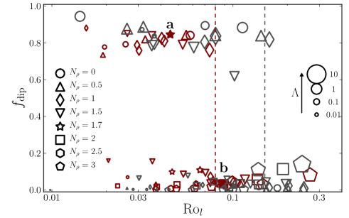
Figure 1: $f_{\text{dip}}$ plotted against $\text{Ro}_{l}$ in anelastic dynamo models. Red (grey) symbols correspond to simulations in thick (thin) shells ($r_{i}/r_{o}=0.2$ and $r_{i}/r_{o}=0.6$, respectively) and their size is scaled according to the value of the surface field, expressed in units of the square root of the Elsasser number. Each type of symbols corresponds to a density contrast. The two closed symbols correspond to two cases further discussed in Fig. 3. The vertical lines mark the tentative limits for dipolar dynamos.

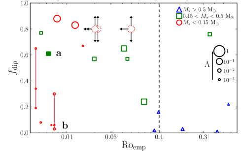
Figure 2: Observational counterpart of Fig. 1. The vertical dashed line marks the tentative limit for the dipolar regime. For the two stars exhibiting the largest temporal variations, the individual epochs are shown and connected by a vertical red line. Dotted red circles with black arrows correspond to stars from Morin et al. (2010) for which a definite ZDI reconstruction could not be achieved, but an upper limit for the rotation period and an estimate of dipolarity were derived. The two closed symbols correspond to two selected stars discussed in Fig. 4.

Figure 1 shows $f_{\text{dip}}$ versus $\text{Ro}_{l}$ in the numerical models, which use the anelastic approximation with density contrasts up to $N_{\rho}=\ln(\rho_{\text{bot}}/\rho_{\text{top}})=3$ and stress-free (or mixed) boundary conditions. Figure 2 displays the relative dipole strength of M stars against $\text{Ro}_{\text{emp}}$ derived from spectropolarimetric observations.

The numerical models cluster in two distinct dynamo branches: the upper branch corresponds to the dipole-dominated regime ($f_{\text{dip}}>0.6$), while the dynamo models belonging to the lower branch have a multipolar magnetic field ($f_{\text{dip}}<0.2$). In agreement with the geodynamo models, the dipolar branch is bounded by a maximum $\text{Ro}_{l}$, beyond which all the models become multipolar (Christensen & Aubert 2006). Although a small dependence on the shell thickness is noticeable, the dipolar branch vanishes around $\text{Ro}_{l}\simeq 0.1$ for both spherical shell geometries considered by GDW12. However, in contrast with most of the previous Boussinesq studies, the multipolar branch also extends well below $\text{Ro}_{l}\simeq 0.1$, where both dipolar and multipolar solutions can coexist (see also Schrinner et al. 2012). In the parameter range covered by our numerical models, bistability of the magnetic field is in fact quite common, meaning that both a dipole-dominated and a multipolar field are possible configurations at the same set of parameters. The type of solution is then selected by the geometry and the amplitude of the initial seed magnetic field (Busse & Simitev 2006; Simitev & Busse 2009). The multipolar branch found at $\text{Ro}_{l}<0.1$ is partly composed by the multipolar component of such bistable dynamos but also encompasses all the stratified models with $N_{\rho}\geq 2$, for which no dipolar solutions are found (GDW12).

The comparison between these results and the observations of stellar magnetic fields suffers from the difficulty to relate the diagnostic parameters of the dynamo models (i.e. $\text{Ro}_{l}$, $\Lambda$ and $f_{\text{dip}}$) to their stellar counterparts. Within these limits, the separation into two dynamo branches seems to be relevant to the sample of active M dwarfs displayed in Fig. 2. In fact, all the early M stars (with $M_{\star}>0.5\,\text{M}_{\odot}$) show multipolar magnetic fields with $f_{\text{dip}}<0.2$; being slow rotators they fall into the $\text{Ro}_{\text{emp}}\geq 0.1$ regime (Reiners & Mohanty 2012). The observations of mid M dwarfs suggest a possible transition between dipole-dominated and multipolar magnetic fields close to $\text{Ro}_{\text{emp}}\sim 0.1$, although CE Boo does not fit into this picture (green square in the upper right corner of Fig. 2). Late M dwarfs (with $M_{\star}<0.15\,\text{M}_{\odot}$) seem to operate in two different dynamo regimes: the first ones show a strong dipolar magnetic field, while others present a weaker multipolar magnetic structure with a significant time variability (emphasised by the vertical red lines in Fig. 2). These important time variations of the dipole strength are also frequently observed in multipolar dynamo models with low $\text{Ro}_{l}$ (e.g. Schrinner et al. 2012, GDW12) but are not visible in Fig. 1, where time-averaged properties are considered. We note that the values of $\tau_{\text{conv}}$ entering Ro${}_{\text{emp}}$ are poorly constrained for M dwarfs. Assuming a stronger (weaker) mass-dependence would mostly expand (shrink) the x-axis of Fig. 2 without changing our conclusions. The uncertainties on $f_{\text{dip}}$ typically lie in the range 0.1-0.3 (see discussion in Morin et al. 2010), which does not question the identification of two distinct branches.

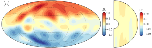
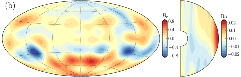
Figure 3: Surface radial magnetic field $B_{r}(r=r_{0})$ and axisymmetric zonal flows $\overline{u_{\phi}}$ for a dipolar dynamo model with $N_{\rho}=1.7$ (a) and a multipolar one with $N_{\rho}=2$ (b). The maps of $B_{r}$ have been low-pass filtered up to $\ell_{\text{max}}=10$. Magnetic fields are expressed in units of the square root of the Elsasser number and velocities in units of the Rossby number.

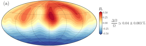
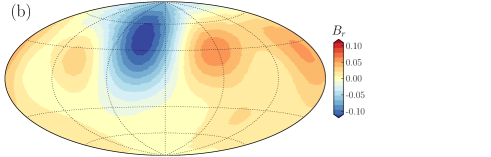
Figure 4: Surface radial magnetic field of V374 Peg (a) and GJ 1245 B (b) recovered with ZDI from spectropolarimetric observations. The field has been reconstructed up to $\ell_{\text{max}}=10$ (4) for V374 Peg (GJ 1245 B). Surface differential rotation of V374 Peg has been derived by Morin et al. (2008b) from spectropolarimetric observations, while this was not possible for GJ 1245 B. Magnetic fields are expressed in units of the square root of the Elsasser number.

The two dynamo branches found in our numerical models also differ by their main force balance, at least in the bistability region (i.e. $\text{Ro}_{l}<0.1$). The dipolar branch encompasses models with Elsasser number around unity that suggest a first-order contribution of the Lorentz force in the main balance (the dynamo then operates under the so-called “magnetostrophic balance”, e.g. Sreenivasan & Jones 2006). In contrast, at low $\text{Ro}_{l}$, the models belonging to the multipolar branch have weaker magnetic fields (see Fig. 1 and Tab. 2 in GDW12), meaning that the Lorentz force may not enter in the first-order balance. In that case, significant geostrophic zonal flows (i.e. aligned on coaxial cylinders) can possibly develop (e.g. Gastine & Wicht 2012). Note that beyond $\text{Ro}_{l}>0.1$, the multipolar dynamos are strong enough to yield a magnetostrophic force balance due to larger Rayleigh numbers. This correspondence between high dipolar fraction and strong large-scale magnetic field is also present in spectropolarimetric observations (Morin et al. 2011). Figure 3 illustrates these two types of dynamos for two typical models with $\text{Ro}_{l}<0.1$. While the upper panel shows a dipole-dominated solution with a very weak differential rotation, the lower one has a multipolar field that goes along with significant zonal flows that become nearly geostrophic close to the equator. These strong zonal winds affect the dynamo mechanism via the $\Omega$-effect, i.e. the production of toroidal field by the shear. This $\Omega$-effect plays only a minor role in the field production of the dipole-dominated models that can be categorised as “$\alpha^{2}$-dynamos”, according to the mean-field description (e.g. Chabrier & Küker 2006). In contrast, dynamos on the multipolar branch can be classified as $\alpha\Omega$ or $\alpha^{2}\Omega$, at least in the low $\text{Ro}_{l}$ regime.

To a certain extent, these differences are also noticeable in the reconstructed fields of M dwarfs as illustrated in Fig. 4. While V374 Peg (upper panel) has a dipole-dominated magnetic field and a very weak differential rotation, GJ 1245 B (lower panel) presents a weaker amplitude multipolar field with important time variability (one of the vertical red lines in Fig. 2). If, as suggested in the present study, the multipolar fields observed in several late M dwarfs are the consequence of a dynamo bistability occurring at low $\text{Ro}_{l}$, the numerical models would then suggest a significant differential rotation in these stars ($\Delta\Omega/\Omega\sim 5\%$ in the Fig. 3b model). However, this cannot be verified from the available data as surface differential rotation has been determined for one star of the sample only (a dipolar one, see Fig. 4a).

5 Conclusion

Spectropolarimetric observations of active M dwarfs and dynamo models show a broad variety of magnetic geometries (see Gastine et al. 2012; Morin et al. 2010, and references therein). In both cases, dipolar and multipolar large-scale magnetic fields are found to coexist at low Rossby numbers. In the present letter we critically discuss the analogy between these two results.

We derive observation-based quantities aimed to reflect the diagnostic parameters employed in the numerical models ($\text{Ro}_{l}$, $\Lambda$ and $f_{\text{dip}}$), although these crude proxies are not expected to provide a direct quantitative match. Within these limits, we draw an interesting analogy between the observational parameters and their numerical counterparts: for large values of the Rossby numbers multipolar fields are found, while below a critical value around $\text{Ro}_{l}\sim\text{Ro}_{\text{emp}}\sim 0.1$, a bistable region exists where both dipolar and multipolar fields can be generated.

Several limitations must be noted though. (i) The spectropolarimetric sample is biased as all stars at high (low) $\text{Ro}_{\text{emp}}$ are partly (fully) convective. Thus it is not yet clear if the change in $f_{\text{dip}}$ observed around $\text{Ro}_{\text{emp}}\sim 0.1$ can be attributed to a threshold in $\text{Ro}_{l}$ or rather to the drastic changes in stellar structure occurring at the fully-convective transition. (ii) As the numerical models of GDW12 do not attempt to model a tachocline, they might miss some important features of early M dwarfs magnetism. However these issues do not question the validity of the agreement between observations and simulations regarding the existence of a bistable dynamo regime at low $\text{Ro}_{l}$ for fully-convective stars. (iii) In numerical models, the dipolar branch only exists for mild density contrasts ($N_{\rho}<2$), much below the stratification of stellar interiors. Different assumptions from those used by GDW12 could possibly extend the dipolar regime towards higher stratifications, for instance by using different values of Prandtl numbers (Simitev & Busse 2009) or radius-dependent properties (e.g. thermal and ohmic diffusivities).

However, the analogy between dynamo simulations and magnetic properties of M dwarfs can be further assessed with more realistic numerical models, and additional observations as it implies that: (i) stars with multipolar fields can be found over the whole parameter range where also dipole-dominated large-scale fields are observed; (ii) in the bistable domain, stars on the multipolar branch have a much stronger surface differential rotation than stars hosting dipole-dominated large-scale fields.