Subdomain geometry of hyperbolic type metrics
Abstract.
Given a domain we study the quasihyperbolic and the distance ratio metrics of and their connection to the corresponding metrics of a subdomain . In each case, distances in the subdomain are always larger than in the original domain. Our goal is to show that, in several cases, one can prove a stronger domain monotonicity statement. We also show that under special hypotheses we have inequalities in the opposite direction.
Key words and phrases:
quasihyperbolic metric, distance ratio metric , Euclidean metric, inequalities2010 Mathematics Subject Classification:
Primary 30F45; Secondary 30C651. Introduction
Recently many authors have studied what we call ”hyperbolic type metrics” of a domain [7, 8, 10, 12, 16, 20]. Some of the examples are the Apollonian metric, the Möbius invariant metric, the quasihyperbolic metric and the distance ratio metric. The term ”hyperbolic type metric” is for us just a descriptive term, we do not define it. The term is justified by the fact that the metric is similar to the hyperbolic metric of the unit ball In this paper we will study a hyperbolic type metric with the following two properties:
-
(1)
if is a subdomain, then for all ,
- (2)
In particular, we require that is defined for every proper subdomain of The purpose of this paper is to study the subdomain monotonicity property (1) and to prove conditions under which we have a quantitative refinement of (1).
For a subdomain and the distance ratio metric is defined by
where denotes the Euclidean distance from to . Sometimes we abbreviate by writing just The above form of the metric, introduced in [22], is obtained by a slight modification of a metric that was studied in [5, 6]. The quasihyperbolic metric of is defined by the quasihyperbolic length minimizing property
where represents the family of all rectifiable paths joining and in , and is the quasihyperbolic length of (cf. [6]). For a given pair of points the infimum is always attained [5], i.e., there always exists a quasihyperbolic geodesic which minimizes the above integral, and furthermore with the property that the distance is additive on the geodesic: for all . If the domain is emphasized we call a -geodesic. In this paper, our main work is to refine some inequalities between metric, metric and the Euclidean metric. Both the distance ratio and the quasihyperbolic metric qualify as hyperbolic type metrics because
-
both are defined for every proper subdomain of
-
for the case of the unit ball both are comparable to the hyperbolic metric of see Section 2 below,
-
it is well-known that both metrics satisfy the above properties (1) and (2).
These metrics have recently been studied, e.g., in [7, 10, 16]. We mainly study the following three problems and our main results will be given in Section 2, Section 3 and Section 4 respectively.
Problem 1.1.
For some special domains, can we obtain certain upper estimates for the quasihyperbolic metric in terms of the distance ratio metric?
Indeed, inequalities of this type were used to characterize so called -domains in [22].
Problem 1.2.
Is there some relation between metric and the Euclidean metric? The same question can be asked for metric and the Euclidean metric?
Let and be proper subdomains of . It is well know that if then for all ,
and
We expect some better results to hold for some special class of domains. This motivates the following question.
Problem 1.3.
Let be two proper subdomains in such that is either or a discrete set. Does there exist a constant such that for all , the following holds:
| (1.4) |
where for
Our main results for Problem 1.1 are Theorems 2.5 and 2.9, for Problem 1.2 Theorems 3.3 and 3.4 and for Problem 1.3 Theorems 4.3 and 4.6. We also formulate some open problems and conjectures. Finally, it should be pointed out that there are many more metrics for which the above problems could be studied. For some of these metrics, see [24].
2. Results concerning Problem 1.1
In this section, we study Problem 1.1 and our mains results are Theorems 2.5 and 2.9. The following proposition, which will be used in the proof of Theorems 2.5, gathers together several basic well-known properties of the metrics and , see for instance [6, 23]. The motivation comes from the well-known inequality
| (2.1) |
for a domain where One can ask: when do both the metrics and (or ) coincide ?
Proposition 2.2.
-
(1)
For , we have
-
(2)
Moreover, for and , we have
-
(3)
Let be a domain and . Let be such that . Then for all , we have
-
(4)
For we have
with equality on the right hand side when
Proof.
The hyperbolic geometry of serves as model for the quasihyperbolic geometry and we will use below a few basic facts of the hyperbolic metric of These facts appear in standard textbooks of hyperbolic geometry and also in [23, Section 2]. For the case of , we make use of an explicit formula [23, (2.18)] to the effect that for
| (2.3) |
It is readily seen that
and it is well-known by [1, Lemma 7.56] that a similar inequality also holds for
Remark 2.4.
The proofs of Proposition 2.2 (1) and (2) show that the diameter of is a geodesic of and hence the quasihyperbolic distance is additive on a diameter. At the same time we see that the metric is additive on a radius of the unit ball but not on the full diameter because for
In order to obtain certain upper estimates for the quasihyperbolic metric, in terms of the distance ratio metric, we present the following theorem.
Theorem 2.5.
-
(1)
For and , we have
-
(2)
Let be a domain, and If and , then we have
Proof.
(1) Fix and the geodesic of the hyperbolic metric joining them. Then and for all we have
Therefore, by Proposition 2.2 (4)
for . The inequality, , follows from (2.1).
This completes the proof of the theorem. ∎
Remark 2.6.
Theorem 2.5 (1) refines the well-known inequality in [21, Lemma 2.11] and [23, Lemma 3.7(2)] for the case of . We have been unable to prove a similar statement for a general domain. However, a similar result for is obtained in the sequel (see Theorem 2.9). To obtain this, we collect some basic properties.
We here introduce a lemma which is a modification of [9, Lemma 4.9].
Lemma 2.8.
Let and with . Then implies .
Proof.
Let . By (2.7) the angle determines the point uniquely up to a rotation about the line through 0 and . By symmetry and similarity it is sufficient to consider only the case and . We will show that the function
is strictly increasing on , where
For , a simple calculation gives
and hence
If , then we see that
and hence is implying the assertion. ∎
Theorem 2.9.
Let . Then
-
(1)
for and with
-
(2)
for , and
where .
Proof.
(1) We may assume that . Fix . Now and by Lemma 2.8 the quantity attains its maximum when is maximal, which is equivalent to . Thus,
and the first inequality follows.
Let us next prove the second inequality. We define the functions and by
Because
for and , we have . Thus
The function is convex, since
Therefore, on and both imply the assertion.
(2) We prove that
where or . We may assume . Now
and is equivalent to or . The assertion follows from (2.7). ∎
Remark 2.10.
-
(1)
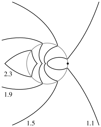
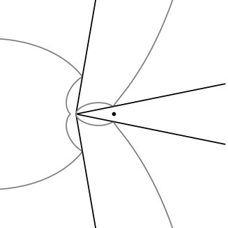
In Theorem 2.9 (1), the constant appears with the bound . This upper bound of is not sharp as can be seen from the proof. By computer simulations, we obtained that the sharp upper bounds are for and for . Lindén [12] proved the limiting case of Theorem 2.9 (1) with the constant For some of the level sets are displayed in Figure 1.
-
(2)
Let be a domain, and let with For given if there exists some constant such that , then by the definition of -metric we have . We also see from [22, Lemma 2.53] that with depending only on .
3. Results concerning Problem 1.2
In this section, our main goal is to study Problem 1.2, that is, to compare the Euclidean metric and the quasihyperbolic metrics defined in a domain. Our main result is Theorem 3.3.
In the next lemma, we recall a sharp inequality for the hyperbolic metric of the unit ball proved in [23, (2.27)].
Lemma 3.1.
For , let be as in . Then
where equality holds for .
Earle and Harris [3] provided several applications of this inequality and extended this inequality to other metrics such as the Carathéodory metric. Notice that Lemma 3.1 gives a sharp bound for the modulus of continuity
For a -quasiconformal homeomorphism
an upper bound for the modulus of continuity is well-known, see [23, Theorem 11.2]. For the result is sharp for each , see [11, p. 65 (3.6)]. The particular case yields a classical Schwarz lemma.
As a preliminary step we record Jung’s Theorem [2, Theorem 11.5.8] which gives a sharp bound for the radius of a Euclidean ball containing a given bounded domain.
Lemma 3.2.
Let be a domain with . Then there exists such that , where .
Theorem 3.3.
-
(1)
If are arbitrary and , then
where the first inequality becomes equality when . Moreover, the identity map has the sharp modulus of continuity .
-
(2)
Let be a domain with and . Then we have
for all distinct with equality in the first step when and . Moreover, the identity map has the sharp modulus of continuity .
Proof.
(1)
Without loss of generality, we assume that
. We divide the proof into two cases.
Case I: The points and are both on a diameter of .
If , by Proposition 2.2(1)
we have
and hence
It is easy to verify that is equivalent to .
If , then the proof goes in a similar way. Indeed, in this situation
is equivalent to
which is trivial as the left hand term is . Equality clearly holds if .
Case II: The points and are arbitrary in .
Choose such that with and on a diameter of . Then
where the first inequality holds trivially and the second holds by Case I. The sharp modulus of continuity can be obtained by a trivial rearrangement of the first inequality from the statement.
A counterpart of Theorem 3.3 for the distance ratio metric can be formulated in the following form (we omit the proofs, since they are very similar to the proofs of Theorem 3.3).
Theorem 3.4.
-
(1)
If are arbitrary and , then
where the first inequality becomes equality when . Moreover, the identity map has the sharp modulus of continuity .
-
(2)
Let be a domain with and . Then we have
for all distinct with equality in the first step when and . Moreover, the identity map has the sharp modulus of continuity .
4. Results concerning Problem 1.3
In this final section we present our results on Problem 1.3.
Theorem 4.1.
Proof.
Obviously, is a discrete set. For each , we prove that
| (4.2) |
Without loss of generality, we may assume that and . Then and Hence,
which proves equation (4.2).
Given , let be a quasihyperbolic geodesic joining and in . Then by equation (4.2),
For the metric case, let , where . Then
and
Hence,
∎
Theorem 4.3.
For , let and . Then for all .
Proof.
We first prove that for all , . Let . By symmetry, we only need to consider the case . Denote , . Let be such that line , which goes through and , is perpendicular to . Obviously, , say at the point . Let be such that , be the intersection point of and and be such that , and are collinear (see Figure 2).

We observe first that
| (4.4) |
Given , let be a quasihyperbolic geodesic joining and in . Then
∎
We generalize the above two Theorems into the following conjecture.
Conjecture 4.5.
For , let , . We conjecture that for all .
The following result gives a solution to Problem 1.3.
Theorem 4.6.
Let be a bounded subdomain of the domain . Then for all
where for and .
Proof.
We first prove the metric case.
For each , we are going to prove
Since holds for all , then it suffices to prove
Let
where , , and .
Then
and
Denoting
it is easy to see that
which implies that .
Hence which yields
and hence the function is decreasing. Thus the assertion follows.
For the metric case, we first prove that for each , the following inequality holds:
In fact, for each we have
Given , let be a quasihyperbolic geodesic joining and in . Then
where .
∎
Corollary 4.7.
Let and , . Then for all
where for and for .
Acknowledgement. This research was finished when the first author was an academic visitor in Turku University and the first author was supported by the Academy of Finland grant of Matti Vuorinen with the Project number 2600066611. She thanks Department of Mathematics in Turku University for hospitality.
References
- [1] G.D. Anderson, M.K. Vamanamurthy, and M.K. Vuorinen, Conformal Invariants, Inequalities, and Quasiconformal Maps, John Wiley & Sons, Inc., 1997.
- [2] M. Berger, Geometry I, Springer-Verlag, Berlin, 1987.
- [3] C.J. Earle and L.A. Harris, Inequalities for the Carathéodory and Poincaré metrics in open unit balls, Pure Appl. Math. Q. 7 (2011), no. 2, Special Issue: In honor of Frederick W. Gehring, Part 2, 253–273.
- [4] F.W. Gehring, Characterizations of quasidisks, Quasiconformal geometry and dynamics, 48 (1999), 11–41.
- [5] F.W. Gehring and B.G. Osgood, Uniform domains and the quasihyperbolic metric, J. Anal. Math. 36 (1979), 50–74.
- [6] F.W. Gehring and B.P. Palka, Quasiconformally homogeneous domains, J. Anal. Math. 30 (1976), 172–199.
- [7] P. Hästö, Z. Ibragimov, D. Minda, S. Ponnusamy and S. Sahoo, Isometries of some hyperbolic-type path metrics, and the hyperbolic medial axis, In the tradition of Ahlfors-Bers. IV, 63–74, Contemp. Math. 432, Amer. Math. Soc., Providence, RI, 2007.
- [8] P. Hästö, S. Ponnusamy and S.K. Sahoo, Inequalities and geometry of the Apollonian and related metrics, Rev. Roumaine Math. Pures Appl. 51 (2006), 433–452.
- [9] R. Klén, Local Convexity Properties of Quasihyperbolic Balls in Punctured Space, J. Math. Anal. Appl. 342, 2008, 192–201.
- [10] R. Klén, On hyperbolic type metrics, Dissertation, University of Turku, Helsinki, 2009 Ann. Acad. Sci. Fenn. Math. Diss. 152 (2009), 49pp.
- [11] O. Lehto and K. I. Virtanen, Quasiconformal mappings in the plane. Second edition. Translated from the German by K. W. Lucas. Die Grundlehren der mathematischen Wissenschaften, Band 126. Springer-Verlag, New York-Heidelberg, 1973. viii+258 pp.
- [12] H. Lindén, Quasihyperbolic geodesics and uniformity in elementary domains, Dissertation, University of Helsinki, Helsinki, 2005. Ann. Acad. Sci. Fenn. Math. Diss. No. 146 (2005), 50 pp.
- [13] P. MacManus, The complement of a quasimöbius sphere is uniform, Ann. Acad. Sci. Fenn. Math. 21 (1996), 399–410.
- [14] G.J. Martin and B.G. Osgood, The quasihyperbolic metric and the associated estimates on the hyperbolic metric, J. Anal. Math. 47 (1986), 37–53.
- [15] O. Martio and J. Sarvas, Injectivity theorems in plane and space, Ann. Acad. Sci. Fenn. Math. 4 (1979), 384–401.
- [16] A. Rasila and J. Talponen, Convexity properties of quasihyperbolic balls on Banach spaces, Ann. Acad. Sci. Fenn. Math. 37 (2012), 215–228.
- [17] J. Väisälä, Uniform domains, Tohoku Math. J. 40 (1988), 101–118.
- [18] J. Väisälä, Free quasiconformality in Banach spaces II, Ann. Acad. Sci. Fenn. Math. 16 (1991), 255–310.
- [19] J. Väisälä, Relatively and inner uniform domains, Conformal Geometry and Dynamics, 2 (1998), 56–88.
- [20] J. Väisälä, Quasihyperbolic geodesics in convex domains, Result. Math. 48 (2005), 184–195.
- [21] M. Vuorinen, Capacity densities and angular limits of quasiregular mappings. Trans. Amer. Math. Soc. 263 (1981), no. 2, 343–354.
- [22] M. Vuorinen, Conformal invariants and quasiregular mappings, J. Anal. Math. 45 (1985), 69–115.
- [23] M. Vuorinen, Conformal Geometry and Quasiregular Mappings, Lecture Notes in Mathematics 1319, Springer-Verlag, Berlin–Heidelberg–New York, 1988.
- [24] M. Vuorinen, Metrics and quasiregular mappings, In Quasiconformal Mappings and their Applications (New Delhi, India, 2007), S. Ponnusamy, T. Sugawa, and M. Vuorinen, Eds., Narosa Publishing House, pp. 291–325.