A wave interaction approach to studying non-modal homogeneous and stratified shear instabilities

Abstract

Holmboe (1962) postulated that resonant interaction between two or more progressive, linear interfacial waves produces exponentially growing instabilities in idealized (broken-line profiles), homogeneous or density stratified, inviscid shear layers. Here we have generalized Holmboe’s mechanistic picture of linear shear instabilities by (i) not initially specifying the wave type, and (ii) by providing the option for non-normal growth. We have demonstrated the mechanism behind linear shear instabilities by proposing a purely kinematic model consisting of two linear, Doppler-shifted, progressive interfacial waves moving in opposite directions. Moreover, we have found a necessary and sufficient (N&S) condition for the existence of exponentially growing instabilities in idealized shear flows. The two interfacial waves, starting from arbitrary initial conditions, eventually phase-lock and resonate (grow exponentially), provided the N&S condition is satisfied. The theoretical underpinning of our wave interaction model is analogous to that of synchronization between two coupled harmonic oscillators. We have re-framed our model into a non-linear autonomous dynamical system, the steady state configuration of which corresponds to the resonant configuration of the wave-interaction model. When interpreted in terms of the canonical normal-mode theory, the steady state/resonant configuration corresponds to the growing normal-mode of the discrete spectrum. The instability mechanism occurring prior to reaching steady state is non-modal, favouring rapid transient growth. Depending on the wavenumber and initial phase-shift, non-modal gain can exceed the corresponding modal gain by many orders of magnitude. Instability is also observed in the parameter space which is deemed stable by the normal-mode theory. Using our model we have derived the discrete spectrum non-modal stability equations for three classical examples of shear instabilities - Rayleigh/Kelvin-Helmholtz, Holmboe and Taylor-Caulfield. We have shown that the N&S condition provides a range of unstable wavenumbers for each instability type, and this range matches the predictions of the normal-mode theory.

1 Introduction

Statically stable density stratified shear layers are ubiquitous in the atmosphere and oceans. Such shear layers can become hydrodynamically unstable, leading to turbulence and mixing in geophysical flows. Turbulence and mixing strongly influence the atmospheric and oceanic circulation - processes known to play key roles in shaping our weather and climate. Hydrodynamic instability is characterized by the growth of wavelike perturbations in a laminar base flow. Such perturbations can grow at an exponential rate, transforming the base flow from a laminar to a turbulent state. In the present study, we will theoretically investigate the underlying mechanism(s) leading to modal (exponential), as well as non-modal, growth of small wavelike perturbations in idealized homogeneous and stratified shear flows.

The classical method used to determine flow stability is the normal-mode approach of linear stability analysis Drazin & Howard (1966); Drazin & Reid (2004). Under the normal-mode assumption, a waveform can grow or decay but cannot deform. Normal-mode perturbations are added to the laminar background flow profile, followed by linearizing the governing Navier Stokes equations. For inviscid, density stratified shear flows, the normal-mode formalism leads to the celebrated Taylor-Goldstein equation, derived independently by Taylor (1931) and Goldstein (1931). The Taylor-Goldstein equation is an eigenvalue problem which calculates the wave properties like growth-rate, phase-speed, and eigenfunction associated with each normal-mode. For stability analysis, the range of unstable wavenumbers and the wavenumber corresponding to the fastest growing normal-mode are of prime interest. In many practical scenarios, the Taylor-Goldstein equation is found to accurately capture the onset of instability Thorpe (1973), and it also provides a first order description of the developing flow structures Lawrence, Browand & Redekopp (1991); Tedford, Pieters & Lawrence (2009).

The normal-mode approach, however, has shortcomings. Firstly, it provides limited insight into the physical mechanism(s) responsible for hydrodynamic instability. The answer to why an infinitesimal perturbation vigorously grows in an otherwise stable background flow is provided in the form of mathematical theorems - Rayleigh-Fj$\o$rtoft’s theorem for homogeneous flows, and Miles-Howard criterion for stratified flows Drazin & Reid (2004). It is often difficult to form an intuitive understanding of shear instabilities from these theorems. Since linear instability is the first step towards understanding the more complicated and highly elusive non-linear processes like chaos and turbulence, it is desirable to explore alternative routes in order to provide additional insight. In this context Sir G. I. Taylor writes: “It is a simple matter to work out with the equations which must be satisfied by waves in such a fluid, but the interpretation of the solutions of these equations is a matter of considerable difficulty” Taylor (1931). A second drawback of the normal-mode approach is the normal-mode assumption itself. The extensive work by Farrell (1984), Trefethen et al. (1993), Schmid & Henningson (2001) and others have shown that shear allows rapid non-modal transient growth due to non-orthogonal interaction between the modes. Farrell & Ioannou (1996) developed the “Generalized stability theory” for obtaining the optimal non-modal growth from the singular value decomposition of the propagator matrix of a linear dynamical system.

Lord Rayleigh was probably the first to inquire about the mechanism behind shear instabilities, and conjectured the possible role of wave interactions Rayleigh (1880). Lord Rayleigh’s hypothesis was later corroborated by Sir G. I. Taylor while he was theoretically studying three-layered flows in constant shear. He explained the mechanism to be as follows: “Thus the instability might be regarded as being due to a free wave at the lower surface forcing a free wave at the upper surface of separation when their velocities in space coincide” Taylor (1931). Early explorations of the wave interaction concept have been reviewed in Drazin & Howard (1966). The first mathematically concrete mechanistic description of stratified shear instabilities was provided by Holmboe (1962). Using idealized velocity and density profiles, Holmboe postulated that the resonant interaction between stable propagating waves, each existing at a discontinuity in the background flow profile (density profile discontinuity produces interfacial gravity waves and vorticity profile discontinuity produces vorticity waves), yields exponentially growing instabilities. He was able to show that Rayleigh/Kelvin-Helmholtz (hereafter, “KH”) instability Rayleigh (1880) is the result of the interaction between two vorticity waves (also known as Rayleigh waves). Moreover, Holmboe also found a new type of instability, now known as the “Holmboe instability”, produced by the interaction between vorticity and interfacial gravity waves. Bretherton, a contemporary of Holmboe, proposed a similar theory to explain mid-latitude cyclogenesis Bretherton (1966). He hypothesized that cyclones form due to a baroclinic instability caused by the interaction between two Rossby edge waves (vorticity waves in a rotating frame of reference), one existing at the earth’s surface and the other located at the atmospheric tropopause.

The theories proposed by Holmboe and Bretherton have been refined and re-interpreted over the years, see Cairns (1979); Hoskins, McIntyre & Robertson (1985); Caulfield (1994); Baines & Mitsudera (1994); Heifetz, Bishop & Alpert (1999); Carpenter et al. (2013). As reviewed in Carpenter et al. (2013), resonant interaction between two edge waves in an idealized homogeneous or stratified shear layer occurs when these waves attain a phase-locked state, i.e. they are at rest relative to each other. Maintaining this phase-locked configuration, the waves grow equally at an exponential rate. There is also an alternative description of shear instabilities through wave interactions which was put forward by Cairns (1979). He introduced the concept of “negative energy waves”, which are stable modes, and their introduction into the flow causes a decrease in the total energy. Whether a given wave mode has positive or negative energy depends on the frame of reference used. Instability results when negative energy mode resonates with a positive energy mode, and this occurs when the waves have the same phase-speed and wavelength. This can be identified by the crossing of dispersion curves for the positive and negative energy modes in a frequency-wavenumber diagram. Yet another mechanistic picture of shear instabilities was proposed by Lindzen and co-authors (summarized in Lindzen (1988)). This theory, known as the “Over-reflection theory”, proposes that under the right flow configuration, over-reflection of waves can continuously energize an advective “Orr process” Orr (1907) which is finally responsible for the perturbation growth.

The present paper focusses on studying shear instabilities in terms of wave interactions. From the recent review by Carpenter et al. (2013) it can be inferred that the wave interaction theory is in its early phases of development. In fact, there is no strong theoretical justification behind the argument that two progressive waves lock in phase and resonate, thereby producing exponentially growing instabilities in a shear layer. Many questions in this context remains unanswered, e.g. (a) Is there a condition which determines whether two waves will lock in phase? (b) Starting from an initial condition, how long does it take for the waves to get phase-locked? (c) If exponentially growing instabilities occur after phase-locking, then what kind of instabilities (if any) occur prior to phase-locking? A point worth mentioning here is that the phenomenon of phase-locking occurs in diverse problems ranging from biology to electronics Pikovsky, Rosenblum & Kurths (2001). In fact “synchronization” is an area of study (in dynamical systems theory) specifically dedicated to this purpose. The history of synchronization goes back to the $17$th century when the famous Dutch scientist Christiaan Huygens reported his observation of synchronization of two pendulum clocks. We suspect that there may be an analogy between the fundamental aspects of synchronization theory and that of wave interaction based interpretation of shear instabilities. If exploited successfully, this analogy could be beneficial in answering some of the key questions concerning the origin and evolution of shear instabilities.

In recent years, Heifetz and co-authors Heifetz, Bishop & Alpert (1999); Heifetz et al. (2004); Heifetz & Methven (2005) have extensively studied the interaction between Rossby edge waves. They performed a detailed analysis of non-modal instability and transient growth mechanisms in idealized barotropic shear layers. Modal and non-modal growth occurring due to the interactions between surface gravity waves and a pair of vorticity waves (existing at the interfaces of a submerged piecewise linear shear layer) was recently studied by Bakas & Ioannou (2011).

The goal of our paper is to frame a theoretical model of shear instabilities, which could be applied to different idealized (broken-line) shear layer profiles (e.g. the classical profiles studied by Rayleigh, Taylor or Holmboe). The model should be sufficiently generalized in the sense that the constituent wave types need not be specified a priori. The model should be able to capture the transient dynamics, hence should not be limited to normal-mode waveforms.

The outline of the paper is as follows. In §2 we provide a theoretical background of linear progressive waves, and focus on two types of waves - vorticity waves and internal gravity waves. The wave theory in this section is more generalized than that usually reported in the literature. In §3 we investigate the mechanism of interaction between two progressive waves. We undertake a dynamical systems approach to better understand the wave interaction problem, especially the resonant condition. Since the wave interaction formulation is not restricted to normal-mode type instabilities, we investigate non-modal/transient growth processes in §4. Finally in §5 we use wave interactions to analyze three well known types of shear instabilities - KH instability (resulting from the interaction between two vorticity waves), Taylor-Caulfield instability (resulting from the interaction between two interfacial internal gravity waves), and Holmboe instability (resulting from the interaction between a vorticity wave and an interfacial internal gravity wave).

2 Linear wave(s) at an interface

Consider a fluid interface existing at $z=z_{i}$ in an unbounded, inviscid, incompressible, two dimensional ($x$-$z$) flow. Moreover, let the interface be perturbed by an infinitesimal displacement $\eta_{i}$ in the $z$ direction, given as follows:

$$\eta_{i}=\Re\{A_{\eta_{i}}(t)e^{{\rm i}[\alpha x+\phi_{\eta_{i}}(t)]}\}.$$ (1)

This displacement manifests itself in the form of stable progressive wave(s), the amplitude and phase of which are $A_{\eta_{i}}$ and $\phi_{\eta_{i}}$, respectively. For example, when this interface is a vorticity interface, it produces a vorticity wave. Likewise, two oppositely traveling gravity waves are produced in case of a density interface. We have assumed the interfacial displacement (or the wave) to be monochromatic, having a wavenumber $\alpha$. Moreover, the interface satisfies the kinematic condition - a particle initially on the interface will remain there forever. The linearized kinematic condition is given by

$$\frac{\partial\eta_{i}}{\partial t}+U_{i}\frac{\partial\eta_{i}}{\partial x}=w_{i},$$ (2)

where $U_{i}\equiv U(z_{i})$ is the background velocity in the $x$ direction and $w_{i}$ is the $z$-velocity at the interface. We prescribe the latter to be as follows:

$$w_{i}=\Re\{A_{w_{i}}(t)e^{{\rm i}[\alpha x+\phi_{w_{i}}(t)]}\}.$$ (3)

Here $A_{w_{i}}$ is the amplitude and $\phi_{w_{i}}$ is the phase of $w_{i}$. The interfacial displacement creates vorticity perturbation only at the interface, the perturbed velocity field is irrotational everywhere else in the domain. Thus

$$\frac{\partial^{2}\psi}{\partial x^{2}}+\frac{\partial^{2}\psi}{\partial z^{2}}=0\,\,\,\mathrm{when}\,\,\,z\neq z_{i}.$$ (4)

In the above equation $\psi$ is the perturbation streamfunction. Assuming $\psi(x,z,t)=\Re\{\varphi(z)\exp[\alpha x+\phi_{\psi}(t)]\}$, and substituting it in (4) we get

$$\frac{\partial^{2}\varphi}{\partial z^{2}}-\alpha^{2}\varphi=0.$$ (5)

The above equation yields $\varphi=e^{-\alpha\left|z-z_{i}\right|}\varphi_{i}$ (where $\varphi_{i}\equiv\varphi(z_{i})$). The vertical velocity $w=-\partial\psi/\partial x$ is then given by

$$w=e^{-\alpha\left|z-z_{i}\right|}w_{i}.$$ (6)

Thus, like the streamfunction, the vertical velocity decays exponentially away from the interface, and vanishes at infinity.

Substituting (1) and (3) in (2), we obtain

$$\dot{A}_{\eta_{i}}\cos\left(\alpha x+\phi_{\eta_{i}}\right)-A_{\eta_{i}}\left(\alpha U_{i}+\dot{\phi}_{\eta_{i}}\right)\sin\left(\alpha x+\phi_{\eta_{i}}\right)=A_{w_{i}}\cos\left(\alpha x+\phi_{w_{i}}\right).$$ (7)

Here $\phi_{\eta_{i}},\,\phi_{w_{i}}\in\left[-\pi,\,\pi\right]$. The frequency and the growth-rate of a wave are respectively defined as $\Omega_{i}\equiv-\dot{\phi}_{\eta_{i}}$ and $\gamma_{i}\equiv\dot{A}_{\eta_{i}}/A_{\eta_{i}}$ (overdot denotes $d/dt$). Using these definitions in (7), we get

$$\Omega_{i}=\alpha U_{i}-\upomega_{i}\sin\left(\triangle\phi_{ii}\right)$$ (8)

$$\gamma_{i}=\upomega_{i}\cos\left(\triangle\phi_{ii}\right),$$ (9)

where $\triangle\phi_{ii}\equiv\phi_{w_{i}}-\phi_{\eta_{i}}$. Eq. (8) shows that the frequency of a wave consists of two components - (i) the Doppler shift $\alpha U_{i}$, and (ii) the intrinsic frequency $\Omega_{i}^{intr}\equiv-\upomega_{i}\sin\left(\triangle\phi_{ii}\right)$, where $\upomega_{i}\equiv A_{w_{i}}/A_{\eta_{i}}$. The phase-speed $c_{i}\equiv\Omega_{i}/\alpha$ of the wave is found to be

$$c_{i}=U_{i}+c_{i}^{intr},$$ (10)

where $c_{i}^{intr}\equiv-\left(\upomega_{i}/\alpha\right)\sin\left(\triangle\phi_{ii}\right)$ denotes the intrinsic phase-speed. Noting that a wave in isolation cannot grow or decay on its own, (9) demands that $\left|\triangle\phi_{ii}\right|=\pi/2$. Therefore for a stable wave, the vertical velocity field at the interface has to be in quadrature with the interfacial deformation. Another point worth mentioning is that an isolated wave cannot accelerate or decelerate on its own, hence $c_{i}^{intr}$ should be constant. This in turn means $\upomega_{i}$ is a constant quantity.

Applying the quadrature condition to (8) and (10), the magnitudes of the intrinsic frequency and the intrinsic phase-speed become $\left|\Omega_{i}^{intr}\right|=\upomega_{i}$ and $\left|c_{i}^{intr}\right|=\upomega_{i}/\alpha$, respectively. The intrinsic direction of motion of the wave, however, is determined by $\triangle\phi_{ii}$. For waves moving to the left relative to the interfacial velocity ($U_{i}$), $\triangle\phi_{ii}=\pi/2$. Similarly for right moving waves, $\triangle\phi_{ii}=-\pi/2$. When such a stable progressive wave is acted upon by external influence(s) (e.g. when another wave interacts with the given wave, as detailed in §3), the quadrature condition is no longer satisfied, i.e.  $\left|\triangle\phi_{ii}\right|\neq\pi/2$. Therefore, the wave may grow ($\gamma_{i}>0$) or decay ($\gamma_{i}<0$), and its intrinsic frequency $\Omega_{i}^{intr}$ and phase-speed $c_{i}^{intr}$ may change.

In our analyses we will consider two types of progressive interfacial waves - vorticity waves and internal gravity waves.

2.1 Vorticity/Rayleigh Waves

Vorticity waves, also known as Rayleigh waves, exist at a vorticity interface (i.e. regions involving a sharp change in vorticity). Such interfaces are a common feature in the atmosphere and oceans. In a rotating frame, the analog of the vorticity wave is the Rossby edge wave which exists at a sharp transition in the potential vorticity. When Rossby edge waves propagate in a direction opposite to the background flow, they are called “counter-propagating Rossby waves” Heifetz, Bishop & Alpert (1999).

In order to evaluate the frequency $\upomega_{i}$ of vorticity waves, let us consider a velocity profile having the form

$$U\left(z\right)=\begin{cases}U_{i}&z\geq z_{i}\\ Sz&z\leq z_{i}.\end{cases}$$ (11)

Here the constant $S=U_{i}/z_{i}$ is the vorticity, or the shear in the region $z\leq z_{i}$. Eq. (11) shows that the vorticity $dU/dz$ is discontinuous at $z=z_{i}$. This condition supports a vorticity wave. An interfacial deformation $\eta_{i}$ adds vorticity $S$ to the upper layer and removes it from the lower layer, thereby creating a vorticity imbalance at the interface. This imbalance is countered by the background vorticity gradient, which acts as a restoring force, and thereby leads to wave propagation.

The horizontal component $u_{i}$ of the perturbation velocity field set up by the interfacial deformation undergoes a jump at the interface, the value of which can be determined from Stokes’ Theorem (see Appendix A):

$$u_{i}^{+}-u_{i}^{-}=S\eta_{i}.$$ (12)

By taking an $x$ derivative of (12) and invoking the continuity relation, we get

$$-\frac{\partial w_{i}^{+}}{\partial z}+\frac{\partial w_{i}^{-}}{\partial z}=S\frac{\partial\eta_{i}}{\partial x}.$$ (13)

By substituting (1) and (6) in (13) we obtain

$$\upomega_{i}=-\frac{S}{2}\frac{\sin\left(\alpha x+\phi_{\eta_{i}}\right)}{\cos\left(\alpha x+\phi_{w_{i}}\right)}=\frac{S}{2\sin\left(\frac{\pi}{2}\mathrm{sgn}(S)\right)},$$ (14)

where $\mathrm{sgn}(\,)$ is the sign function. From (14) $\Omega_{i}^{intr}$ of a vorticity wave is found to be $-S/2$. The phase-speed $c_{i}$ can be evaluated by substituting (14) into (10):

$$c_{i}=U_{i}-\frac{S}{2\alpha}.$$ (15)

If $S>0$, the vorticity wave moves to the left relative to the background flow. The conventional derivation of the frequency and phase-speed of a vorticity wave can be found in Sutherland (2010).

2.2 Interfacial Internal Gravity Waves

Interfacial gravity waves exist at a density interface, i.e.  a region involving sharp change in density. The most common example is the surface gravity wave existing at the air-sea interface. However, in this paper we will only consider waves existing at the interface between two fluid layers having small density difference. Such waves are known as interfacial internal gravity waves (hereafter, gravity waves), and often arise in the pycnocline region of density stratified natural water bodies like lakes, estuaries and oceans.

In the case of gravity waves, $\Omega_{i}^{intr}$ can be evaluated by considering the dynamic condition. This condition implies that the pressure at the density interface must be continuous. Let the density of upper and lower fluids be $\rho_{1}$ and $\rho_{2}$ respectively. The background velocity is constant, and is equal to $U_{i}$. Then the linearized dynamic condition at the interface $z=z_{i}$ after some simplification becomes ((3.13) of Caulfield (1994)):

$$\frac{\partial\psi_{i}}{\partial t}+U_{i}\frac{\partial\psi_{i}}{\partial x}=\frac{g^{\prime}}{2\alpha}\frac{\partial\eta_{i}}{\partial x}.$$ (16)

Here $g^{\prime}\equiv g(\rho_{2}-\rho_{1})/\rho_{0}$ is the reduced gravity and $\rho_{0}$ is the reference density. Under Boussinesq approximation $\rho_{0}\approx\rho_{1}\approx\rho_{2}$. By taking an $x$ derivative of (16) and using the streamfunction relation $\left\{u_{i},w_{i}\right\}=\left\{-\partial\psi_{i}/\partial z,\,\partial\psi_{i}/\partial x\right\}$, we get

$$\frac{\partial w_{i}}{\partial t}+U_{i}\frac{\partial w_{i}}{\partial x}=\frac{g^{\prime}}{2\alpha}\frac{\partial^{2}\eta_{i}}{\partial x^{2}}.$$ (17)

Substitution of (1) and (3) in (17) yields

$$\dot{A}_{w_{i}}\cos\left(\alpha x+\phi_{w_{i}}\right)-A_{w_{i}}\dot{\phi}_{w_{i}}\sin\left(\alpha x+\phi_{w{}_{i}}\right)$$

$$-\alpha U_{i}A_{w_{i}}\sin\left(\alpha x+\phi_{w{}_{i}}\right)=-\frac{g^{\prime}\alpha}{2}A_{\eta_{i}}\cos\left(\alpha x+\phi_{\eta_{i}}\right).$$ (18)

The quantity $\dot{\phi}_{w_{i}}=\dot{\phi}_{\eta_{i}}=-\Omega_{i}=-\alpha c_{i}$. On substituting this relation in (18) we obtain

$$\upomega_{i}=\frac{g^{\prime}}{2\left(U_{i}-c_{i}\right)\sin\left(\frac{\pi}{2}\mathrm{sgn}(U_{i}-c_{i})\right)}.$$ (19)

An important aspect of (19) is that it has been derived independent of the kinematic condition. The presence of single or multiple interfaces does not alter the expression in (19), implying that this equation provides a generalized description of $\upomega_{i}$. Inclusion of the kinematic condition yields an expression for $\upomega_{i}$ which is simpler, but problem specific. For example, when a single interface is present, inclusion of the kinematic condition in (19) produces the well known expression for gravity wave frequency. This can be shown by substituting (8) (Note that this equation has been derived from (2), which is the kinematic condition for a single interface.) in (19) and considering only the positive value:

$$\upomega_{i}=\sqrt{\frac{g^{\prime}\alpha}{2}}.$$ (20)

The above equation is the dispersion relation for gravity waves. Substitution of (19) in (10) produces the well known expression for the phase-speed of a gravity wave:

$$c_{i}=U_{i}\pm\sqrt{\frac{g^{\prime}}{2\alpha}}.$$ (21)

The above equation shows that each density interface supports two gravity waves, one moving to the left and the other to the right relative to the background velocity $U_{i}$.

It is not uncommon in the literature to use the expressions (20) and (21) even when multiple interfaces are present. Such usage certainly leads to erroneous results, especially when the objective is to study multiple wave interactions. Probably the confusion arises from the traditional derivation of gravity wave frequency and phase-speed Kundu & Cohen (2004); Sutherland (2010). This derivation strategy obscures the fact that the kinematic condition (at an interface) is influenced by the number of interfaces present in the flow, while the dynamic condition is not.

3 Interaction between two linear interfacial waves

Let us now consider a system with two interfaces, one at $z=z_{1}$ and the other one at $z=z_{2}$. The linearized kinematic condition at each of these interfaces is given by:

$$\frac{\partial\eta_{1}}{\partial t}+U_{1}\frac{\partial\eta_{1}}{\partial x}=w_{1}+e^{-\alpha\left|z_{1}-z_{2}\right|}w_{2}$$ (22)

$$\frac{\partial\eta_{2}}{\partial t}+U_{2}\frac{\partial\eta_{2}}{\partial x}=e^{-\alpha\left|z_{1}-z_{2}\right|}w_{1}+w_{2}.$$ (23)

It has been implicitly assumed that both waves have the same wavenumber $\alpha$. The R.H.S. of (22)-(23) reveal the subtle effect of wave interaction, and can be understood as follows. The effect of $w_{1}$ extends away from the interface $z_{1}$, hence it can be felt by a wave existing at another location, say $z_{2}$. Therefore the vertical velocity of the wave at $z_{2}$ gets modified - it becomes the linear superposition of its own vertical velocity $w_{2}$ and the component of $w_{1}$ existing at $z_{2}$. This phenomenon is also known as “action-at-a-distance”, see Heifetz & Methven (2005).

On substituting (1) and (3) in (22)-(23), we get

$$\dot{A}_{\eta_{1}}\cos\left(\alpha x+\phi_{\eta_{1}}\right)-A_{\eta_{1}}\left(\alpha U_{1}+\dot{\phi}_{\eta_{1}}\right)\sin\left(\alpha x+\phi_{\eta_{1}}\right)=$$

$$A_{w_{1}}\cos\left(\alpha x+\phi_{w_{1}}\right)+e^{-\alpha\left|z_{1}-z_{2}\right|}A_{w_{2}}\cos\left(\alpha x+\phi_{w_{2}}\right)$$ (24)

$$\dot{A}_{\eta_{2}}\cos\left(\alpha x+\phi_{\eta_{2}}\right)-A_{\eta_{2}}\left(\alpha U_{2}+\dot{\phi}_{\eta_{2}}\right)\sin\left(\alpha x+\phi_{\eta_{2}}\right)=$$

$$e^{-\alpha\left|z_{1}-z_{2}\right|}A_{w_{1}}\cos\left(\alpha x+\phi_{w_{1}}\right)+A_{w_{2}}\cos\left(\alpha x+\phi_{w_{2}}\right).$$ (25)

Proceeding in a manner similar to §2, the growth-rate $\gamma_{i}$ and phase-speed $c_{i}$ of each wave are found to be

$$\gamma_{1}=\frac{A_{w_{1}}}{A_{\eta_{1}}}\cos\left(\triangle\phi_{11}\right)+\frac{A_{w_{2}}}{A_{\eta_{1}}}e^{-\alpha\left|z_{1}-z_{2}\right|}\cos\left(\triangle\phi_{12}\right)$$ (26)

$$c_{1}=U_{1}-\frac{1}{\alpha}\left[\frac{A_{w_{1}}}{A_{\eta_{1}}}\sin\left(\triangle\phi_{11}\right)+\frac{A_{w_{2}}}{A_{\eta_{1}}}e^{-\alpha\left|z_{1}-z_{2}\right|}\sin\left(\triangle\phi_{12}\right)\right]$$ (27)

$$\gamma_{2}=\frac{A_{w_{2}}}{A_{\eta_{2}}}\cos\left(\triangle\phi_{22}\right)+\frac{A_{w_{1}}}{A_{\eta_{2}}}e^{-\alpha\left|z_{1}-z_{2}\right|}\cos\left(\triangle\phi_{21}\right)$$ (28)

$$c_{2}=U_{2}-\frac{1}{\alpha}\left[\frac{A_{w_{2}}}{A_{\eta_{2}}}\sin\left(\triangle\phi_{22}\right)+\frac{A_{w_{1}}}{A_{\eta_{2}}}e^{-\alpha\left|z_{1}-z_{2}\right|}\sin\left(\triangle\phi_{21}\right)\right].$$ (29)

Here $\triangle\phi_{ij}\equiv\phi_{w_{j}}-\phi_{\eta_{i}}$. When $\alpha\left|z_{1}-z_{2}\right|\rightarrow\infty$, the two waves decouple, and we recover (9)-(10) for each wave. As argued in §2, a wave in isolation cannot grow or decay on its own. Therefore, the first term in each of (26) and (28) should be equal to zero, implying $\left|\triangle\phi_{ii}\right|=\pi/2$. In all our analyses, we will be considering a system with a left moving top wave ($\triangle\phi_{11}=\pi/2$) and a right moving bottom wave ($\triangle\phi_{22}=-\pi/2$), the wave motion being relative to the background velocity at the corresponding interface. Therefore, we will only consider counter-propagating waves (i.e. waves moving in a direction opposite to the background flow at that location). Carpenter et al. (2013) provides a detailed explanation how counter-propagating vorticity waves in Rayleigh’s shear layer naturally satisfies Rayleigh-Fj$\o$rtoft’s necessary condition of shear instability.

Let the phase-shift between the bottom and top waves be $\Phi\equiv\phi_{\eta_{2}}-\phi_{\eta_{1}}$. Therefore $\triangle\phi_{12}=\Phi-\pi/2$ and $\triangle\phi_{21}=\pi/2-\Phi$. Defining amplitude-ratio $R\equiv A_{\eta_{1}}/A_{\eta_{2}}$, we re-write (26)-(29) to obtain

$$\gamma_{1}=\frac{\upomega_{2}}{R}e^{-\alpha\left|z_{1}-z_{2}\right|}\sin\Phi$$ (30)

$$c_{1}=U_{1}-\frac{1}{\alpha}\left[\upomega_{1}-\frac{\upomega_{2}}{R}e^{-\alpha\left|z_{1}-z_{2}\right|}\cos\Phi\right]$$ (31)

$$\gamma_{2}=R\upomega_{1}e^{-\alpha\left|z_{1}-z_{2}\right|}\sin\Phi$$ (32)

$$c_{2}=U_{2}+\frac{1}{\alpha}\left[\upomega_{2}-R\upomega_{1}e^{-\alpha\left|z_{1}-z_{2}\right|}\cos\Phi\right].$$ (33)

The quantity $\upomega_{i}\equiv A_{w_{i}}/A_{\eta_{i}}$, redefined here for convenience, is constant according to the argument in §2. Eqs. (30)-(33) describe the linear hydrodynamic stability of the system. Unlike the conventional linear stability analysis, we did not impose normal-mode type perturbations (they only account for exponentially growing instabilities) in our derivation. Therefore the equation-set provides a non-modal description of hydrodynamic stability in multi-layered shear flows. We refer to this theory as the “Wave Interaction Theory (WIT)”. A schematic description of the wave interaction process is illustrated in figure 1.

Interestingly, there exists an analogy between WIT and the theory behind synchronization of two coupled harmonic oscillators. Synchronization is the process by which interacting, oscillating objects affect each other’s phases such that they spontaneously lock to a certain frequency or phase Pikovsky, Rosenblum & Kurths (2001). Weakly (linearly) coupled oscillators interact only through their phases, however more complicated interaction takes place when the amplitudes of oscillation cannot be neglected. The first analytical step to include the effect of amplitude in the synchronization problem is by assuming the coupling to be weakly non-linear. For the case of two coupled harmonic oscillators, weakly non-linear theory yields a system of $4$ equations (Pikovsky, Rosenblum & Kurths, 2001, Equation (8.13)), which represents a dynamical system describing the temporal variation of amplitude and phase of each oscillator (i.e. $\dot{A}_{\eta_{i}}$ and $\dot{\phi}_{\eta_{i}}$). Once the highest order terms are neglected, these equations become analogous to our WIT equation-set (30)-(33). Notice that the WIT equation-set is expressed in terms of $\gamma_{i}$ and $c_{i}$, hence in order to see the correspondence between the two sets, we recall the following relations: $\gamma_{i}\equiv\dot{A}_{\eta_{i}}/A_{\eta_{i}}$ and $c_{i}\equiv-\dot{\phi}_{\eta_{i}}/\alpha$.

Observing the analogy with the theory of coupled oscillators, we re-frame the wave interaction problem into a dynamical systems problem. Subtracting (32) from (30) and (33) from (31), we find

$$\dot{R}=R\left(\gamma_{1}-\gamma_{2}\right)=\left(\upomega_{2}-R^{2}\upomega_{1}\right)e^{-\alpha\left|z_{1}-z_{2}\right|}\sin\Phi\,\,\,\,\,\,\,\,\,\,\,$$ (34)

$$\dot{\Phi}=\alpha\left(c_{1}-c_{2}\right)=\alpha\left(U_{1}-U_{2}\right)-\left[\upomega_{1}+\upomega_{2}-\left(R\upomega_{1}+\frac{\upomega_{2}}{R}\right)e^{-\alpha\left|z_{1}-z_{2}\right|}\cos\Phi\right].\,\,\,\,\,\,\,\,\,\,\,$$ (35)

The two parameters have the following range of values: $R\in(0,\,\infty)$ and $\Phi\in[-\pi,\,\pi]$. Eq. (35) resembles the well known Adler’s equation in synchronization theory (Pikovsky, Rosenblum & Kurths, 2001, Equation (7.29)). The equation-set (34)-(35) represents a two dimensional, autonomous, non-linear dynamical system. Although the dynamical system is non-linear, the fact that it has only two dynamical variables ($R$ and $\Phi$) imply that the system is non-chaotic. The two equilibrium points of the system, found by imposing the steady state condition $\dot{R}=0$ in (34) and $\dot{\Phi}=0$ in (35), are given by

$$(R,\,\Phi)=(R_{NM},\Phi_{NM})\,\,\,\,\mathrm{and}\,\,\,\,(R_{NM},-\Phi_{NM}),$$ (36)

where

$$R_{NM}=\sqrt{\frac{\upomega_{2}}{\upomega_{1}}}$$ (37)

$$\Phi_{NM}=\cos^{-1}\left[\left\{\frac{\upomega_{1}+\upomega_{2}-\alpha\left(U_{1}-U_{2}\right)}{2\sqrt{\upomega_{1}\upomega_{2}}}\right\}e^{\alpha\left|z_{1}-z_{2}\right|}\right].$$ (38)

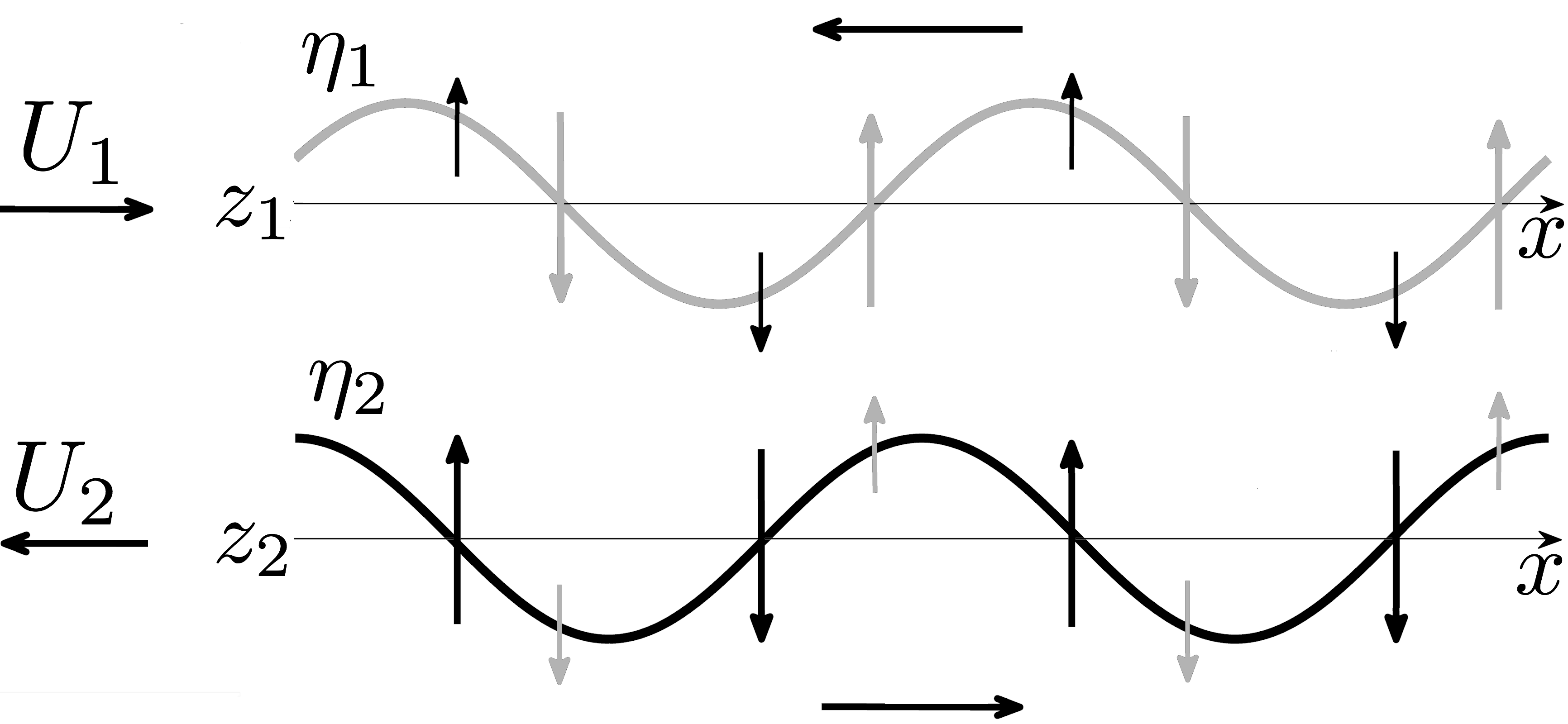
Figure 1: Schematic of the wave interaction mechanism. The interfacial deformation and associated vertical velocity of each wave are shown by the same colour. Interaction imposes an additional vertical velocity (shown by a different colour). The horizontal arrow associated with a wave indicates the intrinsic wave propagation direction. Both waves counter-propagate, i.e. move opposite to the background velocity at that location.

For reasons that will become evident in §4 we have used the subscript NM, which is short for “normal-mode”. Eq. (38) reveals that the equilibrium points exist only if

$$\left|\left\{\frac{\upomega_{1}+\upomega_{2}-\alpha\left(U_{1}-U_{2}\right)}{2\sqrt{\upomega_{1}\upomega_{2}}}\right\}e^{\alpha\left|z_{1}-z_{2}\right|}\right|\leq 1.$$ (39)

It might appear that $\Phi=n\pi$, where $n=\{-1,0,1\}$, trivially satisfies the steady state condition. Although (34) is satisfied, substitution of $\Phi=n\pi$ in (35) yields only one valid expression of $R$, which is (37). Any other expression violates (39) and yields imaginary solutions of $R$ for all $\alpha>0$.

The linear behaviour of the dynamical system around the equilibrium points is of interest. To understand this behaviour, we evaluate the Jacobian matrix, $\mathcal{J}$, at the equilibrium points:

$$\mathcal{J}\left(R_{NM},\pm\Phi_{NM}\right)=-2\sqrt{\upomega_{1}\upomega_{2}}e^{-\alpha\left|z_{1}-z_{2}\right|}\left[\begin{array}[]{cc}\sin\left(\pm\Phi_{NM}\right)&0\\ 0&\sin\left(\pm\Phi_{NM}\right)\end{array}\right].$$ (40)

Eq. (40) shows that the two eigenvalues corresponding to each equilibrium point are equal. Further analysis reveals that every vector at the equilibrium point is an eigenvector. The equilibrium point $(R_{NM},\Phi_{NM})$ produces negative eigenvalues (assuming $0\leq\Phi_{NM}\leq\pi$), while the eigenvalues corresponding to $(R_{NM},-\Phi_{NM})$ are positive. The dynamical system represented by (34)-(35) is therefore “source-sink” type. This means that a point in the phase space will move away from the “source node” $(R_{NM},-\Phi_{NM})$, and following a unique trajectory, will finally converge to the “sink node” $(R_{NM},\Phi_{NM})$.

In summary, WIT provides an understanding of hydrodynamic instability from two different perspectives - wave interaction and dynamical systems. According to the former, exponentially growing instabilities signify resonant interaction between two waves. From dynamical systems point of view, resonance implies a “steady state or equilibrium condition” ($\dot{\Phi}=0$ and $\dot{R}=0$). The wave interaction interpretation of each of the two components of the equilibrium condition is as follows:

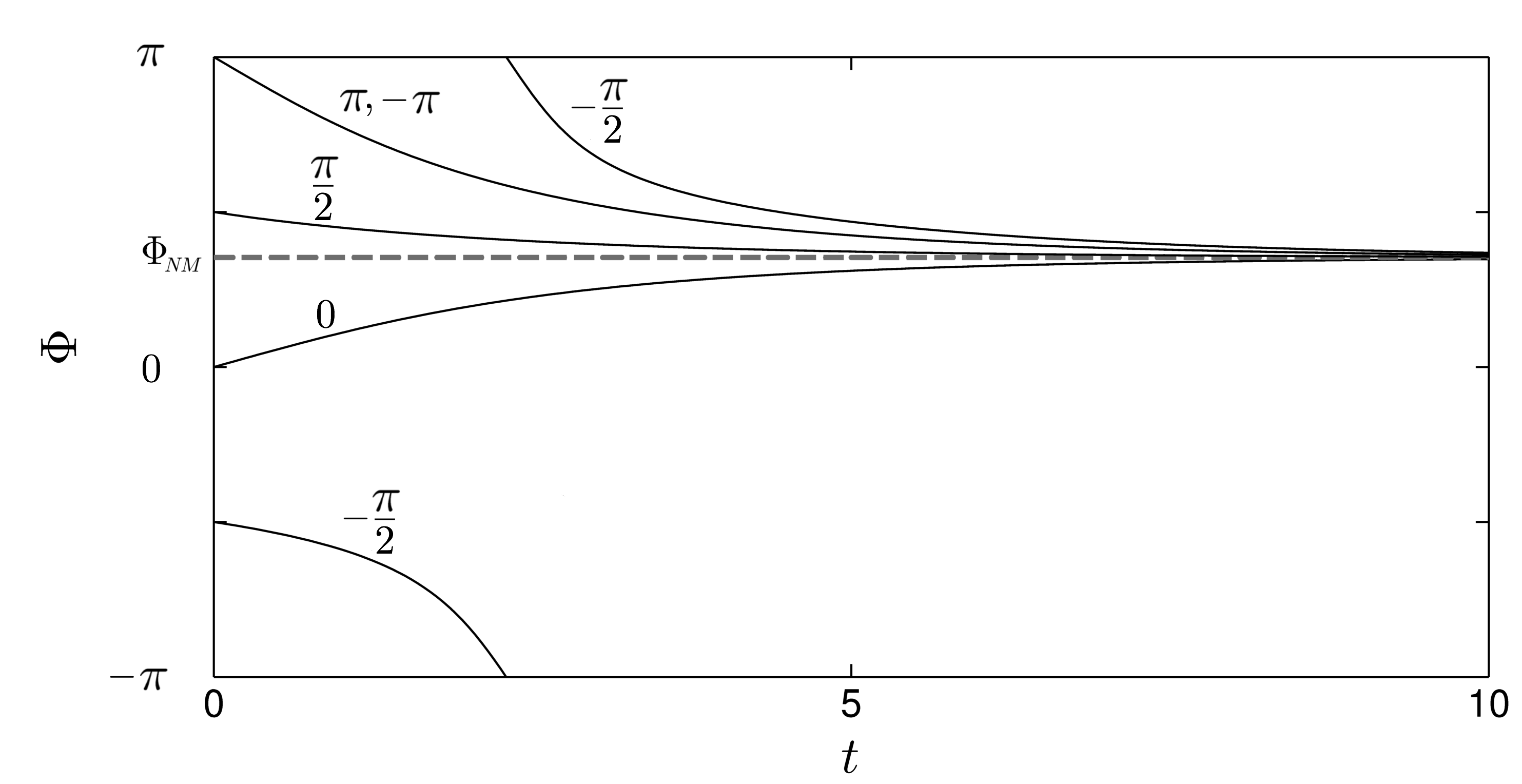
(a)

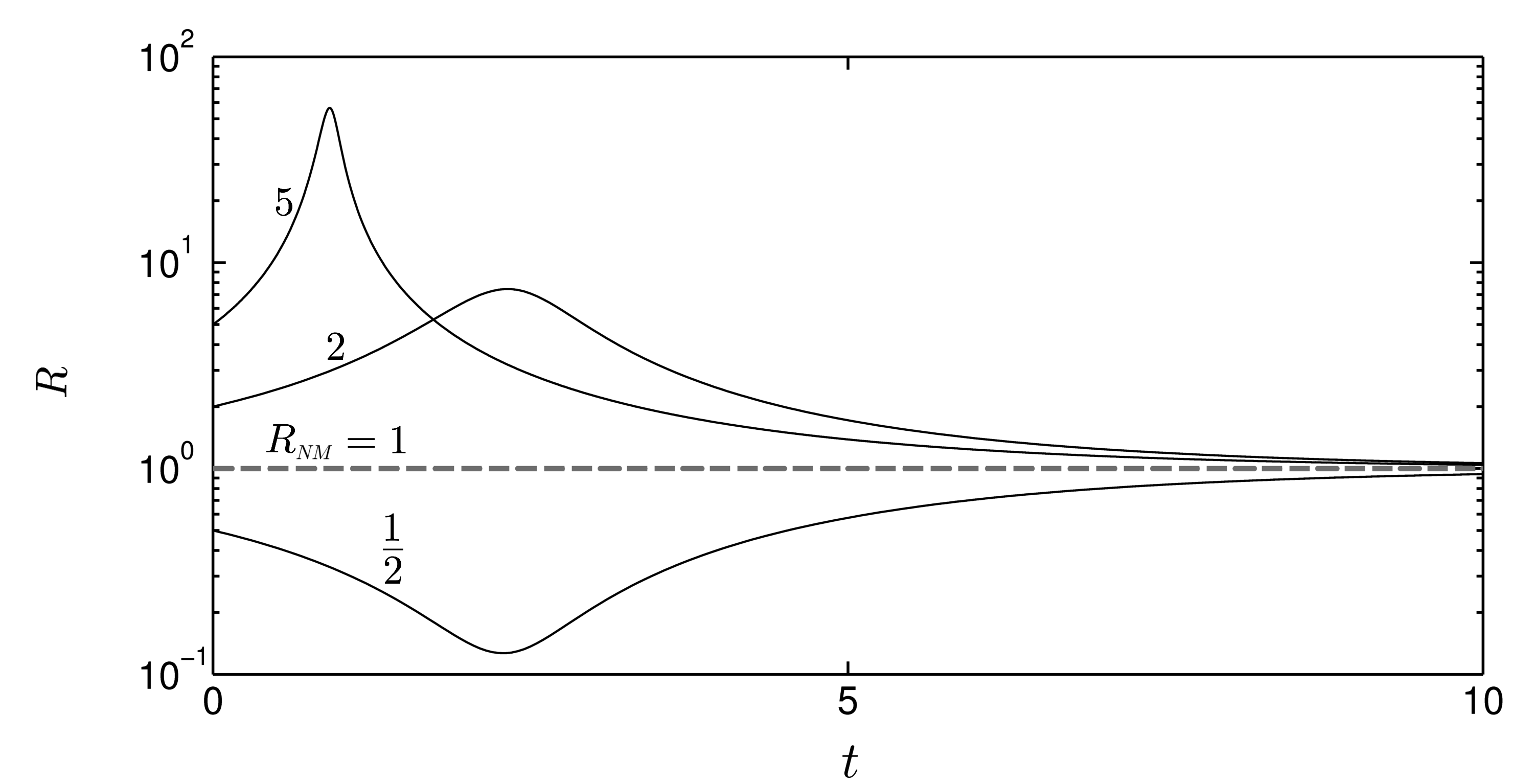
(b)

Figure 2: Any initial condition $(R_{0},\Phi_{0})$ finally yields the resonant configuration $(R_{NM},\Phi_{NM})$, provided (39) is satisfied. The case depicted here is KH instability (interaction between two vorticity waves) corresponding to $\alpha=0.4$. Any other shear instability will show qualitatively similar characteristics. (a) $\Phi$ versus $t$ corresponding to $\Phi_{0}=-\pi,-\pi/2,0,\Phi_{NM},\pi/2$ and $\pi$. The value of $R_{0}$ is held constant, and is equal to $2$. (b) $R$ versus $t$ corresponding to $R_{0}=1/2,1(R_{NM}),2$ and $5$. The value of $\Phi_{0}$ is held constant, and is equal to $-\pi/2$.

(a)

Phase-Locking or $\dot{\Phi}=0$: Reduction in the phase-speed of each wave occurs through the interaction mechanism - the vertical velocity field produced by the distant wave acts so as to diminish the phase-speed of the given wave. Furthermore, if the waves are “counter-propagating” (meaning, the direction of $c_{i}^{intr}$ is opposite to the background flow), the background flow causes an additional reduction in the phase-speed. Both wave interaction and counter-propagation work synergistically until the two waves become “phase-locked”, i.e.  stationary relative to each other ($\dot{\Phi}=0$). The phase-shift at the phase-locked state, $\Phi_{NM}$, is a unique angle dictated by the physical parameters of the system, as evident from (38). Any arbitrary initial condition (say $R=R_{0}$ and $\Phi=\Phi_{0}$) finally leads to phase-locking, as evident from figure 2(a), provided (39) is satisfied. When the condition (39) is not satisfied, the interaction is too weak to cause phase locking. The two waves continue moving in opposite directions, hence the phase-shift angle oscillates between $[0,2\pi]$ (for example see figure 3(d)).

(b)

Mutual Growth or $\dot{R}=0$: Not only the two waves lock in phase, they also lock in amplitude, producing the unique steady state amplitude-ratio $R_{NM}$; see figure 2(b). Eq. (34) reveals that $\dot{R}=0$ implies  $\gamma_{1}=\gamma_{2}$, which in turn signifies resonance between the two waves. Furthermore, (30) and (32) imply that at steady state $\gamma_{1}=\gamma_{2}=\mathrm{constant}$, meaning that the wave amplitudes grow at an exponential rate.

4 Modal and non-modal analysis

In the previous section we used WIT and dynamical systems theory to describe multi-layered inviscid hydrodynamic instabilities in terms of interacting interfacial waves. We found that the “equilibrium condition” of the dynamical system basically signifies the “resonant condition” of WIT. A question which naturally arises is “what do these conditions mean in terms of conventional hydrodynamic stability theory?” In this section we will draw parallels between WIT (and the dynamical systems formulation) and eigenanalysis and Singular Value Decomposition (SVD), which are conventionally used to study modal and non-modal instabilities, respectively.

4.1 Eigenanalysis and SVD

The linearized kinematic condition with two interfaces, (22)-(23), can be written in the matrix form by expressing $w_{i}$ in terms of $\eta_{i}$ (by invoking the definition of $\upomega_{i}$), and imposing the condition for counter-propagation ($\triangle\phi_{11}=\pi/2$ and $\triangle\phi_{22}=-\pi/2$):

$${\frac{\partial\boldsymbol{\eta}}{\partial t}=\boldsymbol{\mathcal{M}\eta}},$$ (41)

where

$$\boldsymbol{\eta}=\left[\begin{array}[]{c}\eta_{1}\\ \eta_{2}\end{array}\right]\,\,\,\,\,\,\,\,\,\textrm{and}\,\,\,\,\,\,\,\,\boldsymbol{\mathcal{M}}=-i\left[\begin{array}[]{cc}\alpha U_{1}-\upomega_{1}&\upomega_{2}e^{-\alpha\left|z_{1}-z_{2}\right|}\\ -\upomega_{1}e^{-\alpha\left|z_{1}-z_{2}\right|}&\alpha U_{2}+\upomega_{2}\end{array}\right].$$ (42)

Eq. (41) represents the first order perturbation dynamics, and $\boldsymbol{\mathcal{M}}$ is the linearized dynamical operator. Since our dynamical system is autonomous $\boldsymbol{\mathcal{M}}$ is time independent, and the solution is explicit:

$$\boldsymbol{\eta}\left(t\right)=e^{\boldsymbol{\mathcal{M}}t}\boldsymbol{\eta}\left(0\right)=\left[\boldsymbol{P}e^{\boldsymbol{L}t}\boldsymbol{P}^{-1}\right]\boldsymbol{\eta}\left(0\right)=\left[\boldsymbol{\mathcal{U}}\boldsymbol{\Sigma}\boldsymbol{V}^{\dagger}\right]\boldsymbol{\eta}\left(0\right).$$ (43)

The matrix exponential $e^{\boldsymbol{\mathcal{M}}t}$ in the above equation is the propagator matrix, which advances the system in time. The transient dynamics of the system is solely governed by the normality of $\boldsymbol{\mathcal{M}}$, i.e. whether or not $\boldsymbol{\mathcal{M}}$ commutes with its Hermitian transpose ${\boldsymbol{\mathcal{M}}^{\dagger}}$ Farrell & Ioannou (1996). If they commute ($\boldsymbol{\mathcal{M}}\boldsymbol{\mathcal{M}}^{\dagger}=\boldsymbol{\mathcal{M}}^{\dagger}\boldsymbol{\mathcal{M}}$) then $\boldsymbol{\mathcal{M}}$ is normal and has complete set of orthogonal eigenvectors. In this case the dynamics can be fully understood from the eigendecomposition of the propagator. This basically means expressing $e^{\boldsymbol{\mathcal{M}}t}$ as $\boldsymbol{P}e^{\boldsymbol{L}t}\boldsymbol{P}^{-1}$, where $\boldsymbol{L}$ is a diagonal matrix containing the complex eigenvalues $\lambda$ of $\boldsymbol{\mathcal{M}}$ (arranged by the real part of the eigenvalues in the descending order of magnitude), and $\boldsymbol{P}$ is the corresponding matrix of eigenvectors. Alternatively if $\boldsymbol{\mathcal{M}}$ is non-normal, the interaction between the discrete non-orthogonal modes of $\boldsymbol{\mathcal{M}}$ produces non-normal growth processes. Non-normality can be understood through SVD of the propagator. SVD is a generalized matrix factorization technique and matches eigendecomposition only when $\boldsymbol{\mathcal{M}}$ is Hermitian ($\boldsymbol{\mathcal{M}}=\boldsymbol{\mathcal{M}}^{\dagger}$). SVD of the propagator yields $\boldsymbol{\mathcal{U}}\boldsymbol{\Sigma}\boldsymbol{V}^{\dagger}$, where $\boldsymbol{\mathcal{U}}$ contains the eigenvectors of $e^{\boldsymbol{\mathcal{M}}t}e^{\boldsymbol{\mathcal{M}}^{\dagger}t}$, $\boldsymbol{V}$ contains the eigenvectors of $e^{\boldsymbol{\mathcal{M}}^{\dagger}t}e^{\boldsymbol{\mathcal{M}}t}$, and $\boldsymbol{\Sigma}$ is a diagonal matrix containing the singular values ($\sigma$, which are real and positive) arranged in the descending order of magnitude. If $\boldsymbol{\mathcal{M}}$ commutes with its Hermitian transpose, then $\sigma_{max}=e^{\Re(\lambda_{max})t}$. Otherwise $\sigma_{max}>e^{\Re(\lambda_{max})t}$, implying that growth-rate higher than the least stable normal-mode is possible Farrell & Ioannou (1996).

4.1.1 Eigenanalysis

If $\boldsymbol{\mathcal{M}}$ is a normal matrix, then eigendecomposition of the propagator matrix is sufficient to capture the dynamics. If $\boldsymbol{\mathcal{M}}$ is non-normal, then eigenanalysis captures the asymptotic dynamics only for large times.

The eigenvalues of the matrix $\boldsymbol{\mathcal{M}}$ are as follows:

$$\lambda_{\pm}=-\frac{{\rm i}}{2}\left[\alpha\left(U_{1}+U_{2}\right)-\left(\upomega_{1}-\upomega_{2}\right)\right]\pm\frac{1}{2}\sqrt{\mathscr{D}},$$ (44)

where $\mathscr{D}=4\upomega_{1}\upomega_{2}e^{-2\alpha\left|z_{1}-z_{2}\right|}-\left[\alpha\left(U_{1}-U_{2}\right)-\left(\upomega_{1}+\upomega_{2}\right)\right]^{2}$. Normal-mode instability can only occur if $\mathscr{D}>0$. This basically gives rise to the condition (39), implying that (39) denotes the necessary and sufficient (N&S) condition for exponentially growing instabilities in idealized (broken-line profiles), homogeneous and stratified, inviscid shear layers. The unstable eigenvalues of (44) can therefore be written as

$$\lambda_{\pm}=-\frac{{\rm i}}{2}\left[\alpha\left(U_{1}+U_{2}\right)-\left(\upomega_{1}-\upomega_{2}\right)\right]\pm\sqrt{\upomega_{1}\upomega_{2}}e^{-\alpha\left|z_{1}-z_{2}\right|}\sin\left(\Phi_{NM}\right).$$ (45)

The positive and negative eigenvalues respectively imply growing and decaying normal-modes of the discrete spectrum. There is a direct relation between the normal-modes and the resonant condition of WIT (or the equilibrium condition of the dynamical system (34)-(35)). Each equilibrium point corresponds to a normal-mode : $(R_{NM},\Phi_{NM})$ corresponds to the growing normal-mode (signifying exponential growth $e^{\Re(\lambda_{+})t}$), and $(R_{NM},-\Phi_{NM})$ corresponds to the decaying normal-mode (signifying exponential decay $e^{\Re(\lambda_{-})t}$). An analogy can be drawn with a system of two coupled harmonic oscillators. Such a system has two normal-modes of vibration, the in-phase synchronization mode (zero phase-shift) and the anti-phase synchronization mode (phase-shift of $\pi$). The in-phase and anti-phase modes are respectively analogous to the growing and decaying normal-modes of WIT.

WIT is only relevant to problems where the discrete spectrum is of primary interest, and the effect of the continuous spectrum can be neglected. In other words, the applicability of WIT is restricted to idealized multi-layered profiles. Real profiles are continuous and their eigenanalysis yields a continuous spectrum. Although the continuous spectrum consists of neutral modes, they interact to produce sheared disturbances. Such disturbances can be obtained by artificially changing the vorticities of fluid elements by small amounts, imposing a sinusoidal streamwise dependence, and then letting the system evolve freely. This spectrum crucially contributes to the non-modal instability processes, and is responsible for large transient growths.

4.1.2 SVD analysis

If $\boldsymbol{\mathcal{M}}$ is non-normal, then eigenanalysis fails to capture the dynamics in the limit $t\rightarrow 0$. To understand the short-term dynamics, one needs to perform SVD analysis. The eigenvalue matrix of $e^{\boldsymbol{\mathcal{M}}t}e^{\boldsymbol{\mathcal{M}}^{\dagger}t}$ (or $e^{\boldsymbol{\mathcal{M}}^{\dagger}t}e^{\boldsymbol{\mathcal{M}}t}$) is equal to $\boldsymbol{\Sigma}^{2}$; the maximum eigenvalue of $\boldsymbol{\Sigma}$ is key in determining the transient dynamics. In the limit $t\rightarrow 0$, Taylor expansion of $e^{\boldsymbol{\mathcal{M}}^{\dagger}t}e^{\boldsymbol{\mathcal{M}}t}$ produces Farrell & Ioannou (1996):

$$e^{\boldsymbol{\mathcal{M}}^{\dagger}t}e^{\boldsymbol{\mathcal{M}}t}\approx(\boldsymbol{I}+\boldsymbol{\mathcal{M}}^{\dagger}t+\ldots)(\boldsymbol{I}+\boldsymbol{\mathcal{M}}t+\ldots)$$

$$=\boldsymbol{I}+(\boldsymbol{\mathcal{M}}+\boldsymbol{\mathcal{M}}^{\dagger})t+O(t^{2}),\,\,\,\,\,\,\,\,\,\,\,\,\,\,\,\,$$ (46)

where $\boldsymbol{I}$ is the identity matrix. The maximum eigenvalue of $\frac{1}{2}(\boldsymbol{\mathcal{M}}+\boldsymbol{\mathcal{M}}^{\dagger})$ (which is known as the numerical abscissa of $\boldsymbol{\mathcal{M}}$) and its associated eigenvector provide the maximum instantaneous growth-rate and structure. The numerical abscissa is found to be

$$\sigma_{max}=\frac{1}{2}\left(\upomega_{1}+\upomega_{2}\right)e^{-\alpha\left|z_{1}-z_{2}\right|}.$$ (47)

It is straight-forward to check that

$$\frac{\sigma_{max}}{\Re\left(\lambda_{+}\right)}\geq\frac{1}{\sin\left(\Phi_{NM}\right)}\Rightarrow\sigma_{max}\geq\Re\left(\lambda_{+}\right).$$ (48)

4.2 Non-modal growth

The non-normality of the system can give rise to transient energy amplification. Even when the waves are decaying, the non-orthogonal superposition of eigenvectors may lead to short-time growth of energy (or some other norm). For the non-modal analysis we have chosen $E=\upomega_{1}A_{\eta_{1}}^{2}+\upomega_{2}A_{\eta_{2}}^{2}$ as a suitable norm. The time evolution of $E$ is used to indicate the growth (or decay) of the system, and is calculated as follows:

$$\dot{E}=2\upomega_{1}A_{\eta_{1}}\dot{A}_{\eta_{1}}+2\upomega_{2}A_{\eta_{2}}\dot{A}_{\eta_{2}}=4A_{\eta_{1}}A_{\eta_{2}}\upomega_{1}\upomega_{2}e^{-\alpha\left|z_{1}-z_{2}\right|}\sin\left(\Phi\right).$$ (49)

The rightmost side of (49) is obtained by substituting (30) and (32). Furthermore, the inequality $\left(\sqrt{\upomega_{1}}A_{\eta_{1}}-\sqrt{\upomega_{2}}A_{\eta_{2}}\right)^{2}\geq 0\Rightarrow\upomega_{1}A_{\eta_{1}}^{2}+\upomega_{2}A_{\eta_{2}}^{2}\geq 2\sqrt{\upomega_{1}\upomega_{2}}A_{\eta_{1}}A_{\eta_{2}}$. Hence

$$\dot{E}\leq 2E\sqrt{\upomega_{1}\upomega_{2}}e^{-\alpha\left|z_{1}-z_{2}\right|}\sin\left(\Phi\right).$$ (50)

$\dot{E}$ is maximum when $\left(\sqrt{\upomega_{1}}A_{\eta_{1}}-\sqrt{\upomega_{2}}A_{\eta_{2}}\right)^{2}=0\Rightarrow R=\sqrt{\upomega_{2}/\upomega_{1}}$. The corresponding $E$ is $E_{m}=2\upomega_{1}A_{\eta_{1}}^{2}=2\upomega_{2}A_{\eta_{2}}^{2}$. The time evolution of $\dot{E}_{m}$ is given by

$$\dot{E}_{m}=2E_{m}\sqrt{\upomega_{1}\upomega_{2}}e^{-\alpha\left|z_{1}-z_{2}\right|}\sin\left(\Phi\right).$$ (51)

The sign of the R.H.S. of (51) dictates whether the system is growing (positive sign) or decaying (negative sign). Since only $\sin\left(\Phi\right)$ is a signed quantity, it means that the instantaneous phase-shift governs the instantaneous growth or decay. The largest instantaneous growth occurs when $\Phi=\pi/2$ (this fact can also be verified from (30) and (32)). Figure 3(a) shows an example of how $A_{\eta}$ (=$\sqrt{E_{m}/(2\upomega)}$) varies with time. During the initial period, the wave amplitude decays (since the initial phase-shift $\Phi_{0}<0$) and then grows at a rate faster than that predicted by the normal-mode theory. Eventually, the growth-rate asymptotes to that predicted by normal-mode theory. Note that the flow becomes non-linear relatively quickly, and the linear theories (e.g. WIT and normal-mode) start to deviate from the non-linear theory; see figure 3 of Guha, Rahmani & Lawrence (2013).

The amplification or gain ($G$) of the system is given by:

$$G\left(t\right)=\frac{E_{max}\left(t\right)}{E_{max}\left(0\right)}=\exp\left[2\sqrt{\upomega_{1}\upomega_{2}}e^{-\alpha\left|z_{1}-z_{2}\right|}\intop_{0}^{t}\sin\left(\Phi\right)dt^{\prime}\right].$$ (52)

The quantity $dt$ can be expressed in terms of $d\Phi$ by invoking (35). Substituting $R=\sqrt{\upomega_{2}/\upomega_{1}}$ and integrating, we obtain

$$G\left(t\right)=\left|\frac{\cos\left(\Phi_{0}\right)-Q}{\cos\left(\Phi_{t}\right)-Q}\right|,$$ (53)

where $Q=\{\upomega_{1}+\upomega_{2}-\alpha(U_{1}-U_{2})\}e^{\alpha\left|z_{1}-z_{2}\right|}/(2\sqrt{\upomega_{1}\upomega_{2}})$, and $\Phi_{t}$ is the value of $\Phi$ at $t=t$. Notice that $|Q|\leq 1$ denotes the N&S condition (39).

4.2.1 Non-modal growth when N&S condition is satisfied:

When the N&S condition is satisfied $Q=\cos(\Phi_{NM})$; see (38). Hence (53) yields

$$G\left(t\right)=\left|\frac{\sin\left(\frac{\Phi_{NM}+\Phi_{0}}{2}\right)\sin\left(\frac{\Phi_{NM}-\Phi_{0}}{2}\right)}{\sin\left(\frac{\Phi_{NM}+\Phi_{t}}{2}\right)\sin\left(\frac{\Phi_{NM}-\Phi_{t}}{2}\right)}\right|.$$ (54)

We find that $G\rightarrow\infty$ when the final phase-shift $\Phi_{t}\rightarrow\pm\Phi_{NM}$. The positive and negative values of $\Phi_{NM}$ respectively denote the sink node and the source node in phase space. Since trajectories move away from the source node, $\Phi_{t}\nrightarrow-\Phi_{NM}$ during the non-modal evolution process (for example, see figure 4(b)). The significance of the non-modal gain $G$ can be properly understood when compared with a hypothetical case in which the system undergoes modal growth between $\Phi=\Phi_{0}$ and $\Phi_{NM}$. For this we first compute the gain obtained from a normal-mode type perturbation growing over an interval $t$:

$$G_{NM}\left(t\right)=e^{2\Re\left(\lambda_{+}\right)t}=\exp\left[2\left\{\tanh^{-1}\left(\frac{\tan\left(\frac{\Phi_{t}}{2}\right)}{\tan\left(\frac{\Phi_{NM}}{2}\right)}\right)-\tanh^{-1}\left(\frac{\tan\left(\frac{\Phi_{0}}{2}\right)}{\tan\left(\frac{\Phi_{NM}}{2}\right)}\right)\right\}\right]$$

$$=\left|\frac{\sin\left(\frac{\Phi_{NM}+\Phi_{t}}{2}\right)}{\sin\left(\frac{\Phi_{NM}-\Phi_{t}}{2}\right)}\right|\left|\frac{\sin\left(\frac{\Phi_{NM}-\Phi_{0}}{2}\right)}{\sin\left(\frac{\Phi_{NM}+\Phi_{0}}{2}\right)}\right|.\,\,\,\,\,\,\,\,\,\,\,\,\,\,\,\,\,\,\,\,\,\,\,\,\,\,\,\,\,\,\,\,\,\,\,\,\,\,\,\,\,\,\,\,\,\,\,\,\,\,\,\,\,\,\,\,\,\,\,\,\,\,\,\,\,\,\,\,\,\,$$ (55)

Like $G$, the normal-mode gain $G_{NM}\rightarrow\infty$ when $\Phi_{t}\rightarrow\Phi_{NM}$. The gain-ratio $\chi\left(t\right)=G(t)/G_{NM}(t)$ is found to be

$$\chi\left(t\right)=\frac{\sin^{2}\left(\frac{\Phi_{NM}+\Phi_{0}}{2}\right)}{\sin^{2}\left(\frac{\Phi_{NM}+\Phi_{t}}{2}\right)}.$$ (56)

When $\chi>1$, the non-normal growth exceeds exponential growth within the time window $[0,t]$. For our calculations we have chosen the entire time window of non-modal evolution. Thus (56) becomes

$$\chi\left(t_{NM}\right)=\frac{\sin^{2}\left(\frac{\Phi_{NM}+\Phi_{0}}{2}\right)}{\sin^{2}\left(\Phi_{NM}\right)}.$$ (57)

Notice that unlike $G$ and $G_{NM}$, the value of $\chi$ is finite as $t\rightarrow t_{NM}$. Figure 3(b) depicts the variation of $\log(\chi)$ with $\alpha$ and $\Phi_{0}$ for KH instability. The flow is linearly unstable for $0\leq\alpha\leq 0.64$ (see §5.1). Non-modal gain exceeds modal gain by several orders of magnitude in the neighbourhood of stability boundaries. This behaviour is especially prominent near the lower boundary. The fact that substantial transient growth occurs near stability boundaries has also been observed for non-modal Holmboe instability Constantinou & Ioannou (2011). The magnitude of $\chi$ is strongly dependent on the initial condition. We observe higher values of $\chi$ when the component waves are long (smaller values of $\alpha$), and initially out of phase ($\Phi_{0}$ away from $0$). This situation reverses near the upper boundary; waves starting in-phase exhibit higher magnitudes of $\chi$.

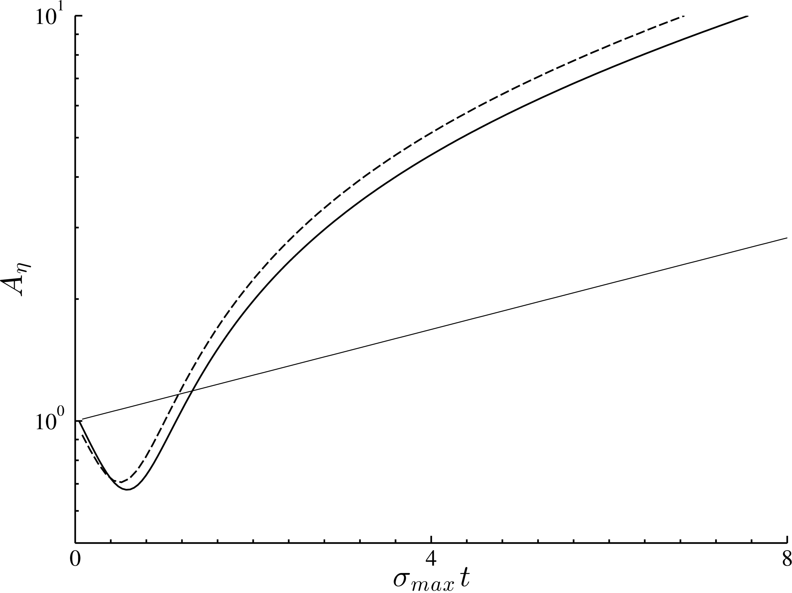
(a)

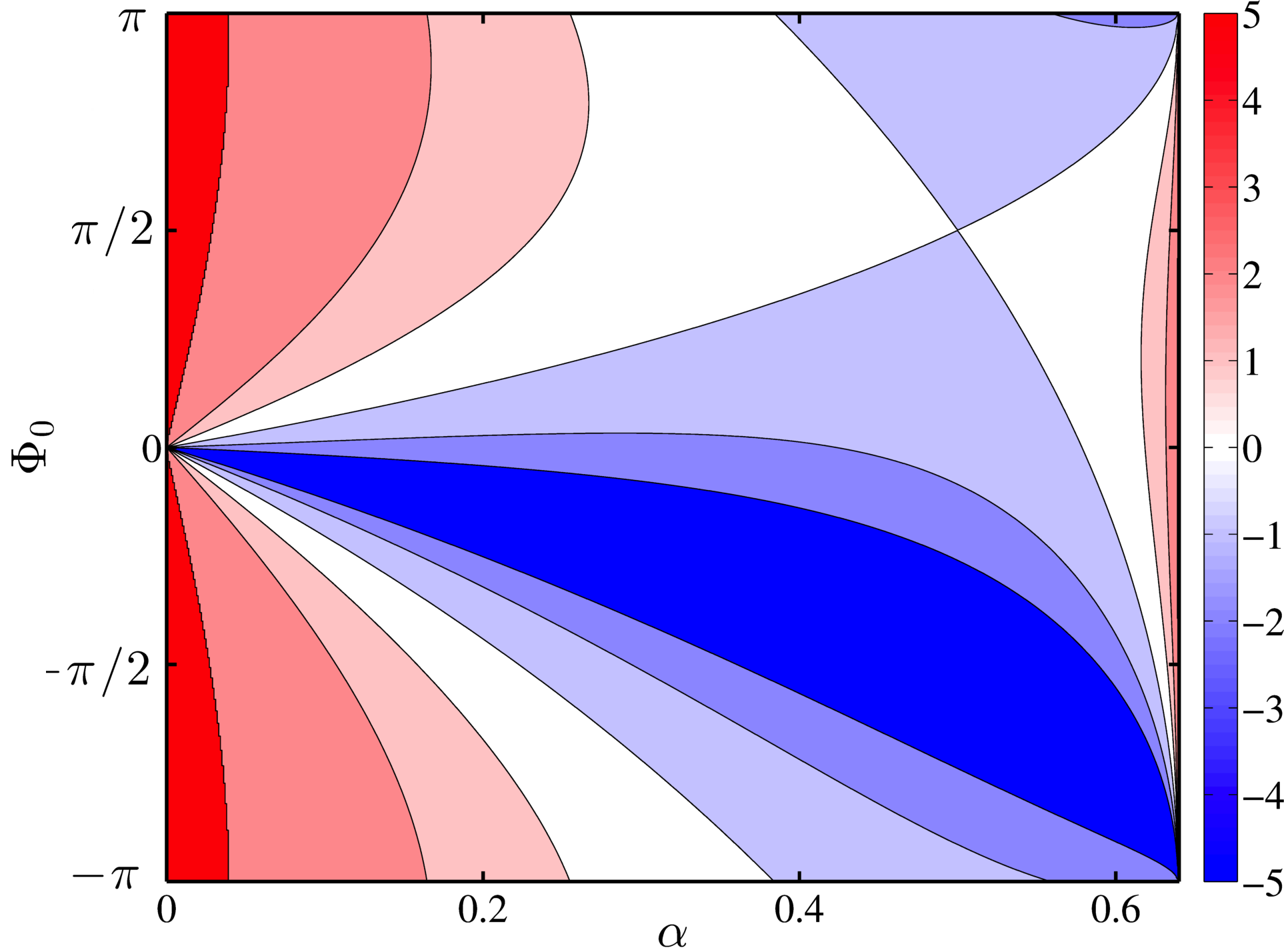
(b)

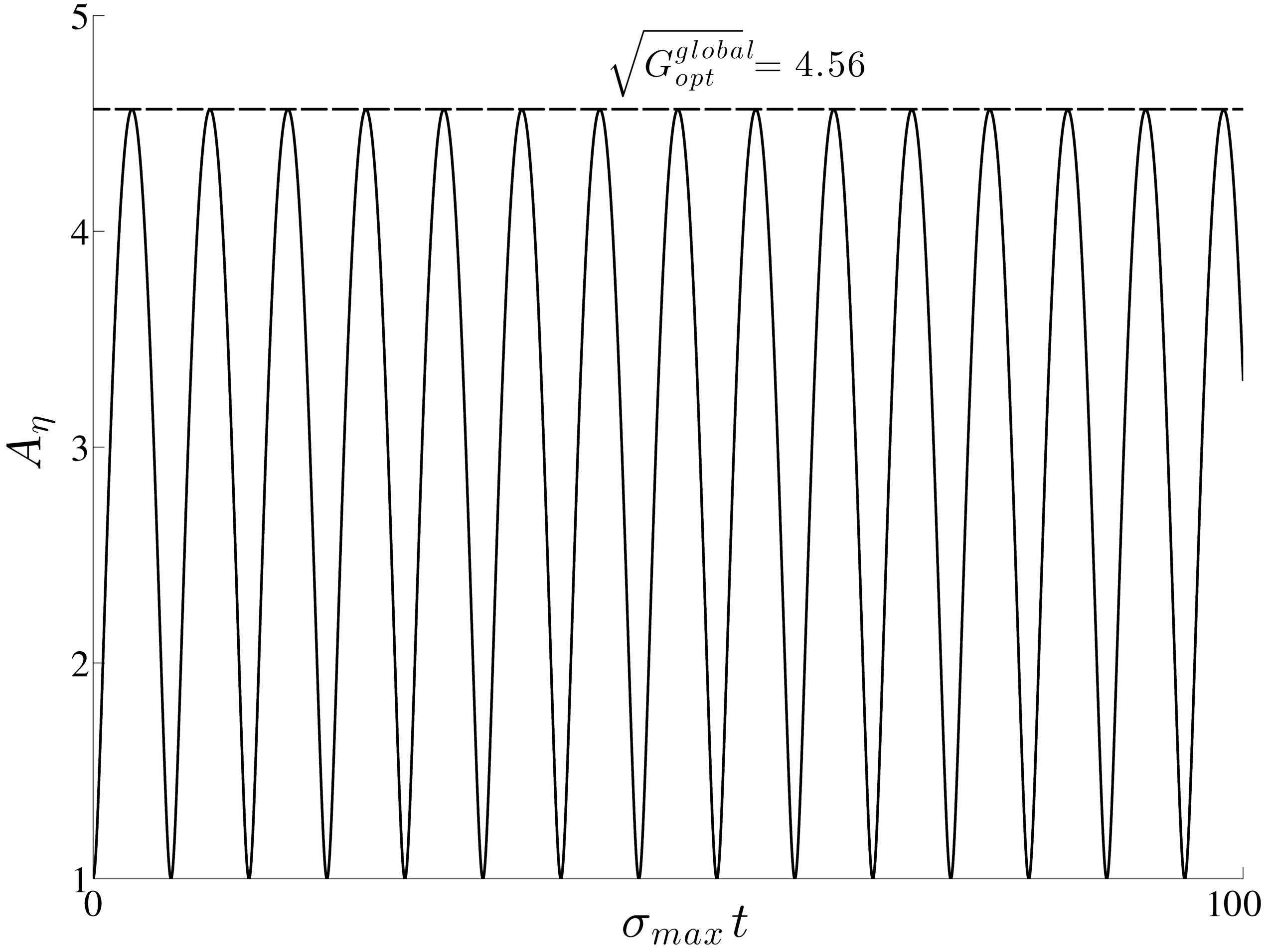
(c)

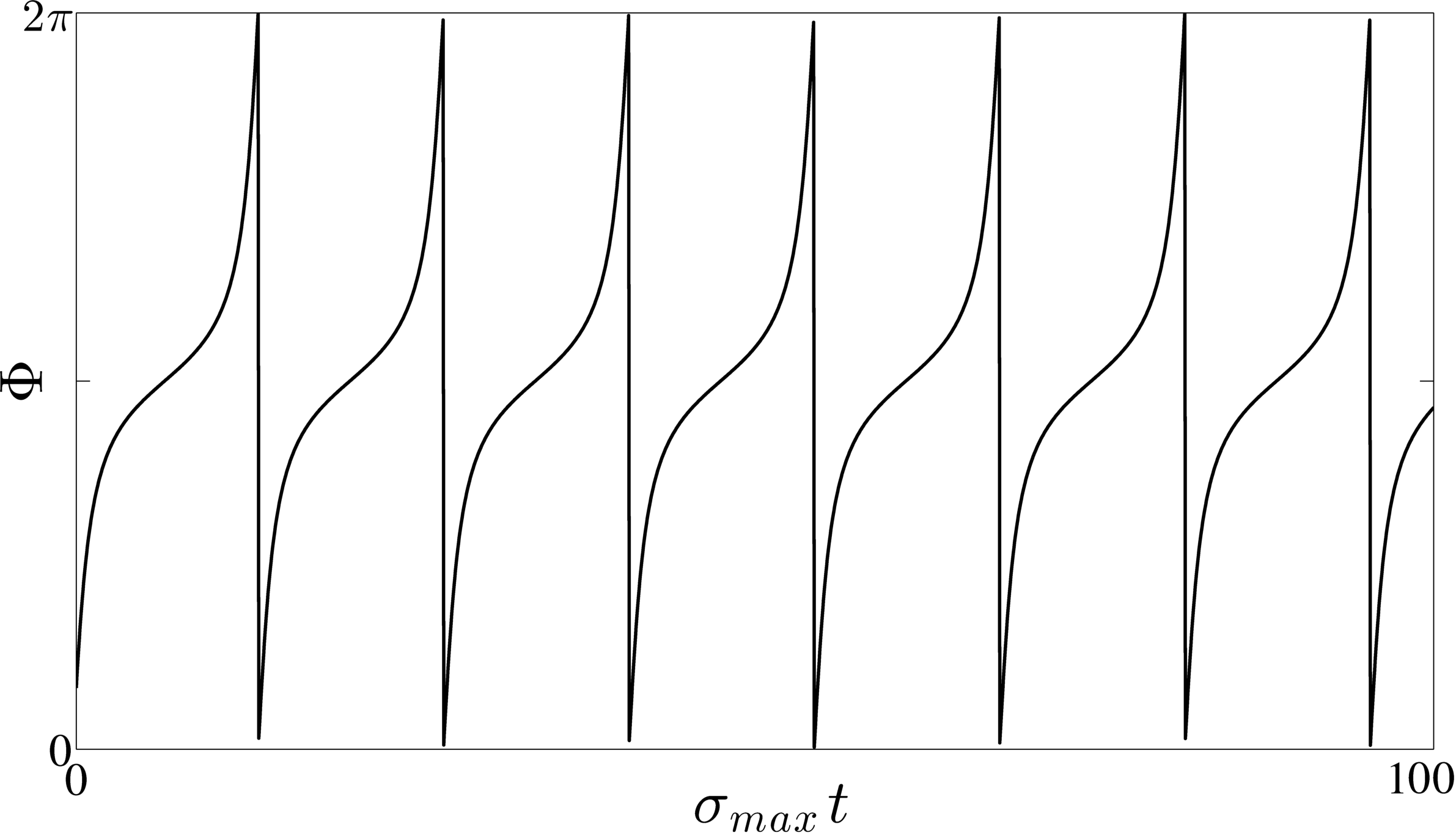
(d)

Figure 3: Different aspects of transient dynamics of KH instability: (a) Variation of wave amplitude with target time (both normalized) for $\alpha=0.0625$ and $\Phi_{0}=-\pi/2$. The bold solid curve represents WIT, and the bold dashed curve is its non-linear extension; see Guha, Rahmani & Lawrence (2013). The thin solid line represents amplitude variation predicted by the normal-mode theory. The slope of the WIT curve becomes parallel to that of the normal-mode for large times. (b) (Colour online) Plot of $\log(\chi)$ as a function of $\alpha$ and $\Phi_{0}$. Positive contour values indicate non-modal growth exceeding corresponding modal growth. (c) Variation of normalized wave amplitude with normalized target time for $\alpha=0.65$. (d) Variation of phase-shift with normalized target time for $\alpha=0.65$.

4.2.2 Non-modal growth when N&S condition is not satisfied:

When the N&S condition is not satisfied $|Q|>1$, and the flow is linearly stable according to the normal-mode theory. The amplitude of a small perturbation is therefore expected to stay constant in this region. However non-modal processes can produce transient growth in the parameter space for which the flow is deemed stable by the normal-mode analysis. This can be shown by studying the evolution of the optimal perturbation. Using SVD analysis Heifetz & Methven (2005) have shown that optimal perturbation evolves such that the final phase-shift $\Phi_{t}=\pi-\Phi_{0}$. The phase-shift is symmetric in time about $\pi/2$, maximizing $\sin\left(\Phi\right)$ in (52). Thus the optimal gain $G_{opt}$ is found to be

$$G_{opt}=\left|\frac{Q+\cos\left(\Phi_{0}\right)}{Q-\cos\left(\Phi_{0}\right)}\right|.$$ (58)

The optimal gain is maximum when $\Phi_{0}=0$, and is given by

$$G_{opt}^{global}=\frac{\left|Q\right|+1}{\left|Q\right|-1}.$$ (59)

$G_{opt}^{global}$ is known as the global optimal gain. We take KH instability as an example for studying the non-modal behaviour. The condition $|Q|>1$ in this case translates to $\alpha>0.64$ (see §5.1). From figure 3(c) we find that the perturbation amplitude corresponding to $\alpha=0.65$ grows to a maximum of $\sqrt{G_{opt}^{global}}=4.56$ times its initial value. Similar results have been obtained by Heifetz & Methven (2005), who studied the non-normal behaviour using the enstrophy norm. Figure 3(d) shows the corresponding temporal variation of its phase-shift. Unlike figure 2(a), there is no phase-locking since N&S condition is not satisfied here. Instead, the two “marginally stable” (as referred to in the classical theory) wave-modes continue to propagate in opposite directions. Hence the phase-shift oscillates between $0$ and $2\pi$.

5 Analysis of classical shear instabilities using WIT

The WIT formulation proposed in §3 is quite general in the sense that we have not prescribed the types of the constituent waves. Different kinds of shear instabilities may arise depending on the wave types. For example, the interaction between two vorticity waves results in KH instability; Taylor-Caulfield instability results from the interaction between two gravity waves in constant shear, while the interaction between a vorticity and a gravity wave produces Holmboe instability. In this section we will use WIT to analyze the three above mentioned classical examples of shear instabilities.

5.1 The Rayleigh/Kelvin-Helmholtz Instability

Let us consider a piecewise linear velocity profile

$$U\left(z\right)=\begin{cases}U_{1}&\,\,\,\,\,\,\,\,\,\,\,\,\,\,z\geq z_{1}\\ Sz&z_{2}\leq z\leq z_{1}\\ U_{2}&\,\,\,\,\,\,\,\,\,\,\,\,\,z\leq z_{2}.\end{cases}$$ (60)

This profile is a prototype of barotropic shear layers occurring in many geophysical and astrophysical flows Guha, Rahmani & Lawrence (2013). It supports two vorticity waves, one at $z_{1}$ and the other at $z_{2}$. The shear $S=(U_{1}-U_{2})/(z_{1}-z_{2})$. We nondimensionalize the problem by choosing a length scale $h=(z_{1}-z_{2})/2$ and a velocity scale $\Delta U=(U_{1}-U_{2})/2$. In a reference frame moving with the mean flow $\bar{U}=(U_{1}+U_{2})/2$, the non-dimensional velocity profile becomes

$$U\left(z\right)=\begin{cases}\,\,\,\,1&\,\,\,\,\,\,\,\,\,\,\,\,\,\,\,\,z\geq 1\\ \,\,\,\,z&-1\leq z\leq 1\\ -1&\,\,\,\,\,\,\,\,\,\,\,\,\,\,\,z\leq-1.\end{cases}$$ (61)

This profile, along with the vorticity waves, is shown in figure 4(a). The top wave is left moving while the bottom wave moves to the right.

Using the classical normal-mode theory Rayleigh (1880) showed that the profile in (61) is linearly unstable for $0\leq\alpha\leq 0.64$. This instability is often referred to as the “Rayleigh’s shear instability”. However we have addressed it as the “Rayleigh/Kelvin-Helmholtz” instability, and used the acronym “KH”.

Figure 4(a) reveals that the KH instability can be analyzed using WIT framework. Since the two waves involved in the KH instability are vorticity waves, we substitute (14) in (30)-(33), and after non-dimensionalization we obtain

$$\gamma_{1}=\frac{1}{2R}e^{-2\alpha}\sin\Phi$$ (62)

$$c_{1}=1-\frac{1}{2\alpha}\left[1-\frac{1}{R}e^{-2\alpha}\cos\Phi\right]$$ (63)

$$\gamma_{2}=\frac{R}{2}e^{-2\alpha}\sin\Phi$$ (64)

$$c_{2}=-1+\frac{1}{2\alpha}\left[1-Re^{-2\alpha}\cos\Phi\right].$$ (65)

Eqs. (62)-(65) provide a non-modal description of KH instability. The equation-set is isomorphic to (14a)-(14d) of Heifetz, Bishop & Alpert (1999) and homomorphic to (7a)-(7d) of Davies & Bishop (1994). While the equation-set described by Heifetz, Bishop & Alpert (1999) shows how counter-propagating Rossby wave interactions lead to barotropic shear instability, the equation-set formulated by Davies & Bishop (1994) shows how baroclinic instability is produced through the interaction of temperature edge waves.

The generalized non-linear dynamical system given by (34)-(35) in this case translates to

$$\dot{R}=\frac{1}{2}\left(1-R^{2}\right)e^{-2\alpha}\sin\Phi$$ (66)

$$\dot{\Phi}=\left(2\alpha-1\right)+\frac{1}{2}\left(R+\frac{1}{R}\right)e^{-2\alpha}\cos\Phi.$$ (67)

The equilibrium points of this system are $(R_{NM},\pm\Phi_{NM})$, where

$$R_{NM}=1$$ (68)

$$\Phi_{NM}=\cos^{-1}\left[\left(1-2\alpha\right)e^{2\alpha}\right].$$ (69)

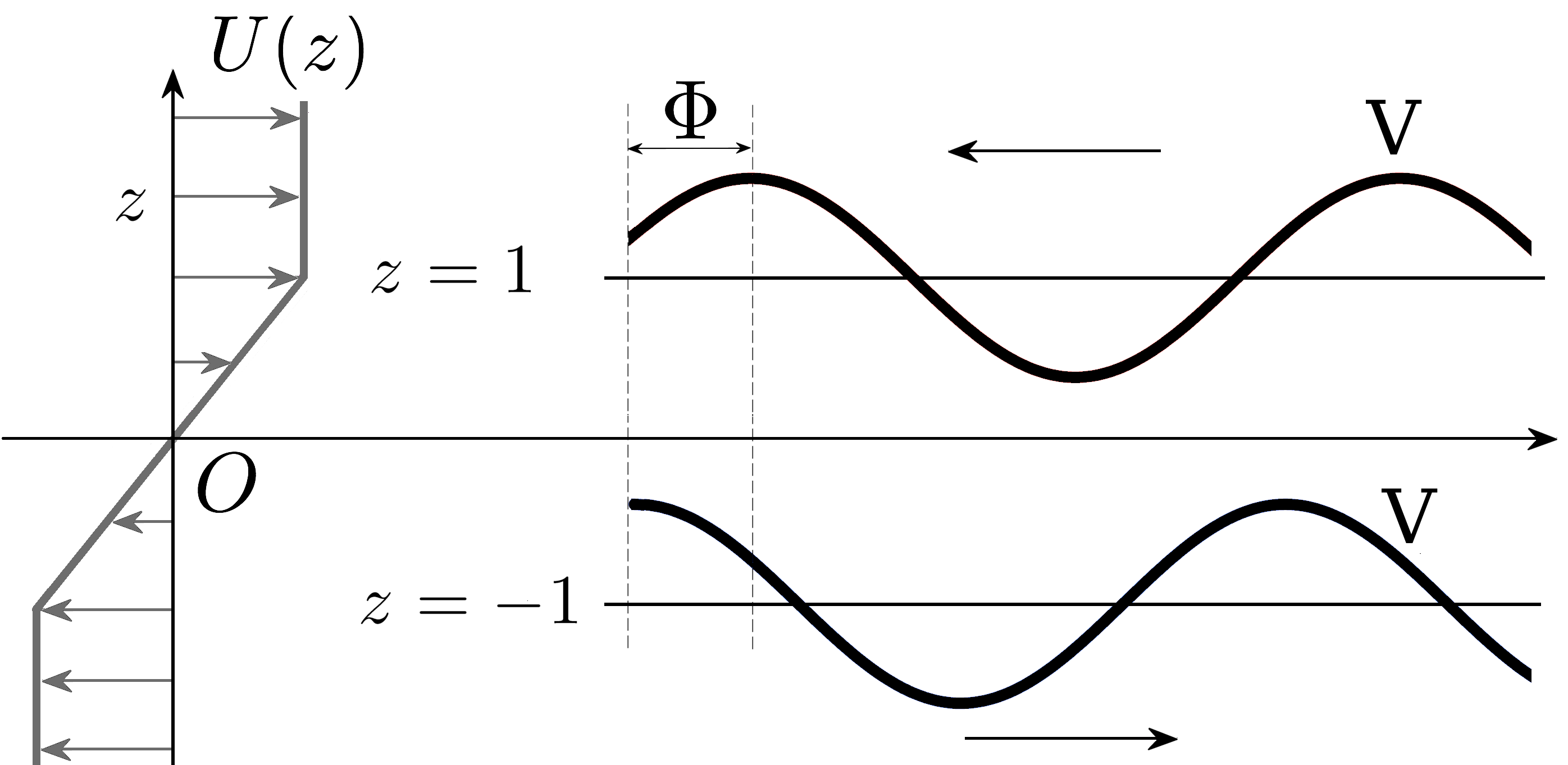
(a)

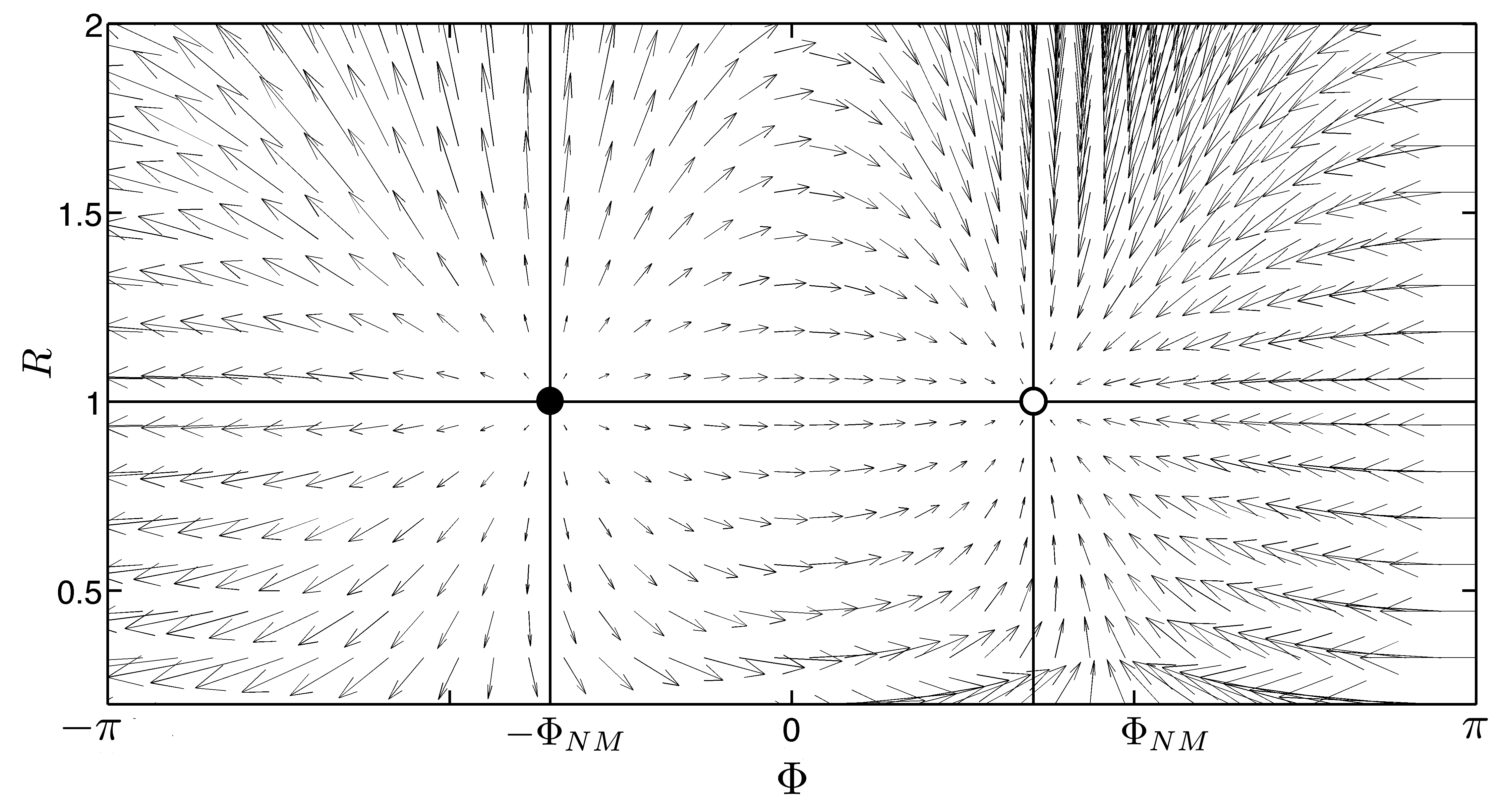
(b)

Figure 4: (a) The setting leading to the KH instability. The velocity profile in (61) is shown on the left, while the vorticity waves (marked by “V”) are shown on the right. (b) Phase portrait of KH instability corresponding to $\alpha=0.4$. The system has two equilibrium points - the source node (•) and the sink node $(\circ)$.

The phase portrait is shown in figure 4(b). It confirms that the dynamical system is indeed of source-sink type, as predicted in §3.

The N&S condition for instability expressed via (39) in this case reads

$$-1\leq\left(1-2\alpha\right)e^{2\alpha}\leq 1\,\,\,\,\mathsf{\mathrm{implying}}\,\,\,\,0\leq\alpha\leq 0.64.$$ (70)

The range of unstable wavenumbers obtained from the above equation corroborates Rayleigh’s normal-mode analysis. Normal-mode theory also shows that the wavenumber of maximum growth is $\alpha_{max}=0.4$. The same answer can be obtained from WIT by imposing the normal-mode condition and maximizing $\gamma_{1}$ or $\gamma_{2}$ with respect to $\alpha$.

The fact that KH instability develops into a standing wave instability can be verified by applying the normal-mode condition in (63) and (65). Performing the necessary steps we find $c_{1}=c_{2}=0$, i.e. the waves became stationary after phase-locking. The waves stay in this configuration and grow exponentially, hence the shear layer grows in size. The growth process eventually becomes non-linear, and the shear layer modifies into elliptical patches of constant vorticity Guha, Rahmani & Lawrence (2013).

5.2 The Taylor-Caulfield Instability

Let us consider a uniform shear layer with two density interfaces

$$U(z)=Sz\,\,\,\,\,\,\,\,\mathrm{and}\,\,\,\,\,\,\,\,\rho\left(z\right)=\begin{cases}\rho_{0}-\frac{\Delta\rho}{2}&\,\,\,\,\,\,\,\,\,\,\,\,\,\,z\geq z_{1}\\ \rho_{0}&z_{2}\leq z\leq z_{1}\\ \rho_{0}+\frac{\Delta\rho}{2}&\,\,\,\,\,\,\,\,\,\,\,\,\,z\leq z_{2}.\end{cases}$$ (71)

The shear $S$ is constant. We choose $\Delta\rho/2$ as the density scale, $h=(z_{1}-z_{2})/2$ as the length scale, and thereby nondimensionalize (71). The physical state of the system is determined by the competition between density stratification and shear, the non-dimensional measure of which is given by the Bulk Richardson number $J=g^{\prime}/(hS^{2})$, where $g^{\prime}=g(\Delta\rho/2)/\rho_{0}$ is the reduced gravity, and $\rho_{0}$ is the reference density. The dimensionless velocity and density profiles therefore become

$$U(z)=z\,\,\,\,\,\,\,\,\mathrm{and}\,\,\,\,\,\,\,\,\,\rho\left(z\right)=\begin{cases}-1&\,\,\,\,\,\,\,\,\,\,\,\,\,\,\,\,z\geq 1\\ \,\,\,\,0&-1\leq z\leq 1\\ \,\,\,\,1&\,\,\,\,\,\,\,\,\,\,\,\,\,\,\,\,z\leq-1.\end{cases}$$ (72)

This flow configuration is shown in figure 5(a). Notice that a homogeneous flow with $U(z)=z$ is linearly stable. Moreover, a stationary fluid having a density distribution as in (72) is gravitationally stable. Surprisingly, the flow obtained by superimposing the two stable configurations is linearly unstable. Taylor (1931) was the first to report and provide a detailed theoretical analysis of this rather non-intuitive instability. The first experimental evidence of this instability was provided by Caulfield et al. (1995). Following Carpenter et al. (2013) we refer to it as the “Taylor-Caulfield (TC) instability”. The interplay between the background shear and the gravity waves existing at the density interfaces produce the destabilizing effect. Taylor (1931) found that for each value of $J$, there exists a band of unstable wavenumbers (and vice-versa), shown in figure 5(b). This unstable range is given by (see Howard & Maslowe (1973) or (2.154) of Sutherland (2010)):

$$\frac{2\alpha}{1+e^{-2\alpha}}\leq J\leq\frac{2\alpha}{1-e^{-2\alpha}}.$$ (73)

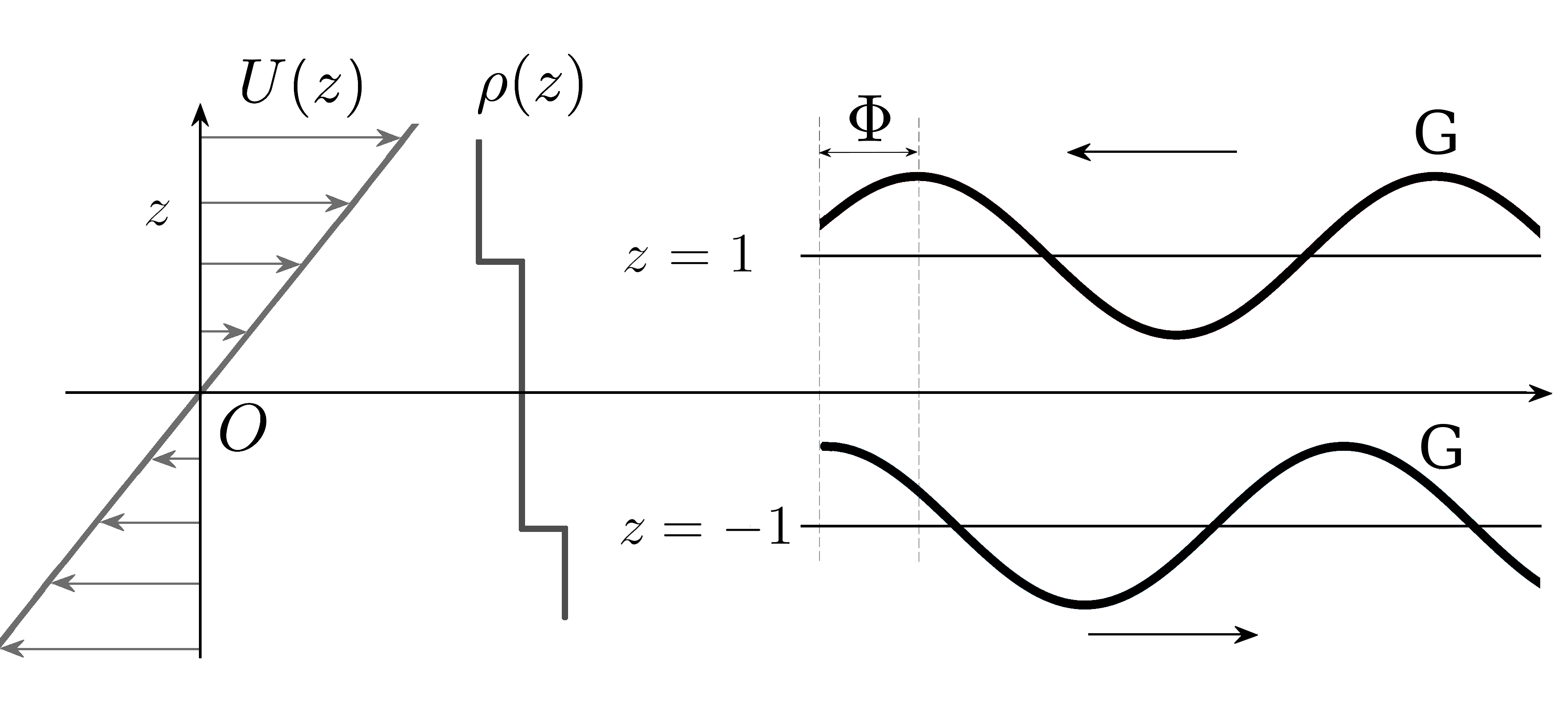
(a)

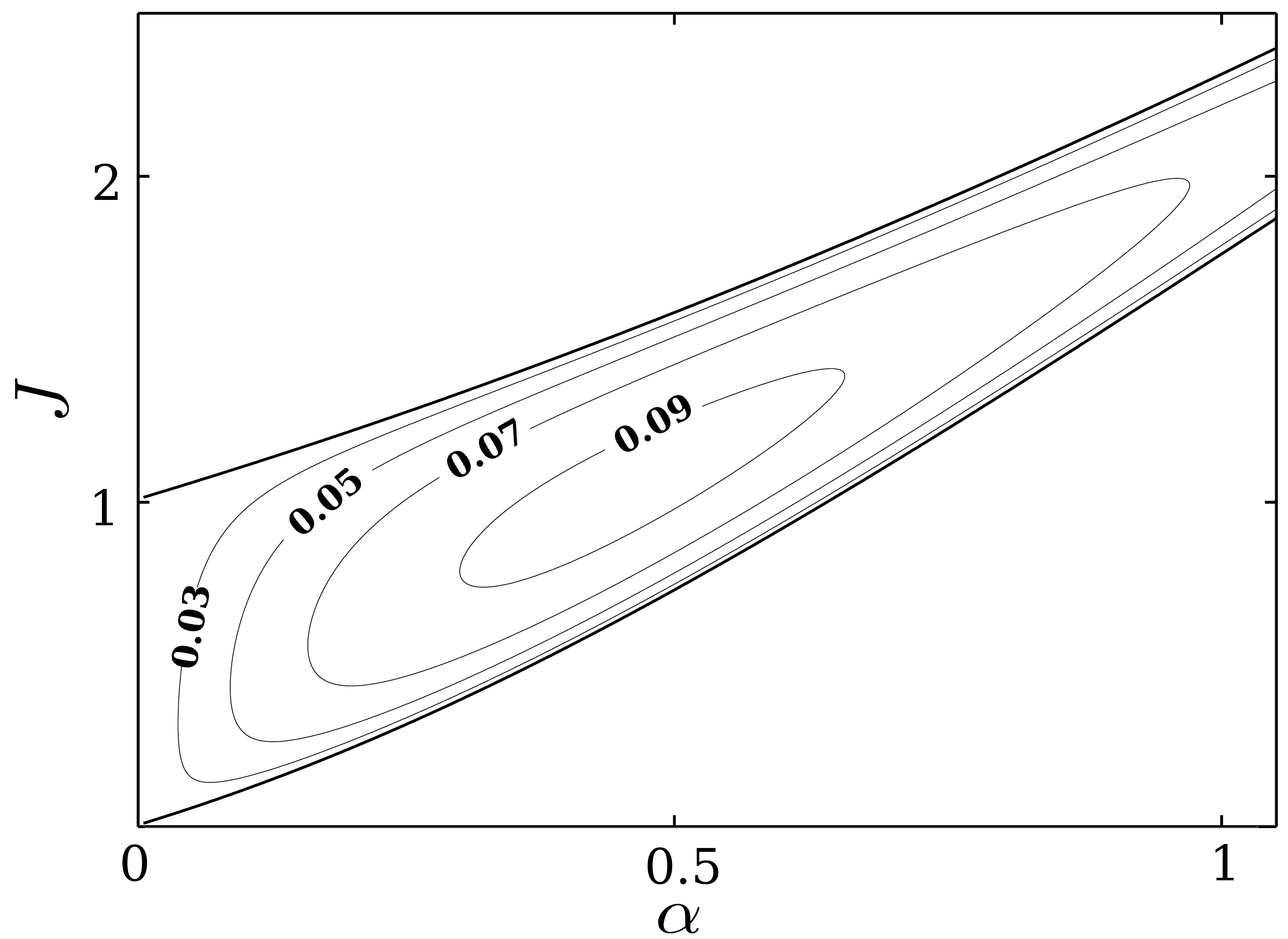
(b)

(c)

Figure 5: (a) The setting leading to the TC instability. The velocity and density profiles in (72) are shown on the left, while the gravity waves “G” are shown on the right. (b) Linear stability diagram of the TC instability. The contours represent the growth-rate. (c) Phase portrait of TC instability corresponding to an unstable combination of $\alpha$ and $J$ ($\alpha=0.2$ and $J=0.7264$)

Probably the only way to make sense of TC instability is through wave interactions, which has been described in Caulfield (1994) and Carpenter et al. (2013) using normal-mode theory. WIT provides the framework for studying non-modal TC instability. Substituting (19) in (30)-(33), and performing non-dimensionalization, we obtain

$$\gamma_{1}=\frac{J}{2R(1+c_{2})}e^{-2\alpha}\sin\Phi$$ (74)

$$c_{1}=1-\sqrt{\frac{J}{2\alpha}\left(1-\frac{\beta}{R}e^{-2\alpha}\cos\Phi\right)}$$ (75)

$$\gamma_{2}=\frac{JR}{2(1-c_{1})}e^{-2\alpha}\sin\Phi$$ (76)

$$c_{2}=-1+\sqrt{\frac{J}{2\alpha}\left(1-\frac{R}{\beta}e^{-2\alpha}\cos\Phi\right)}.$$ (77)

Here $\beta=\upomega_{2}/\upomega_{1}=(1-c_{1})/(1+c_{2})$, and by definition is a positive quantity. From (75) and (77) we construct a quadratic equation for $\beta$:

$$\beta^{2}+\beta e^{-2\alpha}\cos\Phi\left(\frac{1}{R}-R\right)-1=0.$$ (78)

Amongst the two roots, only the positive root is relevant. Equations (74)-(77) provide a non-modal description of TC instability. The equation-set is of coupled nature, and is therefore not homomorphic to (30)-(33). The non-linear dynamical system in this case is given by

$$\dot{R}=\frac{J}{2}\left(\frac{1}{1+c_{2}}-\frac{R^{2}}{1-c_{1}}\right)e^{-2\alpha}\sin\Phi$$ (79)

$$\dot{\Phi}=2\alpha-\sqrt{\frac{J\alpha}{2}\left(1-\frac{\beta}{R}e^{-2\alpha}\cos\Phi\right)}-\sqrt{\frac{J\alpha}{2}\left(1-\frac{R}{\beta}e^{-2\alpha}\cos\Phi\right)}.$$ (80)

At phase-locking $R=R_{NM}=\sqrt{\beta}$. Substituting this value in (78) gives $\beta=1$. Therefore $R_{NM}=1$ and $c_{1}=c_{2}=0$ at resonance, which implies that TC instability, like KH, also evolves into a stationary disturbances.

The phase portrait is shown in figure 5(c). The phase-shift $\Phi_{NM}$ is evaluated from (80):

$$\Phi_{NM}=\cos^{-1}\left[\left(1-\frac{2\alpha}{J}\right)e^{2\alpha}\right].$$ (81)

The N&S condition for TC instability is given by

$$-1\leq\left(1-\frac{2\alpha}{J}\right)e^{2\alpha}\leq 1\,\,\,\,\mathsf{\mathrm{implying}}\,\,\,\,\frac{2\alpha}{1+e^{-2\alpha}}\leq J\leq\frac{2\alpha}{1-e^{-2\alpha}}.$$ (82)

The latter result corroborates the classical normal-mode result given in (73).

Non-modal TC instability has also been studied by Rabinovich et al. (2011). In their paper the non-modal equation-set is given by (3.11a,b)-(3.12a,b), which is quite different from our equation-set (74)-(77). However, these two equation-sets should be identical since they are describing the same physical problem. Using the equation-set of Rabinovich et al. (2011) we obtained the following range of unstable wavenumbers: $2\alpha/\left(1+e^{-2\alpha}\right)^{2}\leq J\leq 2\alpha/\left(1-e^{-2\alpha}\right)^{2}$. This bound is different from the correct stability bound (73).

5.3 The Holmboe Instability

Let us consider the following velocity and density profiles

$$U(z)=\begin{cases}U_{1}&z\geq z_{1}\\ Sz&z\leq z_{1}\end{cases}\,\,\,\,\mathrm{and}\,\,\,\,\rho\left(z\right)=\begin{cases}\rho_{0}&z\geq z_{2}\\ \rho_{0}+\triangle\rho&z\leq z_{2}.\end{cases}$$ (83)

We nondimensionalize (83) exactly like the TC instability problem, which gives us the dimensionless velocity and density profiles:

$$U(z)=\begin{cases}1&z\geq 1\\ z&z\leq 1\end{cases}\,\,\,\,\mathrm{and}\,\,\,\,\rho\left(z\right)=\begin{cases}0&z\geq 0\\ 2&z\leq 0.\end{cases}$$ (84)

The vorticity interface at the top supports a vorticity wave, while the density interface at the bottom supports two gravity waves. The interaction between the left moving vorticity wave at the upper interface and the right moving gravity wave at the lower interface leads to an instability mechanism, known as the “Holmboe instability” (Note that the generation of ocean surface gravity waves by wind shear Miles (1957) can be viewed as “non-Boussinesq Holmboe instability”, and can therefore be interpreted using wave interactions.). The corresponding flow setting is shown in figure 6(a).

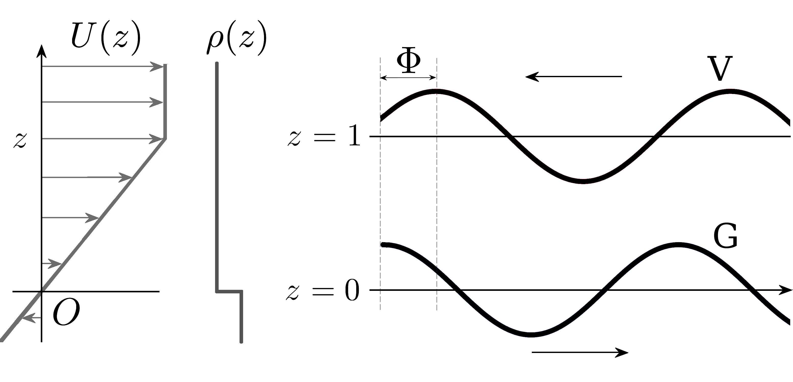
(a)

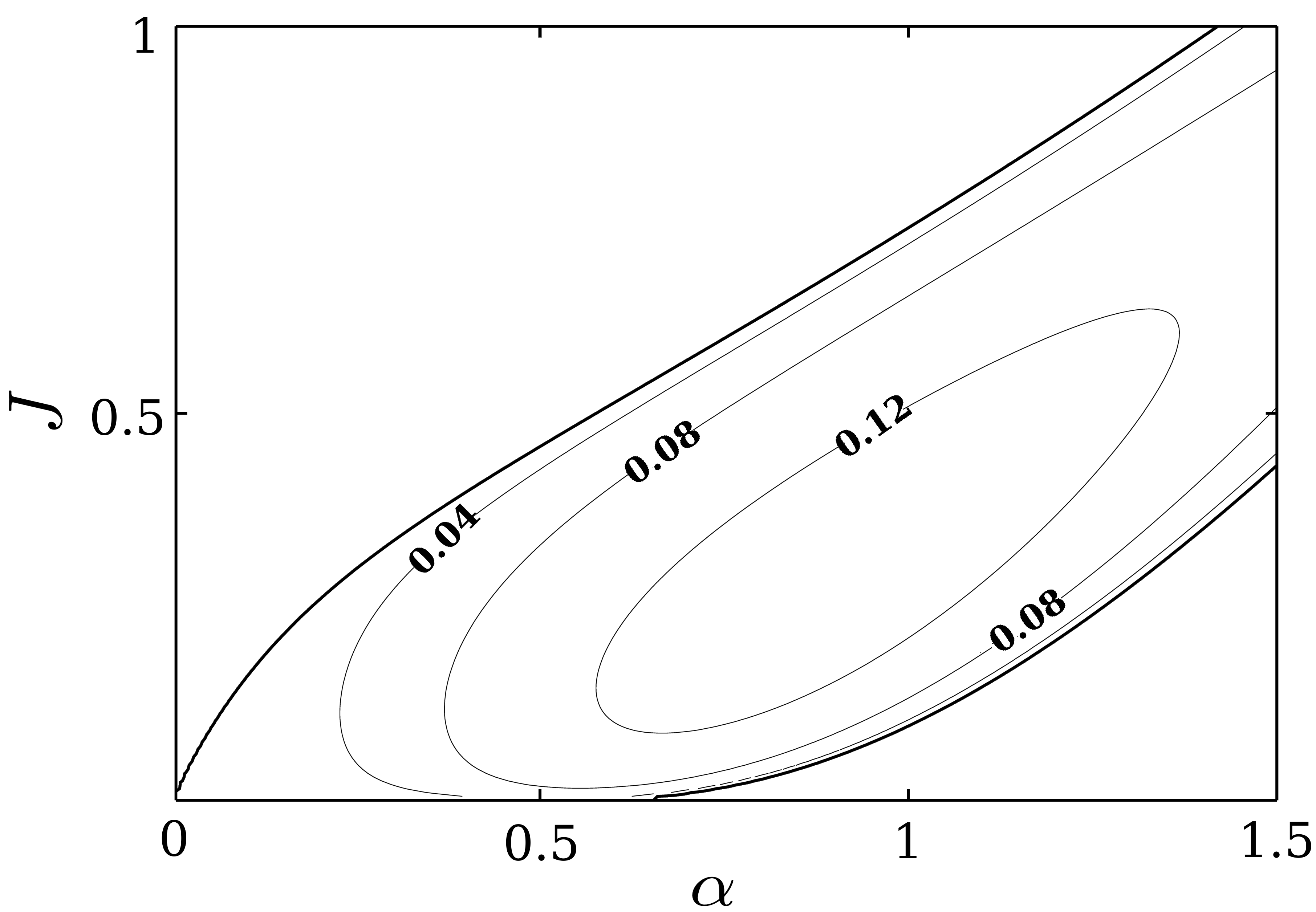
(b)

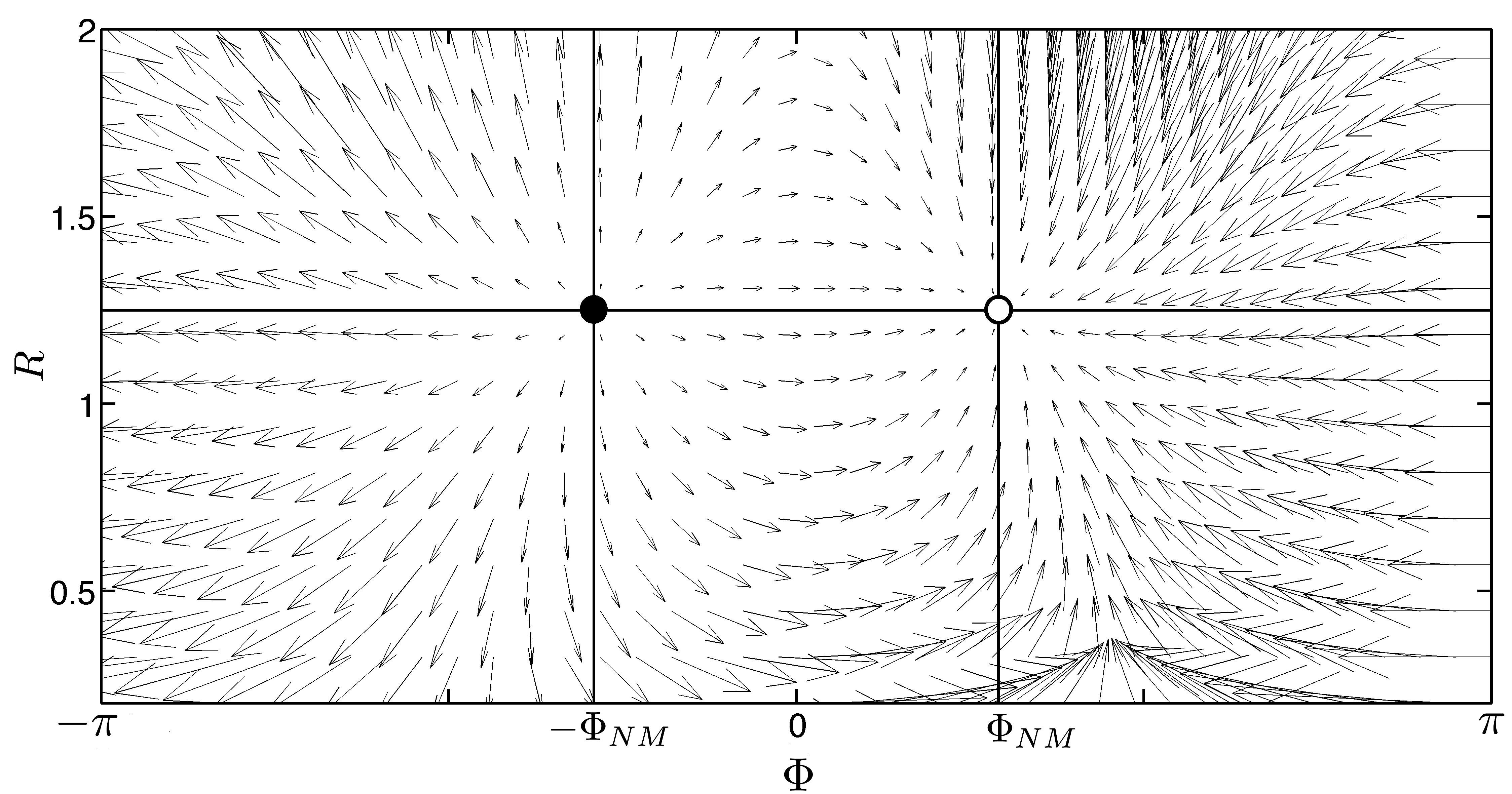
(c)

Figure 6: (a) The setting leading to the Holmboe instability. The velocity and density profiles in (84) are shown on the left, while the vorticity wave “V” and the gravity wave “G” are shown on the right. (b) Linear stability diagram; contours represent growth-rate. (c) Phase portrait corresponding to $\alpha=1$ and $J=0.5$.

Holmboe (1962) was the first to consider the instability mechanism resulting from the interaction between vorticity and gravity waves. Performing a normal-mode stability analysis, Holmboe discovered the existence of an unstable mode characterized by traveling waves. The profile used by Holmboe is more complicated than that which we are considering. Holmboe’s profile, which included multiple wave interactions, was substantially simplified by Baines & Mitsudera (1994) by introducing the profile in (84). Linear stability analysis shows that corresponding to each value of $J$, there exists a band of unstable wavenumbers, shown in figure 6(b). The stability boundary has been evaluated in Appendix B.

In order to understand the Holmboe instability in terms of WIT, we substitute (14) and (19) in (30)-(33). After non-dimensionalization, we obtain

$$\gamma_{1}=\frac{J}{Rc_{2}}e^{-\alpha}\sin\Phi$$ (85)

$$c_{1}=1-\frac{1}{\alpha}\left(\frac{1}{2}-\frac{J}{Rc_{2}}e^{-\alpha}\cos\Phi\right)$$ (86)

$$\gamma_{2}=\frac{R}{2}e^{-\alpha}\sin\Phi$$ (87)

$$c_{2}=\frac{1}{4\alpha}\left(-Re^{-\alpha}\cos\Phi+\sqrt{R^{2}e^{-2\alpha}\cos^{2}\Phi+16\alpha J}\right).$$ (88)

Like the TC instability case, the Holmboe equation-set is also of coupled nature, and is therefore not homomorphic to (30)-(33). The non-linear dynamical system is given by:

$$\dot{R}=\left(\frac{4\alpha J}{-Re^{-\alpha}\cos\Phi+\sqrt{R^{2}e^{-2\alpha}\cos^{2}\Phi+16\alpha J}}-\frac{R^{2}}{2}\right)e^{-\alpha}\sin\Phi$$ (89)

$$\dot{\Phi}=\alpha-\frac{1}{2}\left(1-Re^{-\alpha}\cos\Phi\right)+$$

$$\,\,\,\,\,\,\,\,\,\,\,\,\,\,\,\,\frac{4\alpha J}{-Re^{-\alpha}\cos\Phi+\sqrt{R^{2}e^{-2\alpha}\cos^{2}\Phi+16\alpha J}}\left(\frac{e^{-\alpha}\cos\Phi}{R}-1\right).$$ (90)

The equilibrium points of this system are $(R_{NM},\pm\Phi_{NM})$, where

$$R_{NM}=\sqrt{\frac{1-2\alpha+\sqrt{32\alpha J+\left(1-2\alpha\right)^{2}}}{2}}$$ (91)

$$\Phi_{NM}=\cos^{-1}\left[\left(\frac{R_{NM}^{2}+1-2\alpha}{2R_{NM}}\right)e^{\alpha}\right].$$ (92)

The N&S condition for Holmboe instability is found to be

$$-1\leq\left(\frac{R_{NM}^{2}+1-2\alpha}{2R_{NM}}\right)e^{\alpha}\leq 1.$$ (93)

This provides the range of $J$ leading to Holmboe instability, and is as follows:

$$\frac{1}{2A}\left(-B-\sqrt{B^{2}-4AC}\right)\leq J\leq\frac{1}{2A}\left(-B+\sqrt{B^{2}-4AC}\right),$$ (94)

where

$$A=16\alpha^{2}$$

$$B=-\alpha\left[8\left(2\alpha-1\right)^{2}+36\left(2\alpha-1\right)e^{-2\alpha}+27e^{-4\alpha}\right]$$

$$C=\left(2\alpha-1+e^{-2\alpha}\right)\left(2\alpha-1\right)^{3}.$$

Eq. (94) corroborates the normal-mode result given in Appendix B.

The phase portrait of Holmboe instability, corresponding to an unstable combination of $\alpha$ and $J$, is shown in figure 6(c). This phase portrait is slightly different from TC and KH instabilities, because $R_{NM}\neq 1$ in this case. Another feature of Holmboe instability is that, unlike TC and KH instabilities, its phase-speed is non-zero at the equilibrium condition. This phase-speed is found to be

$$c_{1}=c_{2}=\frac{2J}{R_{NM}^{2}}=\frac{4J}{1-2\alpha+\sqrt{32\alpha J+\left(1-2\alpha\right)^{2}}}.$$ (95)

In the limit of large $\alpha$ and $J$, the two phase-locked waves move with a speed of unity to the positive $x$ direction.

6 Conclusion

Shear instability plays a crucial role in atmospheric and oceanic flows. In the last 50 years, significant efforts have been made to develop a mechanistic understanding of shear instabilities. Using idealized velocity and density profiles, researchers have conjectured that the resonant interaction between two counter-propagating linear interfacial waves is the root cause behind exponentially growing instabilities in homogeneous and stratified shear layers. Support for this claim has been provided by considering interacting vorticity and gravity waves of the normal-mode form.

In this paper we investigated the wave interaction problem in a generalized sense. The governing equations (30)-(33) of hydrodynamic instability in idealized (broken-line profiles), homogeneous or density stratified, inviscid shear layers have been derived without imposing the wave type, or the normal-mode waveform. We refer to this equation-set as Wave Interaction Theory (WIT). Using WIT we showed in figures 2(a) and 2(b) that two counter-propagating linear interfacial waves, having arbitrary initial amplitudes and phases, eventually resonate (lock in phase and amplitude), provided they satisfy the N&S condition (39). In §4.1.1 we showed that the N&S condition is basically the criterion for normal-mode type instabilities. The waves which do not satisfy the N&S condition may exhibit non-normal instabilities, but will never resonate. In other words, such waves will never lock in phase and undergo exponential growth. These facts have been demonstrated in figures 3(c) and 3(d). We considered three classic examples of shear instabilities - Rayleigh/Kelvin-Helmholtz (KH), Taylor-Caulfield (TC) and Holmboe, and derived their discrete spectrum non-modal stability equations by modifying the basic WIT equations (30)-(33). These equations are respectively given by (62)-(65), (74)-(77) and (85)-(88). For each type of instability we validated the corresponding equation-set by showing that the N&S condition matches the predictions of the canonical normal-mode theory.

Although validation is an important first step for checking the non-modal equation-sets, the aim of this work is not proving well-known results using an alternative theory. The real strength of the non-modal formulation is in providing the opportunity to explore the transient dynamics. Non-orthogonal interaction between the two wave modes can lead to rapid transient growth. We show in figure 3(b) that depending on wavenumber and initial phase-shift, non-modal gain can exceed corresponding modal-gain by several orders of magnitude. This implies that the flow may become non-linear during the initial stages of flow development, leading to an early transition to turbulence. Instability has been observed for wavenumbers which are deemed stable by the normal-mode theory. All these facts are shown for the example of KH instability; see figures 3(a)-(d). In order to be able to study the transient dynamics of Holmboe and TC instabilities, the analysis in §4 needs to be modified in parts. This is because the equations developed in §4 are restricted to systems whose non-modal equation-sets are homomorphic to (30)-(33). Some examples of homomorphic equation-sets are: (62)-(65) representing KH instability, (14a)-(14d) of Heifetz, Bishop & Alpert (1999) representing barotropic shear instability, and (7a)-(7d) of Davies & Bishop (1994) representing baroclinic instability of the Eady model.

Another objective of our work is to provide an intuitive description of shear instabilities, and to find connection with other physical processes. How two waves can interact to produce instability has been discussed throughout the paper, and schematically represented in figure 1. We observed an analogy between WIT equations and that governing the synchronization of two coupled harmonic oscillators. On the basis of this analogy, we re-framed WIT as a non-linear dynamical system. The resonant configuration of the wave equations translated into a steady state configuration of the dynamical system. This dynamical system is of the source-sink type; the source and the sink nodes being the two equilibrium points. When interpreted in terms of canonical linear stability theory, the source and the sink nodes respectively correspond to the decaying and the growing normal-modes of the discrete spectrum. The analogous two coupled harmonic oscillator system exhibits two normal modes of vibration - the in-phase and the anti-phase synchronization modes. The growing normal-mode of WIT is analogous to the in-phase synchronization mode, while the decaying normal-mode is analogous to the anti-phase synchronization mode.

Although we studied WIT in the context of shear instabilities, the framework is actually derived from (26)-(29), and is therefore applicable to both sheared and unsheared flows, as well as co-propagating and counter-propagating waves. As an example, one can study the interaction between deep water surface gravity and internal gravity waves (which gives rise to barotropic and baroclinic modes of oscillations in lakes; see Kundu & Cohen (2004) Pg. 259-261). The framework can also be extended to the weakly non-linear regime to study multiple-wave interactions leading to resonant triads Wen (1995); Hill & Foda (1996); Jamali, Seymour & Lawrence (2003). WIT can also be applied to understand liquid-jet instability Jazayeri & Li (2000).

Finally we focus on the implications of using broken-line profiles of velocity and/or density. These idealizations have allowed us to concentrate only on the discrete spectrum dynamics and understand hydrodynamic instability in terms of interfacial wave interactions. Real profiles are always continuous, hence realistic analysis requires inclusion of the continuous spectrum. Using Green’s function, Heifetz & Methven (2005) have shown that the continuous spectrum dynamics in a smooth homogeneous shear layer can be understood in terms of infinite number of interacting vorticity (Rossby edge) waves. Harnik et al. (2008) used the same approach to understand the normal-mode continuous spectrum of smooth stratified shear layers. These studies indicate that the growth process is better understood through the “Orr mechanism” of shearing of waves Orr (1907); Heifetz & Methven (2005), than edge wave interactions. This implies that the intuition brought by WIT formulation may become less apparent in continuous systems. However the applicability of WIT in continuous systems can only be properly judged when the current version is modified to include the effects of a continuous spectrum. We speculate that the analogy between WIT and the synchronization of coupled harmonic oscillators can be exploited to obtain an intuitive understanding of continuous spectrum dynamics. Our speculation is based on the work of Balmforth & Sassi (2000), who studied the Kuramoto model in the continuous limit, and observed superficial similarities between oscillator synchronization and instabilities in ideal plasmas and inviscid fluids.

Appendix A Stokes’ theorem applied to a vorticity interface

Stokes’ theorem relates the surface integral of the curl of a vector (velocity in this case) field $\vec{u}$ over a surface $A$ to the line integral of the vector field over its boundary $\delta A$:

$$\oint_{\delta A}\vec{u}\cdot d\vec{l}=\iint_{A}\left(\nabla\times\vec{u}\right)\cdot d\vec{A}.$$ (96)

Holmboe (1962) used this theorem to relate the interfacial displacement $\eta_{i}$ with the difference in velocity perturbation ($u_{i}^{+}-u_{i}^{-}$) produced at a vorticity interface; see (12). This equation is referred to as “Eq. (3.2)” in his paper. However, the relevant steps required to derive this equation were not provided. In order to understand how (12) is obtained, we first graphically describe the problem in figure 7. The background velocity is such that the flow is irrotational when $z>z_{i}$, and has a constant vorticity, say $S$, when $z\leq z_{i}$. When the interface is disturbed by an infinitesimal displacement $\eta_{i}$ (solid black curve in figure 7), the velocity field also changes slightly - the perturbation velocity in the upper layer ($z>z_{i}$) becomes $u_{i}^{+}$ and that in the lower layer ($z\leq z_{i}$) becomes $u_{i}^{-}$.

Figure 7: Schematic of a vorticity interface - left half shows unperturbed velocity field, while the right half depicts infinitesimal interfacial displacement.

Let us consider a circuit A-B-C-D. Applying Stokes’ theorem, we obtain

$$(u_{i}^{+}-u_{i}^{-})\triangle x=S\cdot A,$$ (97)

where $A=\eta_{i}\cdot\triangle x$ is the area of A-B-C-D, and $S=\nabla\times\vec{u}$ is the vorticity in this area. Therefore we obtain

$$u_{i}^{+}-u_{i}^{-}=S\cdot\eta_{i},$$ (98)

which is basically (12).

Appendix B Normal mode form of Holmboe instability

Both interfaces in the Holmboe profile (84) individually satisfy the kinematic condition:

$$\frac{\partial\eta_{1}}{\partial t}=\frac{\partial}{\partial x}\left(e^{-\alpha}\psi_{2}+\frac{1-2\alpha}{2\alpha}\eta_{1}\right)$$ (99)

$$\frac{\partial\eta_{2}}{\partial t}=\frac{\partial}{\partial x}\left(\psi_{2}+\frac{e^{-\alpha}}{2\alpha}\eta_{1}\right),$$ (100)

where $\psi_{2}$ is the stream function perturbation at the lower interface. This interface being a density interface also satisfies the dynamic condition:

$$\frac{\partial\psi_{2}}{\partial x}=\frac{J}{\alpha}\frac{\partial\eta_{2}}{\partial x}.$$ (101)

We assume the perturbations to be of normal-mode form: $\eta_{1}=\Re\{\hat{\eta}_{1}e^{{\rm i}\alpha(x-ct)}\}$, $\eta_{2}=\Re\{\hat{\eta}_{2}e^{{\rm i}\alpha(x-ct)}\}$, and $\psi_{2}=\Re\{\hat{\psi}_{2}e^{{\rm i}\alpha(x-ct)}\}$. Here the wave speed $c$ is generally complex. Defining $\hat{\varsigma}=\left[\begin{array}[]{ccc}\hat{\psi}_{2}&\hat{\eta}_{2}&\hat{\eta}_{1}\end{array}\right]^{T}$, we obtain the following eigenvalue problem:

$$\left(M+cI\right)\hat{\varsigma}=0,$$ (102)

where

$$M=\left[\begin{array}[]{ccc}0&J/\alpha&0\\ 1&0&e^{-\alpha}/(2\alpha)\\ e^{-\alpha}&0&(1-2\alpha)/(2\alpha)\end{array}\right].$$ (103)

Eq. (102) generates the following characteristic polynomial:

$$c^{3}+\left(\frac{1-2\alpha}{2\alpha}\right)c^{2}-\frac{J}{\alpha}c-J\left(\frac{1-2\alpha}{2\alpha^{2}}\right)+J\frac{e^{-2\alpha}}{2\alpha^{2}}=0.$$ (104)

This equation produces complex conjugate roots only when the discriminant is negative. Since the presence of complex roots signify normal-mode instability, negative values of the discriminant is of our interest. The discriminant (D) in this case is given by:

$$D=16\alpha^{2}J^{2}-\alpha J\left[8\left(2\alpha-1\right)^{2}+36e^{-2\alpha}\left(2\alpha-1\right)+27e^{-4\alpha}\right]-\left(1-2\alpha\right)^{3}\left(2\alpha-1+e^{-2\alpha}\right).$$ (105)

Imposing the condition $D<0$, we find

$$\frac{1}{2A}\left(-B-\sqrt{B^{2}-4AC}\right)\leq J\leq\frac{1}{2A}\left(-B+\sqrt{B^{2}-4AC}\right),$$ (106)

where

$$A=16\alpha^{2}$$

$$B=-\alpha\left[8\left(2\alpha-1\right)^{2}+36\left(2\alpha-1\right)e^{-2\alpha}+27e^{-4\alpha}\right]$$

$$C=\left(2\alpha-1+e^{-2\alpha}\right)\left(2\alpha-1\right)^{3}.$$

Thus Holmboe instability occurs only when the condition in (106) is satisfied.

References

- Baines & Mitsudera (1994) Baines, P. G. & Mitsudera, H. 1994 On the mechanism of shear flow instabilities. J. Fluid Mech. 276, 327–342.
- Bakas & Ioannou (2011) Bakas, N. A. & Ioannou, P. J. 2009 Modal and nonmodal growths of inviscid planar perturbations in shear flows with a free surface. Phys. Fluids 21 (2), 024102.
- Balmforth & Sassi (2000) Balmforth, N. J. & Sassi, R. 2000 A shocking display of synchrony. Phys. D 143, 21–55.
- Bretherton (1966) Bretherton, F. P. 1966 Baroclinic instability and the short wavelength cut-off in terms of potential vorticity. Q. J. Roy. Meteor. Soc. 92 (393), 335–345.
- Cairns (1979) Cairns, R. A. 1979 The role of negative energy waves in some instabilities of parallel flows. J. Fluid Mech. 92, 1–14.
- Carpenter et al. (2013) Carpenter, J. R., Tedford, E. W., Heifetz, E. & Lawrence, G. A. 2013 Instability in stratified shear flow: Review of a physical interpretation based on interacting waves. Appl. Mech. Rev. 64 (6), 060801-17.
- Caulfield (1994) Caulfield, C. P. 1994 Multiple linear instability of layered stratified shear flow. J. Fluid Mech. 258, 255–285.
- Caulfield et al. (1995) Caulfield, C. P., Peltier, W. R., Yoshida, S. & Ohtani, M. 1995 An experimental investigation of the instability of a shear flow with multilayered density stratification. Phys. Fluids 7, 3028–3041.
- Constantinou & Ioannou (2011) Constantinou, N. C. & Ioannou, P. J. 2011 Optimal excitation of two dimensional Holmboe instabilities. Phys. Fluids 23 (7), 074102.
- Davies & Bishop (1994) Davies, H. C. & Bishop, C. H. 1994 Eady edge waves and rapid development. J. Atmos. Sci. 51 (13), 1930–1946.
- Drazin & Howard (1966) Drazin, P. G. & Howard, L. N. 1966 Hydrodynamic stability of parallel flow of inviscid fluid. 9, Academic Press.
- Drazin & Reid (2004) Drazin, P. G. & Reid, W. H. 2004 Hydrodynamic Stability, 2nd edn. Cambridge University Press.
- Farrell (1984) Farrell, B. 1984 Modal and non-modal baroclinic waves. J. Atmos. Sci. 41 (4), 668–673.
- Farrell & Ioannou (1996) Farrell, B. F. & Ioannou, P. J. 1996 Generalized stability theory. Part I: Autonomous operators. J. Atmos. Sci. 53 (14), 2025–2040.
- Goldstein (1931) Goldstein, S. 1931 On the stability of superposed streams of fluids of different densities. Proc. R. Soc. Lond. A 132, 524–548.
- Guha, Rahmani & Lawrence (2013) Guha, A., Rahmani, M. & Lawrence, G. A. 2013 Evolution of a barotropic shear layer into elliptical vortices. Phys. Rev. E 87, 013020.
- Harnik et al. (2008) Harnik, N., Heifetz, E., Umurhan, O. M. & Lott, F. 2008 A buoyancy-vorticity wave interaction approach to stratified shear flow. J. Atmos. Sci. 65 (8), 2615–2630.
- Heifetz, Bishop & Alpert (1999) Heifetz, E., Bishop, C. H. & Alpert, P. 1999 Counter-propagating Rossby waves in the barotropic Rayleigh model of shear instability. Q. J. R. Meteorol. Soc. 125 (560), 2835–2853.
- Heifetz et al. (2004) Heifetz, E., Bishop, C. H., Hoskins, B. J. & Methven, J. 2004 The counter-propagating rossby-wave perspective on baroclinic instability. I: Mathematical basis. Q. J. Roy. Meteor. Soc. 130 (596), 211–231.
- Heifetz & Methven (2005) Heifetz, E. & Methven, J. 2005 Relating optimal growth to counterpropagating Rossby waves in shear instability. Phys. Fluids 17 (6), 064107.
- Hill & Foda (1996) Hill, D. F. & Foda, M. A. 1996 Subharmonic resonance of short internal standing waves by progressive surface waves. J. Fluid Mech. 321, 217–234.
- Holmboe (1962) Holmboe, J. 1962 On the behavior of symmetric waves in stratified shear layers. Geofys. Publ. 24, 67–112.
- Hoskins, McIntyre & Robertson (1985) Hoskins, B. J., McIntyre, M. E. & Robertson, A. W. 1985 On the use and significance of isentropic potential vorticity maps. Q. J. Roy. Meteor. Soc. 111 (470), 877–946.
- Howard & Maslowe (1973) Howard, L. N. & Maslowe, S. A. 1973 Stability of stratified shear flows. Bound.-Layer Meteor. 4 (1–4), 511–523.
- Jamali, Seymour & Lawrence (2003) Jamali, M., Seymour, B. & Lawrence, G. A. 2003 Asymptotic analysis of a surface-interfacial wave interaction. Phys. Fluids 15 (1), 47–55.
- Jazayeri & Li (2000) Jazayeri,S. A. & Li, X. 2000 Nonlinear instability of plane liquid sheets. J. Fluid Mech. 406, 281–308.
- Kundu & Cohen (2004) Kundu, P. K. & Cohen, I. M. 2004 Fluid Mechanics. Elsevier.
- Lawrence, Browand & Redekopp (1991) Lawrence, G. A., Browand, F. K. & Redekopp, L. G. 1991 The stability of a sheared density interface. Phys. Fluids 3 (10), 2360–2370.
- Lee & Caulfield (2001) Lee, V. & Caulfield, C. P. 2001 Nonlinear evolution of a layered stratified shear flow. Dyn. Atmos. Oceans 34 (2), 103–124.
- Lindzen (1988) Lindzen, R. S. 1988 Instability of plane parallel shear flow (toward a mechanistic picture of how it works). Pure Appl. Geophys. 126 (1), 103–121.
- Miles (1957) Miles, J. W. 1957 On the generation of surface waves by shear flows. J. Fluid Mech. 3, 185–204.
- Orr (1907) Orr, W. M. F. 1907 Stability or instability of the steady motions of a perfect liquid and of a viscous liquid. Proc. Roy. Irish Acad. A (27), 9–138.
- Pikovsky, Rosenblum & Kurths (2001) Pikovsky, A., Rosenblum, M. G. & Kurths, J. 2001 Synchronization, A Universal Concept in Nonlinear Sciences, Cambridge University Press.
- Rayleigh (1880) Rayleigh, J. W. S. 1880 On the stability, or instability, of certain fluid motions. Proc. Lond. Math. Soc. 12, 57–70.
- Rabinovich et al. (2011) Rabinovich, A., Umurhan, O. M., Harnik, N., Lott, F. & Heifetz, E. 2011 Vorticity inversion and action-at-a-distance instability in stably stratified shear flow. J. Fluid Mech. 670, 301–325.
- Schmid & Henningson (2001) Schmid, P. J. & Henningson, D. S. 2001 Stability and transition in shear flows, 142. Springer Verlag.
- Sutherland (2010) Sutherland, B. R. 2010 Internal gravity waves, Cambridge University Press.
- Taylor (1931) Taylor, G. I. 1931 Effect of variation in density on the stability of superposed streams of fluid. Proc. R. Soc. Lond. A 132, 499–523.
- Tedford, Pieters & Lawrence (2009) Tedford, E. W., Pieters, R. & Lawrence, G. A. 2009 Symmetric Holmboe instabilities in a laboratory exchange flow. J. Fluid Mech. 636, 137–153.
- Tedford et al. (2009) Tedford, E. W., Carpenter, J.R., Pawlowicz, R., Pieters, R. & Lawrence, G. A. 2009 Observation and analysis of shear instability in the Fraser River estuary. J. Geophys. Res. 114, C11.
- Thorpe (1973) Thorpe, S. A. 1973 Experiments on instability and turbulence in a stratified shear flow. J. Fluid Mech. 61, 731–751.
- Trefethen et al. (1993) Trefethen, L. N., Trefethen, A. E., Reddy, S. C. & Driscoll, T. A. 1993 Hydrodynamic stability without eigenvalues. Science 261, 578–584.
- Turner (1973) Turner, J. S. 1973 Buoyancy Effects in Fluids, Cambridge University Press.
- Wen (1995) Wen, F. 1995 Resonant generation of internal waves on the soft sea bed by a surface water wave. Phys. Fluids 7 (8), 1915–1922.