A hydrodynamical model for the FERMI-LAT $\gamma$-ray light curve of Blazar PKS 1510-089

Abstract

A physical description of the formation and propagation of working surfaces inside the relativistic jet of the Blazar PKS 1510-089 are used to model its $\gamma$-ray variability light curve using FERMI-LAT data from 2008 to 2012. The physical model is based on conservation laws of mass and momentum at the working surface as explained by Mendoza et al. (2009). The hydrodynamical description of a working surface is parametrised by the initial velocity and mass injection rate at the base of the jet. We show that periodic variations on the injected velocity profiles are able to account for the observed luminosity, fixing model parameters such as mass ejection rates of the central engine injected at the base of the jet, oscillation frequencies of the flow and maximum Lorentz factors of the bulk flow during a particular burst.

1 Introduction

Among all types of AGN, Blazars (Blazar class is defined as radio loud sources conformed by the BL Lac objects and the Flat Spectrum Radio Quasars -FSRQ, see e.g. Fossati et al., 1997; Ghisellini et al., 1998, and references therein) represent the most energetic class. They are known to have the most powerful jets (e.g. Lister et al., 2009) and also show a highly variable Spectral Energy Distribution (SED) from the radio to the $\gamma$-rays wavelengths (see Abdo et al., 2010b; D’Ammando et al., 2011, and references therein).

The FSRQ PKS 1510-089 is known to be one of the most powerful astrophysical objects with a highly collimated relativistic jet that has shown apparent superluminal velocities between $20c$ to $46c$ and with a semi-angle aperture for the jet $\sim 0.2^{\circ}$ (Jorstad et al., 2005). Since the angle between the relativistic jet and the observer’s line of sight $\sim 1.4^{\circ}$ – $3^{\circ}$, the jet almost coincides with the observer’s line of sight (Homan et al., 2002; Marscher et al., 2010). PKS 1510-089 was one of the $\gamma$-ray sources detected by EGRET (Hartman et al., 1999). It has been monitored at high energies with AGILE (Pucella et al., 2008; D’Ammando et al., 2008; Lucarelli et al., 2012) and by FERMI-LAT and AGILE (Tramacere, 2008; Ciprini & Corbel, 2009; D’Ammando et al., 2009). It has also been studied with MAGIC and HESS (Cortina, 2012; Wagner et al., 2010). The most prominent outbursts displayed by PKS 1510-089 were reported by Kataoka et al. (2008), Ciprini & Corbel (2009) and Orienti et al. (2012). The high activity observed in this source, turns it into an ideal target for the physical study of its highly relativistic jet.

Precise models for the light curve (LC) produced by the outburst and flares from Blazars are not done using directly the data variations observed in different wavelengths. Instead, models are applied to explain the behaviour of the SED (e.g. Abdo et al., 2010b; D’Ammando et al., 2011). Direct understanding of the LC requires a precise knowledge of the hydrodynamical behaviour of the relativistic flow. Mendoza et al. (2009), hereafter M09, have constructed a hydrodynamical model of the motion of a working surface inside a relativistic jet which is able to fit the observed LCs of long Gamma-Ray Bursts (lGRB’s). Since the jets in Blazars are highly relativistic and their jet is nearly pointing towards the observer, similar to the jets observed in lGRB’s, the physical ingredients of both phenomena can be considered the same but occurring at different physical scales of energy, sizes, masses, accretion rates, etc. (cf. Mirabel & Rodriguez, 2002).

The Blazar PKS 1510-089 is of tremendous importance since it exhibits extreme relativistic motions. As such, its energy curve must present luminosity variations and periods of extreme activity displayed as outbursts that, when physically modelled, can yield a better understanding of the physical parameters associated to the mechanism producing the observed luminosity.

In this letter, we assume that the mechanism producing the observed LC in a typical lGRB is exactly the same that produces the variable LC of the Blazar PKS 1510-089. We thus apply the hydrodynamical jet model presented in M09 to the LC variations displayed by the Blazar PKS 1510-089 in the $\gamma$-ray domain, using public data obtained with the FERMI-LAT telescope.

The letter is organised as follows. In Section 2 we explain in general terms the data reduction process. In Section 3 we describe the characteristics of our hydrodynamic model. The fit done to the data with the hydrodynamic model is explained in Section 4. The results of our fits and the discussion of the main physical parameters obtained in the modelling are presented in Section 5. Throughout this letter we use a standard cosmology with $H_{0}=71\,\textrm{km}\,\textrm{s}^{-1}\,\textrm{Mpc}^{-1}$, $\Omega_{\textrm{m}}=0.27$ and $\Omega_{\lambda}=0.73$ (see e.g Kataoka et al., 2008, and references therein).

2 Fermi-LAT Data

The gamma-ray fluxes were obtained in the range of 0.2 to 300 GeV using the public database of FERMI-LAT from 2008 August 08 to 2012 May 28. The data were reduced with the FERMI science tool package (see e.g. Atwood et al., 2009) in the same energy range, taking into account the diffuse galactic background radiation, the instrument response matrix p7v6, and considering a zenith angle $<105^{\circ}$. We also calculated the active time of the detector and the PSF. The $\gamma$-ray LC was constructed modelling the flux with a power law of the form $\mathrm{d}N/\mathrm{d}E=N_{0}(E/E_{0})^{\gamma}$, with $\gamma=2-3$ in accordance with the results of Abdo et al. (2010a). The fluxes and errors obtained with this package are given in photons $\times$ cm^-2 s^-1. For further physical interpretation of the data, we have converted these fluxes and errors to MeV cm^-2 s^-1.

The photons considered for analysis were taken from a region centred on the coordinates of PKS 1510-089 with a radius of $15^{\circ}$. Figure 1 shows the $\gamma$-ray LC, with a bin size of 1 day. We chose these bins, since the errors are larger using shorter bin sizes, complicating the analysis of the data and because particular outbursts can be adequately resolved.

From Figure 1 it follows that the source displayed the historical maximum outburst in MJD 55851, corresponding to 2011 October 17 and reported by Hungwe et al. (2011). Another important outburst occurred in MJD 54899 (2009 March 9) and was observed with AGILE (D’Ammando et al., 2009). Several flares or outbursts can be observed in the LC. The most relevant events occurred in MJD 54717 (2008 September 8), MJD 54843 (2009 January 12), MJD 55200 (2010 January 4, Benítez et al., 2011), MJD 55730 (2011 June 18), and MJD 55954 (2012 January 28). This last event was also observed by AGILE (Verrecchia et al., 2012) and MAGIC (Cortina, 2012). Note that Marscher et al. (2010) reports extra flares $<200\text{MeV}$ during the period 54850 - 54950 MJD, which are not seen in our $>200\text{MeV}$ selection.

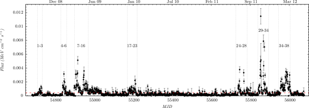
Figure 1: Fermi-LAT light curve of Blazar PKS 1510-089 (from 0.2 to 300 GeV) obtained from 2008 August to 2012 May. The outburst identification number (ID#) labelled in the figure stands for the different flares selected in our work (see text). The 3$\sigma$ noise level is represented by the red horizontal dashed line.

3 A hydrodynamical model for the Light Curve of PKS 1510-089

The formation of internal shock waves on a relativistic jet are commonly explained by different mechanisms, such as the interaction of the jet with inhomogeneities of the surrounding medium, the bending of jets and time fluctuations in the parameters of the ejection (see e.g. Rees & Meszaros 1994; Mendoza & Longair 2002; Jamil et al. 2008; Mendoza et al. 2009). In particular, the model by M09 is a hydrodynamical description that can be applied to shock waves inside relativistic jets. This semi-analytical model describes the formation of a working surface inside a hydrodynamical jet due to periodic variations of the injected flow. When fast flow overtakes slow flow, an initial discontinuity is formed and a working surface (two shock waves separated by a contact discontinuity) is produced. The working surface travels along the jet and radiates away kinetic energy. The article by M09 assumed that the efficiency converting factor is $\sim 1$ and that it is mostly emitted in the $\gamma$-ray band. As explained in Section 1, the Blazar PKS 1510-089 behaves as an scaled typical lGRB and as such, the hypothesis used by M09 can be extended to this particular object. As we will discuss in section 5, this assumption is coherent with the physical properties found from the model. Following M09, we assume that flow is injected at the base of the jet with a periodic velocity given by

$$v(\tau)=v_{0}+c\eta^{2}\sin\omega\tau,$$ (1)

where $\tau$ is the time in the rest frame of the source, the velocity $v_{0}$ is the “background” bulk velocity of the flow inside the jet, and $\omega$ is the oscillation frequency. The positive constant parameter $\eta^{2}$ is chosen in such a way that oscillations of the flow are small so that the bulk velocity $v(\tau)$ of the flow does not exceed the velocity of light $c$. The mass ejection rate $\dot{m}(\tau)$ from the central engine which is injected at the base of the jet is assumed constant through a particular outburst event, but is allowed to vary from one outburst to another. The radiated energy of the flow as a function of time is calculated as the difference between the total energy $E_{0}$ injected at the base of the jet and the kinetic energy inside the working surface $E_{\textrm{ws}}$. The luminosity $L$ is thus calculated as the derivative of this radiated energy with respect to time. As described by M09, there are two ways of calculating this luminosity curve. The first method consisted in a semi-analytical procedure and the second is performed with a full hydrodynamical numerical model. The authors showed that the semi-analytical model is in good agreement with the full numerical simulation, and as such we model the LC of PKS 1510-089 using their semi-analytical approach.

The semi-analytical approach is based on the assumption that equation (1) is valid and as such, one needs to know (or find through fits to observational data) the values of $v_{0}$, $\eta^{2}$, $\omega$ and $\dot{m}$. Furthermore, the mass ejection rate $\dot{m}$ enters in the description of the problem through the luminosity relation: $L\propto\dot{m}c^{2}$. The average bulk velocity $v_{0}$ must come from observational data (for this particular source D’Ammando et al., 2008, reports a value $\Gamma(v_{0})=18$). With this, the model is left with three free parameters: $\eta^{2}$, $\dot{m}$, and $\omega$, which can be fixed by fitting the best theoretical LC to the observational data.

4 Modelling the $\gamma$-ray Light Curve

To model the LC of Figure 1, we have selected the most conspicuous flares. The criterion used consists of selecting only those flares that are beyond $3\sigma$ noise level according to the errors shown in the LC. By doing so, it turns out that 38 relevant peaks were chosen for our fitting.

As explained in section 3, the model has four free parameters. The velocity parameter $v_{0}$ for this particular object is such that its Lorentz factor is $\Gamma(v_{0})=18$. To calculate the measured luminosity $L$ from the observed flux $F$, we multiply the observed flux $F$ by (Dermer, 1995; Dermer & Menon, 2009; Longair, 2011; Ghisellini et al., 1993): $4\pi D_{L}^{2}\delta^{-p}$ where the relativistic beaming $\delta:=1/\Gamma(v_{0})\left(1-\left(v_{0}/c\right)\cos\theta\right)\sim 18$, for a luminosity distance $D_{L}$, which for this particular case is $D_{L}=1919\,\textrm{Mpc}$ and the angle $\theta\sim 1.4^{\circ}-3^{\circ}$ is the angle between the jet and the observer’s line of sight (cf. Section 1). We have selected a beaming index $p=3$ in accordance with the results of Wu et al. (2011) for Blazars and lGRB’s.

The model presented by M09 is such that the theoretical luminosity and time are presented in a very particular system of units. To fit the best theoretical LC to the data, one needs to have a common system of units. To achieve this, we have normalised the “measured” Luminosity to its peak and the measured time to the FWHM of the measured LC. In order to compare with the theoretical model, the theoretical LC is also normalised to its peak and the time is normalised to the FWHM of the theoretical luminosity curve. Once both theoretical and measured LCs are in this common dimensionless system of units, this procedure allows us to fit the best theoretical LC by performing a $\chi^{2}$ statistical test to find the optimal parameter $\eta^{2}$. Note that in this normalised system of units, the model only depends on one free parameter: $\eta$. Once the value of $\eta$ is found, we can rescale back to physical units and in such a rescaling the parameters $\dot{m}$ and $\omega$ are obtained, since according to M09, $L\propto\dot{m}c^{2}$ and $t\propto\omega^{-1}$. The luminosity fits are then transformed to the observed flux dividing them by $4\pi D_{L}/\delta^{3+\alpha}$. The results of these fits are shown in Figure 2. The obtained values of the physical parameters of the model for each particular modelled outburst are presented in Table 1.

There are a certain subclass of outbursts that we do not model. These outbursts, labelled 8, 10, 20, 27 and 32 in Figure 1, do not have enough data to allow us an accurate modelling. The outburst labelled 11 seems to have a fall that develops into a constant value before reaching an expected minimum and no data points further, so it seems incomplete. Outburst 14 has huge errors and the $\chi^{2}$ statistical test does not converge. Outbursts 34 and 35 have large errors which also makes the modelling not accurate.

Date	ID	MJD	$\eta^{2}/c$	$\Gamma_{\text{max}}$	$\omega^{-1}$	$\dot{m}$
	$\#$	+54000	$10^{-3}$		$10^{3}\textrm{s}$	$10^{-3}\textrm{M}_{\odot}/\textrm{yr}$
08 Sep	1	$722.66$	$1.500$	$106$	$1.05$	$2.16$
08 Sep	2	$728.66$	$1.520$	$143$	$0.50$	$2.87$
08 Sep	3	$731.66$	$1.510$	$120$	$0.41$	$2.37$
09 Jan	5	$849.66$	$1.501$	$107$	$0.34$	$4.18$
09 Jan	6	$855.66$	$1.533$	$209$	$1.49$	$2.80$
09 Mar	7	$899.66$	$1.330$	$48$	$0.94$	$3.04$
09 Mar	9	$908.66$	$1.460$	$76$	$0.37$	$6.61$
09 Apr	12	$925.66$	$1.430$	$66$	$1.27$	$2.60$
09 Apr	13	$948.66$	$1.515$	$130$	$1.22$	$7.67$
09 May	15	$957.66$	$1.300$	$45$	$0.88$	$3.85$
09 May	16	$967.66$	$1.523$	$152$	$1.05$	$3.38$
09 Dic	17	$1182.66$	$1.534$	$219$	$2.60$	$2.40$
09 Dic	18	$1186.66$	$1.400$	$58$	$0.39$	$2.06$
09 Dic	19	$1191.66$	$1.488$	$94$	$1.24$	$2.84$
10 Jan	21	$1205.66$	$1.510$	$120$	$1.04$	$2.23$
10 Jan	22	$1209.66$	$1.493$	$98$	$0.95$	$4.76$
10 Mar	23	$1274.66$	$1.430$	$66$	$0.68$	$2.99$
11 Jun	24	$1739.66$	$1.460$	$76$	$0.74$	$3.16$
11 Jul	25	$1745.66$	$1.527$	$169$	$0.81$	$8.09$
11 Jul	26	$1766.66$	$1.469$	$81$	$0.36$	$7.13$
11 Aug	28	$1783.66$	$1.380$	$55$	$0.41$	$2.40$
11 Oct	29	$1848.66$	$1.460$	$76$	$0.67$	$3.30$
11 Oct	30	$1853.66$	$1.541$	$383$	$1.32$	$24.52$
11 Nov	31	$1867.66$	$1.522$	$149$	$0.57$	$16.83$
11 Nov	33	$1875.66$	$1.531$	$193$	$0.88$	$6.37$
12 Feb	36	$1972.66$	$1.220$	$39$	$0.66$	$3.55$
12 Mar	37	$1982.66$	$1.350$	$50$	$2.03$	$7.48$

Table 1: Different physical quantities obtained for the outbursts modelled in this work. The background Lorentz factor of the bulk velocity of the flow was assumed to be $18$. The first three columns from left to right are the date, numeric identification of the outburst (ID #) and the date corresponding to the maximum luminosity for a particular outburst. Columns four and six are the obtained values for the parameters $\eta^{2}$ (measured in units of the speed of light $c$) and the inverse frequency $\omega^{-1}$ relevant to the particular variational model of equation (1). Column five corresponds to the maximum upper limit of the Lorentz factor of the flow for each particular outburst. The minimum Lorentz factor of the flow for all outbursts is $\sim 12-13$. Column seven represents the mass injection rate $\dot{m}$ of the flow at the base of the jet. The values of all inferred parameters are accurate to within 10%.

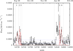
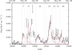
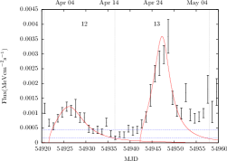
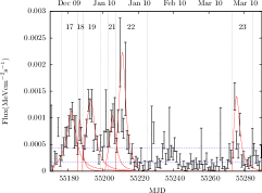
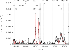
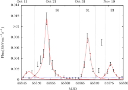
Figure 2: In each panel, the continuous red curve represents the fitting done to the light curve of PKS 1580-089 with the semi-analytical model of internal shock waves (working surfaces) by Mendoza et al. (2009). Blue horizontal dotted-lines in all panels show the $1~{}\sigma$ and $3~{}\sigma$ noise levels. Top-left panel shows variations from 2008 September to 2009 February. Top-right shows variations from 2009 February to 2009 May. The central left-panel shows a zoom of the peaks 12 and 13. The central right-panel shows a few outbursts observed from 2009 December to 2010 March. Bottom left-panel shows recent variations occurred from 2011 July to 2012 March. Finally, bottom-right panel shows a zoom of the prominent October 2011 outburst. This outburst is $\sim$ three times more luminous than the one observed in 2009 March. Up to now, this is the most violent outburst observed in the $\gamma$-ray waveband by FERMI.

5 Discussion

We have modelled the LC of Blazar PKS 1510-089 for almost 4 years using the hydrodynamical model of M09. The modelling was performed by assuming a periodic velocity injection mechanism at the base of the relativistic jet that leads to the formation of a working surface and is capable of loosing energy as it travels along the jet. As explained in section 3, the model by M09 was constructed to deal with LCs of lGRB. However, the Blazar PKS 1510-089 has many physical characteristics to be considered a geometrical large scaled version of a lGRB since it has a highly relativistic jet that points towards the observer. The results presented in Table 1 show high upper limits for the bulk Lorentz factors achieved with oscillations of the flow, that reach values as large as $\lesssim 380$ for one particular event. These inferred huge Lorentz factors in the bulk velocity oscillation of this Blazar show another close similarity with lGRB’s.

The range of parameters as presented in Table 1, i.e. $\dot{m}\sim\left(2-25\right)\times 10^{-3}\textrm{M}_{\odot}\textrm{yr}^{-1}$, $\omega^{-1}\sim\left(0.3-2.6\right)\times 10^{3}\,\textrm{s}$ and variations of the Lorentz factor $\Gamma\sim 10-380$, denote a scaling between the lGRB counterparts found in M09 for which $\dot{m}\sim 10^{-1}-10^{-2}\textrm{M}_{\odot}\textrm{s}^{-1}$, $\omega^{-1}\sim\ 10\textrm{s}$ and $\Gamma\sim 50-500$. Note that the maximum and minimum values of the Lorentz factor for a particular outburst take into account the observational errors of the LC. The real value lies in between those calculated ranges. The inferred high relativistic Lorentz factors associated to the motion of the bulk velocity of the flow inside the jet of PKS 1510-089 makes it an ideal candidate for the application of the hydrodynamical model of M09. This is why that physical model can be applied naturally to lGRB and in this particular case to the extreme relativistic motion of the jet in the Blazar PKS 1510-089. The energy released in each outburst can be calculated by taking the integral of the luminosity with respect to time, which occurs typically over periods of a few days. The value of this released energy is $\sim 10^{39}$ – $10^{40}$ J, which shows the tremendous energy released by each individual outburst. This energy is to be compared with the energy released in about $10~{}\text{s}$ by a lGRB which is $\sim 10^{44}~{}\text{J}$.

The most energetic burst, labelled 30, inyected at the base of the jet a total mass $m=\dot{m}\Delta t\sim 10^{-3}\,M_{\odot}$ while the burst lasted $\Delta t\sim 15\text{days}$. Analysis of all bursts shows that the ejected mass interval is $10^{-5}M_{\odot}\lesssim m\lesssim 10^{-3}M_{\odot}$, for a time duration range $4\text{days}\lesssim\Delta t\lesssim 30\text{days}$.

The variations of the injected flow at the base of the jet cause the formation of working surfaces that produce bursts of $\gamma$-rays in the structure of the jet. The physical mechanism producing the oscillations of the input flow, which allows fast fluid to overtake the slow one, leading to the formation of working surfaces, is beyond the scope of this letter. However, steady flow deviations and oscillations in such complicated phenomena are expected since the accretion-ejection mechanism associated to a particular object is not necessarily expected to be of constant velocity and mass accretion-ejection rates.

It is important to note that the assumption of seeing a Blazar as a scaled version of a lGRB is not new. In an early attempt for finding a unified model of jet and central-engine power, Mirabel & Rodriguez (2002) made this identification. The more relativistic a Blazar jet is, the more it will resemble a lGRB. The idea of having a unified physical model for all types of astrophysical jets was first suggested by the pioneering works for the astrophysical scaling laws of black holes by Sams et al. (1996) and Rees (1998). The work presented in this letter further strengths arguments about a unified picture of all astrophysical relativistic jets.

PKS 1510-089 resulted to be an ideal target to test the model by M09 since it closely resembles a lGRB in some of its outbursts. Future tests of the model have to be done with a wide variety of Light Curves from a large collection of Blazars and micro-quasars.

6 ACKNOWLEDGMENTS

We thank the anonymous referee for his valuable comments who helped us to produce a much improved version of our letter. This work was supported by three DGAPA-UNAM grants (PAPIIT IN116210-3, IN116211-3, IN111513-3). JIC acknowledges support given by IAUNAM as a visiting researcher. JIC, YUC, EB, SM, DH and MS thank support granted by CONACyT: 50102, 210965, 13654, 26344, 8366, 177304. The authors acknowledge the use of the FERMI-LAT publicly available data as well as the public data reduction software.

References

- Abdo et al. (2010a) Abdo A. A. et al., 2010a, ApJ, 721, 1425
- Abdo et al. (2010b) Abdo A. A. et al., 2010b, ApJ, 716, 30
- Atwood et al. (2009) Atwood W. B., et al., 2009, ApJ, 697, 1071
- Benítez et al. (2011) Benítez E. et al., 2011, in Revista Mexicana de Astronomia y Astrofisica Conference Series. pp 44–45
- Ciprini & Corbel (2009) Ciprini S., Corbel S., 2009, The Astronomer’s Telegram, 1897, 1
- Cortina (2012) Cortina J., 2012, The Astronomer’s Telegram, 3965, 1
- D’Ammando et al. (2008) D’Ammando F., et al., 2008, The Astronomer’s Telegram, 1436, 1
- D’Ammando et al. (2009) D’Ammando F., et al., 2009, Astronomy and Astrophysics, 508, 181
- D’Ammando et al. (2011) D’Ammando F., et al., 2011, Astronomy and Astrophysics, 529, A145
- Dermer (1995) Dermer C. D., 1995, ApJL, 446, L63
- Dermer & Menon (2009) Dermer C. D., Menon G., 2009, High Energy Radiation from Black Holes: Gamma Rays, Cosmic Rays, and Neutrinos
- Fossati et al. (1997) Fossati G., Celotti A., Ghisellini G., Maraschi L., 1997, in Ostrowski M., Sikora M., Madejski G., Begelman M., eds, Relativistic Jets in AGNs. pp 245–248
- Ghisellini et al. (1998) Ghisellini G., Celotti A., Fossati G., Maraschi L., Comastri A., 1998, MNRAS, 301, 451
- Ghisellini et al. (1993) Ghisellini G., Padovani P., Celotti A., Maraschi L., 1993, ApJ, 407, 65
- Hartman et al. (1999) Hartman R. C. et al., 1999, ApJS, 123, 79
- Homan et al. (2002) Homan D. C., Wardle J. F. C., Cheung C. C., Roberts D. H., Attridge J. M., 2002, ApJ, 580, 742
- Hungwe et al. (2011) Hungwe F., Dutka M., Ojha R., 2011, The Astronomer’s Telegram, 3694, 1
- Jamil et al. (2008) Jamil O., Fender R. P., Kaiser C. R., 2008, in Microquasars and Beyond.
- Jorstad et al. (2005) Jorstad S. G., et al., 2005, Astronomical Journal, 130, 1418
- Kataoka et al. (2008) Kataoka J., Madejski G., et al., 2008, ApJ, 672, 787
- Lister et al. (2009) Lister M. L., et al., 2009, ApJL, 696, L22
- Longair (2011) Longair M. S., 2011, High Energy Astrophysics
- Lucarelli et al. (2012) Lucarelli F. et al., 2012, The Astronomer’s Telegram, 3934, 1
- Marscher et al. (2010) Marscher A. P., et al., 2010, ApJL, 710, L126
- Mendoza et al. (2009) Mendoza S., Hidalgo J. C., Olvera D., Cabrera J. I., 2009, MNRAS, 395, 1403
- Mendoza & Longair (2002) Mendoza S., Longair M. S., 2002, MNRAS, 331, 323
- Mirabel & Rodriguez (2002) Mirabel I. F., Rodriguez L. F., 2002, Sky and Telescope, 103, 050000
- Orienti et al. (2012) Orienti M. et al., 2012, ArXiv e-prints
- Pucella et al. (2008) Pucella G. et al., 2008, Astronomy and Astrophysics, 491, L21
- Rees (1998) Rees M. J., 1998, in Black Holes and Relativistic Stars. pp 79–101
- Rees & Meszaros (1994) Rees M. J., Meszaros P., 1994, ApJL, 430, L93
- Sams et al. (1996) Sams B. J., Eckart A., Sunyaev R., 1996, Nature, 382, 47
- Tramacere (2008) Tramacere A., 2008, The Astronomer’s Telegram, 1743, 1
- Verrecchia et al. (2012) Verrecchia F., et al., 2012, The Astronomer’s Telegram, 3907, 1
- Wagner et al. (2010) Wagner S. J., Behera B., H.E.S.S. Collaboration 2010, in AAS/High Energy Astrophysics Division #11. p. 660
- Wu et al. (2011) Wu Q., Zou Y.-C., Cao X., Wang D.-X., Chen L., 2011, ApJL, 740, L21