The entropy and reversibility of cellular automata on Cayley tree

Abstract.

In this paper, we study linear cellular automata (CAs) on Cayley tree of order 2 over the field $\mathbb{F}_{p}$ (the set of prime numbers modulo $p$). We construct the rule matrix corresponding to finite cellular automata on Cayley tree. Further, we analyze the reversibility problem of this cellular automata for some given values of $a,b,c,d\in\mathbb{F}_{p}\setminus\{0\}$ and the levels $n$ of Cayley tree. We compute the measure-theoretical entropy of the cellular automata which we define on Cayley tree. We show that for CAs on Cayley tree the measure entropy with respect to uniform Bernoulli measure is infinity.

Mathematics Subject Classification: 37A15, 37B40.
Key words: Reversible Cellular Automata, Cayley tree, null boundary condition, Bernoulli measure, entropy.

1. Introduction

A cellular automaton (plural cellular automata, shortly CA) has been studied and applied as a discrete model in many areas of science. Cellular automata (CAs) have very rich computational properties and provide different models in computation. CAs were first used for modeling various physical and biological processes and especially in computer science. Recently, CAs have been widely investigated in many disciplines with different purposes such as simulation of natural phenomena, pseudo-random number generation, image processing, analysis of a universal model of computations, coding theory, cryptography, ergodic theory ([1, 4, 5, 6, 7, 8]).

Most of the studies and applications for CA is extensively done for one-dimensional (1-D) CA. ”The Game of Life” developed by John H. Conway in the 1960 s is an example of a two-dimensional (2-D) CA. John von Neumann in the late 40’s and early 50’s studied CA as a self-reproducing simple organisms [9]. 2-D CA with von Neumann neighborhood has found many applications and been explored in the literature [10]. Nowadays, 2-D CAs have attracted much of the interest. Some basic and precise mathematical models using matrix algebra built on field $\mathbb{Z}_{2}$ were reported for characterizing the behavior of two-dimensional nearest neighborhood linear CAs with null or periodic boundary conditions [4, 5, 6, 8, 10].

The reversibility problem of some special classes of 1-D CAs reflective and periodic boundary conditions has been studied with the help of matrix algebra approach by several researchers [11, 12]. In [3], we have defined a family of one-dimensional finite linear cellular automata with reflective boundary condition over the field $\mathbb{Z}_{p}$. In [32], we investigated 2D finite CA with a von Neumann neighborhood under periodic, adiabatic or reflexive boundaries conditions over the ternary field the field $\mathbb{Z}_{3}$, which can be considered as a three-state case. The application of linear rules on image matrix is demonstrated which forms the basis of self-replicating and self-similar patterns in image processing [32, 34, 35, 36]. Particularly the rules are used for image multiplication of one image into several replicating or similar images. In [33], we investigated error correcting codes via reversible cellular automata over finite fields. In this paper, we start with linear cellular automata (CA) in relation to a basic mathematical structure on regular Cayley tree of order 2. Recently, we have investigated the reversibility problem of multidimensional linear cellular automata under certain boundary conditions (null, periodic, reflective) on some lattices; however, we have not obtained exact algorithms for determining whether a multidimensional linear cellular automaton is reversible [3, 11, 12, 18, 33, 39, 40].

In Ref. [14], Fici and Fiorenzi have a first attempt to study topological properties of CA on the full tree shift $A^{\sum^{*}}$, where $\sum^{*}$ is the free monoid of finite rank $|\sum|$. In this case, the Cayley graph of $\sum^{*}$ is a regular $|\sum|$-ary rooted tree. Fici and Fiorenzi [14] have studied cellular automata defined on the full $k$-ary tree shift (for $k\geq 2$). In this paper, we study cellular automata on regular Cayley tree of order 2.

Several notions of the entropy of measure-preserving transformation on probability space in ergodic theory have been investigated [2, 38]. The notion of entropy, both topological and measure-theoretical is one of the fundamental invariants in ergodic theory. In the last years, a lot of works have been devoted to this subject [1, 2, 15, 16, 17]. Recall that by the Variational Principle the topological entropy is the supremum of the entropies of invariant measures. In [1], the author has shown that the uniform Bernoulli measure is a measure of maximal entropy for some 1-D LCAs. Morris and Ward [19] proved that an ergodic additive CA in two dimensions has infinite topological entropy (see [20] for details). Recently, Blanchard and Tisseur [21] have introduced the entropy rate of multidimensional CAs and proved several results that show that entropy rate of 2-D CA preserve similar properties of the entropy of 1-D CA.

In this present paper, firstly we define cellular automata on Cayley tree (or Bethe lattice) of order 2. This generalizes the case of one-sided CA (where order of the Cayley tree is one). We construct a transition rule matrix corresponding to finite cellular automata on Cayley tree by using matrix algebra built on the field $\mathbb{Z}_{p}$ (the set of prime numbers modulo $p$). Further, we discuss the reversibility problem of this cellular automata. Lastly, we study the measure theoretical entropy of the CAs on Cayley tree. We show that for CAs on Cayley tree the measure entropy with respect to uniform Bernoulli measure is infinity.

2. Finite CA over Cayley tree

Let $\mathbb{F}_{p}=\{0,1,\ldots,p-1\}$ $(p\geq 2)$ be the field of the prime numbers modulo $p$ ($\mathbb{F}_{p}$ is called a state space). The Cayley tree $\Gamma^{k}$ of order $k\geq 1$ is an infinite tree, i.e., a graph without cycles, from each vertex of which exactly $k+1$ edges issue. Let $\Gamma^{k}=(V,L,i)$, where $V$ is the set of vertices of $\Gamma^{k}$, $L$ is the set of edges of $\Gamma^{k}$ and $i$ is the incidence function associating each edge $\ell\in L$ with its end points $x,y\in V.$ A configuration $\sigma$ on $V$ is defined as a function $x\in V\to\sigma(x)\in\mathbb{F}_{p}$; in a similar manner one defines configurations $\sigma_{n}$ and $\omega$ on $V_{n}$ and $W_{n}$, respectively. The set of all configurations on $V$ (resp. $V_{n}$, $W_{n}$) coincides with $\Omega=\mathbb{F}_{p}^{V}$ (resp. $\Omega_{V_{n}}=\mathbb{F}_{p}^{V_{n}},\ \ \Omega_{W_{n}}=\mathbb{F}_{p}^{W_{n}}$). One can see that $\Omega_{V_{n}}=\Omega_{V_{n-1}}\times\Omega_{W_{n}}$. Denote by $\mathbb{F}^{\Gamma^{2}}_{p}$, i.e., the set of all configurations on $\Gamma^{2}$. In the sequel we will consider Cayley tree $\Gamma^{2}=(V,L,i)$ with the root $x_{0}$. If $i(\ell)=\{x,y\}$, then $x$ and $y$ are called the nearest neighboring vertices and we write $\ell=<x,y>$. For $x,\ y\in V$, the distance $d(x,y)$ on Cayley tree is defined by the formula

$$d(x,y) = \min\{d|x=x_{0},x_{1},x_{2},\ldots,x_{d-1},x_{d}=y\in V\ \text{such that the pairs}$$

$$<x_{0},x_{1}>,\ldots,<x_{d-1},x_{d}>\text{are neighboring vertices}\}.$$

For the fixed root vertex $x^{0}\in V$ we have

$$W_{n}={\{}x\in V:d(x^{0},x)=n{\}}$$

$$V_{n}=\{x\in V:d(x^{0},x)\leq n\},$$

$$L_{n}=\{\ell=<x,y>\in L:x,y\in V_{n}\}.$$

In this section, we will order the elements of $V_{n}$ in the lexicographical meaning (see [22]) as the Fig. 1. Given two vertices $x_{u},x_{v}$, the lexicographical order of $x_{u},x_{v}$ is defined as $x_{u}\preceq x_{v}$ if and only if $u\preceq v$.

Let us rewrite the elements of $W_{n}$ in the following order,

$$\overrightarrow{W_{n}}:=(x^{(1)}_{W_{n}},x^{(2)}_{W_{n}},\ldots,x^{(|W_{n}|)}_{W_{n}}).$$

One can easily compute equations $|W_{n}|=3.2^{(n-1)}$ and $|V_{n}|=1+3.(2^{n}-1)$. For the sake of shortness, throughout the paper we are going to represent vertices $x^{(1)}_{W_{n}},x^{(2)}_{W_{n}},\ldots,x^{(|W_{n}|)}_{W_{n}}$ of $W_{n}$ by means of the coordinate system as follows:

$$x^{(1)}_{W_{n}}=x_{11...11},x^{(2)}_{W_{n}}=x_{11...12},x^{(3)}_{W_{n}}=x_{11...21},x^{(4)}_{W_{n}}=x_{11...22},$$

$$...$$

$$x^{(|W_{n}|-3)}_{W_{n}}=x_{32...211},x^{((|W_{n}|-2))}_{W_{n}}=x_{32...212},x^{(|W_{n}|-1))}_{W_{n}}=x_{32...221},x^{(|W_{n}|))}_{W_{n}}=x_{32...222}.$$

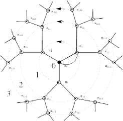
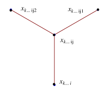
Figure 1. a) Cayley tree of order two with levels 3, b) Elements of the nearest neighborhoods surround the center $x_{k\ldots ij}$, $k=1,2,3$ and $i,j=1,2$.

In the Fig. 1, we show Cayley tree of order two with levels 3 and the nearest neighborhood which comprises three cells which surround the center cell $x_{k\ldots ij}$. The state $x_{k\ldots ij}^{(t+1)}$ of the cell $(i,j)^{\text{th}}$ at time $(t+1)$ is defined by the local rule function $f:\mathbb{F}_{p}^{4}\rightarrow\mathbb{F}_{p}$ as follows:

$$x_{k\ldots ij}^{(t+1)} = f(x_{k\ldots i}^{(t)},x_{k\ldots ij}^{(t)},x_{k\ldots ij1}^{(t)},x_{k\ldots ij2}^{(t)})$$

$$= ax_{k\ldots ij1}^{(t)}+bx_{k\ldots ij2}^{(t)}+cx_{k\ldots i}^{(t)}+dx_{k\ldots ij}^{(t)}(\text{mod }p),$$

where $a,b,c,d\in\mathbb{F}_{p}\setminus\{0\}$, $x_{k\ldots i}^{(t)}\in W_{n-2}$, $x_{k\ldots ij}^{(t)}\in W_{n-1}$ and $x_{k\ldots ij1}^{(t)},x_{k\ldots ij2}^{(t)}\in W_{n}$, $k=1,2,3$ and $i,j=1,2$ (see the Fig. 1 (b)).
Specifically, for state $x_{0}^{(t+1)}$ in the root vertex we can show

(2.2) $$x_{0}^{(t+1)} = f(x_{0}^{(t)},x_{1}^{(t)},x_{2}^{(t)},x_{3}^{(t)})=ax_{1}^{(t)}+bx_{2}^{(t)}+cx_{3}^{(t)}+dx_{0}^{(t)}(\text{mod }p).$$

Function

(2.3) $$T_{f}:\mathbb{F}^{\Gamma^{2}}_{p}\rightarrow\mathbb{F}^{\Gamma^{2}}_{p}$$

is called a cellular automaton (CA) generated by the rules (2) and (2.2). If the boundary cells are connected to 0-state, then CA are called Null Boundary CA, i.e., $V\setminus W_{n}=\{0\}$ for a fixed $n$. If the same rule is applied to all of the cells in ever evaluation, then those CA are called uniform or regular.

In Sections 3 and 4, we consider linear transformations of finite dimensional vectors spaces corresponding to these finite linear cellular automata by imposing the null boundary condition, which means that the states of cells outside a given ball around the origin are fixed to be zero.

3. Construction of the rule matrix in the finite case

In this section, we can characterize finite cellular automata with Null boundary condition over Cayley tree of order two over the field $\mathbb{F}_{p}$. In order to characterize the corresponding rule, first we represent finite Cayley tree $n$ level as a column vector of size $(1+3(2^{n}-1))\times 1.$

Let us denote all configurations of Cayley tree with levels $n$ by $\Omega_{n}$. In order to accomplish this goal we define the following map

$$\Phi:\Omega_{n}\to\mathbb{M}_{(1+3(2^{n}-1))\times 1}(\mathbb{Z}_{p}),$$

which takes the $t^{th}$ state $X^{(t)}$ given by

$$\Omega_{n}\rightarrow X^{(t)}:=\left(x_{0}^{(t)},x_{1}^{(t)},\ldots,x_{21...11}^{(t)},x_{21...12}^{(t)},\ldots,x_{32...211}^{(t)},x_{32...212}^{(t)},x_{32...221}^{(t)},x_{32...222}^{(t)}\right)^{T},$$

where the superscript $T$ denotes the transpose and $\mathbb{M}_{(1+3(2^{n}-1))\times 1}(\mathbb{Z}_{p})$ is the set of matrices with entries $\mathbb{F}_{p}$.

The configuration $\sigma^{(t)}_{n}\in\Omega_{n}$ is called the configuration matrix (or information matrix) of the finite CA on Cayley tree with levels $n$ at time $t$ and $\sigma^{(0)}_{n}$ is initial information matrix of the finite CA. The whole evolution of a particular cellular automata can be comprised in its global transition function [8] (see [8, 23, 24] for the square lattice $\mathbb{F}^{2}$ and see [25] for the hexagonal lattice).

Therefore, one can conclude that $\Phi(\sigma^{(t)}_{n})=X^{(t)}_{(1+3(2^{n}-1))\times 1}$. Using the identification (2.3), due to linearity of the finite CA we can define as follows:

$$(M_{R}^{(n)})_{(1+3(2^{n}-1))\times(1+3(2^{n}-1))}X^{(t)}_{(1+3(2^{n}-1))\times 1}=X^{(t+1)}_{(1+3(2^{n}-1))\times 1},$$

where $n$ is the number of levels of the Cayley tree.

Theorem 3.1.

Let $a,b,c,d\in\mathbb{F}_{p}^{*}=\mathbb{F}_{p}\setminus\{0\},$ $n\geq 2$. Then, the transition rule matrix
$(M_{R}^{(n)})_{1+3(2^{n}-1)\times 1+3(2^{n}-1)}$ corresponding to the finite cellular automata on Cayley tree of order two with $n$-level finite over NB is given by

(3.1) $$\left(\begin{array}[]{cccccccccccccccc}d&P&0_{1\times 6}&\cdots&0&0&0\\ Q&D_{3\times 3}&B_{3\times 6}&0&\cdots&0&0\\ 0&C_{6\times 3}&D_{6\times 6}&B_{6\times 12}&0&\cdots&0\\ \vdots&\vdots&\vdots&\ddots&\ddots&\ddots&\vdots\\ 0&\cdots&0&C_{3.2^{n-3}\times 3.2^{n-4}}&D_{3.2^{n-3}\times 3.2^{n-3}}&B_{3.2^{n-3}\times 3.2^{n-2}}&0\\ 0&0&\cdots&0&C_{3.2^{n-2}\times 3.2^{n-3}}&D_{3.2^{n-2}\times 3.2^{n-2}}&B_{3.2^{n-2}\times 3.2^{n-1}}\\ 0&0&0&\cdots&0&C_{3.2^{n-1}\times 3.2^{n-2}}&D_{3.2^{n-1}\times 3.2^{n-1}}\\ \end{array}\right)$$

where each submatrices are as follows: $P=(\begin{array}[]{ccc}a&b&c\end{array})$, $Q=\left(\begin{array}[]{ccc}c\\ c\\ c\end{array}\right),$

$$C_{3.2^{n-i}\times 3.2^{n-(i+1)}}=\left(\begin{array}[]{cccccccc}c&0&0&0&\cdots&0&0\\ c&0&0&0&\cdots&0&0\\ 0&c&0&0&\cdots&0&0\\ 0&c&0&0&\cdots&0&0\\ \cdots&\cdots&\cdots&\cdots&\cdots&\cdots&\cdots\\ 0&\cdots&\cdots&0&0&c&0\\ 0&0&\cdots&\cdots&0&c&0\\ 0&\cdots&\cdots&0&0&0&c\\ 0&0&\cdots&\cdots&0&0&c\\ \end{array}\right),$$

$$B_{3.2^{n-(i+1)}\times 3.2^{n-i}}=\left(\begin{array}[]{cccccccccc}a&b&0&0&0&0&0&\cdots&0\\ 0&0&a&b&0&0&0&\cdots&0\\ 0&0&0&0&a&b&0&\cdots&0\\ \cdots&\cdots&\cdots&\cdots&\cdots&\cdots&\cdots\\ 0&\cdots&\cdots&0&a&b&0&0&0\\ 0&0&\cdots&\cdots&0&0&0&a&b\\ \end{array}\right),$$

and

$$D_{3.2^{n-i}\times 3.2^{n-i}}=d.I_{3.2^{n-i}\times 3.2^{n-i}}.$$

For $i=1,2,\ldots,n-1.$

In the Theorem 3.1, we have obtained a general form of the matrix representation (or transition rule matrix) for these linear transformations with respect to a basis given by the lexicographical order on the vertices. We do not include a detailed proof of the theorem which gives the rule matrix of CA. The proof is obtained by determining the image of the basis elements of the space $\mathbb{F}_{p}^{(1+3(2^{n}-1))}$ under the CA. These images contribute to the columns of the rule matrix.

Let us illustrate this in Examples 3.1 and 3.2.

Example 3.1.

If we take the number of level as $n=2$, then we get the rule matrix $M_{R}$ of order 10. We consider a configuration $\sigma^{(t)}_{2}$ of number of levels 2 with null boundary:

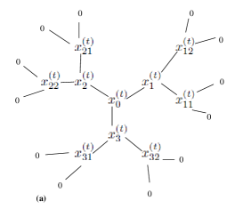
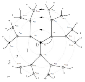
Figure 2. A configuration $\sigma^{(t)}_{2}$ of levels 2 and 3 with null boundary on Cayley tree of order two.

Let us apply the local rules (2) and (2.2) on configuration $\sigma^{(t)}_{2}$ in the Fig 2. Then, we get a new configuration under this transformation which is

$$x_{0}^{(t+1)} = ax_{1}^{(t)}+bx_{2}^{(t)}+cx_{3}^{(t)}+dx_{0}^{(t)};\ x_{1}^{(t+1)}=ax_{11}^{(t)}+bx_{12}^{(t)}+cx_{0}^{(t)}+dx_{1}^{(t)}$$

$$x_{2}^{(t+1)} = ax_{21}^{(t)}+bx_{22}^{(t)}+cx_{0}^{(t)}+dx_{2}^{(t)};\ x_{3}^{(t+1)}=ax_{31}^{(t)}+bx_{32}^{(t)}+cx_{0}^{(t)}+dx_{3}^{(t)}$$

$$x_{11}^{(t+1)} = cx_{1}^{(t)}+dx_{11}^{(t)};\ x_{12}^{(t+1)}=cx_{1}^{(t)}+dx_{12}^{(t)};\ x_{21}^{(t+1)}=cx_{2}^{(t)}+dx_{21}^{(t)}$$

$$x_{22}^{(t+1)} = cx_{2}^{(t)}+dx_{22}^{(t)};\ x_{31}^{(t+1)}=cx_{3}^{(t)}+dx_{31}^{(t)};\ x_{32}^{(t+1)}=cx_{3}^{(t)}+dx_{32}^{(t)}.$$

Hence, we obtain the rule matrix $M_{R}^{(2)}$ of order 10 as follows:

$$M_{R}^{(2)}=\left(\begin{array}[]{c|ccc|cccccc}d&a&b&c&0&0&0&0&0&0\\ \hline\cr c&d&0&0&a&b&0&0&0&0\\ c&0&d&0&0&0&a&b&0&0\\ c&0&0&d&0&0&0&0&a&b\\ \hline\cr 0&c&0&0&d&0&0&0&0&0\\ 0&c&0&0&0&d&0&0&0&0\\ 0&0&c&0&0&0&d&0&0&0\\ 0&0&c&0&0&0&0&d&0&0\\ 0&0&0&c&0&0&0&0&d&0\\ 0&0&0&c&0&0&0&0&0&d\end{array}\right).$$

Example 3.2.

Let us consider the configuration with levels 3 given in the Fig. 2. If we apply the rules (2) and (2.2), then we obtain the following rule matrix $M_{R}^{(3)}$:

$$M_{R}^{(3)} = \left(\begin{array}[]{cccccccccccccccc}d&P&0_{1\times 6}&0\\ Q&D_{3\times 3}&B_{3\times 6}&0\\ 0&C_{6\times 3}&D_{6\times 6}&B_{6\times 12}\\ 0&0&C_{12\times 6}&D_{12\times 12}\\ \end{array}\right)$$

$$= \left(\begin{array}[]{c|ccc|cccccc|cccccccccccc}d&a&b&c&0&0&0&0&0&0&0&0&0&0&0&0&0&0&0&0&0&0\\ \hline\cr c&d&0&0&a&b&0&0&0&0&0&0&0&0&0&0&0&0&0&0&0&0\\ c&0&d&0&0&0&a&b&0&0&0&0&0&0&0&0&0&0&0&0&0&0\\ c&0&0&d&0&0&0&0&a&b&0&0&0&0&0&0&0&0&0&0&0&0\\ \hline\cr 0&c&0&0&d&0&0&0&0&0&a&b&0&0&0&0&0&0&0&0&0&0\\ 0&c&0&0&0&d&0&0&0&0&0&0&a&b&0&0&0&0&0&0&0&0\\ 0&0&c&0&0&0&d&0&0&0&0&0&0&0&a&b&0&0&0&0&0&0\\ 0&0&c&0&0&0&0&d&0&0&0&0&0&0&0&0&a&b&0&0&0&0\\ 0&0&0&c&0&0&0&0&d&0&0&0&0&0&0&0&0&0&a&b&0&0\\ 0&0&0&c&0&0&0&0&0&d&0&0&0&0&0&0&0&0&0&0&a&b\\ \hline\cr 0&0&0&0&c&0&0&0&0&0&d&0&0&0&0&0&0&0&0&0&0&0\\ 0&0&0&0&c&0&0&0&0&0&0&d&0&0&0&0&0&0&0&0&0&0\\ 0&0&0&0&0&c&0&0&0&0&0&0&d&0&0&0&0&0&0&0&0&0\\ 0&0&0&0&0&c&0&0&0&0&0&0&0&d&0&0&0&0&0&0&0&0\\ 0&0&0&0&0&0&c&0&0&0&0&0&0&0&d&0&0&0&0&0&0&0\\ 0&0&0&0&0&0&c&0&0&0&0&0&0&0&0&d&0&0&0&0&0&0\\ 0&0&0&0&0&0&0&c&0&0&0&0&0&0&0&0&d&0&0&0&0&0\\ 0&0&0&0&0&0&0&c&0&0&0&0&0&0&0&0&0&d&0&0&0&0\\ 0&0&0&0&0&0&0&0&c&0&0&0&0&0&0&0&0&0&d&0&0&0\\ 0&0&0&0&0&0&0&0&c&0&0&0&0&0&0&0&0&0&0&d&0&0\\ 0&0&0&0&0&0&0&0&0&c&0&0&0&0&0&0&0&0&0&0&d&0\\ 0&0&0&0&0&0&0&0&0&c&0&0&0&0&0&0&0&0&0&0&0&d\end{array}\right).$$

In order to illustrate the behavior of the finite CA on Cayley tree, we can study the image and preimage under finite CA of a configuration by means of relating matrix and its inverse matrix (see [14]).

4. Reversibility of CA on Cayley tree with Null Boundary

In this section, we characterize finite cellular automata with NBC determined by nearest neighbor rule on Cayley tree. For finite CA, in order to obtain the reversible of a finite CA many authors [5, 6, 7, 11, 12, 13, 24, 25] have used the rule matrices. It is well known that a cellular automaton is reversible if and only if it is bijective [37]. Since we already have found the rule matrix $M_{R}^{(n)}$ corresponding to the the finite CA, by using the matrix in (3.1), we can state the following relation between the column vectors $X^{(t)}$ and the rule matrix $M_{R}$:

$$X^{(t+1)}=M_{R}^{(n)}X^{(t)}\ (\text{mod}\ p).$$

If the rule matrix $M_{R}^{(n)}$ is non-singular, then we have

$$X^{(t)}=(M_{R}^{(n)})^{-1}X^{(t+1)}\ (\text{mod}\ p).$$

Thus, in this paper, one of our main aims is to study whether the rule matrix $M_{R}^{(n)}$ in (3.1) is invertible or not. It is well known that the finite CA is reversible if and only if its rule matrix $M_{R}^{(n)}$ is non-singular (see [5, 6, 7, 24, 25] for details). If the determinant of a matrix is not equal to zero, then it is invertible, so the CA on Cayley tree is reversible, otherwise, it is irreversible. If the CA is not invertible, then one can study ”Garden of Eden” for the finite CA (see [14, 23]).

It is well known that the 1D finite CA is reversible iff its rule matrix $M_{R}^{(n)}$ is non- singular (see [12] for details). An efficient tool to compute the determinant of a matrix $A$ is to multiply all eigenvalues of $A$. So, we conclude that the reversibility of the original system comes from the combination of eigenvalues of these components, so does its inverse [18].

Let us consider matrix $M_{R}^{(n)}$. The characteristic polynomial of the matrix $M_{R}^{(n)}$ is given by

$$\Delta_{M_{R}^{(n)}}(\lambda)=\det(\lambda I-M_{R}^{(n)})=\lambda^{n}+\sum_{i=1}^{n}a_{i}\lambda^{n-i}=\prod_{i=1}^{n}(\lambda-\lambda_{i}).$$

If we assume $\lambda=0$, then from the last equation we have

$$\Delta_{M_{R}^{(n)}}(0)=\det(-M_{R}^{(n)})=(-1)^{n}\det(M_{R}^{(n)})=(-1)^{n}\prod_{i=1}^{n}\lambda_{i}=a_{n}.$$

Therefore, if $\det(M_{R}^{(n)})\neq 0$, then $M_{R}^{(n)}$ is invertible, so corresponding CA is reversible. On the other hand, due to $\det(M_{R}^{(n)})=\prod_{i=1}^{n}\lambda_{i}$, if 0 is not an eigenvalue of $M_{R}^{(n)}$ over $\mathbb{F}_{p}$, then corresponding CA is reversible, where for $(i=1,2,\cdots,3.2^{n}-2)$ $\lambda_{i}$ is an eigenvalue of $M_{R}^{(n)}$.

The following theorem provides basic transitions for reversibility of 1D finite CA on Cayley tree of order 2.

Theorem 4.1.

The linear cellular automaton $T_{f}$ over $\mathbb{F}_{p}$ under null boundary condition is characterized by the matrix $T_{n}$, and vice versa. More explicitly, the diagram

$$\begin{array}[]{ccc}\mathbb{F}^{\Gamma^{2}}_{p}&\overset{T_{f}}{\longrightarrow}&\mathbb{F}^{\Gamma^{2}}_{p}\\ \downarrow\Phi&&\downarrow\Phi\\ \mathbb{Z}_{p}^{1+3(2^{n}-1)}&\underset{\textbf{T}}{\longrightarrow}&\mathbb{Z}_{p}^{1+3(2^{n}-1)}\end{array}$$

commutes, where $\textbf{T}y=T_{f}y\mod p$ for every $y\in\mathbb{F}^{\Gamma^{2}}_{p}.$ Since $\Phi$ is a one-to-one correspondence, the following statements are equivalent

1. $T_{f}$ is reversible;

2. $M_{R}^{(n)}$ is invertible over $\mathbb{F}_{p}$;

3. 0 is not an eigenvalue of $M_{R}^{(n)}$ over $\mathbb{F}_{p}$;

4. The matrix $M_{R}^{(n)}$ has a full rank.

4.1. Illustrative Examples: Reversible

One can compute the determinant of the rule matrix $M_{R}^{(n)}$ for some random $a,b,c,d\in\mathbb{F}_{p}^{*}$ and the levels $n$ of Cayley tree as follows:

$$\det(M_{R}^{(2)})=d^{4}(d^{2}-c(2(a+b)+c))(d^{2}-(a+b)c)^{2}$$

$$\det(M_{R}^{(3)})=d^{8}(d^{2}-(a+b)c)^{3}(d^{2}-2(a+b)c)^{2}((a+b)c^{2}(a+b+c)-c(3(a+b)+c)d^{2}+d^{4}).$$

We have seen that the CAs are reversible for some given values $a,b,c,d\in\mathbb{F}_{p}^{*}$ and $n$, for some values the CAs are irreversible.

Notably, the eigenvalues of the matrix $M_{R}^{(2)}$ are $d,d,d,d,d-\sqrt{ac+bc},d-\sqrt{ac+bc},\sqrt{ac+bc}+d,\sqrt{ac+bc}+d,d-\sqrt{2ac+2bc+c^{2}},\sqrt{2ac+2bc+c^{2}}+d$, respectively. The last situation reveals that the necessary and sufficient conditions for the matrix $M_{R}^{(2)}$ being invertible are

$$\left\{\begin{array}[]{l}\sqrt{ac+bc}\neq d(\text{mod}p);\\ \sqrt{2ac+2bc+c^{2}}\neq d(\text{mod}p).\end{array}\right.$$

Therefore, the CA corresponding to the matrix $M_{R}^{(2)}$ is reversible if and only if

$$\left\{\begin{array}[]{l}\sqrt{ac+bc}\neq d(\text{mod}p);\\ \sqrt{2ac+2bc+c^{2}}\neq d(\text{mod}p).\end{array}\right.$$

In the Table 1, we examine under what conditions these linear transformations are invertible, and check invertibility for a list of parameters using computations by means of ”Mathematica”. For example, if we take as $a=b=c=d=1$ and $n=3$, then we can see that the CAs are irreversible for prime numbers $p<47$. The reversibility of finite CAs on Cayley tree of order two is determined for some given values of $a,b,c,d\in\mathbb{F}_{p}^{*}$ and the levels $n$ of Cayley tree. One can fully characterize reversibility of finite cellular automata with NBC determined by nearest neighbor rule on Cayley tree by computing the determinant of the matrix in the Eq. (3.1). Also, one can study the reversibility of finite CAs via rank of the matrix in the Eq. (3.1) (see [25]).

Table 1. The reversibility of finite CAs for some given $a,b,c,d\in\mathbb{F}_{p}^{*}$ and the levels $n=2,3$ of Cayley tree of order two.

$a$	$b$	$c$	$d$	$n$	$p$	reversibility of finite CA
1	1	1	1	2	2	irreversible
1	1	1	1	2	3,5,…,101	reversible
2	1	5	2	2	17	irreversible
2	1	3	2	2	17	reversible
2	3	4	3	2	11	irreversible
1	1	1	1	3	3	irreversible
2	2	3	3	3	5	irreversible
2	1	1	3	3	5	reversible
2	2	3	3	3	7,11,13,19,23,29	reversible

5. The measure entropy of the CA on Cayley tree

In this section we study the measure entropy of cellular automata defined by local rules in (2) and (2.2) on Cayley tree of order two. In order to state our result, we first recall necessary definitions. Let $(X,\mathcal{B},\mu,T)$ be a measure-theoretical dynamical system. If $\alpha=\{A_{1},\ldots,A_{n}\}$ and $\beta=\{B_{1},\ldots,B_{m}\}$ are two measurable partitions of $X$, then $\alpha\vee\beta=\{A_{i}\cap B_{j}:i=1,\ldots,n;j=1,\ldots,m\}$ is the partition of $X$. Also, $T^{-1}\alpha$ is the partition of $X$ and $T^{-1}\alpha=\{T^{-1}A_{1},\ldots,T^{-1}A_{n}\}$ (see [26, 27] for details).

Definition 5.1.

Let $\alpha$ be a measurable partition of $X$. The quantity

$$H_{\mu}(\alpha)=-{\underset{A\in\alpha}{\sum}}\mu(A)\log\mu(A)$$

is called the entropy of the partition $\alpha$. The logarithm is usually taken to the base 2. Let $\alpha$ be a partition with finite entropy, then the quantity

$$h_{\mu}(T,\alpha)=\overset{}{\underset{n\rightarrow\infty}{\lim}}\frac{1}{n}H_{\mu}(\overset{n-1}{\underset{i=0}{\bigvee}}T^{-i}\alpha)$$

is called the entropy of $\alpha$ with respect to $T$. The quantity

(5.1) $$h_{\mu}(T)=\overset{}{\underset{\alpha}{\sup}}\{h_{\mu}(T,\alpha):\alpha\ \text{is a partition with}\ H_{\mu}(\alpha)<\infty\}$$

is called the measure-theoretical entropy of $(X,\mathcal{B},\mu,T)$, the entropy of $T$ (with respect to $\mu$).

Let $\pi=\{\pi_{0},\pi_{1},\ldots,\pi_{p-1}\}$ be a probability vector. Recall that the Bernoulli measure is defined as follows:

$$\mu_{\pi}(_{0}[i_{0},\ldots,i_{k}]_{k})=\pi_{i_{1}}\pi_{i_{0}}\ldots\pi_{i_{k}},$$

where ${}_{0}[i_{0},\ldots,i_{k}]_{k}$ is a cylinder set (see [26, 27] for details). If we take the Bernoulli measure as

$$\mu_{\pi}(_{0}[i_{0},\ldots,i_{k}]_{k})=\frac{1}{p}\frac{1}{p}\cdots\frac{1}{p}=\frac{1}{p^{k+1}},$$

then the measure is called uniform Bernoulli measure, i.e., for all $i\in\mathbb{F}_{p}$, $\mu_{\pi}(_{0}[i])=\frac{1}{p}$, then $\mu_{\pi}$ is the uniform Bernoulli measure on the space $\mathbb{F}^{\Gamma^{2}}_{p}$. In this paper, we consider uniform Bernoulli measure.

It is clear that due to $(a,p)=1,(b,p)=1,(c,p)=1$ and $(d,p)=1$, the rules given in the Eqs. (2) and (2.2) are bipermutative. The following Theorems have been proved:

Theorem 5.2.

[28] Any left-permutative (right-permutative) cellular is surjective (see [29] for details).

Theorem 5.3.

[30] If a cellular automaton is surjective then it preserves a uniform Bernoulli measure.

D’amico et al. [17] have proved that for $D$-dimensional linear CA with $D\geq 2$ the topological entropy must be 0 or infinity (see [31]). In the one-dimensional case, the measure theoretical entropy of the cellular automata is finite [1, 30]. In the following theorem, we prove that the linear CA on Cayley tree of order two has infinite entropy.

Let us choose $a,b,c,d\in\mathbb{F}_{p}^{*}$ such that the cellular automata $T_{f}$ defined in the Eq. (2.3) is measure-preserving function with respect to (w.r.t.) the uniform Bernoulli measure on the space $\mathbb{F}^{\Gamma^{2}}_{p}$. Then we have the following theorem.

Theorem 5.4.

Let $T_{f}$ be cellular automata defined by local rules in (2) and (2.2) on Cayley tree of order two over the field $\mathbb{F}_{p}$. Then the measure theoretical entropy of $T_{f}$ w.r.t. the uniform Bernoulli measure on the space $\mathbb{F}^{\Gamma^{2}}_{p}$ is infinity.

Proof.

From theorems 5.2 and 5.3, we note that $\mu_{\pi}$ is a $T_{f}$-invariant measure. Let the zero-time partition be given as $\xi(0,1)=\{_{0}[0],_{0}[1],\ldots,_{0}[p-1]\},$ we put $\xi(-i,i)=\bigvee_{u=-i}^{i}\sigma^{-u}\xi$, where $\sigma$ is the shift map. Since $T_{f}$ is permutative, one has

$$\bigvee_{k=0}^{n-1}T_{f}^{-k}\xi(0,1) = \xi(0,1+3(2^{n}-1)).$$

From the definition of measure theoretical entropy w.r.t the measure, we get

$$h_{\mu_{\pi}}(T_{f},\xi(0,1)) = {\underset{n\rightarrow\infty}{\lim}}\frac{1}{n}H_{\mu_{\pi}}(\overset{n-1}{\underset{k=0}{\bigvee}}T_{f}^{-k}\xi(0,1))$$

$$= -{\underset{n\rightarrow\infty}{\lim}}\frac{1}{n}{\underset{A\in\xi(0,1+3(2^{n}-1))}{\sum}}\mu_{\pi}(A)\log\mu_{\pi}(A)$$

$$= -{\underset{n\rightarrow\infty}{\lim}}\frac{1}{n}p^{1+3(2^{n}-1)}\frac{1}{p^{1+3(2^{n}-1)}}\log\frac{1}{p^{1+3(2^{n}-1)}}$$

$$= {\underset{n\rightarrow\infty}{\lim}}\frac{1}{n}(1+3(2^{n}-1))\log p=\infty.$$

Therefore, from the Eq. (5.1), one can conclude that $h_{\mu_{\pi}}(T_{f})=\infty.$ ∎

Remark 5.1.

If we choose the probability vector as $\pi=(1,0,\ldots,0)$, then
$h_{\mu_{\pi}}(T_{f},\xi(0,1))=0$.

6. Conclusions

In this short paper, firstly we have defined linear cellular automata on Cayley tree of order 2. We have constructed the rule matrix corresponding to finite cellular automata on Cayley tree by using matrix algebra built on the field $\mathbb{F}_{p}$ (the set of prime numbers modulo $p$). Further, we have discussed the reversibility problem of this cellular automata. Lastly, we have studied the measure theoretical entropy of the cellular automata on Cayley tree.

To the best knowledge of the author, it is believed that this is the first instance in the literature where such a connection is established. Thus, this connection between cellular automata and Cayley tree leads to many questions and applications that wait to be explored.

Using the methods in the references [32, 34, 35, 36], we will demonstrate the application of linear rules on image matrix which forms the basis of self replicating and self-similar patterns in image processing on Cayley tree. Also, investigation of CA on Cayley tree with more higher orders will be studied in the future works.

References

• [1] H. Akın, On the measure entropy of additive CA $f_{\infty}$, Entropy 5 (2003) 233-238.
• [2] H. Akın, The measure-theoretic entropy of linear cellular automata with respect to a Markov measure, Bulletin of the Malaysian Mathematical Sciences Society, 35(1) (2012), 171 178.
• [3] H. Akın, I. Siap, S. Uguz, One-dimensional cellular automata with reflective boundary conditions and radius three, Acta Physica Polonica A, 125 (2), (2014) 405-407.
• [4] P. Chattopadhyay, P. P. Choudhury and K. Dihidar, Characterization of a particular hybrid transformation of two-dimensional cellular automata, Comput. Math. Appl. 38 (1999) 207-216.
• [5] A. R. Khan, P. P. Choudhury, K. Dihidar, S. Mitra, P. Sarkar, VLSI architecture of a cellular automata machine, Comput. Math. Appl. 33 (1997) 79-94.
• [6] A. R. Khan, P. P. Choudhury, K. Dihidar, R. Verma, Text compression using two dimensional cellular automata, Comput. Math. Appl. 37 (1999) 115-127.
• [7] Z. Ying, Y. Zhong and D. Pei-min, On behavior of two-dimensional cellular automata with an exceptional rule, Inform. Sci. 179 (2009) 613-622.
• [8] K. Dihidar, P.P. Choudhury, Matrix Algebraic formulae concerning some special rules of two-dimensional Cellular Automata, Inform. Sci. 165 (2004) 91-101.
• [9] J. von Neumann, Collected Works, Design of Computers Theory of Automata and Numerical Analysis, Vol. 5, (Pergamon Press, 1951).
• [10] N.Y. Soma, J.P. Melo, On irreversibility of von Neumann additive cellular automata on grids, Disc. Appl. Math. 154 (2006) 861-866.
• [11] H. Akın, F. Sah, I. Siap, On 1D reversible cellular automata with reflective boundary over the prime field of order $p$, Internat. J. Modern Phys. C, 23 (2012) 1-13.
• [12] Z. Cinkir, H. Akın, I. Siap, Reversibility of 1D cellular automata with periodic boundary over finite fields $Z_{p},$ J. Stat. Phys. 143 (2011) 807-823.
• [13] A. Martín del Rey, A note on the reversibility of elementary cellular automaton 150 with periodic boundary conditions, Romanian Journal of Information Science and Technology, 16 (4) (2013), 365 372
• [14] G. Fici and F. Fiorenzi, Topological properties of cellular automata on trees, AUTOMATA 2012, Elec. Proc. in Theoret. Comput. Sci. 90 (2012) 255-266.
• [15] H. Akın, The topological entropy of $n$th iteration of an additive cellular automata, Appl. Math. Comput. 174 (2006) 1427-1437.
• [16] H. Akın, Upper bound of the directional entropy of a $Z^{2}$-action, Internat. J. Modern Phys. C 22 (2011) 711-718.
• [17] M. D’amico, G. Manzini and L. Margara, On computing the entropy of cellular automata, Theor. Comput. Sci. 290 (2003) 1629-1646.
• [18] Chang, C. H., Su, J.Y., Akın, H., & Sah, F., Reversibility problem of multidimensional finite cellular automata, J. Stat. Phys., 168 (1), 208-231 (2017) DOI: 10.1007/s10955-017-1799-6
• [19] G. Morris, T. Ward, Entropy bounds for endomorphisms commuting with $K$ actions, Israel J. Math. 106 (1998) 1-12.
• [20] T. Meyerovitch, Finite entropy for multidimensional cellular automata, Ergodic Theory and Dynam. Systems 28 (2008)1243-1260.
• [21] F. Blanchard and P. Tisseur, Entropy rate of higher-dimensional cellular automata, arXiv:1206.6765.
• [22] L. Accardi, F. Mukhamedov and M. Saburov, On quantum Markov chains on Cayley tree I: Uniqueness of the associated chain with $XY$-model on the Cayley tree of order two, Infin. Dimens. Anal. Quantum Probab. Relat. 14 (2011) 443-463.
• [23] I. Siap, H. Akın and F. Sah, Garden of eden configurations for 2-D cellular automaton with rule 2460N, Inform. Sci. 180 (2010) 3562-3571.
• [24] I. Siap, H. Akin and F. Sah, Characterization of two dimensional cellular automata over ternary fields, J. Franklin Inst. 348 (2011) 1258-1275.
• [25] I. Siap, H. Akın, and S. Uguz, Structure and reversibility of 2-dimensional hexagonal cellular automata, Comput. Math. Appl. 62 (2011) 4161-4169.
• [26] M. Denker, C. Grillenberger and K. Sigmund, Ergodic theory on compact spaces. Springer Lectures Notes in Math. 527 Springer Verlag, 1976.
• [27] P. Walters, An Introduction to Ergodic Theory, Springer Graduate Texts in Math. 79 New York, 1982.
• [28] G. A. Hedlund, Endomorphisms and automorphisms of full shift dynamical system, Math. Syst. Theory 3 (1969) 320-375.
• [29] M. A. Shereshevsky, Ergodic properties of certain surjective cellular automata, Mh. Math. 114 (1992) 305-316.
• [30] F. Blanchard, P. Kurka and A. Maass, Topological and Measure-Theoretic Properties of One-Dimensional Cellular Automata, Physica D 103 (1997) 86 89.
• [31] G. Manzini, L. Margara, A complete and efficiently computable topological classification of linear cellular automata over $\mathbb{Z}_{m}$, Theoret. Comput. Sci. 221 (1999) 157-177.
• [32] U. Sahin, S. Uguz, H. Akın, and I. Siap, Three-state von Neumann cellular automata and pattern generation, Applied Mathematical Modelling 39, no. 7 (2015) 2003-2024.
• [33] M. Koroglu, I. Siap, and H. Akın, Error correcting codes via reversible cellular automata over finite fields, Arab. J. Sci. Eng. 39, no. 3 (2014): 1881-1887.
• [34] S. Uguz, U. Sahin, H. Akın, and I. Siap, Self-replicating patterns in 2D linear cellular automata, Int. J Bifurcat. Chaos, 24, no. 01 (2014) 1430002.
• [35] S. Uguz, U. Sahin, H. Akın, and I. Siap, 2D cellular automata with an image processing application, Acta Phys. Polon. A 125, (2014) 435 438.
• [36] U. Sahin, S. Uguz, H. Akın, The transition rules of 2D linear cellular automata over ternary field and self-replicating patterns, Int. J Bifurcat. Chaos, 25 (01), (2015) 1550011.
• [37] J. Kari, Reversibility of 2D cellular automata is undecidable, Phys. D 45, no. 1-3, 379-385 (1990).
• [38] H. Akın, The topological entropy of invertible cellular automata, J. Computation and Appl. Math. 213, 501-508 (2008).
• [39] H. Akın, S. Uguz, I. Siap, Characterization of 2D cellular automata with Moore neighborhood over ternary fields, AIP Conf. Proc. 1389, (2011), 2008-2011.
• [40] Koroglu, M. E., Siap, I., & Akın, H., The reversibility problem for a family of two-dimensional cellular automata, Turkish Journal of Mathematics, 40, 665-678 (2016), DOI: 10.3906/mat-1503-18