Correlation functions in one-dimensional spin lattices with Ising and Heisenberg bonds

Stefano Bellucci INFN-Laboratori Nazionali di Frascati, Via E. Fermi 40, 00044 Frascati, Italy    Vadim Ohanyan Department of Theoretical Physics, Yerevan State University, Alex Manoogian 1, 0025 Yerevan, Armenia ICTP, Strada Costiera 11, I-34151 Trieste, Italy
Abstract

A general technique of exact calculation of any correlation functions for the special class of one-dimensional spin models containing small clusters of quantum spins assembled to a chain by alternating with the single Ising spins is proposed. The technique is a natural generalization of that in the models solved by a classical transfer matrix. The general expressions for corresponding matrix operators which are the key components of the technique are obtained. As it is clear from the general principles, the decay of the correlation functions of various types is explicitly shown to be governed by a single correlation length. The technique is illustrated by two examples: symmetric diamond chain and asymmetric sawtooth chain.

Heisenberg-Ising chains, correlation functions, classical transfer matrix, diamond chain, sawtooth chain
pacs:
75.10.Jm

I Introduction

Recently, much attention has been paid to the exactly solvable models of one-dimensional magnetism, consisting of small quantum spin clusters connected to each other via Ising spins.str03 ; str04 ; str05 ; can06 ; val08 ; per08 ; per09 ; str09 ; ant09 ; oha09 ; oha10 ; str10 ; bel10 ; roj11a ; roj11b ; lis11a ; lis11b ; str11 ; oha12 ; cha12 ; roj12a ; ana12 ; ver12 ; str12 ; gal ; roj12b For the sake of simplicity we will call them Heisenberg–Ising chains (HIC). The interest toward such spin systems stems from several features they possess. First of all, they allow one to obtain an exact statistical-mechanical solution of the problem of strongly interacting spins in terms of classical transfer matrixbax ; oha03 ; ayd05 ; ayd06 . In addition to that, such systems combine the quantum and classical properties and also, to some extent, are connected to the problems and models of molecular magnetismmol_mag , as the classical transfer matrix is constructed by the diagonalization of the small quantum spin cluster. And finally, very recently the family of trimetallic coordination polymer compounds has been synthesizedchem ; ring ; Dy_10 . These compounds in the magnetic sense are indeed a one-dimensional magnets with both classical (Ising) and quantum (Heisenberg) bonds. The single-chain magnet reported in Ref. chem, is an example of a Heisenberg-Ising chain of triangles with three-spin linear quantum clusters; another interesting molecular magnet (spin ring) based on the highly anisotropic properties of the Dy3+ ions has been reported in Ref. ring, . Both systems have been analyzed by the transfer-matrix solution of HIC chains in Ref. Dy_10, . Another class of examples is given by chain magnets with two alternating magnetic ions, thus giving rise to alternating quantum and classical spins (see, e.g., Refs. RCRS04, ; JACS10, ; SSR11, ). Let us describe the general scheme of the HIC:

  • There is a small cluster of a few quantum spins with a certain topology of bonds which could contain various types of spin-spin interaction as well as interactions with external fields. The Hamiltonian of the single small cluster is, thus, a finite dimensional matrix.

  • These clusters are assembled to the chain or any other one-dimensional structure by alternating with the single Ising spins.

  • The interaction between the single Ising spins and any quantum spin from a small cluster must contain only z𝑧z-components (Ising interaction).

For the mixed quantum–classical spin system with the above mentioned properties the exact solution is obtained in the following way. The idea is to apply a classical transfer-matrix formalism in which the entries of the classical transfer matrix are obtained from the diagonalization of a small quantum spin cluster. Although the number of papers devoted to the exact solutions of the HIC and to their magneto-thermal properties is rather impressive, only a few models have been solved within the classical transfer matrix formalismval08 ; ant09 ; oha09 ; oha10 ; bel10 ; roj11a ; roj11b ; lis11a ; lis11b ; oha12 ; cha12 ; roj12a ; ana12 ; roj12b , while the other method of the so-called decoration iteration transformation has been also usedstr03 ; str04 ; str05 ; can06 ; str09 ; str10 ; str12 ; gal . Particularly, within the direct classical transfer matrix technique the following models have been solved exactly: the double-tetrahedral chain with quantum triangles of spinsant09 ; oha10 , the sawtooth chain with an asymmetric pair of quantum spinsoha09 ; bel10 , diamond chainroj11a ; lis11a ; lis11b ; cha12 ; roj12a ; ana12 ; roj12b and orthogonal-dimer chain with anisotropic and asymmetric quantum trianglesoha12 . Despite the complete and exact description of the ground states and ground states phase diagrams, as well of all thermodynamic functions, finite-temperature entropy and magnetization, magnetocaloric effect, etc, the expressions for the correlation function are still missing. It is worth mentioning, that the correlation functions can be in principle calculated by another method which is used to handle the HIC, the technique of the decoration iteration transformationstr03 ; str04 ; str05 ; can06 ; str09 ; str10 ; str12 ; gal ; fisher ; roj09 ; str10c . However, the method of the classical transfer matrix is more straightforward and is based on a direct application of the canonical expectation valueskne ; lyra , which can be calculated exactly. In the present paper we are going to develop an exact technique for the calculation of any finite-temperature correlation function for any HIC by means of the direct application of the classical transfer-matrix method.

Beside the pure academic interest, the knowledge about the exact correlation functions of the HIC recently became important from the experimental point of view as well. As mentioned above, a few years ago it was reported about the synthesis of a novel class of trimetallic coordination polymer compoundschem ; ring ; Dy_10 ; JACS10 ; SSR11 which are the real examples of the HIC (at least one of them). As known, the neutron scattering is one of the most powerful and straightforward methods of investigation of the magnetic structure, spin textures, magnetic excitations, etc. In the leading order the cross-section of the neutron scattering is given by the two-point spin-spin correlation functions (their Fourier-transform). This fact makes the topic of the present paper a practical issue.

The paper is organized as follows. In the second Section we remind the reader of the main features of the classical transfer-matrix formalism for the HIC, in the next section we present the formalism for calculating the correlation function of HIC in terms of traces of certain matrix products and prove that for all kinds of correlation functions the correlation length is the same. In Section IV we apply the general formalism for several models. The paper ends with a Conclusion.

II Classical transfer-matrix formalism for HIC

The Hamiltonian of a HIC has the form of a sum of local block Hamiltonians nsubscript𝑛{\mathcal{H}}_{n} which correspond to the n-th small quantum cluster and its interaction with left and right Ising spins:

=n=1N(nH2(σn+σn+1)),superscriptsubscript𝑛1𝑁subscript𝑛𝐻2subscript𝜎𝑛subscript𝜎𝑛1{\mathcal{H}}=\sum_{n=1}^{N}\left({\mathcal{H}}_{n}-\frac{H}{2}\left(\sigma_{n}+\sigma_{n+1}\right)\right), (1)

here σnsubscript𝜎𝑛\sigma_{n} is the Ising spin situated between the n-th and (n+1)-th small cluster and H𝐻H is the magnetic field acting on Ising spins. The block Hamiltonian can contain various terms with quantum and classical spin variables which are determined by the topology of the elementary block and the character of interactions. Let us denote the quantum spins by 𝐒𝐒\mathbf{S}; then one can suppose that the block Hamiltonian depends on 𝐒𝐒\mathbf{S}, σ𝜎\sigma and may be on other classical spins τbsubscript𝜏𝑏\tau_{b},

n=(𝐒n,a,σn,σn+1,τn,b).subscript𝑛subscript𝐒𝑛𝑎subscript𝜎𝑛subscript𝜎𝑛1subscript𝜏𝑛𝑏\displaystyle{\mathcal{H}}_{n}={\mathcal{H}}\left({\mathbf{S}}_{n,a},\sigma_{n},\sigma_{n+1},\tau_{n,b}\right). (2)

Due to the properties listed above the block Hamiltonians commute to each other,

[i,j]=0.subscript𝑖subscript𝑗0\left[{\mathcal{H}}_{i},{\mathcal{H}}_{j}\right]=0. (3)

This fact allows one to expand the exponential in the expression for the partition function of the model and obtain an expression which by its structure corresponds to the classical transfer matrix scheme:

𝒵𝒵\displaystyle{\mathcal{Z}} =\displaystyle= TrS(σ)(τ)exp(β)=(σ)n=1NeβH2(σn+σn+1)(τ)Trneβn=subscriptTrSsubscript𝜎subscript𝜏𝛽subscript𝜎superscriptsubscriptproduct𝑛1𝑁superscript𝑒𝛽𝐻2subscript𝜎𝑛subscript𝜎𝑛1subscript𝜏subscriptTr𝑛superscript𝑒𝛽subscript𝑛absent\displaystyle{\mathrm{Tr}}_{{\mathrm{S}}}\sum_{(\sigma)}\sum_{(\tau)}\exp\left(-\beta{\mathcal{H}}\right)=\sum_{(\sigma)}\prod_{n=1}^{N}e^{\beta\frac{H}{2}\left(\sigma_{n}+\sigma_{n+1}\right)}\sum_{(\tau)}{\mathrm{Tr}}_{n}e^{-\beta{\mathcal{H}}_{n}}=
(σ)n=1NeβH2(σn+σn+1)(τ)i=1Leβλi(σn,σn+1|τn,b)=(σ)n=1NTσn,σn+1=Tr𝐓N,subscript𝜎superscriptsubscriptproduct𝑛1𝑁superscript𝑒𝛽𝐻2subscript𝜎𝑛subscript𝜎𝑛1subscript𝜏superscriptsubscript𝑖1𝐿superscript𝑒𝛽subscript𝜆𝑖subscript𝜎𝑛conditionalsubscript𝜎𝑛1subscript𝜏𝑛𝑏subscript𝜎superscriptsubscriptproduct𝑛1𝑁subscript𝑇subscript𝜎𝑛subscript𝜎𝑛1Trsuperscript𝐓𝑁\displaystyle\sum_{(\sigma)}\prod_{n=1}^{N}e^{\beta\frac{H}{2}\left(\sigma_{n}+\sigma_{n+1}\right)}\sum_{(\tau)}\sum_{i=1}^{L}e^{-\beta\lambda_{i}\left(\sigma_{n},\sigma_{n+1}|\tau_{n,b}\right)}=\sum_{(\sigma)}\prod_{n=1}^{N}T_{\sigma_{n},\sigma_{n+1}}={\mathrm{Tr}}\mathbf{T}^{N},

here the cyclic boundary conditions are supposed, λi(σn,σn+1|τn,b)subscript𝜆𝑖subscript𝜎𝑛conditionalsubscript𝜎𝑛1subscript𝜏𝑛𝑏\lambda_{i}(\sigma_{n},\sigma_{n+1}|\tau_{n,b}) are the eigenvalues of the block Hamiltonian nsubscript𝑛{\mathcal{H}}_{n}(which is supposed to be an L𝐿L by L𝐿L matrix ) depending on the values of classical spins τ𝜏\tau and classical spins σnsubscript𝜎𝑛\sigma_{n} which alternate with the blocks, TrnsubscriptTr𝑛{\mathrm{Tr}}_{n} means the trace over the states of the n𝑛n-th quantum block, and TrTr{\mathrm{Tr}} stands for the trace of the 2 by 2 transfer matrix with entries Tσn,σn+1subscript𝑇subscript𝜎𝑛subscript𝜎𝑛1T_{\sigma_{n},\sigma_{n+1}}. After summation over the values of τ𝜏\tau for each block one gets the expression depending only on σnsubscript𝜎𝑛\sigma_{n} and σn+1subscript𝜎𝑛1\sigma_{n+1} which is the classical 2 by 2 transfer matrix

𝐓=(eβH2Z++Z+Z+eβH2Z),𝐓superscript𝑒𝛽𝐻2subscript𝑍absentsubscript𝑍absentmissing-subexpressionsubscript𝑍absentsuperscript𝑒𝛽𝐻2subscript𝑍absentmissing-subexpression\displaystyle\mathbf{T}=\left(\begin{array}[]{lcr}e^{\beta\frac{H}{2}}Z_{++}&Z_{+-}\\ Z_{-+}&e^{-\beta\frac{H}{2}}Z_{--}\end{array}\right), (7)

where Zσn,σn+1=(τ)i=1Leβλi(σn,σn+1|τn,b)subscript𝑍subscript𝜎𝑛subscript𝜎𝑛1subscript𝜏superscriptsubscript𝑖1𝐿superscript𝑒𝛽subscript𝜆𝑖subscript𝜎𝑛conditionalsubscript𝜎𝑛1subscript𝜏𝑛𝑏Z_{\sigma_{n},\sigma_{n+1}}=\sum_{(\tau)}\sum_{i=1}^{L}e^{-\beta\lambda_{i}\left(\sigma_{n},\sigma_{n+1}|\tau_{n,b}\right)} is the partition function of one block, depending on the values of two neighboring Ising spins, signs ”++” and ”-” in indexes correspond to σ=1/2𝜎12\sigma=1/2 and σ=1/2𝜎12\sigma=-1/2 respectively. The formalism of classical transfer-matrix allows one to obtain exact analytic expressions for almost any expectation values of the function of local variables (spins) and, of course, for any thermodynamic functions, as the expression for the free energy per block can be obtained in a straightforward way by finding the maximal eigenvalue of the transfer matrix (7):

f=1βlog12(eβH2Z+++eβH2Z+(eβH2Z++eβH2Z)2+4Z+Z+).𝑓1𝛽12superscript𝑒𝛽𝐻2subscript𝑍absentsuperscript𝑒𝛽𝐻2subscript𝑍absentsuperscriptsuperscript𝑒𝛽𝐻2subscript𝑍absentsuperscript𝑒𝛽𝐻2subscript𝑍absent24subscript𝑍absentsubscript𝑍absent\displaystyle f=-\frac{1}{\beta}\log\frac{1}{2}\left(e^{\beta\frac{H}{2}}Z_{++}+e^{-\beta\frac{H}{2}}Z_{--}+\sqrt{\left(e^{\beta\frac{H}{2}}Z_{++}-e^{-\beta\frac{H}{2}}Z_{--}\right)^{2}+4Z_{+-}Z_{-+}}\right). (8)

From this expression any thermodynamic function, like magnetization, entropy, specific head etc can be obtained exactly. However, to obtain correlation functions of the spins demands more efforts and further development of the classical transfer-matrix technique.

III Correlation functions and correlation length

Let us concentrate on the scheme of calculation of the expectation values of combinations of spins operators. First of all, let us start from the simplest case, the expectation values of σ𝜎\sigma-s, which is quite similar to that of the Ising chainbax . Thus, for the thermodynamic average of just one σ𝜎\sigma one obtains

σjdelimited-⟨⟩subscript𝜎𝑗\displaystyle\langle\sigma_{j}\rangle =1𝒵(σ)σjn=1NTσn,σn+1absent1𝒵subscript𝜎subscript𝜎𝑗superscriptsubscriptproduct𝑛1𝑁subscript𝑇subscript𝜎𝑛subscript𝜎𝑛1\displaystyle=\frac{1}{{\mathcal{Z}}}\sum_{(\sigma)}\sigma_{j}\prod_{n=1}^{N}T_{\sigma_{n},\sigma_{n+1}} (9)
=1𝒵(σ)Tσ1,σ2σjTσj,σj+1TσN,σ1.absent1𝒵subscript𝜎subscript𝑇subscript𝜎1subscript𝜎2subscript𝜎𝑗subscript𝑇subscript𝜎𝑗subscript𝜎𝑗1subscript𝑇subscript𝜎𝑁subscript𝜎1\displaystyle=\frac{1}{{\mathcal{Z}}}\sum_{(\sigma)}T_{\sigma_{1},\sigma_{2}}...\sigma_{j}T_{\sigma_{j},\sigma_{j+1}}...T_{\sigma_{N},\sigma_{1}}.

This expression is the trace of the product of N𝑁N transfer-matrices with the matrix

σz=(1/2001/2)superscript𝜎𝑧120missing-subexpression012missing-subexpression\displaystyle{\mathbf{\sigma}}^{z}=\left(\begin{array}[]{lcr}1/2&0\\ 0&-1/2\end{array}\right) (12)

inserted before the j𝑗j-th transfer matrix in the trace formula. Thus, we have

σj=1𝒵𝐓𝐫(σz𝐓N)=1𝒵𝐓𝐫(σz𝐀𝚲N𝐀1),delimited-⟨⟩subscript𝜎𝑗1𝒵𝐓𝐫superscript𝜎𝑧superscript𝐓𝑁1𝒵𝐓𝐫superscript𝜎𝑧𝐀superscript𝚲𝑁superscript𝐀1\displaystyle\langle\sigma_{j}\rangle=\frac{1}{{\mathcal{Z}}}{\mathbf{Tr}}\left({\mathbf{\sigma}}^{z}{\mathbf{T}}^{N}\right)=\frac{1}{{\mathcal{Z}}}{\mathbf{Tr}}\left({\mathbf{\sigma}}^{z}{\mathbf{A}}{\mathbf{\Lambda}}^{N}{\mathbf{A}}^{-1}\right), (13)

where we used the matrix identity 𝐓=𝐀𝚲𝐀1𝐓𝐀𝚲superscript𝐀1{\mathbf{T}}={\mathbf{A}}{\mathbf{\Lambda}}{\mathbf{A}}^{-1}, with the diagonal matrix 𝚲𝚲{\mathbf{\Lambda}} and the orthogonal matrix 𝐀𝐀{\mathbf{A}}. Thus,

𝚲=(λ100λ2),𝐀=(cosϕsinϕsinϕcosϕ),formulae-sequence𝚲subscript𝜆10missing-subexpression0subscript𝜆2missing-subexpression𝐀italic-ϕitalic-ϕmissing-subexpressionitalic-ϕitalic-ϕmissing-subexpression\displaystyle{\mathbf{\Lambda}}=\left(\begin{array}[]{lcr}\lambda_{1}&0\\ 0&\lambda_{2}\end{array}\right),\qquad{\mathbf{A}}=\left(\begin{array}[]{lcr}\cos\phi&-\sin\phi\\ \sin\phi&\cos\phi\end{array}\right), (18)

where λ1,2subscript𝜆12\lambda_{1,2} are the eigenvalues of the transfer-matrix, and ϕitalic-ϕ\phi is a parameter. Having all these notations we now can express the canonical expectation values from Eq. (9) in terms of the entries of the orthogonal matrix diagonalizing the transfer-matrix. Using the properties of the trace (cyclic permutation inside the trace does not change it) one can get

σjdelimited-⟨⟩subscript𝜎𝑗\displaystyle\langle\sigma_{j}\rangle =\displaystyle= 1𝒵𝐓𝐫(𝐀1σz𝐀𝚲N)=1𝒵𝐓𝐫superscript𝐀1superscript𝜎𝑧𝐀superscript𝚲𝑁absent\displaystyle\frac{1}{{\mathcal{Z}}}{\mathbf{Tr}}\left({\mathbf{A}}^{-1}{\mathbf{\sigma}}^{z}{\mathbf{A}}{\mathbf{\Lambda}}^{N}\right)= (19)
12(cos2ϕ)λ12(sin2ϕ)λ2Nλ1N+λ2N122italic-ϕsuperscriptsubscript𝜆122italic-ϕsuperscriptsubscript𝜆2𝑁superscriptsubscript𝜆1𝑁superscriptsubscript𝜆2𝑁\displaystyle\frac{1}{2}\frac{(\cos 2\phi)\lambda_{1}^{2}-(\sin 2\phi)\lambda_{2}^{N}}{\lambda_{1}^{N}+\lambda_{2}^{N}}

Now, we should take care about the thermodynamic limit (N𝑁N\rightarrow\infty). It is easy to see, that in this limit Eq. (19) leads to (suppose that λ1subscript𝜆1\lambda_{1} is greater than λ2subscript𝜆2\lambda_{2})

σj=12cos2ϕ12Mσ,delimited-⟨⟩subscript𝜎𝑗122italic-ϕ12subscript𝑀𝜎\displaystyle\langle\sigma_{j}\rangle=\frac{1}{2}\cos 2\phi\equiv\frac{1}{2}M_{\sigma}, (20)

where Mσsubscript𝑀𝜎M_{\sigma} is the partial magnetization corresponding to the subsystem with σ𝜎\sigma-spins,

Mσ=eβH2Z++eβH2Z(eβH2Z++eβH2Z)2+4Z+Z+subscript𝑀𝜎superscript𝑒𝛽𝐻2subscript𝑍absentsuperscript𝑒𝛽𝐻2subscript𝑍absentsuperscriptsuperscript𝑒𝛽𝐻2subscript𝑍absentsuperscript𝑒𝛽𝐻2subscript𝑍absent24subscript𝑍absentsubscript𝑍absent\displaystyle M_{\sigma}=\frac{e^{\beta\frac{H}{2}}Z_{++}-e^{-\beta\frac{H}{2}}Z_{--}}{\sqrt{\left(e^{\beta\frac{H}{2}}Z_{++}-e^{-\beta\frac{H}{2}}Z_{--}\right)^{2}+4Z_{+-}Z_{-+}}} (21)

Thus, we can express the entries of the orthogonal matrix diagonalizing the transfer matrix in terms of the subsystem magnetization Mσsubscript𝑀𝜎M_{\sigma}:

𝐀=12(1+Mσ1Mσ1Mσ1+Mσ)𝐀121subscript𝑀𝜎1subscript𝑀𝜎missing-subexpression1subscript𝑀𝜎1subscript𝑀𝜎missing-subexpression\displaystyle{\mathbf{A}}=\frac{1}{\sqrt{2}}\left(\begin{array}[]{lcr}\sqrt{1+M_{\sigma}}&-\sqrt{1-M_{\sigma}}\\ \sqrt{1-M_{\sigma}}&\sqrt{1+M_{\sigma}}\end{array}\right) (24)

These quantities are the building blocks for the calculation of all correlation function for the HIC. As will be clear from further consideration, any correlation function of HIC has the form of the trace of a certain product of transfer matrices and special matrices representing the spin operators. Moreover, these matrices are constructed from the local expectation values of spin operators with the aid of the matrix 𝐀𝐀\mathbf{A} in the standard way 𝐏~𝐀1𝐏𝐀~𝐏superscript𝐀1𝐏𝐀\widetilde{\mathbf{P}}\equiv\mathbf{A}^{-1}\mathbf{P}\mathbf{A}. Let us write down the entries of a general matrix of that type

P~++=12[(1+Mσ)P+++1Mσ2(P++P+)+(1Mσ)P],subscript~𝑃absent12delimited-[]1subscript𝑀𝜎subscript𝑃absent1superscriptsubscript𝑀𝜎2subscript𝑃absentsubscript𝑃absent1subscript𝑀𝜎subscript𝑃absent\displaystyle\widetilde{P}_{++}=\frac{1}{2}\left[\left(1+M_{\sigma}\right)P_{++}+\sqrt{1-M_{\sigma}^{2}}\left(P_{+-}+P_{-+}\right)+\left(1-M_{\sigma}\right)P_{--}\right], (25)
P~+=12[1Mσ2(PP++)+(1+Mσ)P+(1Mσ)P+],subscript~𝑃absent12delimited-[]1superscriptsubscript𝑀𝜎2subscript𝑃absentsubscript𝑃absent1subscript𝑀𝜎subscript𝑃absent1subscript𝑀𝜎subscript𝑃absent\displaystyle\widetilde{P}_{+-}=\frac{1}{2}\left[\sqrt{1-M_{\sigma}^{2}}\left(P_{--}-P_{++}\right)+\left(1+M_{\sigma}\right)P_{+-}-\left(1-M_{\sigma}\right)P_{-+}\right],
P~+=12[1Mσ2(PP++)+(1+Mσ)P+(1Mσ)P+],subscript~𝑃absent12delimited-[]1superscriptsubscript𝑀𝜎2subscript𝑃absentsubscript𝑃absent1subscript𝑀𝜎subscript𝑃absent1subscript𝑀𝜎subscript𝑃absent\displaystyle\widetilde{P}_{-+}=\frac{1}{2}\left[\sqrt{1-M_{\sigma}^{2}}\left(P_{--}-P_{++}\right)+\left(1+M_{\sigma}\right)P_{-+}-\left(1-M_{\sigma}\right)P_{+-}\right],
P~=12[(1Mσ)P++1Mσ2(P++P+)+(1+Mσ)P].subscript~𝑃absent12delimited-[]1subscript𝑀𝜎subscript𝑃absent1superscriptsubscript𝑀𝜎2subscript𝑃absentsubscript𝑃absent1subscript𝑀𝜎subscript𝑃absent\displaystyle\widetilde{P}_{--}=\frac{1}{2}\left[\left(1-M_{\sigma}\right)P_{++}-\sqrt{1-M_{\sigma}^{2}}\left(P_{+-}+P_{-+}\right)+\left(1+M_{\sigma}\right)P_{--}\right].

For instance, the matrix σ~z=𝐀1σz𝐀superscript~𝜎𝑧superscript𝐀1subscript𝜎𝑧𝐀{\mathbf{\widetilde{\sigma}}}^{z}={\mathbf{A}}^{-1}{\mathbf{\sigma}}_{z}{\mathbf{A}} which is the building block for constructing various correlation functions of σjsubscript𝜎𝑗\sigma_{j} has a particulary simple form:

σ~z=12(Mσ1Mσ21Mσ2Mσ)superscript~𝜎𝑧12subscript𝑀𝜎1superscriptsubscript𝑀𝜎2missing-subexpression1superscriptsubscript𝑀𝜎2subscript𝑀𝜎missing-subexpression\displaystyle{\mathbf{\widetilde{\sigma}}}^{z}=\frac{1}{2}\left(\begin{array}[]{lcr}M_{\sigma}&-\sqrt{1-M_{\sigma}^{2}}\\ -\sqrt{1-M_{\sigma}^{2}}&-M_{\sigma}\end{array}\right) (28)

The simple two-site correlation function is just a thermal average of the product of two σ𝜎\sigma spins situated at a distance r𝑟r from each other:

σjσj+r=1𝒵(σ)σjσj+rn=1NTσn,σn+1=1𝒵𝐓𝐫(𝐓Nrσz𝐓rσz)=1𝒵𝐓𝐫(𝚲Nrσ~z𝚲rσ~z).delimited-⟨⟩subscript𝜎𝑗subscript𝜎𝑗𝑟1𝒵subscript𝜎subscript𝜎𝑗subscript𝜎𝑗𝑟superscriptsubscriptproduct𝑛1𝑁subscript𝑇subscript𝜎𝑛subscript𝜎𝑛11𝒵𝐓𝐫superscript𝐓𝑁𝑟superscript𝜎𝑧superscript𝐓𝑟superscript𝜎𝑧1𝒵𝐓𝐫superscript𝚲𝑁𝑟superscript~𝜎𝑧superscript𝚲𝑟superscript~𝜎𝑧\displaystyle\langle\sigma_{j}\sigma_{j+r}\rangle=\frac{1}{{\mathcal{Z}}}\sum_{(\sigma)}\sigma_{j}\sigma_{j+r}\prod_{n=1}^{N}T_{\sigma_{n},\sigma_{n+1}}=\frac{1}{{\mathcal{Z}}}{\mathbf{Tr}}\left({\mathbf{T}}^{N-r}{\mathbf{\sigma}}^{z}{\mathbf{T}}^{r}{\mathbf{\sigma}}^{z}\right)=\frac{1}{{\mathcal{Z}}}{\mathbf{Tr}}\left({\mathbf{\Lambda}}^{N-r}{\mathbf{\widetilde{\sigma}}}^{z}{\mathbf{\Lambda}}^{r}{\mathbf{\widetilde{\sigma}}}^{z}\right).

Thus, using the matrix form of σ~zsuperscript~𝜎𝑧{\mathbf{\widetilde{\sigma}}}^{z} and taking a thermodynamic limit one obtains:

σjσj+r=14(Mσ2+(1Mσ2)erξ),delimited-⟨⟩subscript𝜎𝑗subscript𝜎𝑗𝑟14superscriptsubscript𝑀𝜎21superscriptsubscript𝑀𝜎2superscript𝑒𝑟𝜉\displaystyle\langle\sigma_{j}\sigma_{j+r}\rangle=\frac{1}{4}\left(M_{\sigma}^{2}+\left(1-M_{\sigma}^{2}\right)e^{-\frac{r}{\xi}}\right), (29)
ξ=1log(λ1λ2),𝜉1subscript𝜆1subscript𝜆2\displaystyle\xi=\frac{1}{\log\left(\frac{\lambda_{1}}{\lambda_{2}}\right)},

where ξ𝜉\xi is a correlation length. So far, all results have the same form as those for a simple Ising chain, the difference is only in the form of the magnetization for σ𝜎\sigma-spins, which in our case is given by Eqs. (21) and (7). Now, let us turn to the more complicated correlation functions of the quantum spins with each other and mixed correlation functions,

Sj,aαSj+r,bβ=1𝒵𝐓𝐫S(σ)(τ)Sj,aαSj+r,bβn=1NeβneβH2(σn+σn+1)=1𝒵𝐓𝐫(𝚲Nr1𝚺~aα𝚲r1𝚺~bβ),delimited-⟨⟩superscriptsubscript𝑆𝑗𝑎𝛼superscriptsubscript𝑆𝑗𝑟𝑏𝛽1𝒵subscript𝐓𝐫𝑆subscript𝜎subscript𝜏superscriptsubscript𝑆𝑗𝑎𝛼superscriptsubscript𝑆𝑗𝑟𝑏𝛽superscriptsubscriptproduct𝑛1𝑁superscript𝑒𝛽subscript𝑛superscript𝑒𝛽𝐻2subscript𝜎𝑛subscript𝜎𝑛11𝒵𝐓𝐫superscript𝚲𝑁𝑟1superscriptsubscript~𝚺𝑎𝛼superscript𝚲𝑟1superscriptsubscript~𝚺𝑏𝛽\displaystyle\langle S_{j,a}^{\alpha}S_{j+r,b}^{\beta}\rangle=\frac{1}{{\mathcal{Z}}}{\mathbf{Tr}}_{S}\sum_{(\sigma)}\sum_{(\tau)}S_{j,a}^{\alpha}S_{j+r,b}^{\beta}\prod_{n=1}^{N}e^{-\beta{{\mathcal{H}}}_{n}}e^{\beta\frac{H}{2}\left(\sigma_{n}+\sigma_{n+1}\right)}=\frac{1}{{\mathcal{Z}}}{{\mathbf{Tr}}}\left({\mathbf{\Lambda}}^{N-r-1}{\widetilde{\mathbf{\Sigma}}}_{a}^{\alpha}{{\mathbf{\Lambda}}}^{r-1}{\widetilde{\mathbf{\Sigma}}}_{b}^{\beta}\right), (30)
Sj,aασj+r=1𝒵𝐓𝐫S(σ)(τ)Sj,aασj+rn=1NeβneβH2(σn+σn+1)=1𝒵𝐓𝐫(𝚲Nr1𝚺~aα𝚲rσ~z)delimited-⟨⟩superscriptsubscript𝑆𝑗𝑎𝛼subscript𝜎𝑗𝑟1𝒵subscript𝐓𝐫𝑆subscript𝜎subscript𝜏superscriptsubscript𝑆𝑗𝑎𝛼subscript𝜎𝑗𝑟superscriptsubscriptproduct𝑛1𝑁superscript𝑒𝛽subscript𝑛superscript𝑒𝛽𝐻2subscript𝜎𝑛subscript𝜎𝑛11𝒵𝐓𝐫superscript𝚲𝑁𝑟1superscriptsubscript~𝚺𝑎𝛼superscript𝚲𝑟superscript~𝜎𝑧\displaystyle\langle S_{j,a}^{\alpha}\sigma_{j+r}\rangle=\frac{1}{{\mathcal{Z}}}{\mathbf{Tr}}_{S}\sum_{(\sigma)}\sum_{(\tau)}S_{j,a}^{\alpha}\sigma_{j+r}\prod_{n=1}^{N}e^{-\beta{{\mathcal{H}}}_{n}}e^{\beta\frac{H}{2}\left(\sigma_{n}+\sigma_{n+1}\right)}=\frac{1}{{\mathcal{Z}}}{{\mathbf{Tr}}}\left({\mathbf{\Lambda}}^{N-r-1}{\widetilde{\mathbf{\Sigma}}}_{a}^{\alpha}{{\mathbf{\Lambda}}}^{r}{\widetilde{\mathbf{\sigma}}}^{z}\right)
Sj,aατj+r,b=1𝒵𝐓𝐫S(σ)(τ)Sj,aατj+r,bn=1NeβneβH2(σn+σn+1)=1𝒵𝐓𝐫(𝚲Nr1𝚺~aα𝚲r1τ~b),delimited-⟨⟩superscriptsubscript𝑆𝑗𝑎𝛼subscript𝜏𝑗𝑟𝑏1𝒵subscript𝐓𝐫𝑆subscript𝜎subscript𝜏superscriptsubscript𝑆𝑗𝑎𝛼subscript𝜏𝑗𝑟𝑏superscriptsubscriptproduct𝑛1𝑁superscript𝑒𝛽subscript𝑛superscript𝑒𝛽𝐻2subscript𝜎𝑛subscript𝜎𝑛11𝒵𝐓𝐫superscript𝚲𝑁𝑟1superscriptsubscript~𝚺𝑎𝛼superscript𝚲𝑟1subscript~𝜏𝑏\displaystyle\langle S_{j,a}^{\alpha}\tau_{j+r,b}\rangle=\frac{1}{{\mathcal{Z}}}{\mathbf{Tr}}_{S}\sum_{(\sigma)}\sum_{(\tau)}S_{j,a}^{\alpha}\tau_{j+r,b}\prod_{n=1}^{N}e^{-\beta{{\mathcal{H}}}_{n}}e^{\beta\frac{H}{2}\left(\sigma_{n}+\sigma_{n+1}\right)}=\frac{1}{{\mathcal{Z}}}{{\mathbf{Tr}}}\left({\mathbf{\Lambda}}^{N-r-1}{\widetilde{\mathbf{\Sigma}}}_{a}^{\alpha}{{\mathbf{\Lambda}}}^{r-1}{\widetilde{\mathbf{\tau}}}_{b}\right),
τj,aSj+r,bα=1𝒵𝐓𝐫S(σ)(τ)τj,aSj+r,bαn=1NeβneβH2(σn+σn+1)=1𝒵𝐓𝐫(𝚲Nr1τ~a𝚲r1𝚺~bα),delimited-⟨⟩subscript𝜏𝑗𝑎superscriptsubscript𝑆𝑗𝑟𝑏𝛼1𝒵subscript𝐓𝐫𝑆subscript𝜎subscript𝜏subscript𝜏𝑗𝑎superscriptsubscript𝑆𝑗𝑟𝑏𝛼superscriptsubscriptproduct𝑛1𝑁superscript𝑒𝛽subscript𝑛superscript𝑒𝛽𝐻2subscript𝜎𝑛subscript𝜎𝑛11𝒵𝐓𝐫superscript𝚲𝑁𝑟1subscript~𝜏𝑎superscript𝚲𝑟1superscriptsubscript~𝚺𝑏𝛼\displaystyle\langle\tau_{j,a}S_{j+r,b}^{\alpha}\rangle=\frac{1}{{\mathcal{Z}}}{\mathbf{Tr}}_{S}\sum_{(\sigma)}\sum_{(\tau)}\tau_{j,a}S_{j+r,b}^{\alpha}\prod_{n=1}^{N}e^{-\beta{{\mathcal{H}}}_{n}}e^{\beta\frac{H}{2}\left(\sigma_{n}+\sigma_{n+1}\right)}=\frac{1}{{\mathcal{Z}}}{{\mathbf{Tr}}}\left({\mathbf{\Lambda}}^{N-r-1}{\widetilde{\mathbf{\tau}}}_{a}{{\mathbf{\Lambda}}}^{r-1}{\widetilde{\mathbf{\Sigma}}}_{b}^{\alpha}\right),
τj,aτj+r,b=1𝒵𝐓𝐫S(σ)(τ)τj,aτj+r,bn=1NeβneβH2(σn+σn+1)=1𝒵𝐓𝐫(𝚲Nr1τ~a𝚲r1τ~b),delimited-⟨⟩subscript𝜏𝑗𝑎subscript𝜏𝑗𝑟𝑏1𝒵subscript𝐓𝐫𝑆subscript𝜎subscript𝜏subscript𝜏𝑗𝑎subscript𝜏𝑗𝑟𝑏superscriptsubscriptproduct𝑛1𝑁superscript𝑒𝛽subscript𝑛superscript𝑒𝛽𝐻2subscript𝜎𝑛subscript𝜎𝑛11𝒵𝐓𝐫superscript𝚲𝑁𝑟1subscript~𝜏𝑎superscript𝚲𝑟1subscript~𝜏𝑏\displaystyle\langle\tau_{j,a}\tau_{j+r,b}\rangle=\frac{1}{{\mathcal{Z}}}{\mathbf{Tr}}_{S}\sum_{(\sigma)}\sum_{(\tau)}\tau_{j,a}\tau_{j+r,b}\prod_{n=1}^{N}e^{-\beta{{\mathcal{H}}}_{n}}e^{\beta\frac{H}{2}\left(\sigma_{n}+\sigma_{n+1}\right)}=\frac{1}{{\mathcal{Z}}}{{\mathbf{Tr}}}\left({\mathbf{\Lambda}}^{N-r-1}{\widetilde{\mathbf{\tau}}}_{a}{{\mathbf{\Lambda}}}^{r-1}{\widetilde{\mathbf{\tau}}}_{b}\right),
τj,aσj+r=1𝒵𝐓𝐫S(σ)(τ)τj,aσj+rn=1NeβneβH2(σn+σn+1)=1𝒵𝐓𝐫(𝚲Nr1τ~a𝚲rσ~),delimited-⟨⟩subscript𝜏𝑗𝑎subscript𝜎𝑗𝑟1𝒵subscript𝐓𝐫𝑆subscript𝜎subscript𝜏subscript𝜏𝑗𝑎subscript𝜎𝑗𝑟superscriptsubscriptproduct𝑛1𝑁superscript𝑒𝛽subscript𝑛superscript𝑒𝛽𝐻2subscript𝜎𝑛subscript𝜎𝑛11𝒵𝐓𝐫superscript𝚲𝑁𝑟1subscript~𝜏𝑎superscript𝚲𝑟~𝜎\displaystyle\langle\tau_{j,a}\sigma_{j+r}\rangle=\frac{1}{{\mathcal{Z}}}{\mathbf{Tr}}_{S}\sum_{(\sigma)}\sum_{(\tau)}\tau_{j,a}\sigma_{j+r}\prod_{n=1}^{N}e^{-\beta{{\mathcal{H}}}_{n}}e^{\beta\frac{H}{2}\left(\sigma_{n}+\sigma_{n+1}\right)}=\frac{1}{{\mathcal{Z}}}{{\mathbf{Tr}}}\left({\mathbf{\Lambda}}^{N-r-1}{\widetilde{\mathbf{\tau}}}_{a}{{\mathbf{\Lambda}}}^{r}{\widetilde{\mathbf{\sigma}}}\right),
σjSj+r,aα=1𝒵𝐓𝐫S(σ)(τ)σjSj+r,aαn=1NeβneβH2(σn+σn+1)=1𝒵𝐓𝐫(𝚲Nrσ~z𝚲r1𝚺~aα)delimited-⟨⟩subscript𝜎𝑗superscriptsubscript𝑆𝑗𝑟𝑎𝛼1𝒵subscript𝐓𝐫𝑆subscript𝜎subscript𝜏subscript𝜎𝑗superscriptsubscript𝑆𝑗𝑟𝑎𝛼superscriptsubscriptproduct𝑛1𝑁superscript𝑒𝛽subscript𝑛superscript𝑒𝛽𝐻2subscript𝜎𝑛subscript𝜎𝑛11𝒵𝐓𝐫superscript𝚲𝑁𝑟superscript~𝜎𝑧superscript𝚲𝑟1superscriptsubscript~𝚺𝑎𝛼\displaystyle\langle\sigma_{j}S_{j+r,a}^{\alpha}\rangle=\frac{1}{{\mathcal{Z}}}{\mathbf{Tr}}_{S}\sum_{(\sigma)}\sum_{(\tau)}\sigma_{j}S_{j+r,a}^{\alpha}\prod_{n=1}^{N}e^{-\beta{{\mathcal{H}}}_{n}}e^{\beta\frac{H}{2}\left(\sigma_{n}+\sigma_{n+1}\right)}=\frac{1}{{\mathcal{Z}}}{{\mathbf{Tr}}}\left({{\mathbf{\Lambda}}}^{N-r}{\widetilde{\mathbf{\sigma}}}^{z}{\mathbf{\Lambda}}^{r-1}{\widetilde{\mathbf{\Sigma}}}_{a}^{\alpha}\right)
σjτj+r,a=1𝒵𝐓𝐫S(σ)(τ)σjτj+r,an=1NeβneβH2(σn+σn+1)=1𝒵𝐓𝐫(𝚲Nrσ~𝚲r1τ~a),delimited-⟨⟩subscript𝜎𝑗subscript𝜏𝑗𝑟𝑎1𝒵subscript𝐓𝐫𝑆subscript𝜎subscript𝜏subscript𝜎𝑗subscript𝜏𝑗𝑟𝑎superscriptsubscriptproduct𝑛1𝑁superscript𝑒𝛽subscript𝑛superscript𝑒𝛽𝐻2subscript𝜎𝑛subscript𝜎𝑛11𝒵𝐓𝐫superscript𝚲𝑁𝑟~𝜎superscript𝚲𝑟1subscript~𝜏𝑎\displaystyle\langle\sigma_{j}\tau_{j+r,a}\rangle=\frac{1}{{\mathcal{Z}}}{\mathbf{Tr}}_{S}\sum_{(\sigma)}\sum_{(\tau)}\sigma_{j}\tau_{j+r,a}\prod_{n=1}^{N}e^{-\beta{{\mathcal{H}}}_{n}}e^{\beta\frac{H}{2}\left(\sigma_{n}+\sigma_{n+1}\right)}=\frac{1}{{\mathcal{Z}}}{{\mathbf{Tr}}}\left({{\mathbf{\Lambda}}}^{N-r}{\widetilde{\mathbf{\sigma}}}{\mathbf{\Lambda}}^{r-1}{\widetilde{\mathbf{\tau}}}_{a}\right),

where the new 2 by 2 matrices 𝚺aαsuperscriptsubscript𝚺𝑎𝛼{\mathbf{\Sigma}}_{a}^{\alpha} and τasubscript𝜏𝑎\mathbf{\tau}_{a} are the classical transfer-matrix formalism representation of the α𝛼\alpha-component of the a𝑎a-th quantum spin and classical a𝑎a-th spins from the corresponding quantum clusters. Their entries are found according to

(Σaα)σj,σj+1=eβH2(σj+σj+1)(τj)𝐓𝐫j(Sj,aαeβj)subscriptsuperscriptsubscriptΣ𝑎𝛼subscript𝜎𝑗subscript𝜎𝑗1superscript𝑒𝛽𝐻2subscript𝜎𝑗subscript𝜎𝑗1subscriptsubscript𝜏𝑗subscript𝐓𝐫𝑗superscriptsubscript𝑆𝑗𝑎𝛼superscript𝑒𝛽subscript𝑗\displaystyle\left(\Sigma_{a}^{\alpha}\right)_{\sigma_{j},\sigma_{j+1}}=e^{\beta\frac{H}{2}\left(\sigma_{j}+\sigma_{j+1}\right)}\sum_{(\tau_{j})}{\mathbf{Tr}}_{j}\left(S_{j,a}^{\alpha}e^{-\beta{\mathcal{H}}_{j}}\right)
(τa)σj,σj+1=eβH2(σj+σj+1)(τj)τj,a𝐓𝐫jeβjsubscriptsubscript𝜏𝑎subscript𝜎𝑗subscript𝜎𝑗1superscript𝑒𝛽𝐻2subscript𝜎𝑗subscript𝜎𝑗1subscriptsubscript𝜏𝑗subscript𝜏𝑗𝑎subscript𝐓𝐫𝑗superscript𝑒𝛽subscript𝑗\displaystyle\left(\tau_{a}\right)_{\sigma_{j},\sigma_{j+1}}=e^{\beta\frac{H}{2}\left(\sigma_{j}+\sigma_{j+1}\right)}\sum_{(\tau_{j})}\tau_{j,a}{\mathbf{Tr}}_{j}e^{-\beta{\mathcal{H}}_{j}} (31)

The correlation functions containing the quantum spins S𝑆S have the unusual overall power of the 𝚲𝚲{\mathbf{\Lambda}}-matrix smaller than the number of the blocks N𝑁N. The point is that the inclusion of each quantum spin into the function reduces the overall power of the 𝚲𝚲{\mathbf{\Lambda}}-matrix by one. This technical difference from the standard classical techniquekne ; lyra stems out from the following feature. One does not have the spin operators 𝐒𝐒{\mathbf{S}} by themselves under the trace in the canonical expectation value expression corresponding to the correlation function. Instead, there are some complicated matrices given by Eq. (31) and representing the quantum spin operators in the generalized classical transfer-matrix formalism. As it is seen from Eq. (31), due to the quantum nature of the variables S𝑆S, the corresponding matrix representation for them adsorbs the transfer matrix and it is an issue to find a representation where the resulting matrix under the trace into the partition function would be just a product of the transfer-matrix and some other matrix. On the contrary, for the classical spin chains for arbitrary spin the expression SjTSj,Sj+1subscript𝑆𝑗subscript𝑇subscript𝑆𝑗subscript𝑆𝑗1S_{j}T_{S_{j},S_{j+1}} is the analog of the Eq. (31) which appears under the trace formula in the corresponding correlation function. Thus, the corresponding matrix to be inserted into the trace formula can be easily and naturally split into the product of the transfer matrix and a diagonal matrix with the possible values of the classical variable S𝑆S on its diagonalbax ; kne ; lyra . This fact leads also to another consequence concerning the properties of the correlation functions from Eq. (30). The expressions are no longer valid for r=0𝑟0r=0. All these cases should be considered separately out of the framework of the technique developed here. However, the correlation functions at r=0𝑟0r=0 for the same spin operator are trivial because they are just a expectation values of the square of spin, while correlation functions for the different spins belonging to the same block can be easily calculated by taking a derivatives of the free energy with respect to the corresponding coupling constants.

As the expressions under the trace in Eq.(30) have the same structure, let us write down a general expression for such a correlation function

1𝒵𝐓𝐫(𝚲Nr1𝐏~𝚲r1𝐑~)1𝒵𝐓𝐫superscript𝚲𝑁𝑟1~𝐏superscript𝚲𝑟1~𝐑\displaystyle\frac{1}{{\mathcal{Z}}}{{\mathbf{Tr}}}\left({\mathbf{\Lambda}}^{N-r-1}{\widetilde{\mathbf{P}}}{{\mathbf{\Lambda}}}^{r-1}{\widetilde{\mathbf{R}}}\right) (32)
=1λ12P~++R~+++1λ1λ2P~+R~+er/ξ,absent1superscriptsubscript𝜆12subscript~𝑃absentsubscript~𝑅absent1subscript𝜆1subscript𝜆2subscript~𝑃absentsubscript~𝑅absentsuperscript𝑒𝑟𝜉\displaystyle=\frac{1}{\lambda_{1}^{2}}\widetilde{P}_{++}\widetilde{R}_{++}+\frac{1}{\lambda_{1}\lambda_{2}}\widetilde{P}_{+-}\widetilde{R}_{-+}e^{-r/\xi},

where the correlation length ξ𝜉\xi is the same as in Eq.(29). Obviously, the part independent of r𝑟r is the product of expectation values of quantities corresponding to matrices 𝐏𝐏\mathbf{P} and 𝐑𝐑\mathbf{R},

Pj=1𝒵𝐓𝐫(𝚲N1𝐏~)=1λ1P~++.delimited-⟨⟩subscript𝑃𝑗1𝒵𝐓𝐫superscript𝚲𝑁1~𝐏1subscript𝜆1subscript~𝑃absent\displaystyle\langle P_{j}\rangle=\frac{1}{{\mathcal{Z}}}{{\mathbf{Tr}}}\left({\mathbf{\Lambda}}^{N-1}{\widetilde{\mathbf{P}}}\right)=\frac{1}{\lambda_{1}}\widetilde{P}_{++}. (33)

The product of two eigenvalues of the 2 by 2 transfer matrix is its determinant, thus, eventually one can write down the following general form of pair-correlation function for HIC:

PjRj+r=1𝒵𝐓𝐫(𝚲Nr1𝐏~𝚲r1𝐑~)delimited-⟨⟩subscript𝑃𝑗subscript𝑅𝑗𝑟1𝒵𝐓𝐫superscript𝚲𝑁𝑟1~𝐏superscript𝚲𝑟1~𝐑\displaystyle\langle P_{j}R_{j+r}\rangle=\frac{1}{{\mathcal{Z}}}{{\mathbf{Tr}}}\left({\mathbf{\Lambda}}^{N-r-1}{\widetilde{\mathbf{P}}}{{\mathbf{\Lambda}}}^{r-1}{\widetilde{\mathbf{R}}}\right) (34)
=PjRj+P~+R~+det𝐓er/ξabsentdelimited-⟨⟩subscript𝑃𝑗delimited-⟨⟩subscript𝑅𝑗subscript~𝑃absentsubscript~𝑅absent𝐓superscript𝑒𝑟𝜉\displaystyle=\langle P_{j}\rangle\langle R_{j}\rangle+\frac{\widetilde{P}_{+-}\widetilde{R}_{-+}}{\det\mathbf{T}}e^{-r/\xi}

If one of the matrices is σ𝜎\sigma the result is different, because the corresponding expression contains one more transfer matrix. In general, it also depends on the position of the σ𝜎\sigma, unless the matrix 𝐏~~𝐏{\widetilde{\mathbf{P}}} is symmetric. Thus, the corresponding expressions for the correlation functions are

1𝒵𝐓𝐫(𝚲Nr1𝐏~𝚲rσ~)1𝒵𝐓𝐫superscript𝚲𝑁𝑟1~𝐏superscript𝚲𝑟~𝜎\displaystyle\frac{1}{{\mathcal{Z}}}{{\mathbf{Tr}}}\left({\mathbf{\Lambda}}^{N-r-1}{\widetilde{\mathbf{P}}}{{\mathbf{\Lambda}}}^{r}{\widetilde{\mathbf{\sigma}}}\right) (35)
=PjσjP~+1Mσ22λ1er/ξ,absentdelimited-⟨⟩subscript𝑃𝑗delimited-⟨⟩subscript𝜎𝑗subscript~𝑃absent1superscriptsubscript𝑀𝜎22subscript𝜆1superscript𝑒𝑟𝜉\displaystyle=\langle P_{j}\rangle\langle\sigma_{j}\rangle-\frac{\widetilde{P}_{+-}\sqrt{1-M_{\sigma}^{2}}}{2\lambda_{1}}e^{-r/\xi},
1𝒵𝐓𝐫(𝚲Nrσ~𝚲r1𝐏~)1𝒵𝐓𝐫superscript𝚲𝑁𝑟~𝜎superscript𝚲𝑟1~𝐏\displaystyle\frac{1}{{\mathcal{Z}}}{{\mathbf{Tr}}}\left({\mathbf{\Lambda}}^{N-r}{\widetilde{\mathbf{\sigma}}}{{\mathbf{\Lambda}}}^{r-1}{\widetilde{\mathbf{P}}}\right)
=PjσjP~+1Mσ22λ1er/ξ.absentdelimited-⟨⟩subscript𝑃𝑗delimited-⟨⟩subscript𝜎𝑗subscript~𝑃absent1superscriptsubscript𝑀𝜎22subscript𝜆1superscript𝑒𝑟𝜉\displaystyle=\langle P_{j}\rangle\langle\sigma_{j}\rangle-\frac{\widetilde{P}_{-+}\sqrt{1-M_{\sigma}^{2}}}{2\lambda_{1}}e^{-r/\xi}.

The matrix 𝐏~~𝐏{\widetilde{\mathbf{P}}}, in its turn, is symmetric when the corresponding matrix 𝐏𝐏\mathbf{P} is symmetric. Thus, the order of Pjsubscript𝑃𝑗P_{j} and σisubscript𝜎𝑖\sigma_{i} in the correlation function does not matter in this case: Pjσj+r=σjPj+rdelimited-⟨⟩subscript𝑃𝑗subscript𝜎𝑗𝑟delimited-⟨⟩subscript𝜎𝑗subscript𝑃𝑗𝑟\langle P_{j}\sigma_{j+r}\rangle=\langle\sigma_{j}P_{j+r}\rangle. From this general consideration one can see that there exists only a single correlation length for any kind of correlation functions of the HIC. This is rather expected result because the appearance of a single correlation length even in the inhomogeneous situation is the common feature of all one-dimensional systems which do not become critical at finite temperature. This is, however, true only for a long range correlation with respect to the block structure of the system; inside one block short range correlations are non-uniform.

IV Examples

In this section we are going to illustrate the technique of calculation of correlation functions for HIC by several examples. As the technique, despite its clearness and simplicity, leads to rather cumbersome expressions, we will present explicit calculations for the simplest models which have been investigated earlier in a context of magnetic and thermodynamic propertiesstr03 ; str04 ; str05 ; can06 ; val08 ; per08 ; per09 ; str09 ; ant09 ; oha09 ; oha10 ; str10 ; bel10 ; roj11a ; roj11b ; lis11a ; lis11b ; str11 ; oha12 ; cha12 ; roj12a ; ana12 ; ver12 ; str12 ; gal ; roj12b . One can distinguish at least two classes of HIC: the models where each block has a left-right symmetry with respect to the interaction with σ𝜎\sigma spinsstr03 ; str04 ; str05 ; can06 ; val08 ; per08 ; per09 ; str09 ; ant09 ; oha10 ; roj11a , which implies that the term describing the interaction between block spins and their left and right σ𝜎\sigma-neighbors has the form K(σj+σj+1)aSj,az𝐾subscript𝜎𝑗subscript𝜎𝑗1subscript𝑎superscriptsubscript𝑆𝑗𝑎𝑧K\left(\sigma_{j}+\sigma_{j+1}\right)\sum_{a}S_{j,a}^{z}, which is completely symmetric with respect to the permutation of the operators Sj,azsuperscriptsubscript𝑆𝑗𝑎𝑧S_{j,a}^{z}, and the models which are non symmetric with respect to left and right σ𝜎\sigma-spins on each blockoha09 ; bel10 ; oha12 . It is worth mentioning, that the experimentally obtained single chain magnet compound with Ising and Heisenberg bonds, which is an existing example of HIC, belongs to the second typechem ; Dy_10 . Magnetic properties of the asymmetric model are vast and complicated, they can exhibit a large number of ground states with a breaking of translational symmetry or doubling of the unit cell (block)oha09 ; bel10 ; oha12 . In the most symmetric case the block Hamiltonian is completely symmetric with respect to the permutation of all spins in it. Such models are the simplest ones. For instance, the various variants of the Heisenberg–Ising diamond chaincan06 ; str09 ; roj11a and Heisenebrg-Ising tetrahedralval08 and double-tetrahedral chainsant09 ; oha10 belong to this class of HIC. It is obvious, that in this case the matrices 𝚺𝐚αsuperscriptsubscript𝚺𝐚𝛼\mathbf{\Sigma_{a}^{\alpha}} are the same for all spins inside one block, or, in other words, in this case one does not need the additional index a𝑎a.

Refer to caption
Figure 1: Heisenberg-Ising diamond chain. Solid (dashed) lines denote quantum XXZ (classical Ising) interaction bonds. All dashed bonds correspond to the coupling constant K𝐾K, the interaction between quantum spins is characterized by the coupling constant J𝐽J and anisotropy ΔΔ\Delta.

IV.1 Symmetric diamond-chain

The symmetric Heisenberg-Ising diamond chain is the simplest example of HIC (See Figure 1). Its block Hamiltonian has the form:

nDC=J(Δ(Sn,1xSn,2x+Sn,1ySn,2y)+Sn,1zSn,2z)superscriptsubscript𝑛𝐷𝐶𝐽Δsuperscriptsubscript𝑆𝑛1𝑥superscriptsubscript𝑆𝑛2𝑥superscriptsubscript𝑆𝑛1𝑦superscriptsubscript𝑆𝑛2𝑦superscriptsubscript𝑆𝑛1𝑧superscriptsubscript𝑆𝑛2𝑧\displaystyle\mathcal{H}_{n}^{DC}=J\left(\Delta\left(S_{n,1}^{x}S_{n,2}^{x}+S_{n,1}^{y}S_{n,2}^{y}\right)+S_{n,1}^{z}S_{n,2}^{z}\right)
(HK(σn+σn+1))(Sn,1z+Sn,2z)𝐻𝐾subscript𝜎𝑛subscript𝜎𝑛1superscriptsubscript𝑆𝑛1𝑧superscriptsubscript𝑆𝑛2𝑧\displaystyle-\left(H-K\left(\sigma_{n}+\sigma_{n+1}\right)\right)\left(S_{n,1}^{z}+S_{n,2}^{z}\right) (36)

The corresponding transfer-matrix is

𝐓DC=2eβJ4(eβH2(ch[β(HK)]+QDC)ch(βH)+QDCch(βH)+QDCeβH2(ch[β(H+K)]+QDC)),superscript𝐓𝐷𝐶2superscript𝑒𝛽𝐽4superscript𝑒𝛽𝐻2ch𝛽𝐻𝐾superscript𝑄𝐷𝐶ch𝛽𝐻superscript𝑄𝐷𝐶missing-subexpressionch𝛽𝐻superscript𝑄𝐷𝐶superscript𝑒𝛽𝐻2ch𝛽𝐻𝐾superscript𝑄𝐷𝐶missing-subexpression\displaystyle\mathbf{T}^{DC}=2e^{-\beta\frac{J}{4}}\left(\begin{array}[]{lcr}e^{\beta\frac{H}{2}}\left(\operatorname{ch}\left[\beta\left(H-K\right)\right]+Q^{DC}\right)&\operatorname{ch}\left(\beta H\right)+Q^{DC}\\ \operatorname{ch}\left(\beta H\right)+Q^{DC}&e^{-\beta\frac{H}{2}}\left(\operatorname{ch}\left[\beta\left(H+K\right)\right]+Q^{DC}\right)\end{array}\right), (39)

where

QDC=eβJ2ch(βJΔ2).superscript𝑄𝐷𝐶superscript𝑒𝛽𝐽2ch𝛽𝐽Δ2\displaystyle Q^{DC}=e^{\beta\frac{J}{2}}\operatorname{ch}\left(\beta\frac{J\Delta}{2}\right). (40)

As the block Hamiltonian is SO(2)-invariant with respect to the z𝑧z-axis the corresponding 𝚺aαsuperscriptsubscript𝚺𝑎𝛼\mathbf{\Sigma}_{a}^{\alpha}-matrix is non-zero only for α=z𝛼𝑧\alpha=z and, as discussed above, in virtue of the symmetry with respect to permutation of 𝐒𝐒\mathbf{S}-operators for one block 𝚺1z=𝚺2z𝚺zsuperscriptsubscript𝚺1𝑧superscriptsubscript𝚺2𝑧superscript𝚺𝑧\mathbf{\Sigma}_{1}^{z}=\mathbf{\Sigma}_{2}^{z}\equiv\mathbf{\Sigma}^{z}. The matrix 𝚺zsuperscript𝚺𝑧\mathbf{\Sigma}^{z} has a rather simple form:

𝚺z=superscript𝚺𝑧absent\displaystyle\mathbf{\Sigma}^{z}= (41)
eβJ4(eβH2sh[β(HK)]sh(βH)sh(βH)eβH2sh[β(H+K)])superscript𝑒𝛽𝐽4superscript𝑒𝛽𝐻2sh𝛽𝐻𝐾sh𝛽𝐻missing-subexpressionsh𝛽𝐻superscript𝑒𝛽𝐻2sh𝛽𝐻𝐾missing-subexpression\displaystyle e^{-\beta\frac{J}{4}}\left(\begin{array}[]{lcr}e^{\beta\frac{H}{2}}\operatorname{sh}\left[\beta\left(H-K\right)\right]&\operatorname{sh}\left(\beta H\right)\\ \operatorname{sh}\left(\beta H\right)&e^{-\beta\frac{H}{2}}\operatorname{sh}\left[\beta\left(H+K\right)\right]\end{array}\right) (44)

According to Eqs.(25)-(35), the non-zero two-site correlation functions for this model are

Sj,azSj+r,bzSj,az2=(2sh(βH)Mσ+[eβKch(βH2)eβKch(β3H2)]1Mσ2)216(sh2(βK)+2QDC(ch(βK)1)ch(βH))erξ,delimited-⟨⟩superscriptsubscript𝑆𝑗𝑎𝑧superscriptsubscript𝑆𝑗𝑟𝑏𝑧superscriptdelimited-⟨⟩superscriptsubscript𝑆𝑗𝑎𝑧2superscript2sh𝛽𝐻subscript𝑀𝜎delimited-[]superscript𝑒𝛽𝐾ch𝛽𝐻2superscript𝑒𝛽𝐾ch𝛽3𝐻21superscriptsubscript𝑀𝜎2216superscriptsh2𝛽𝐾2superscript𝑄𝐷𝐶ch𝛽𝐾1ch𝛽𝐻superscript𝑒𝑟𝜉\displaystyle\langle S_{j,a}^{z}S_{j+r,b}^{z}\rangle-\langle S_{j,a}^{z}\rangle^{2}=\frac{\left(2\operatorname{sh}\left(\beta H\right)M_{\sigma}+\left[e^{\beta K}\operatorname{ch}\left(\beta\frac{H}{2}\right)-e^{-\beta K}\operatorname{ch}\left(\beta\frac{3H}{2}\right)\right]\sqrt{1-M_{\sigma}^{2}}\right)^{2}}{16\left(\operatorname{sh}^{2}\left(\beta K\right)+2Q^{DC}\left(\operatorname{ch}\left(\beta K\right)-1\right)\operatorname{ch}\left(\beta H\right)\right)}e^{-\frac{r}{\xi}}, (45)
Sj,azσj+rzSj,azσj=eβJ4{2sh(βH)Mσ1Mσ2+[eβKch(βH2)eβKch(β3H2)](1Mσ2)2}4λ1DCerξdelimited-⟨⟩superscriptsubscript𝑆𝑗𝑎𝑧superscriptsubscript𝜎𝑗𝑟𝑧delimited-⟨⟩superscriptsubscript𝑆𝑗𝑎𝑧delimited-⟨⟩subscript𝜎𝑗superscript𝑒𝛽𝐽42sh𝛽𝐻subscript𝑀𝜎1superscriptsubscript𝑀𝜎2delimited-[]superscript𝑒𝛽𝐾ch𝛽𝐻2superscript𝑒𝛽𝐾ch𝛽3𝐻2superscript1superscriptsubscript𝑀𝜎224superscriptsubscript𝜆1𝐷𝐶superscript𝑒𝑟𝜉\displaystyle\langle S_{j,a}^{z}\sigma_{j+r}^{z}\rangle-\langle S_{j,a}^{z}\rangle\langle\sigma_{j}\rangle=-\frac{e^{-\beta\frac{J}{4}}\left\{2\operatorname{sh}\left(\beta H\right)M_{\sigma}\sqrt{1-M_{\sigma}^{2}}+\left[e^{\beta K}\operatorname{ch}\left(\beta\frac{H}{2}\right)-e^{-\beta K}\operatorname{ch}\left(\beta\frac{3H}{2}\right)\right]\left(1-M_{\sigma}^{2}\right)^{2}\right\}}{4\lambda_{1}^{DC}}e^{-\frac{r}{\xi}}

where

Sj,az=1𝒵𝐓𝐫(𝚲N1𝚺𝐳~)=12MSdelimited-⟨⟩superscriptsubscript𝑆𝑗𝑎𝑧1𝒵𝐓𝐫superscript𝚲𝑁1~superscript𝚺𝐳12subscript𝑀𝑆\displaystyle\langle S_{j,a}^{z}\rangle=\frac{1}{\mathcal{Z}}{{\mathbf{Tr}}}\left({\mathbf{\Lambda}}^{N-1}{\widetilde{\mathbf{\Sigma^{z}}}}\right)=\frac{1}{2}M_{S} (46)

is the partial magnetization of the sublattice of quantum spins. Mσsubscript𝑀𝜎M_{\sigma} is the magnetization of σ𝜎\sigma-sublattice obtained according to Eq.(21) from transfer-matrix (39) and λ1DCsuperscriptsubscript𝜆1𝐷𝐶\lambda_{1}^{DC} is the largest eigenvalue of the transfer-matrix (39). The eigenvalues have the following form:

λ1,2DC=eβJ4superscriptsubscript𝜆12𝐷𝐶superscript𝑒𝛽𝐽4\displaystyle\lambda_{1,2}^{DC}=e^{-\beta\frac{J}{4}} {eβKch(β3H2)+(2QDC+eβK)ch(βH2)\displaystyle\left\{e^{-\beta K}\operatorname{ch}\left(\beta\frac{3H}{2}\right)+\left(2Q^{DC}+e^{\beta K}\right)\operatorname{ch}\left(\beta\frac{H}{2}\right)\right.
±[eβKsh(β3H2)+(2QDCeβK)sh(βH2)]2+4(ch(βH)+QDC)2}.\displaystyle\pm\left.\sqrt{\left[e^{-\beta K}\operatorname{sh}\left(\beta\frac{3H}{2}\right)+\left(2Q^{DC}-e^{\beta K}\right)\operatorname{sh}\left(\beta\frac{H}{2}\right)\right]^{2}+4\left(\operatorname{ch}\left(\beta H\right)+Q^{DC}\right)^{2}}\right\}.

IV.2 Asymmetric sawtooth chain

Refer to caption
Figure 2: Heisenberg-Ising sawtooth chain with a pair of quantum spins in one block. The unit cell consists of 4 spins, 𝐒j,1,𝐒j,2,σjsubscript𝐒𝑗1subscript𝐒𝑗2subscript𝜎𝑗\mathbf{S}_{j,1},\mathbf{S}_{j,2},\sigma_{j} and τjsubscript𝜏𝑗\tau_{j}. All bonds denoted by dashed lines are of Ising type and the corresponding coupling constant is K𝐾K, while the XXZ𝑋𝑋𝑍XXZ-interaction corresponding to the quantum bond (solid line) is given by the coupling and anisotropy J𝐽J and ΔΔ\Delta.

The next example we are going to consider is the Heisenberg-Ising sawtooth chain introduced in Refs. oha09, and bel10, . The lattice is depicted in Figure 2. This model is quite convenient for illustrating the asymmetric role of quantum spins from one block as well as for the demonstration of the role of the additional classical spin included in the block. Here the block Hamiltonian contains two parts, one with quantum operators and another one - without them. Thus, one can write down the block Hamiltonian for the sawtooth HIC with 2 quantum spins in one block in the following way:

nSC=nq+KσnτnHτn,superscriptsubscript𝑛𝑆𝐶subscriptsuperscript𝑞𝑛𝐾subscript𝜎𝑛subscript𝜏𝑛𝐻subscript𝜏𝑛\displaystyle\mathcal{H}_{n}^{SC}=\mathcal{H}^{q}_{n}+K\sigma_{n}\tau_{n}-H\tau_{n}, (48)
nq=J(Δ(Sn,1xSn,2x+Sn,1ySn,2y)+Sn,1zSn,2z)subscriptsuperscript𝑞𝑛𝐽Δsuperscriptsubscript𝑆𝑛1𝑥superscriptsubscript𝑆𝑛2𝑥superscriptsubscript𝑆𝑛1𝑦superscriptsubscript𝑆𝑛2𝑦superscriptsubscript𝑆𝑛1𝑧superscriptsubscript𝑆𝑛2𝑧\displaystyle\mathcal{H}^{q}_{n}=J\left(\Delta\left(S_{n,1}^{x}S_{n,2}^{x}+S_{n,1}^{y}S_{n,2}^{y}\right)+S_{n,1}^{z}S_{n,2}^{z}\right)
(HK(σn+σn+1+τn))Sn,1z(HKσn+1)Sn,2z.𝐻𝐾subscript𝜎𝑛subscript𝜎𝑛1subscript𝜏𝑛superscriptsubscript𝑆𝑛1𝑧𝐻𝐾subscript𝜎𝑛1superscriptsubscript𝑆𝑛2𝑧\displaystyle-\left(H-K\left(\sigma_{n}+\sigma_{n+1}+\tau_{n}\right)\right)S_{n,1}^{z}-\left(H-K\sigma_{n+1}\right)S_{n,2}^{z}.

Here all notations are explained in Figure 2. In contrast to the case considered previously in Refs. oha09, and bel10, , here, for the sake of simplicity, we consider all Ising bonds with the same coupling constant K𝐾K. As the block Hamiltonian contains also the Ising spin τ𝜏\tau, in order to obtain the entries of transfer matrix one needs, after taking the trace over quantum states of the pair of 𝐒𝐒\mathbf{S}-spin, to sum over the two possible values of the classical spin τ𝜏\tau. The entries of the resulting classical transfer matrix are:

T++SC=2eβJ4{eβ(HK4)[ch(β(HK))+Q2SC]+eβK4[ch(β(HK2))+Q1SC]},superscriptsubscript𝑇absent𝑆𝐶2superscript𝑒𝛽𝐽4superscript𝑒𝛽𝐻𝐾4delimited-[]ch𝛽𝐻𝐾superscriptsubscript𝑄2𝑆𝐶superscript𝑒𝛽𝐾4delimited-[]ch𝛽𝐻𝐾2superscriptsubscript𝑄1𝑆𝐶\displaystyle T_{++}^{SC}=2e^{-\beta\frac{J}{4}}\left\{e^{\beta\left(H-\frac{K}{4}\right)}\left[\operatorname{ch}\left(\beta\left(H-K\right)\right)+Q_{2}^{SC}\right]+e^{\beta\frac{K}{4}}\left[\operatorname{ch}\left(\beta\left(H-\frac{K}{2}\right)\right)+Q_{1}^{SC}\right]\right\}, (49)
T+SC=2eβJ4{eβ2(HK2)[ch(βH)+Q2SC]+eβ2(HK2)[ch(β(H+K2))+Q1SC]},superscriptsubscript𝑇absent𝑆𝐶2superscript𝑒𝛽𝐽4superscript𝑒𝛽2𝐻𝐾2delimited-[]ch𝛽𝐻superscriptsubscript𝑄2𝑆𝐶superscript𝑒𝛽2𝐻𝐾2delimited-[]ch𝛽𝐻𝐾2superscriptsubscript𝑄1𝑆𝐶\displaystyle T_{+-}^{SC}=2e^{-\beta\frac{J}{4}}\left\{e^{\frac{\beta}{2}\left(H-\frac{K}{2}\right)}\left[\operatorname{ch}\left(\beta H\right)+Q_{2}^{SC}\right]+e^{-\frac{\beta}{2}\left(H-\frac{K}{2}\right)}\left[\operatorname{ch}\left(\beta\left(H+\frac{K}{2}\right)\right)+Q_{1}^{SC}\right]\right\},
T+SC=2eβ4{eβ2(H+K2)[ch(βH)+Q2SC]+eβ2(H+K2)[ch(β(HK2))+Q1SC]},superscriptsubscript𝑇absent𝑆𝐶2superscript𝑒𝛽4superscript𝑒𝛽2𝐻𝐾2delimited-[]ch𝛽𝐻superscriptsubscript𝑄2𝑆𝐶superscript𝑒𝛽2𝐻𝐾2delimited-[]ch𝛽𝐻𝐾2superscriptsubscript𝑄1𝑆𝐶\displaystyle T_{-+}^{SC}=2e^{-\frac{\beta}{4}}\left\{e^{-\frac{\beta}{2}\left(H+\frac{K}{2}\right)}\left[\operatorname{ch}\left(\beta H\right)+Q_{2}^{SC}\right]+e^{\frac{\beta}{2}\left(H+\frac{K}{2}\right)}\left[\operatorname{ch}\left(\beta\left(H-\frac{K}{2}\right)\right)+Q_{1}^{SC}\right]\right\},
TSC=2eβJ4{eβ(H+K4)[ch(β(H+K))+Q2SC]+eβK4[ch(β(H+K2))+Q1SC]},superscriptsubscript𝑇absent𝑆𝐶2superscript𝑒𝛽𝐽4superscript𝑒𝛽𝐻𝐾4delimited-[]ch𝛽𝐻𝐾superscriptsubscript𝑄2𝑆𝐶superscript𝑒𝛽𝐾4delimited-[]ch𝛽𝐻𝐾2superscriptsubscript𝑄1𝑆𝐶\displaystyle T_{--}^{SC}=2e^{-\beta\frac{J}{4}}\left\{e^{-\beta\left(H+\frac{K}{4}\right)}\left[\operatorname{ch}\left(\beta\left(H+K\right)\right)+Q_{2}^{SC}\right]+e^{\beta\frac{K}{4}}\left[\operatorname{ch}\left(\beta\left(H+\frac{K}{2}\right)\right)+Q_{1}^{SC}\right]\right\},

where

Q1SC=eβJ2ch(βJΔ2),superscriptsubscript𝑄1𝑆𝐶superscript𝑒𝛽𝐽2ch𝛽𝐽Δ2\displaystyle Q_{1}^{SC}=e^{\beta\frac{J}{2}}\operatorname{ch}\left(\beta\frac{J\Delta}{2}\right), (50)
Q2SC=eβJ2ch(βK2+J2Δ22).superscriptsubscript𝑄2𝑆𝐶superscript𝑒𝛽𝐽2ch𝛽superscript𝐾2superscript𝐽2superscriptΔ22\displaystyle Q_{2}^{SC}=e^{\beta\frac{J}{2}}\operatorname{ch}\left(\beta\frac{\sqrt{K^{2}+J^{2}\Delta^{2}}}{2}\right).

The block Hamiltonian (48) is not symmetric with respect the to permutation of the quantum spin operators 𝐒n,1subscript𝐒𝑛1{\mathbf{S}}_{n,1} and 𝐒n,2subscript𝐒𝑛2{\mathbf{S}}_{n,2}, thus, there are two matrices representing the z𝑧z-component of the corresponding spin-operators using for the calculation of the correlation functions. In virtue of the SO(2)-invariance of Eq.(48) the corresponding matrices for other spin components are identically equal to zero. Let us write down the entries of the 𝚺1zsuperscriptsubscript𝚺1𝑧{\mathbf{\Sigma}}_{1}^{z} and 𝚺2zsuperscriptsubscript𝚺2𝑧{\mathbf{\Sigma}}_{2}^{z} matrices for the Heisenberg-Ising sawtooth chain.

(𝚺1,2z)++=eβJ4{eβK4ch(β(HK2))+eβ(HK4)(ch(β(HK))W)},subscriptsuperscriptsubscript𝚺12𝑧absentsuperscript𝑒𝛽𝐽4superscript𝑒𝛽𝐾4ch𝛽𝐻𝐾2superscript𝑒𝛽𝐻𝐾4minus-or-plusch𝛽𝐻𝐾𝑊\displaystyle\left({\mathbf{\Sigma}_{1,2}^{z}}\right)_{++}=e^{-\beta\frac{J}{4}}\left\{e^{\beta\frac{K}{4}}\operatorname{ch}\left(\beta\left(H-\frac{K}{2}\right)\right)+e^{\beta\left(H-\frac{K}{4}\right)}\left(\operatorname{ch}\left(\beta\left(H-K\right)\right)\mp W\right)\right\}, (51)
(𝚺1,2z)+=eβJ4{eβ2(HK2)ch(β(H+K2))+eβ2(HK2)(ch(βH)W)},subscriptsuperscriptsubscript𝚺12𝑧absentsuperscript𝑒𝛽𝐽4superscript𝑒𝛽2𝐻𝐾2ch𝛽𝐻𝐾2superscript𝑒𝛽2𝐻𝐾2minus-or-plusch𝛽𝐻𝑊\displaystyle\left({\mathbf{\Sigma}_{1,2}^{z}}\right)_{+-}=e^{-\beta\frac{J}{4}}\left\{e^{-\frac{\beta}{2}\left(H-\frac{K}{2}\right)}\operatorname{ch}\left(\beta\left(H+\frac{K}{2}\right)\right)+e^{\frac{\beta}{2}\left(H-\frac{K}{2}\right)}\left(\operatorname{ch}\left(\beta H\right)\mp W\right)\right\},
(𝚺1,2z)+=eβJ4{eβ2(H+K2)ch(β(HK2))+eβ2(H+K2)(ch(βH)±W)},subscriptsuperscriptsubscript𝚺12𝑧absentsuperscript𝑒𝛽𝐽4superscript𝑒𝛽2𝐻𝐾2ch𝛽𝐻𝐾2superscript𝑒𝛽2𝐻𝐾2plus-or-minusch𝛽𝐻𝑊\displaystyle\left({\mathbf{\Sigma}_{1,2}^{z}}\right)_{-+}=e^{-\beta\frac{J}{4}}\left\{e^{\frac{\beta}{2}\left(H+\frac{K}{2}\right)}\operatorname{ch}\left(\beta\left(H-\frac{K}{2}\right)\right)+e^{-\frac{\beta}{2}\left(H+\frac{K}{2}\right)}\left(\operatorname{ch}\left(\beta H\right)\pm W\right)\right\},
(𝚺1,2z)=eβJ4{eβK4ch(β(H+K2))+eβ(H+K4)(ch(β(H+K))±W)},subscriptsuperscriptsubscript𝚺12𝑧absentsuperscript𝑒𝛽𝐽4superscript𝑒𝛽𝐾4ch𝛽𝐻𝐾2superscript𝑒𝛽𝐻𝐾4plus-or-minusch𝛽𝐻𝐾𝑊\displaystyle\left({\mathbf{\Sigma}_{1,2}^{z}}\right)_{--}=e^{-\beta\frac{J}{4}}\left\{e^{\beta\frac{K}{4}}\operatorname{ch}\left(\beta\left(H+\frac{K}{2}\right)\right)+e^{-\beta\left(H+\frac{K}{4}\right)}\left(\operatorname{ch}\left(\beta\left(H+K\right)\right)\pm W\right)\right\},

where

W=KeβJ2sh(βK2+J2Δ22)K2+J2Δ2.𝑊𝐾superscript𝑒𝛽𝐽2sh𝛽superscript𝐾2superscript𝐽2superscriptΔ22superscript𝐾2superscript𝐽2superscriptΔ2\displaystyle W=K\frac{e^{\beta\frac{J}{2}}\operatorname{sh}\left(\beta\frac{\sqrt{K^{2}+J^{2}\Delta^{2}}}{2}\right)}{\sqrt{K^{2}+J^{2}\Delta^{2}}}. (52)

and upper(lower) signs correspond to 𝚺1zsuperscriptsubscript𝚺1𝑧{\mathbf{\Sigma}}_{1}^{z}(𝚺2zsuperscriptsubscript𝚺2𝑧{\mathbf{\Sigma}}_{2}^{z}). The matrix τ𝜏\mathbf{\tau} in terms of which the expectation values and correlation function of the classical spin from block Hamiltonian are expressed has the following entries:

τ++=eβJ4{eβ(HK4)[ch(β(HK))+Q2SC]eβK4[ch(β(HK2))+Q1SC]},subscript𝜏absentsuperscript𝑒𝛽𝐽4superscript𝑒𝛽𝐻𝐾4delimited-[]ch𝛽𝐻𝐾superscriptsubscript𝑄2𝑆𝐶superscript𝑒𝛽𝐾4delimited-[]ch𝛽𝐻𝐾2superscriptsubscript𝑄1𝑆𝐶\displaystyle\tau_{++}=e^{-\beta\frac{J}{4}}\left\{e^{\beta\left(H-\frac{K}{4}\right)}\left[\operatorname{ch}\left(\beta\left(H-K\right)\right)+Q_{2}^{SC}\right]-e^{\beta\frac{K}{4}}\left[\operatorname{ch}\left(\beta\left(H-\frac{K}{2}\right)\right)+Q_{1}^{SC}\right]\right\}, (53)
τ+=eβJ4{eβ2(HK2)[ch(βH)+Q2SC]eβ2(HK2)[ch(β(H+K2))+Q1SC]},subscript𝜏absentsuperscript𝑒𝛽𝐽4superscript𝑒𝛽2𝐻𝐾2delimited-[]ch𝛽𝐻superscriptsubscript𝑄2𝑆𝐶superscript𝑒𝛽2𝐻𝐾2delimited-[]ch𝛽𝐻𝐾2superscriptsubscript𝑄1𝑆𝐶\displaystyle\tau_{+-}=e^{-\beta\frac{J}{4}}\left\{e^{\frac{\beta}{2}\left(H-\frac{K}{2}\right)}\left[\operatorname{ch}\left(\beta H\right)+Q_{2}^{SC}\right]-e^{-\frac{\beta}{2}\left(H-\frac{K}{2}\right)}\left[\operatorname{ch}\left(\beta\left(H+\frac{K}{2}\right)\right)+Q_{1}^{SC}\right]\right\},
τ+=eβ4{eβ2(H+K2)[ch(βH)+Q2SC]+eβ2(H+K2)[ch(β(HK2))+Q1SC]},subscript𝜏absentsuperscript𝑒𝛽4superscript𝑒𝛽2𝐻𝐾2delimited-[]ch𝛽𝐻superscriptsubscript𝑄2𝑆𝐶superscript𝑒𝛽2𝐻𝐾2delimited-[]ch𝛽𝐻𝐾2superscriptsubscript𝑄1𝑆𝐶\displaystyle\tau_{-+}=e^{-\frac{\beta}{4}}\left\{-e^{-\frac{\beta}{2}\left(H+\frac{K}{2}\right)}\left[\operatorname{ch}\left(\beta H\right)+Q_{2}^{SC}\right]+e^{\frac{\beta}{2}\left(H+\frac{K}{2}\right)}\left[\operatorname{ch}\left(\beta\left(H-\frac{K}{2}\right)\right)+Q_{1}^{SC}\right]\right\},
τ=eβJ4{eβ(H+K4)[ch(β(H+K))+Q2SC]+eβK4[ch(β(H+K2))+Q1SC]}.subscript𝜏absentsuperscript𝑒𝛽𝐽4superscript𝑒𝛽𝐻𝐾4delimited-[]ch𝛽𝐻𝐾superscriptsubscript𝑄2𝑆𝐶superscript𝑒𝛽𝐾4delimited-[]ch𝛽𝐻𝐾2superscriptsubscript𝑄1𝑆𝐶\displaystyle\tau_{--}=e^{-\beta\frac{J}{4}}\left\{-e^{-\beta\left(H+\frac{K}{4}\right)}\left[\operatorname{ch}\left(\beta\left(H+K\right)\right)+Q_{2}^{SC}\right]+e^{\beta\frac{K}{4}}\left[\operatorname{ch}\left(\beta\left(H+\frac{K}{2}\right)\right)+Q_{1}^{SC}\right]\right\}.

All possible two-spin correlation functions (except the σσ𝜎𝜎\sigma\sigma, which is uniform for all HIC and is given by Eq. (III)) of the system are listed below,

Sj,1zSj+r,1zSj,1z2=(k=14[Ak1sh(βkH2)+Bk1ch(βkH2)])(k=14[Ak3sh(βkH2)+Bk3ch(βkH2)])16k=02Dkch(βkH)erξ,delimited-⟨⟩superscriptsubscript𝑆𝑗1𝑧superscriptsubscript𝑆𝑗𝑟1𝑧superscriptdelimited-⟨⟩superscriptsubscript𝑆𝑗1𝑧2superscriptsubscript𝑘14delimited-[]superscriptsubscript𝐴𝑘1sh𝛽𝑘𝐻2superscriptsubscript𝐵𝑘1ch𝛽𝑘𝐻2superscriptsubscript𝑘14delimited-[]superscriptsubscript𝐴𝑘3sh𝛽𝑘𝐻2superscriptsubscript𝐵𝑘3ch𝛽𝑘𝐻216superscriptsubscript𝑘02subscript𝐷𝑘ch𝛽𝑘𝐻superscript𝑒𝑟𝜉\displaystyle\langle S_{j,1}^{z}S_{j+r,1}^{z}\rangle-\langle S_{j,1}^{z}\rangle^{2}=\frac{\left(\sum_{k=1}^{4}\left[A_{k}^{1}\operatorname{sh}\left(\beta\frac{kH}{2}\right)+B_{k}^{1}\operatorname{ch}\left(\beta\frac{kH}{2}\right)\right]\right)\left(\sum_{k=1}^{4}\left[A_{k}^{3}\operatorname{sh}\left(\beta\frac{kH}{2}\right)+B_{k}^{3}\operatorname{ch}\left(\beta\frac{kH}{2}\right)\right]\right)}{16\sum_{k=0}^{2}D_{k}\operatorname{ch}\left(\beta kH\right)}e^{-\frac{r}{\xi}}, (54)
Sj,2zSj+r,2zSj,2z2=(k=14[Ak2sh(βkH2)+Bk2ch(βkH2)])(k=14[Ak4sh(βkH2)+Bk4ch(βkH2)])16k=02Dkch(βkH)erξ,delimited-⟨⟩superscriptsubscript𝑆𝑗2𝑧superscriptsubscript𝑆𝑗𝑟2𝑧superscriptdelimited-⟨⟩superscriptsubscript𝑆𝑗2𝑧2superscriptsubscript𝑘14delimited-[]superscriptsubscript𝐴𝑘2sh𝛽𝑘𝐻2superscriptsubscript𝐵𝑘2ch𝛽𝑘𝐻2superscriptsubscript𝑘14delimited-[]superscriptsubscript𝐴𝑘4sh𝛽𝑘𝐻2superscriptsubscript𝐵𝑘4ch𝛽𝑘𝐻216superscriptsubscript𝑘02subscript𝐷𝑘ch𝛽𝑘𝐻superscript𝑒𝑟𝜉\displaystyle\langle S_{j,2}^{z}S_{j+r,2}^{z}\rangle-\langle S_{j,2}^{z}\rangle^{2}=\frac{\left(\sum_{k=1}^{4}\left[A_{k}^{2}\operatorname{sh}\left(\beta\frac{kH}{2}\right)+B_{k}^{2}\operatorname{ch}\left(\beta\frac{kH}{2}\right)\right]\right)\left(\sum_{k=1}^{4}\left[A_{k}^{4}\operatorname{sh}\left(\beta\frac{kH}{2}\right)+B_{k}^{4}\operatorname{ch}\left(\beta\frac{kH}{2}\right)\right]\right)}{16\sum_{k=0}^{2}D_{k}\operatorname{ch}\left(\beta kH\right)}e^{-\frac{r}{\xi}},
Sj,1zSj+r,2zSj,1zSj,2z=(k=14[Ak1sh(βkH2)+Bk1ch(βkH2)])(k=14[Ak4sh(βkH2)+Bk4ch(βkH2)])16k=02Dkch(βkH)erξ,delimited-⟨⟩superscriptsubscript𝑆𝑗1𝑧superscriptsubscript𝑆𝑗𝑟2𝑧delimited-⟨⟩superscriptsubscript𝑆𝑗1𝑧delimited-⟨⟩superscriptsubscript𝑆𝑗2𝑧superscriptsubscript𝑘14delimited-[]superscriptsubscript𝐴𝑘1sh𝛽𝑘𝐻2superscriptsubscript𝐵𝑘1ch𝛽𝑘𝐻2superscriptsubscript𝑘14delimited-[]superscriptsubscript𝐴𝑘4sh𝛽𝑘𝐻2superscriptsubscript𝐵𝑘4ch𝛽𝑘𝐻216superscriptsubscript𝑘02subscript𝐷𝑘ch𝛽𝑘𝐻superscript𝑒𝑟𝜉\displaystyle\langle S_{j,1}^{z}S_{j+r,2}^{z}\rangle-\langle S_{j,1}^{z}\rangle\langle S_{j,2}^{z}\rangle=\frac{\left(\sum_{k=1}^{4}\left[A_{k}^{1}\operatorname{sh}\left(\beta\frac{kH}{2}\right)+B_{k}^{1}\operatorname{ch}\left(\beta\frac{kH}{2}\right)\right]\right)\left(\sum_{k=1}^{4}\left[A_{k}^{4}\operatorname{sh}\left(\beta\frac{kH}{2}\right)+B_{k}^{4}\operatorname{ch}\left(\beta\frac{kH}{2}\right)\right]\right)}{16\sum_{k=0}^{2}D_{k}\operatorname{ch}\left(\beta kH\right)}e^{-\frac{r}{\xi}},
Sj,2zSj+r,1zSj,1zSj,2z=(k=14[Ak2sh(βkH2)+Bk2ch(βkH2)])(k=14[Ak3sh(βkH2)+Bk3ch(βkH2)])16k=02Dkch(βkH)erξ,delimited-⟨⟩superscriptsubscript𝑆𝑗2𝑧superscriptsubscript𝑆𝑗𝑟1𝑧delimited-⟨⟩superscriptsubscript𝑆𝑗1𝑧delimited-⟨⟩superscriptsubscript𝑆𝑗2𝑧superscriptsubscript𝑘14delimited-[]superscriptsubscript𝐴𝑘2sh𝛽𝑘𝐻2superscriptsubscript𝐵𝑘2ch𝛽𝑘𝐻2superscriptsubscript𝑘14delimited-[]superscriptsubscript𝐴𝑘3sh𝛽𝑘𝐻2superscriptsubscript𝐵𝑘3ch𝛽𝑘𝐻216superscriptsubscript𝑘02subscript𝐷𝑘ch𝛽𝑘𝐻superscript𝑒𝑟𝜉\displaystyle\langle S_{j,2}^{z}S_{j+r,1}^{z}\rangle-\langle S_{j,1}^{z}\rangle\langle S_{j,2}^{z}\rangle=\frac{\left(\sum_{k=1}^{4}\left[A_{k}^{2}\operatorname{sh}\left(\beta\frac{kH}{2}\right)+B_{k}^{2}\operatorname{ch}\left(\beta\frac{kH}{2}\right)\right]\right)\left(\sum_{k=1}^{4}\left[A_{k}^{3}\operatorname{sh}\left(\beta\frac{kH}{2}\right)+B_{k}^{3}\operatorname{ch}\left(\beta\frac{kH}{2}\right)\right]\right)}{16\sum_{k=0}^{2}D_{k}\operatorname{ch}\left(\beta kH\right)}e^{-\frac{r}{\xi}},
Sj,1zσj+rSj,1zσj=eβJ41Mσ2k=14(Ak1sh(βkH2)+Bk1ch(βkH2))4λ1SCerξ,delimited-⟨⟩superscriptsubscript𝑆𝑗1𝑧subscript𝜎𝑗𝑟delimited-⟨⟩superscriptsubscript𝑆𝑗1𝑧delimited-⟨⟩subscript𝜎𝑗superscript𝑒𝛽𝐽41superscriptsubscript𝑀𝜎2superscriptsubscript𝑘14superscriptsubscript𝐴𝑘1sh𝛽𝑘𝐻2superscriptsubscript𝐵𝑘1ch𝛽𝑘𝐻24superscriptsubscript𝜆1𝑆𝐶superscript𝑒𝑟𝜉\displaystyle\langle S_{j,1}^{z}\sigma_{j+r}\rangle-\langle S_{j,1}^{z}\rangle\langle\sigma_{j}\rangle=-\frac{e^{-\beta\frac{J}{4}}\sqrt{1-M_{\sigma}^{2}}\sum_{k=1}^{4}\left(A_{k}^{1}\operatorname{sh}\left(\beta\frac{kH}{2}\right)+B_{k}^{1}\operatorname{ch}\left(\beta\frac{kH}{2}\right)\right)}{4\lambda_{1}^{SC}}e^{-\frac{r}{\xi}},
Sj,2zσj+rSj,2zσj=eβJ41Mσ2k=14(Ak2sh(βkH2)+Bk2ch(βkH2))4λ1SCerξ,delimited-⟨⟩superscriptsubscript𝑆𝑗2𝑧subscript𝜎𝑗𝑟delimited-⟨⟩superscriptsubscript𝑆𝑗2𝑧delimited-⟨⟩subscript𝜎𝑗superscript𝑒𝛽𝐽41superscriptsubscript𝑀𝜎2superscriptsubscript𝑘14superscriptsubscript𝐴𝑘2sh𝛽𝑘𝐻2superscriptsubscript𝐵𝑘2ch𝛽𝑘𝐻24superscriptsubscript𝜆1𝑆𝐶superscript𝑒𝑟𝜉\displaystyle\langle S_{j,2}^{z}\sigma_{j+r}\rangle-\langle S_{j,2}^{z}\rangle\langle\sigma_{j}\rangle=-\frac{e^{-\beta\frac{J}{4}}\sqrt{1-M_{\sigma}^{2}}\sum_{k=1}^{4}\left(A_{k}^{2}\operatorname{sh}\left(\beta\frac{kH}{2}\right)+B_{k}^{2}\operatorname{ch}\left(\beta\frac{kH}{2}\right)\right)}{4\lambda_{1}^{SC}}e^{-\frac{r}{\xi}},
Sj,1zτj+rSj,1zτj=(k=14[Ak1sh(βkH2)+Bk1ch(βkH2)])(k=04[Ak6sh(βkH2)+Bk6ch(βkH2)])16k=02Dkch(βkH)erξ,delimited-⟨⟩superscriptsubscript𝑆𝑗1𝑧subscript𝜏𝑗𝑟delimited-⟨⟩superscriptsubscript𝑆𝑗1𝑧delimited-⟨⟩subscript𝜏𝑗superscriptsubscript𝑘14delimited-[]superscriptsubscript𝐴𝑘1sh𝛽𝑘𝐻2superscriptsubscript𝐵𝑘1ch𝛽𝑘𝐻2superscriptsubscript𝑘04delimited-[]superscriptsubscript𝐴𝑘6sh𝛽𝑘𝐻2superscriptsubscript𝐵𝑘6ch𝛽𝑘𝐻216superscriptsubscript𝑘02subscript𝐷𝑘ch𝛽𝑘𝐻superscript𝑒𝑟𝜉\displaystyle\langle S_{j,1}^{z}\tau_{j+r}\rangle-\langle S_{j,1}^{z}\rangle\langle\tau_{j}\rangle=\frac{\left(\sum_{k=1}^{4}\left[A_{k}^{1}\operatorname{sh}\left(\beta\frac{kH}{2}\right)+B_{k}^{1}\operatorname{ch}\left(\beta\frac{kH}{2}\right)\right]\right)\left(\sum_{k=0}^{4}\left[A_{k}^{6}\operatorname{sh}\left(\beta\frac{kH}{2}\right)+B_{k}^{6}\operatorname{ch}\left(\beta\frac{kH}{2}\right)\right]\right)}{16\sum_{k=0}^{2}D_{k}\operatorname{ch}\left(\beta kH\right)}e^{-\frac{r}{\xi}},
Sj,2zτj+rSj,2zτj=(k=14[Ak2sh(βkH2)+Bk2ch(βkH2)])(k=04[Ak6sh(βkH2)+Bk6ch(βkH2)])16k=02Dkch(βkH)erξ,delimited-⟨⟩superscriptsubscript𝑆𝑗2𝑧subscript𝜏𝑗𝑟delimited-⟨⟩superscriptsubscript𝑆𝑗2𝑧delimited-⟨⟩subscript𝜏𝑗superscriptsubscript𝑘14delimited-[]superscriptsubscript𝐴𝑘2sh𝛽𝑘𝐻2superscriptsubscript𝐵𝑘2ch𝛽𝑘𝐻2superscriptsubscript𝑘04delimited-[]superscriptsubscript𝐴𝑘6sh𝛽𝑘𝐻2superscriptsubscript𝐵𝑘6ch𝛽𝑘𝐻216superscriptsubscript𝑘02subscript𝐷𝑘ch𝛽𝑘𝐻superscript𝑒𝑟𝜉\displaystyle\langle S_{j,2}^{z}\tau_{j+r}\rangle-\langle S_{j,2}^{z}\rangle\langle\tau_{j}\rangle=\frac{\left(\sum_{k=1}^{4}\left[A_{k}^{2}\operatorname{sh}\left(\beta\frac{kH}{2}\right)+B_{k}^{2}\operatorname{ch}\left(\beta\frac{kH}{2}\right)\right]\right)\left(\sum_{k=0}^{4}\left[A_{k}^{6}\operatorname{sh}\left(\beta\frac{kH}{2}\right)+B_{k}^{6}\operatorname{ch}\left(\beta\frac{kH}{2}\right)\right]\right)}{16\sum_{k=0}^{2}D_{k}\operatorname{ch}\left(\beta kH\right)}e^{-\frac{r}{\xi}},
σjSj+r,1zSj,1zσj=eβJ41Mσ2k=14(Ak3sh(βkH2)+Bk3ch(βkH2))4λ1SCerξ,delimited-⟨⟩subscript𝜎𝑗superscriptsubscript𝑆𝑗𝑟1𝑧delimited-⟨⟩superscriptsubscript𝑆𝑗1𝑧delimited-⟨⟩subscript𝜎𝑗superscript𝑒𝛽𝐽41superscriptsubscript𝑀𝜎2superscriptsubscript𝑘14superscriptsubscript𝐴𝑘3sh𝛽𝑘𝐻2superscriptsubscript𝐵𝑘3ch𝛽𝑘𝐻24superscriptsubscript𝜆1𝑆𝐶superscript𝑒𝑟𝜉\displaystyle\langle\sigma_{j}S_{j+r,1}^{z}\rangle-\langle S_{j,1}^{z}\rangle\langle\sigma_{j}\rangle=-\frac{e^{-\beta\frac{J}{4}}\sqrt{1-M_{\sigma}^{2}}\sum_{k=1}^{4}\left(A_{k}^{3}\operatorname{sh}\left(\beta\frac{kH}{2}\right)+B_{k}^{3}\operatorname{ch}\left(\beta\frac{kH}{2}\right)\right)}{4\lambda_{1}^{SC}}e^{-\frac{r}{\xi}},
σjSj+r,2zSj,2zσj=eβJ41Mσ2k=14(Ak4sh(βkH2)+Bk4ch(βkH2))4λ1SCerξ,delimited-⟨⟩subscript𝜎𝑗superscriptsubscript𝑆𝑗𝑟2𝑧delimited-⟨⟩superscriptsubscript𝑆𝑗2𝑧delimited-⟨⟩subscript𝜎𝑗superscript𝑒𝛽𝐽41superscriptsubscript𝑀𝜎2superscriptsubscript𝑘14superscriptsubscript𝐴𝑘4sh𝛽𝑘𝐻2superscriptsubscript𝐵𝑘4ch𝛽𝑘𝐻24superscriptsubscript𝜆1𝑆𝐶superscript𝑒𝑟𝜉\displaystyle\langle\sigma_{j}S_{j+r,2}^{z}\rangle-\langle S_{j,2}^{z}\rangle\langle\sigma_{j}\rangle=-\frac{e^{-\beta\frac{J}{4}}\sqrt{1-M_{\sigma}^{2}}\sum_{k=1}^{4}\left(A_{k}^{4}\operatorname{sh}\left(\beta\frac{kH}{2}\right)+B_{k}^{4}\operatorname{ch}\left(\beta\frac{kH}{2}\right)\right)}{4\lambda_{1}^{SC}}e^{-\frac{r}{\xi}},
σjτj+rσjτj=eβJ41Mσ2k=04[Ak6sh(βkH2)+Bk6ch(βkH2)]4λ1SCerξ,delimited-⟨⟩subscript𝜎𝑗subscript𝜏𝑗𝑟delimited-⟨⟩subscript𝜎𝑗delimited-⟨⟩subscript𝜏𝑗superscript𝑒𝛽𝐽41superscriptsubscript𝑀𝜎2superscriptsubscript𝑘04delimited-[]superscriptsubscript𝐴𝑘6sh𝛽𝑘𝐻2superscriptsubscript𝐵𝑘6ch𝛽𝑘𝐻24superscriptsubscript𝜆1𝑆𝐶superscript𝑒𝑟𝜉\displaystyle\langle\sigma_{j}\tau_{j+r}\rangle-\langle\sigma_{j}\rangle\langle\tau_{j}\rangle=-\frac{e^{-\beta\frac{J}{4}}\sqrt{1-M_{\sigma}^{2}}\sum_{k=0}^{4}\left[A_{k}^{6}\operatorname{sh}\left(\beta\frac{kH}{2}\right)+B_{k}^{6}\operatorname{ch}\left(\beta\frac{kH}{2}\right)\right]}{4\lambda_{1}^{SC}}e^{-\frac{r}{\xi}},
τjSj+r,1zSj,1zτj=(k=04[Ak5sh(βkH2)+Bk5ch(βkH2)])(k=14[Ak3sh(βkH2)+Bk3ch(βkH2)])16k=02Dkch(βkH)erξ,delimited-⟨⟩subscript𝜏𝑗superscriptsubscript𝑆𝑗𝑟1𝑧delimited-⟨⟩superscriptsubscript𝑆𝑗1𝑧delimited-⟨⟩subscript𝜏𝑗superscriptsubscript𝑘04delimited-[]superscriptsubscript𝐴𝑘5sh𝛽𝑘𝐻2superscriptsubscript𝐵𝑘5ch𝛽𝑘𝐻2superscriptsubscript𝑘14delimited-[]superscriptsubscript𝐴𝑘3sh𝛽𝑘𝐻2superscriptsubscript𝐵𝑘3ch𝛽𝑘𝐻216superscriptsubscript𝑘02subscript𝐷𝑘ch𝛽𝑘𝐻superscript𝑒𝑟𝜉\displaystyle\langle\tau_{j}S_{j+r,1}^{z}\rangle-\langle S_{j,1}^{z}\rangle\langle\tau_{j}\rangle=\frac{\left(\sum_{k=0}^{4}\left[A_{k}^{5}\operatorname{sh}\left(\beta\frac{kH}{2}\right)+B_{k}^{5}\operatorname{ch}\left(\beta\frac{kH}{2}\right)\right]\right)\left(\sum_{k=1}^{4}\left[A_{k}^{3}\operatorname{sh}\left(\beta\frac{kH}{2}\right)+B_{k}^{3}\operatorname{ch}\left(\beta\frac{kH}{2}\right)\right]\right)}{16\sum_{k=0}^{2}D_{k}\operatorname{ch}\left(\beta kH\right)}e^{-\frac{r}{\xi}},
τjSj+r,2zSj,2zτj=(k=04[Ak5sh(βkH2)+Bk5ch(βkH2)])(k=14[Ak4sh(βkH2)+Bk4ch(βkH2)])16k=02Dkch(βkH)erξ,delimited-⟨⟩subscript𝜏𝑗superscriptsubscript𝑆𝑗𝑟2𝑧delimited-⟨⟩superscriptsubscript𝑆𝑗2𝑧delimited-⟨⟩subscript𝜏𝑗superscriptsubscript𝑘04delimited-[]superscriptsubscript𝐴𝑘5sh𝛽𝑘𝐻2superscriptsubscript𝐵𝑘5ch𝛽𝑘𝐻2superscriptsubscript𝑘14delimited-[]superscriptsubscript𝐴𝑘4sh𝛽𝑘𝐻2superscriptsubscript𝐵𝑘4ch𝛽𝑘𝐻216superscriptsubscript𝑘02subscript𝐷𝑘ch𝛽𝑘𝐻superscript𝑒𝑟𝜉\displaystyle\langle\tau_{j}S_{j+r,2}^{z}\rangle-\langle S_{j,2}^{z}\rangle\langle\tau_{j}\rangle=\frac{\left(\sum_{k=0}^{4}\left[A_{k}^{5}\operatorname{sh}\left(\beta\frac{kH}{2}\right)+B_{k}^{5}\operatorname{ch}\left(\beta\frac{kH}{2}\right)\right]\right)\left(\sum_{k=1}^{4}\left[A_{k}^{4}\operatorname{sh}\left(\beta\frac{kH}{2}\right)+B_{k}^{4}\operatorname{ch}\left(\beta\frac{kH}{2}\right)\right]\right)}{16\sum_{k=0}^{2}D_{k}\operatorname{ch}\left(\beta kH\right)}e^{-\frac{r}{\xi}},
τjσj+rσjτj=eβJ41Mσ2k=04[Ak5sh(βkH2)+Bk5ch(βkH2)]4λ1SCerξ,delimited-⟨⟩subscript𝜏𝑗subscript𝜎𝑗𝑟delimited-⟨⟩subscript𝜎𝑗delimited-⟨⟩subscript𝜏𝑗superscript𝑒𝛽𝐽41superscriptsubscript𝑀𝜎2superscriptsubscript𝑘04delimited-[]superscriptsubscript𝐴𝑘5sh𝛽𝑘𝐻2superscriptsubscript𝐵𝑘5ch𝛽𝑘𝐻24superscriptsubscript𝜆1𝑆𝐶superscript𝑒𝑟𝜉\displaystyle\langle\tau_{j}\sigma_{j+r}\rangle-\langle\sigma_{j}\rangle\langle\tau_{j}\rangle=-\frac{e^{-\beta\frac{J}{4}}\sqrt{1-M_{\sigma}^{2}}\sum_{k=0}^{4}\left[A_{k}^{5}\operatorname{sh}\left(\beta\frac{kH}{2}\right)+B_{k}^{5}\operatorname{ch}\left(\beta\frac{kH}{2}\right)\right]}{4\lambda_{1}^{SC}}e^{-\frac{r}{\xi}},
τjτj+rτj2=(k=04[Ak5sh(βkH2)+Bk5ch(βkH2)])(k=04[Ak6sh(βkH2)+Bk6ch(βkH2)])16k=02Dkch(βkH)erξ,delimited-⟨⟩subscript𝜏𝑗subscript𝜏𝑗𝑟superscriptdelimited-⟨⟩subscript𝜏𝑗2superscriptsubscript𝑘04delimited-[]superscriptsubscript𝐴𝑘5sh𝛽𝑘𝐻2superscriptsubscript𝐵𝑘5ch𝛽𝑘𝐻2superscriptsubscript𝑘04delimited-[]superscriptsubscript𝐴𝑘6sh𝛽𝑘𝐻2superscriptsubscript𝐵𝑘6ch𝛽𝑘𝐻216superscriptsubscript𝑘02subscript𝐷𝑘ch𝛽𝑘𝐻superscript𝑒𝑟𝜉\displaystyle\langle\tau_{j}\tau_{j+r}\rangle-\langle\tau_{j}\rangle^{2}=\frac{\left(\sum_{k=0}^{4}\left[A_{k}^{5}\operatorname{sh}\left(\beta\frac{kH}{2}\right)+B_{k}^{5}\operatorname{ch}\left(\beta\frac{kH}{2}\right)\right]\right)\left(\sum_{k=0}^{4}\left[A_{k}^{6}\operatorname{sh}\left(\beta\frac{kH}{2}\right)+B_{k}^{6}\operatorname{ch}\left(\beta\frac{kH}{2}\right)\right]\right)}{16\sum_{k=0}^{2}D_{k}\operatorname{ch}\left(\beta kH\right)}e^{-\frac{r}{\xi}},

where the eigenvalues of the transfer-matrix (49) are given by the following expressions:

λ1,2SC=eβJ4(k=02Skch(βkH)±(k=02Skch(βkH))24k=02Dkch(βkH)).superscriptsubscript𝜆12𝑆𝐶superscript𝑒𝛽𝐽4plus-or-minussuperscriptsubscript𝑘02subscript𝑆𝑘ch𝛽𝑘𝐻superscriptsuperscriptsubscript𝑘02subscript𝑆𝑘ch𝛽𝑘𝐻24superscriptsubscript𝑘02subscript𝐷𝑘ch𝛽𝑘𝐻\displaystyle\lambda_{1,2}^{SC}=e^{-\beta\frac{J}{4}}\left(\sum_{k=0}^{2}S_{k}\operatorname{ch}\left(\beta kH\right)\pm\sqrt{\left(\sum_{k=0}^{2}S_{k}\operatorname{ch}\left(\beta kH\right)\right)^{2}-4\sum_{k=0}^{2}D_{k}\operatorname{ch}\left(\beta kH\right)}\right). (55)

The coefficients in Eqs.(54) and (55) are

A11=eβ3K4eβK4(1+2WMσ),A21=2eβK4sh(βK2)1Mσ2,A31=0,A41=eβ5K41Mσ2,formulae-sequencesuperscriptsubscript𝐴11superscript𝑒𝛽3𝐾4superscript𝑒𝛽𝐾412𝑊subscript𝑀𝜎formulae-sequencesuperscriptsubscript𝐴212superscript𝑒𝛽𝐾4sh𝛽𝐾21superscriptsubscript𝑀𝜎2formulae-sequencesuperscriptsubscript𝐴310superscriptsubscript𝐴41superscript𝑒𝛽5𝐾41superscriptsubscript𝑀𝜎2\displaystyle A_{1}^{1}=e^{\beta\frac{3K}{4}}-e^{-\beta\frac{K}{4}}\left(1+2WM_{\sigma}\right),\;\;A_{2}^{1}=2e^{\beta\frac{K}{4}}\operatorname{sh}\left(\beta\frac{K}{2}\right)\sqrt{1-M_{\sigma}^{2}},\;\;A_{3}^{1}=0,\;\;A_{4}^{1}=-e^{-\beta\frac{5K}{4}}\sqrt{1-M_{\sigma}^{2}}, (56)
B11=(eβ3K4+eβK4)Mσ2eβK4W,B21=2WeβK41Mσ2,B31=2eβK4Mσ,B41=0,formulae-sequencesuperscriptsubscript𝐵11superscript𝑒𝛽3𝐾4superscript𝑒𝛽𝐾4subscript𝑀𝜎2superscript𝑒𝛽𝐾4𝑊formulae-sequencesuperscriptsubscript𝐵212𝑊superscript𝑒𝛽𝐾41superscriptsubscript𝑀𝜎2formulae-sequencesuperscriptsubscript𝐵312superscript𝑒𝛽𝐾4subscript𝑀𝜎superscriptsubscript𝐵410\displaystyle B_{1}^{1}=\left(e^{\beta\frac{3K}{4}}+e^{-\beta\frac{K}{4}}\right)M_{\sigma}-2e^{-\beta\frac{K}{4}}W,\;\;B_{2}^{1}=2We^{-\beta\frac{K}{4}}\sqrt{1-M_{\sigma}^{2}},\;\;B_{3}^{1}=2e^{-\beta\frac{K}{4}}M_{\sigma},\;\;B_{4}^{1}=0,
A12=eβ3K4eβK4(12WMσ),A22=A21,A32=0,A42=A41,formulae-sequencesuperscriptsubscript𝐴12superscript𝑒𝛽3𝐾4superscript𝑒𝛽𝐾412𝑊subscript𝑀𝜎formulae-sequencesuperscriptsubscript𝐴22superscriptsubscript𝐴21formulae-sequencesuperscriptsubscript𝐴320superscriptsubscript𝐴42superscriptsubscript𝐴41\displaystyle A_{1}^{2}=e^{\beta\frac{3K}{4}}-e^{-\beta\frac{K}{4}}\left(1-2WM_{\sigma}\right),\;\;A_{2}^{2}=A_{2}^{1},\;\;A_{3}^{2}=0,\;\;A_{4}^{2}=A_{4}^{1},
B12=(eβ3K4+eβK4)Mσ+2eβK4W,B22=2WeβK41Mσ2,B32=B31,B42=0,formulae-sequencesuperscriptsubscript𝐵12superscript𝑒𝛽3𝐾4superscript𝑒𝛽𝐾4subscript𝑀𝜎2superscript𝑒𝛽𝐾4𝑊formulae-sequencesuperscriptsubscript𝐵222𝑊superscript𝑒𝛽𝐾41superscriptsubscript𝑀𝜎2formulae-sequencesuperscriptsubscript𝐵32superscriptsubscript𝐵31superscriptsubscript𝐵420\displaystyle B_{1}^{2}=\left(e^{\beta\frac{3K}{4}}+e^{-\beta\frac{K}{4}}\right)M_{\sigma}+2e^{-\beta\frac{K}{4}}W,\;\;\;B_{2}^{2}=-2We^{-\beta\frac{K}{4}}\sqrt{1-M_{\sigma}^{2}},\;\;B_{3}^{2}=B_{3}^{1},\;\;B_{4}^{2}=0,
A13=eβ3K4+eβK4(12WMσ),A23=A21,A33=0,A43=A41,formulae-sequencesuperscriptsubscript𝐴13superscript𝑒𝛽3𝐾4superscript𝑒𝛽𝐾412𝑊subscript𝑀𝜎formulae-sequencesuperscriptsubscript𝐴23superscriptsubscript𝐴21formulae-sequencesuperscriptsubscript𝐴330superscriptsubscript𝐴43superscriptsubscript𝐴41\displaystyle A_{1}^{3}=-e^{\beta\frac{3K}{4}}+e^{-\beta\frac{K}{4}}\left(1-2WM_{\sigma}\right),\;\;A_{2}^{3}=A_{2}^{1},\;\;A_{3}^{3}=0,\;\;A_{4}^{3}=A_{4}^{1},
B13=B12,B23=B21,B33=B21,B43=0,formulae-sequencesuperscriptsubscript𝐵13superscriptsubscript𝐵12formulae-sequencesuperscriptsubscript𝐵23superscriptsubscript𝐵21formulae-sequencesuperscriptsubscript𝐵33superscriptsubscript𝐵21superscriptsubscript𝐵430\displaystyle B_{1}^{3}=B_{1}^{2},\;\;B_{2}^{3}=B_{2}^{1},\;\;B_{3}^{3}=B_{2}^{1},\;\;B_{4}^{3}=0,
A14=eβ3K4+eβK4(1+2WMσ),A24=A21,A34=0,A44=A41formulae-sequencesuperscriptsubscript𝐴14superscript𝑒𝛽3𝐾4superscript𝑒𝛽𝐾412𝑊subscript𝑀𝜎formulae-sequencesuperscriptsubscript𝐴24superscriptsubscript𝐴21formulae-sequencesuperscriptsubscript𝐴340superscriptsubscript𝐴44superscriptsubscript𝐴41\displaystyle A_{1}^{4}=-e^{\beta\frac{3K}{4}}+e^{-\beta\frac{K}{4}}\left(1+2WM_{\sigma}\right),\;\;A_{2}^{4}=A_{2}^{1},\;\;A_{3}^{4}=0,\;\;A_{4}^{4}=A_{4}^{1}
B14=B11,B24=B12,B34=B31,B44=0,formulae-sequencesuperscriptsubscript𝐵14superscriptsubscript𝐵11formulae-sequencesuperscriptsubscript𝐵24superscriptsubscript𝐵12formulae-sequencesuperscriptsubscript𝐵34superscriptsubscript𝐵31superscriptsubscript𝐵440\displaystyle B_{1}^{4}=B_{1}^{1},\;\;B_{2}^{4}=-B_{1}^{2},\;\;B_{3}^{4}=B_{3}^{1},\;\;B_{4}^{4}=0,
A15=(2eβK4Q2SC+2eβK4Q1SCeβK4eβ3K4)Mσ,A25=0,A35=2eβK4Mσ,A45=0formulae-sequencesuperscriptsubscript𝐴152superscript𝑒𝛽𝐾4superscriptsubscript𝑄2𝑆𝐶2superscript𝑒𝛽𝐾4superscriptsubscript𝑄1𝑆𝐶superscript𝑒𝛽𝐾4superscript𝑒𝛽3𝐾4subscript𝑀𝜎formulae-sequencesuperscriptsubscript𝐴250formulae-sequencesuperscriptsubscript𝐴352superscript𝑒𝛽𝐾4subscript𝑀𝜎superscriptsubscript𝐴450\displaystyle A_{1}^{5}=\left(2e^{-\beta\frac{K}{4}}Q_{2}^{SC}+2e^{\beta\frac{K}{4}}Q_{1}^{SC}-e^{-\beta\frac{K}{4}}-e^{\beta\frac{3K}{4}}\right)M_{\sigma},\;\;A_{2}^{5}=0,\;\;A_{3}^{5}=2e^{-\beta\frac{K}{4}}M_{\sigma},\;\;A_{4}^{5}=0
B05=(2eβK4Q1SCeβ3K4)1Mσ2,B15=eβK4(1+2Q2SC)2eβK4eβ3K4,formulae-sequencesuperscriptsubscript𝐵052superscript𝑒𝛽𝐾4superscriptsubscript𝑄1𝑆𝐶superscript𝑒𝛽3𝐾41superscriptsubscript𝑀𝜎2superscriptsubscript𝐵15superscript𝑒𝛽𝐾412superscriptsubscript𝑄2𝑆𝐶2superscript𝑒𝛽𝐾4superscript𝑒𝛽3𝐾4\displaystyle B_{0}^{5}=\left(2e^{\beta\frac{K}{4}}Q_{1}^{SC}-e^{\beta\frac{3K}{4}}\right)\sqrt{1-M_{\sigma}^{2}},\;\;B_{1}^{5}=e^{-\beta\frac{K}{4}}\left(1+2Q_{2}^{SC}\right)-2e^{\beta\frac{K}{4}}-e^{\beta\frac{3K}{4}},
B25=2(eβK4ch(βK2)eβK4Q2SC)1Mσ2,B35=0,B45=eβ5K41Mσ2formulae-sequencesuperscriptsubscript𝐵252superscript𝑒𝛽𝐾4ch𝛽𝐾2superscript𝑒𝛽𝐾4superscriptsubscript𝑄2𝑆𝐶1superscriptsubscript𝑀𝜎2formulae-sequencesuperscriptsubscript𝐵350superscriptsubscript𝐵45superscript𝑒𝛽5𝐾41superscriptsubscript𝑀𝜎2\displaystyle B_{2}^{5}=2\left(e^{\beta\frac{K}{4}}\operatorname{ch}\left(\beta\frac{K}{2}\right)-e^{-\beta\frac{K}{4}}Q_{2}^{SC}\right)\sqrt{1-M_{\sigma}^{2}},\;\;B_{3}^{5}=0,\;\;B_{4}^{5}=-e^{-\beta\frac{5K}{4}}\sqrt{1-M_{\sigma}^{2}}
A16=A15,A26=0,A36=A35,A46=0,formulae-sequencesuperscriptsubscript𝐴16superscriptsubscript𝐴15formulae-sequencesuperscriptsubscript𝐴260formulae-sequencesuperscriptsubscript𝐴36superscriptsubscript𝐴35superscriptsubscript𝐴460\displaystyle A_{1}^{6}=A_{1}^{5},\;\;A_{2}^{6}=0,\;\;A_{3}^{6}=A_{3}^{5},\;\;A_{4}^{6}=0,
B06=B05,B16=B15,B26=B25,B36=0,B46=B45,formulae-sequencesuperscriptsubscript𝐵06superscriptsubscript𝐵05formulae-sequencesuperscriptsubscript𝐵16superscriptsubscript𝐵15formulae-sequencesuperscriptsubscript𝐵26superscriptsubscript𝐵25formulae-sequencesuperscriptsubscript𝐵360superscriptsubscript𝐵46superscriptsubscript𝐵45\displaystyle B_{0}^{6}=B_{0}^{5},\;\;B_{1}^{6}=-B_{1}^{5},\;\;B_{2}^{6}=B_{2}^{5},\;\;B_{3}^{6}=0,B_{4}^{6}=B_{4}^{5},
D0=eβK2sh2(βK)+(eβK1)Q1SC2Q2SCsh(βK2),subscript𝐷0superscript𝑒𝛽𝐾2superscriptsh2𝛽𝐾superscript𝑒𝛽𝐾1superscriptsubscript𝑄1𝑆𝐶2superscriptsubscript𝑄2𝑆𝐶sh𝛽𝐾2\displaystyle D_{0}=e^{-\beta\frac{K}{2}}\operatorname{sh}^{2}\left(\beta K\right)+\left(e^{\beta K}-1\right)Q_{1}^{SC}-2Q_{2}^{SC}\operatorname{sh}\left(\beta\frac{K}{2}\right),
D1=2eβK2(ch(βK)1)Q2SC+ch(β3K2)ch(βK2),D2=2Q2SCsh(βK2)+(eβK1)Q1SC,formulae-sequencesubscript𝐷12superscript𝑒𝛽𝐾2ch𝛽𝐾1superscriptsubscript𝑄2𝑆𝐶ch𝛽3𝐾2ch𝛽𝐾2subscript𝐷22superscriptsubscript𝑄2𝑆𝐶sh𝛽𝐾2superscript𝑒𝛽𝐾1superscriptsubscript𝑄1𝑆𝐶\displaystyle D_{1}=2e^{-\beta\frac{K}{2}}\left(\operatorname{ch}\left(\beta K\right)-1\right)Q_{2}^{SC}+\operatorname{ch}\left(\beta\frac{3K}{2}\right)-\operatorname{ch}\left(\beta\frac{K}{2}\right),\;\;D_{2}=2Q_{2}^{SC}\operatorname{sh}\left(\beta\frac{K}{2}\right)+\left(e^{-\beta K}-1\right)Q_{1}^{SC},
S0=eβ3K4+2eβK4Q1SC,S1=2(eβK4Q2SC+eβK4ch(βK2)),S2=eβ5K4.formulae-sequencesubscript𝑆0superscript𝑒𝛽3𝐾42superscript𝑒𝛽𝐾4superscriptsubscript𝑄1𝑆𝐶formulae-sequencesubscript𝑆12superscript𝑒𝛽𝐾4superscriptsubscript𝑄2𝑆𝐶superscript𝑒𝛽𝐾4ch𝛽𝐾2subscript𝑆2superscript𝑒𝛽5𝐾4\displaystyle S_{0}=e^{\beta\frac{3K}{4}}+2e^{\beta\frac{K}{4}}Q_{1}^{SC},\;\;S_{1}=2\left(e^{-\beta\frac{K}{4}}Q_{2}^{SC}+e^{\beta\frac{K}{4}}\operatorname{ch}\left(\beta\frac{K}{2}\right)\right),\;\;S_{2}=e^{-\beta\frac{5K}{4}}.

To illustrate the spatial and temperature dependence of various correlation functions of Eq.(54) it is helpful to look at their plots. First of all, the general remarks about correlations in HIC are noteworthy. The general structure of the HIC exclude any possibility to have an entangled non trivial macroscopic ground state, on the contrary, any macroscopic ground state is just a tensor product of the local ground states, which, in their turn, could be entangled. Thus, the zero-temperature long-range correlations between the spins from different blocks, calculated with respect to their expectation values, are trivial which implies the zero value of all correlation function from Eq. (54) at T=0𝑇0T=0, as for the arbitrary ground state |Ψ=i=1N|ψiketΨsuperscriptsubscriptproduct𝑖1𝑁ketsubscript𝜓𝑖|\Psi\rangle=\prod_{i=1}^{N}|\psi_{i}\rangle one has

Ψ|PjRj+r|Ψ=ψj|Pj|ψjψj+r|Rj+1|ψj+r=quantum-operator-productΨsubscript𝑃𝑗subscript𝑅𝑗𝑟Ψquantum-operator-productsubscript𝜓𝑗subscript𝑃𝑗subscript𝜓𝑗quantum-operator-productsubscript𝜓𝑗𝑟subscript𝑅𝑗1subscript𝜓𝑗𝑟absent\displaystyle\langle\Psi|P_{j}R_{j+r}|\Psi\rangle=\langle\psi_{j}|P_{j}|\psi_{j}\rangle\langle\psi_{j+r}|R_{j+1}|\psi_{j+r}\rangle=
Ψ|Pj|ΨΨ|Rj+r|Ψ.quantum-operator-productΨsubscript𝑃𝑗Ψquantum-operator-productΨsubscript𝑅𝑗𝑟Ψ\displaystyle\langle\Psi|P_{j}|\Psi\rangle\langle\Psi|R_{j+r}|\Psi\rangle. (57)

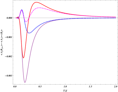
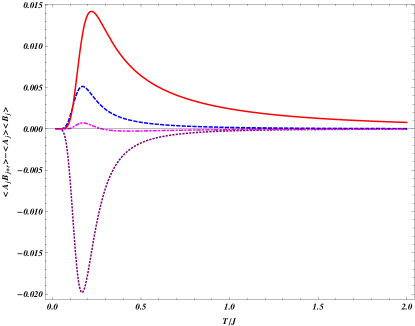
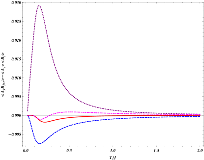
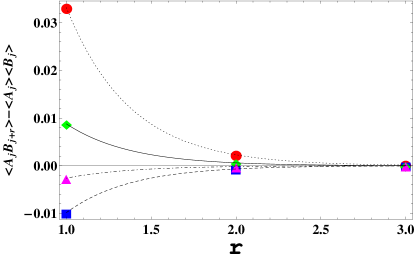
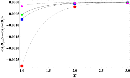
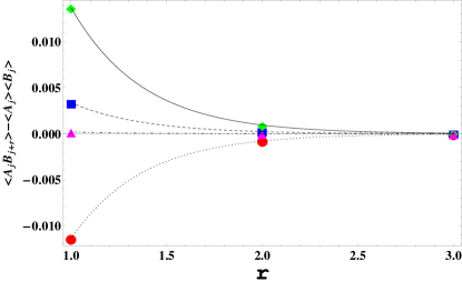
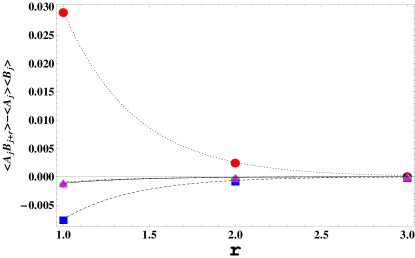
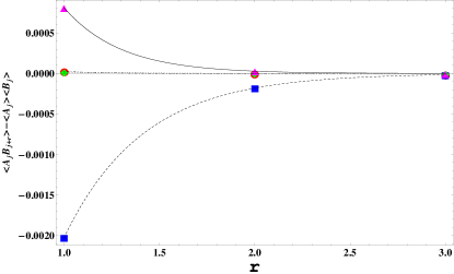
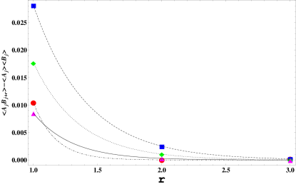
However, the thermal fluctuations as well as the effect of the magnetic field lead to non-zero correlations within a narrow interval of low temperatures for short distances. The plots of the temperature dependence of all correlation functions for the asymmetric sawtooth chain are presented in Figure 3 for the distance equal to one block, r=1𝑟1r=1. Here, the values of the parameters correspond to the spin-modulated zero-temperature ground state of the asymmetric Heisenberg-Ising sawtooth chainoha09 ; bel10 . It is rather expectable that the finite-temperature correlations are mostly of short range with respect to blocks, but as one block contains four spins, the non-zero, though weak, correlations even for r=1𝑟1r=1 are the non-trivial result. One can see from the plots in Figure 3 the vanishing of all correlations at high as well as at low temperatures as was mentioned above. As expected, the closer to each other are situated the spins from different blocks, the larger is the magnitude of the correlation between them. For instance, the correlation between τjsubscript𝜏𝑗\tau_{j} and Sj+1,1zsuperscriptsubscript𝑆𝑗11𝑧S_{j+1,1}^{z} at the temperature corresponding to the peak is four times larger in absolute value than the correlation between τjsubscript𝜏𝑗\tau_{j} and Sj+1,2zsuperscriptsubscript𝑆𝑗12𝑧S_{j+1,2}^{z} and more that seventy times larger than the correlation between Sj,2zsuperscriptsubscript𝑆𝑗2𝑧S_{j,2}^{z} and τj+1subscript𝜏𝑗1\tau_{j+1}. In the same time, the correlation between Sj,1zsuperscriptsubscript𝑆𝑗1𝑧S_{j,1}^{z} are the strongest ones, though, the are separated by The dependence of the correlation functions against the distance for the same values of coupling constants and anisotropy and for temperatures corresponding to the strongest correlation of the thermal fluctuations are presented in Figure 4. For all correlation functions one can see the usual exponential decay in their absolute value. The sign of the correlations is defined by the mutual orientation of the corresponding spins which can be seen in the T=0𝑇0T=0 ground stateoha09 ; bel10 for the given set of the parameters. In Figure 5 we presented the plots of the same correlation functions Sj,1zτj+rSj,1zτjdelimited-⟨⟩superscriptsubscript𝑆𝑗1𝑧subscript𝜏𝑗𝑟delimited-⟨⟩superscriptsubscript𝑆𝑗1𝑧delimited-⟨⟩subscript𝜏𝑗\langle S_{j,1}^{z}\tau_{j+r}\rangle-\langle S_{j,1}^{z}\rangle\langle\tau_{j}\rangle and τjSj+r,1zSj,1zτjdelimited-⟨⟩subscript𝜏𝑗superscriptsubscript𝑆𝑗𝑟1𝑧delimited-⟨⟩superscriptsubscript𝑆𝑗1𝑧delimited-⟨⟩subscript𝜏𝑗\langle\tau_{j}S_{j+r,1}^{z}\rangle-\langle S_{j,1}^{z}\rangle\langle\tau_{j}\rangle against the distance for different temperatures. The non-monotonous behavior of the correlation functions described above can be clearly seen from the plots.

V Conclusion

In the present paper we elaborated a technique for calculating correlation functions in HIC. The technique is based on the classical transfer-matrix formalism which proves itself as the most efficient and straightforward method of treating the HIC, allowing one to obtain exact expressions for the partition function and, thus, for all thermodynamic functions in a quite simple wayval08 ; ant09 ; oha09 ; oha10 ; bel10 ; roj11a ; roj11b ; lis11a ; lis11b ; oha12 ; cha12 ; roj12a ; ana12 ; roj12b . However, the classical transfer-matrix formalism is also very convenient for the calculation of the correlation functions of various kinds, because all canonical expectation values are expressed in terms of traces of certain products of the transfer-matrices with matrices representing the microscopic variables in the transfer-matrix formalismbax . We presented a detailed scheme of calculation of the correlation functions for HIC, obtained general expressions for the corresponding trace formulas and presented the general expressions for the matrix representations of the main microscopic variables for the typical HIC, quantum spin operators, additional classical spins from block Hamiltonians and intermediate spin. As it is expected from general principles, the spatial decay of any correlation between any pair of spin is characterized by a single correlation length obtained in a standard way as the reciprocal of the logarithm of the ratio of the largest and second largest eigenvalues of the classical transfer matrix. In the simplest case considered here when intermediate classical σ𝜎\sigma-spins are 1/2 spins the transfer matrix has dimension 2 by 2 and, thus, only two eigenvalues. However, the prefactors are strongly affected by the microscopic variables. We illustrated our general formalism by two examples, the simplest HIC, symmetric Heisenberg-Ising diamond-chain and asymmetric Heisenberg-Ising sawtooth chain with a pair of quantum spins in the unit cell. We presented the exact form of the transfer-matrix, its eigenvalues, matrix representation corresponding to the classical transfer-matrix formalism for quantum spin operators, matrix representation for additional classical spin from block Hamiltonian and all possible pair correlation functions. A very important feature of the correlations function of the HIC considered in the present paper is the absence of correlations between transverse components of quantum spins from different blocks. The corresponding matrix representation of the Sn,1xsuperscriptsubscript𝑆𝑛1𝑥S_{n,1}^{x} and Sn,aysuperscriptsubscript𝑆𝑛𝑎𝑦S_{n,a}^{y} operators are identically zero. This fact is an obvious consequence of the structure of the HIC where blocks interact to each other only through z𝑧z-components of the spins.

It is also worth mentioning that the general idea of using the classical transfer-matrix for describing the thermodynamic properties of decorated spin lattices can be applied also for two-dimensional systems. Although the existing examples of the papers devoted to the topic deal with the decoration-iteration transformationfisher ; str10c ; 2d1 ; 2d2 ; 2d3 ; 2d4 , the direct generalization of the existing transfer-matrix method is possible. As known, two-dimensional systems can exhibit phase transitions at finite temperature in contrast to the one-dimensional models where only zero-temperature transitions are possible. In principle, two-dimensional spin systems can possess a complicated structure of the order parameters, and multiple orderings, which, particularly, can be different in different spatial directions. For these reasons, the statement about the unique correlation length is no longer valid here.
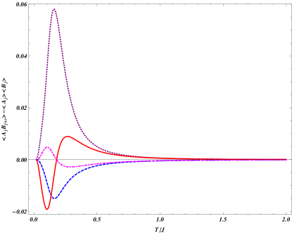
Refer to caption Refer to caption
Figure 3: (Color online) The temperature dependence of the correlation functions for the asymmetric sawtooth chain for K/J=0.5,H/J=0.5,Δ=0.3formulae-sequence𝐾𝐽0.5formulae-sequence𝐻𝐽0.5Δ0.3K/J=0.5,H/J=0.5,\Delta=0.3 at r=1𝑟1r=1 (See Eq. 54). Upper left panel: Sj,1zSj+r,1zSj,1z2delimited-⟨⟩superscriptsubscript𝑆𝑗1𝑧superscriptsubscript𝑆𝑗𝑟1𝑧superscriptdelimited-⟨⟩superscriptsubscript𝑆𝑗1𝑧2\langle S_{j,1}^{z}S_{j+r,1}^{z}\rangle-\langle S_{j,1}^{z}\rangle^{2} - dotted (purple); Sj,1zSj+r,2zSj,1zSj,2zdelimited-⟨⟩superscriptsubscript𝑆𝑗1𝑧superscriptsubscript𝑆𝑗𝑟2𝑧delimited-⟨⟩superscriptsubscript𝑆𝑗1𝑧delimited-⟨⟩superscriptsubscript𝑆𝑗2𝑧\langle S_{j,1}^{z}S_{j+r,2}^{z}\rangle-\langle S_{j,1}^{z}\rangle\langle S_{j,2}^{z}\rangle - dashed (blue); Sj,2zSj+r,1zSj,1zSj,2zdelimited-⟨⟩superscriptsubscript𝑆𝑗2𝑧superscriptsubscript𝑆𝑗𝑟1𝑧delimited-⟨⟩superscriptsubscript𝑆𝑗1𝑧delimited-⟨⟩superscriptsubscript𝑆𝑗2𝑧\langle S_{j,2}^{z}S_{j+r,1}^{z}\rangle-\langle S_{j,1}^{z}\rangle\langle S_{j,2}^{z}\rangle - solid (red); Sj,2zSj+r,2zSj,2z2delimited-⟨⟩superscriptsubscript𝑆𝑗2𝑧superscriptsubscript𝑆𝑗𝑟2𝑧superscriptdelimited-⟨⟩superscriptsubscript𝑆𝑗2𝑧2\langle S_{j,2}^{z}S_{j+r,2}^{z}\rangle-\langle S_{j,2}^{z}\rangle^{2} - dot-dashed (magenta). Upper right panel: Sj,1zσj+rSj,1zσjdelimited-⟨⟩superscriptsubscript𝑆𝑗1𝑧subscript𝜎𝑗𝑟delimited-⟨⟩superscriptsubscript𝑆𝑗1𝑧delimited-⟨⟩subscript𝜎𝑗\langle S_{j,1}^{z}\sigma_{j+r}\rangle-\langle S_{j,1}^{z}\rangle\langle\sigma_{j}\rangle - dotted (purple); Sj,2zσj+rSj,2zσjdelimited-⟨⟩superscriptsubscript𝑆𝑗2𝑧subscript𝜎𝑗𝑟delimited-⟨⟩superscriptsubscript𝑆𝑗2𝑧delimited-⟨⟩subscript𝜎𝑗\langle S_{j,2}^{z}\sigma_{j+r}\rangle-\langle S_{j,2}^{z}\rangle\langle\sigma_{j}\rangle - dashed (blue); Sj,1zτj+rSj,1zτjdelimited-⟨⟩superscriptsubscript𝑆𝑗1𝑧subscript𝜏𝑗𝑟delimited-⟨⟩superscriptsubscript𝑆𝑗1𝑧delimited-⟨⟩subscript𝜏𝑗\langle S_{j,1}^{z}\tau_{j+r}\rangle-\langle S_{j,1}^{z}\rangle\langle\tau_{j}\rangle - solid (red); Sj,2zτj+rSj,2zτjdelimited-⟨⟩superscriptsubscript𝑆𝑗2𝑧subscript𝜏𝑗𝑟delimited-⟨⟩superscriptsubscript𝑆𝑗2𝑧delimited-⟨⟩subscript𝜏𝑗\langle S_{j,2}^{z}\tau_{j+r}\rangle-\langle S_{j,2}^{z}\rangle\langle\tau_{j}\rangle - dot dashed (magenta). Lower left panel: σjSj+r,1zSj,1zσjdelimited-⟨⟩subscript𝜎𝑗superscriptsubscript𝑆𝑗𝑟1𝑧delimited-⟨⟩superscriptsubscript𝑆𝑗1𝑧delimited-⟨⟩subscript𝜎𝑗\langle\sigma_{j}S_{j+r,1}^{z}\rangle-\langle S_{j,1}^{z}\rangle\langle\sigma_{j}\rangle - dotted (purple), σjSj+r,2zSj,2zσjdelimited-⟨⟩subscript𝜎𝑗superscriptsubscript𝑆𝑗𝑟2𝑧delimited-⟨⟩superscriptsubscript𝑆𝑗2𝑧delimited-⟨⟩subscript𝜎𝑗\langle\sigma_{j}S_{j+r,2}^{z}\rangle-\langle S_{j,2}^{z}\rangle\langle\sigma_{j}\rangle - dashed (blue), σjσj+r,1zσj2delimited-⟨⟩subscript𝜎𝑗superscriptsubscript𝜎𝑗𝑟1𝑧superscriptdelimited-⟨⟩subscript𝜎𝑗2\langle\sigma_{j}\sigma_{j+r,1}^{z}\rangle-\langle\sigma_{j}\rangle^{2} - solid (red); σjτj+r,1zσjτjdelimited-⟨⟩subscript𝜎𝑗superscriptsubscript𝜏𝑗𝑟1𝑧delimited-⟨⟩subscript𝜎𝑗delimited-⟨⟩subscript𝜏𝑗\langle\sigma_{j}\tau_{j+r,1}^{z}\rangle-\langle\sigma_{j}\rangle\langle\tau_{j}\rangle - dot-dashed (magenta). Lower right panel: τjSj+r,1zSj,1zτjdelimited-⟨⟩subscript𝜏𝑗superscriptsubscript𝑆𝑗𝑟1𝑧delimited-⟨⟩superscriptsubscript𝑆𝑗1𝑧delimited-⟨⟩subscript𝜏𝑗\langle\tau_{j}S_{j+r,1}^{z}\rangle-\langle S_{j,1}^{z}\rangle\langle\tau_{j}\rangle - dotted (purple); τjSj+r,2zSj,2zτjdelimited-⟨⟩subscript𝜏𝑗superscriptsubscript𝑆𝑗𝑟2𝑧delimited-⟨⟩superscriptsubscript𝑆𝑗2𝑧delimited-⟨⟩subscript𝜏𝑗\langle\tau_{j}S_{j+r,2}^{z}\rangle-\langle S_{j,2}^{z}\rangle\langle\tau_{j}\rangle - dashed (blue); τjσj+rzσjτjdelimited-⟨⟩subscript𝜏𝑗superscriptsubscript𝜎𝑗𝑟𝑧delimited-⟨⟩subscript𝜎𝑗delimited-⟨⟩subscript𝜏𝑗\langle\tau_{j}\sigma_{j+r}^{z}\rangle-\langle\sigma_{j}\rangle\langle\tau_{j}\rangle - solid (red); τjτj+rτj2delimited-⟨⟩subscript𝜏𝑗subscript𝜏𝑗𝑟superscriptdelimited-⟨⟩subscript𝜏𝑗2\langle\tau_{j}\tau_{j+r}\rangle-\langle\tau_{j}\rangle^{2} - dot-dashed (magenta).
Refer to caption Refer to caption
Figure 4: (Color online) The dependence of the correlation functions for the asymmetric sawtooth chain against the distance for K/J=0.5,H/J=0.5,Δ=0.3formulae-sequence𝐾𝐽0.5formulae-sequence𝐻𝐽0.5Δ0.3K/J=0.5,H/J=0.5,\Delta=0.3 at r=1𝑟1r=1,222 and 333 (See Eq. 54) The lines are just the guides for the eyes. Upper left panel: T/J=0.25𝑇𝐽0.25T/J=0.25, Sj,1zSj+r,1zSj,1z2delimited-⟨⟩superscriptsubscript𝑆𝑗1𝑧superscriptsubscript𝑆𝑗𝑟1𝑧superscriptdelimited-⟨⟩superscriptsubscript𝑆𝑗1𝑧2\langle S_{j,1}^{z}S_{j+r,1}^{z}\rangle-\langle S_{j,1}^{z}\rangle^{2} - red circles (dotted); Sj,1zSj+r,2zSj,1zSj,2zdelimited-⟨⟩superscriptsubscript𝑆𝑗1𝑧superscriptsubscript𝑆𝑗𝑟2𝑧delimited-⟨⟩superscriptsubscript𝑆𝑗1𝑧delimited-⟨⟩superscriptsubscript𝑆𝑗2𝑧\langle S_{j,1}^{z}S_{j+r,2}^{z}\rangle-\langle S_{j,1}^{z}\rangle\langle S_{j,2}^{z}\rangle - blue squares (dashed); Sj,2zSj+r,1zSj,1zSj,2zdelimited-⟨⟩superscriptsubscript𝑆𝑗2𝑧superscriptsubscript𝑆𝑗𝑟1𝑧delimited-⟨⟩superscriptsubscript𝑆𝑗1𝑧delimited-⟨⟩superscriptsubscript𝑆𝑗2𝑧\langle S_{j,2}^{z}S_{j+r,1}^{z}\rangle-\langle S_{j,1}^{z}\rangle\langle S_{j,2}^{z}\rangle - green diamonds (solid); Sj,2zSj+r,2zSj,2z2delimited-⟨⟩superscriptsubscript𝑆𝑗2𝑧superscriptsubscript𝑆𝑗𝑟2𝑧superscriptdelimited-⟨⟩superscriptsubscript𝑆𝑗2𝑧2\langle S_{j,2}^{z}S_{j+r,2}^{z}\rangle-\langle S_{j,2}^{z}\rangle^{2} - magenta triangles (dot-dashed). Upper right panel: T/J=0.25𝑇𝐽0.25T/J=0.25, Sj,1zσj+rSj,1zσjdelimited-⟨⟩superscriptsubscript𝑆𝑗1𝑧subscript𝜎𝑗𝑟delimited-⟨⟩superscriptsubscript𝑆𝑗1𝑧delimited-⟨⟩subscript𝜎𝑗\langle S_{j,1}^{z}\sigma_{j+r}\rangle-\langle S_{j,1}^{z}\rangle\langle\sigma_{j}\rangle - red circles (dotted); Sj,2zσj+rSj,2zσjdelimited-⟨⟩superscriptsubscript𝑆𝑗2𝑧subscript𝜎𝑗𝑟delimited-⟨⟩superscriptsubscript𝑆𝑗2𝑧delimited-⟨⟩subscript𝜎𝑗\langle S_{j,2}^{z}\sigma_{j+r}\rangle-\langle S_{j,2}^{z}\rangle\langle\sigma_{j}\rangle - blue squares (dashed); Sj,1zτj+rSj,1zτjdelimited-⟨⟩superscriptsubscript𝑆𝑗1𝑧subscript𝜏𝑗𝑟delimited-⟨⟩superscriptsubscript𝑆𝑗1𝑧delimited-⟨⟩subscript𝜏𝑗\langle S_{j,1}^{z}\tau_{j+r}\rangle-\langle S_{j,1}^{z}\rangle\langle\tau_{j}\rangle - green diamonds (solid); Sj,2zτj+rSj,2zτjdelimited-⟨⟩superscriptsubscript𝑆𝑗2𝑧subscript𝜏𝑗𝑟delimited-⟨⟩superscriptsubscript𝑆𝑗2𝑧delimited-⟨⟩subscript𝜏𝑗\langle S_{j,2}^{z}\tau_{j+r}\rangle-\langle S_{j,2}^{z}\rangle\langle\tau_{j}\rangle - magenta triangles (dot-dashed). Lower left panel: T/J=0.25𝑇𝐽0.25T/J=0.25, σjSj+r,1zSj,1zσjdelimited-⟨⟩subscript𝜎𝑗superscriptsubscript𝑆𝑗𝑟1𝑧delimited-⟨⟩superscriptsubscript𝑆𝑗1𝑧delimited-⟨⟩subscript𝜎𝑗\langle\sigma_{j}S_{j+r,1}^{z}\rangle-\langle S_{j,1}^{z}\rangle\langle\sigma_{j}\rangle - red circles (dotted), σjSj+r,2zSj,2zσjdelimited-⟨⟩subscript𝜎𝑗superscriptsubscript𝑆𝑗𝑟2𝑧delimited-⟨⟩superscriptsubscript𝑆𝑗2𝑧delimited-⟨⟩subscript𝜎𝑗\langle\sigma_{j}S_{j+r,2}^{z}\rangle-\langle S_{j,2}^{z}\rangle\langle\sigma_{j}\rangle - blue squares (dashed), σjσj+r,1σj2delimited-⟨⟩subscript𝜎𝑗subscript𝜎𝑗𝑟1superscriptdelimited-⟨⟩subscript𝜎𝑗2\langle\sigma_{j}\sigma_{j+r,1}\rangle-\langle\sigma_{j}\rangle^{2} - green diamonds (solid); σjτj+r,1σjτjdelimited-⟨⟩subscript𝜎𝑗subscript𝜏𝑗𝑟1delimited-⟨⟩subscript𝜎𝑗delimited-⟨⟩subscript𝜏𝑗\langle\sigma_{j}\tau_{j+r,1}\rangle-\langle\sigma_{j}\rangle\langle\tau_{j}\rangle - magenta triangles (dot-dashed). Lower right panel: T/J=0.15𝑇𝐽0.15T/J=0.15, τjSj+r,1zSj,1zτjdelimited-⟨⟩subscript𝜏𝑗superscriptsubscript𝑆𝑗𝑟1𝑧delimited-⟨⟩superscriptsubscript𝑆𝑗1𝑧delimited-⟨⟩subscript𝜏𝑗\langle\tau_{j}S_{j+r,1}^{z}\rangle-\langle S_{j,1}^{z}\rangle\langle\tau_{j}\rangle - red circles (dotted); τjSj+r,2zSj,2zτjdelimited-⟨⟩subscript𝜏𝑗superscriptsubscript𝑆𝑗𝑟2𝑧delimited-⟨⟩superscriptsubscript𝑆𝑗2𝑧delimited-⟨⟩subscript𝜏𝑗\langle\tau_{j}S_{j+r,2}^{z}\rangle-\langle S_{j,2}^{z}\rangle\langle\tau_{j}\rangle - blue squares (dashed); τjσj+rσjτjdelimited-⟨⟩subscript𝜏𝑗subscript𝜎𝑗𝑟delimited-⟨⟩subscript𝜎𝑗delimited-⟨⟩subscript𝜏𝑗\langle\tau_{j}\sigma_{j+r}\rangle-\langle\sigma_{j}\rangle\langle\tau_{j}\rangle - green diamonds (solid); τjτj+rτj2delimited-⟨⟩subscript𝜏𝑗subscript𝜏𝑗𝑟superscriptdelimited-⟨⟩subscript𝜏𝑗2\langle\tau_{j}\tau_{j+r}\rangle-\langle\tau_{j}\rangle^{2} - magenta triangles (dot-dashed).
Refer to caption Refer to caption
Figure 5: (Color online) The dependence of the correlation functions Sj,1zτj+rSj,1zτjdelimited-⟨⟩superscriptsubscript𝑆𝑗1𝑧subscript𝜏𝑗𝑟delimited-⟨⟩superscriptsubscript𝑆𝑗1𝑧delimited-⟨⟩subscript𝜏𝑗\langle S_{j,1}^{z}\tau_{j+r}\rangle-\langle S_{j,1}^{z}\rangle\langle\tau_{j}\rangle (left panel) and τjSj+r,1zSj,1zτjdelimited-⟨⟩subscript𝜏𝑗superscriptsubscript𝑆𝑗𝑟1𝑧delimited-⟨⟩superscriptsubscript𝑆𝑗1𝑧delimited-⟨⟩subscript𝜏𝑗\langle\tau_{j}S_{j+r,1}^{z}\rangle-\langle S_{j,1}^{z}\rangle\langle\tau_{j}\rangle (right panel) against the distance for different temperatures at r=1𝑟1r=1, 222 and 333. The lines are just the guides for the eyes. T/J=0.05𝑇𝐽0.05T/J=0.05 - red bullets (dot-dashed ); T/J=0.18𝑇𝐽0.18T/J=0.18 - blue squares (dashed); T/J=0.28𝑇𝐽0.28T/J=0.28 - green diamonds (dotted); T/J=0.42𝑇𝐽0.42T/J=0.42 - magenta triangles (solid).

VI Acknowledgements

V.O. expresses his gratitude to the LNF-INFN in Frascati for warm hospitality during the work on the paper. He also acknowledges partial financial support from Volkswagen Foundation (Grant No. I/84 496) and from the project SCS-BFBR 11RB-001.

References

  • (1) J. Strečka and M. Jaščur, J. Phys.: Condens. Matter 15, 4519 (2003).
  • (2) J. Strečka, M. Hagiwara, M. Jaščur, and K. Minami, Czech. J. Phys. 54, D583 (2004).
  • (3) J. Strečka, M. Jaščur, M. Hagiwara, Y. Narumi, and K. Kindo, K. Minami, Phys. Rev. B 72, 024459 (2005).
  • (4) L. Čanová, J. Strečka and M. Jaščur, J. Phys. : Condens. Matter 18, 4967 (2006).
  • (5) J. S. Valverde, O. Rojas, and S. M. de Souza, J. Phys.: Condens. Matter 20, 345208 (2008).
  • (6) M. S. S. Pereira, F. A. B. F. de Moura, and M. L. Lyra, Phys. Rev. B 77, 024402 (2008).
  • (7) M. S. S. Pereira, F. A. B. F. de Moura, and M. L. Lyra, Phys. Rev. B 79, 054427 (2009).
  • (8) J. Strečka, L. Čanová, T. Lučivjanský, and M. Jaščur, J. Phys.: Conf. Ser. 145, 012058 (2009).
  • (9) D. Antonosyan, S. Bellucci, and V. Ohanyan, Phys. Rev. B 79, 014432 (2009).
  • (10) V. Ohanyan, Condens. Matter Phys. 12, 343 (2009).
  • (11) V. Ohanyan, Phys. Atomic Nucl. 73, 494 (2010).
  • (12) J. Strečka, L. Galisova, and O. Derzhko, Acta Phys. Pol. A 118, 742 (2010).
  • (13) S. Bellucci and V. Ohanyan, Eur. Phys. J. B 75, 531 (2010).
  • (14) O. Rojas, S. M. de Souza, V. Ohanyan, and M. Khurshudyan, Phys. Rev. B 83, 094430 (2011).
  • (15) O. Rojas and S. M. de Souza, Phys. Lett. A 375, 1295 (2011).
  • (16) B. Lisnii, Low Temp. Phys. 37, 296 (2011).
  • (17) B. Lisnii, Ukr. Journal of Phys. 56, 1237 (2011).
  • (18) J. Strečka, M.Dančo, Physica B 406, 2967 (2011).
  • (19) V. Ohanyan and A. Honecker, Phys. Rev. B 86, 054412 (2012).
  • (20) L. Chakhmakhchyan, N. Ananikian, L. Ananikyan, and Č. Burdik, J. Phys.: Conf. Ser. 343, 012022 (2012).
  • (21) O. Rojas, S. M. de Souza, and N. S. Ananikian, Phys. Rev. E 85, 061123 (2012).
  • (22) N. Ananikian, L. Ananikyan, L. Chakhmakhchyan, and O. Rojas, J. Phys.: Condens. Matter 24, 256001 (2012).
  • (23) T. Verkholyak, J. Strečka, J.Phys. A: Mathematical and Theoretical, 45, 305001 (2012).
  • (24) J. Strečka, M. Hagiwara, Y. Han, T. Kida, Z. Honda, and M. Ikeda, Condens. Matter Phys. 15, 43002 (2012).
  • (25) L. Galisova, phys. stat. solidi(b) 250, 187 (2013).
  • (26) O. Rojas, M. Rojas, N. S. Ananikian and S. M. de Souza, Phys. Rev. A 86, 042330 (2012).
  • (27) R. Baxter, Exactly Solved Models in Statistical Mechanics, (Academic Press, New York, 1982).
  • (28) V. Ohanyan and N. Ananikian, Phys. Lett. A 307, 76 (2003).
  • (29) E. Aydiner and C. Akyüz, Chin. Phys. Lett. 22, 2382 (2005).
  • (30) E. Aydiner, C. Akyüz, M. Gönülol, and H. Polat, phys. stat. sol(b) 243, 2901 (2006).
  • (31) D. Gatteschi, R. Sessoli, and J. Villain, Molecular Nanomagnets (Oxford Univ. PRess, New York 2007).
  • (32) D. Visinescu, A. M. Madalan, M. Andruh, C. Duhayon, J.-P. Sutter, L. Ungur, W. Van den Heuvel, and L. F. Chibotaru, Chem. Eur. J. 15, 11808 (2009).
  • (33) J. Rinck, G. Novitchi, W. Van den Heuvel, L. Ungur, Y. Lan, W. Wernsdorfer, C. E. Anson, L. F. Chibotaru, and A. K. Powell, Angew. Chem., Int. Ed. 49, 7583 (2010).
  • (34) W. Van den Heuvel and L. F. Chibotaru, Phys. Rev. B 82, 174436 (2010).
  • (35) V. Ravi Chandra, S. Ramasesha, and D. Sen, Phys. Rev. B 70, 144404 (2004).
  • (36) T. S. Venkatakrishnan, S. Sahoo, Nicolas Bréfuel, C. Duhayon, C. Paulsen, A.-L. Barra, S. Ramasesha, and J.-P. Sutter, J. Am. Chem. Soc. 132, 6047 (2010).
  • (37) S. Sahoo, J.-P. Sutter, and S. Ramasesha, J. Stat. Phys. 147, 181 (2012).
  • (38) M. E. Fisher, Phys. Rev. 113, 969 (1959).
  • (39) O. Rojas, J. S. Valverde and S. M.  de Souza, Physica A 388, 1419 (2009).
  • (40) J. Strečka, Phys. Lett. A 374, 3718 (2010).
  • (41) M. Knežević and S. Milošević, J. Phys. A: Math. Gen. 13, 2479 (1980).
  • (42) R. J. V. dos Santos and M. L. Lyra, Physica A 182, 133 (1992).
  • (43) J. Strečka, L. Čanová, and K. Minami, Phys. Rev. B 79, 051103 (2009).
  • (44) J. Strečka, O. Rojas, and S. M. de Souza, Eur. Phys. J. B 85, 54 (2010).
  • (45) J.Čiśarova, and J. Strečka, Phys. Rev. B 87, 024421 (2013).
  • (46) J.Čiśarova, F. Michaud, F. Mila, and J. Strečka, Phys. Rev. B 87, 054419 (2013).