Discrete holomorphicity and Ising model operator formalism

Abstract.

We explore the connection between the transfer matrix formalism and discrete complex analysis approach to the two dimensional Ising model.

We construct a discrete analytic continuation matrix, analyze its spectrum and establish a direct connection with the critical Ising transfer matrix. We show that the lattice fermion operators of the transfer matrix formalism satisfy, as operators, discrete holomorphicity, and we show that their correlation functions are Ising parafermionic observables. We extend these correspondences also to outside the critical point.

We show that critical Ising correlations can be computed with operators on discrete Cauchy data spaces, which encode the geometry and operator insertions in a manner analogous to the quantum states in the transfer matrix formalism.

1. Introduction

The transfer matrix approach to the planar Ising model is both classical and remarkably powerful [KrWa41, Bax82, McWu73]. The free energy, critical exponents and a number of correlation functions of the model were calculated using the transfer matrix, and much of the algebraic structure underlying the model is easiest understood by means of the transfer matrix and the related operator formalism. The formalism is also manifestly suggestive of the quantum field theories believed to describe the scaling limit of the Ising model.

Recently, methods of discrete complex analysis have lead to significant progress in the understanding of the Ising model, especially in its critical phase [Smi06, Smi10b]. The discrete complex analysis techniques apply to the model on planar domains of arbitrary shapes, and allow to prove conformal invariance results.

In this paper, we investigate connections between the transfer matrix approach and discrete complex analysis techniques. We study discrete level relations between the two approaches, using concepts of quantum field theory and analytic tools that are well behaved in the scaling limit.

1.1. Ising model

The Ising model describes up/down spins interacting on a lattice. It is a simple model originally introduced to describe ferromagnetism, but subsequently it has become a standard in the study of order-disorder phase transition.

The Ising model is a random assignment of $\pm 1$ spins to the vertices a graph, that interact via the edges of the graph. We will consider the Ising model on subgraphs $\mathcal{G}=(\mathcal{V},\mathcal{E})$ of the square lattice $\mathbb{Z}^{2}$.

The probability of a spin configuration $\left(\mathbf{s}_{x}\right)_{x\in\mathcal{V}}$ is proportional to the Boltzmann weight $e^{-\beta H\left(\mathbf{s}\right)}$, where $\beta>0$ is the inverse temperature and $H$ is the energy given by $H(\mathbf{s})=-\sum_{i\sim j}\mathbf{s}_{i}\mathbf{s}_{j}$ with sum over pairs of adjacent vertices $<i,j>\in\mathcal{E}$. Hence, the model favors local alignment of spins by assigning them a lower energy, and the strength of this effect is controlled by $\beta$.

For the Ising model in dimensions at least two, a phase transition in the large scale behavior occurs at a critical inverse temperature, for the square lattice Ising model at $\beta_{c}=\frac{1}{2}\ln\left(\sqrt{2}+1\right)$. For $\beta<\beta_{c}$, the system is disordered: spins at large distances decorrelate, i.e. there is no alignment. For $\beta>\beta_{c}$ the system has long-range order: spins are uniformly positively correlated, i.e. global alignment takes place. To properly make sense of the large scale behavior, one considers either the thermodynamic limit in which the graph tends to the infinite square lattice $\mathcal{G}\nearrow\mathbb{Z}^{2}$, or the scaling limit in which a given planar domain $\Omega$ is approximated by subgraphs $\Omega_{\delta}$ of $\delta\mathbb{Z}^{2}$, the square lattice with fine lattice mesh $\delta\searrow 0$.

The square-lattice Ising model is exactly solvable: in particular, the free energy and thermodynamical properties of the model are well understood. However, the fine nature of the critical phase and its precise connection with quantum field theory have for long remained mysterious from a mathematical perspective. Renormalization group and quantum field theory methods have provided a non-rigorous insight into the nature of the phase transition, Conformal Field Theory in particular giving numerous exact predictions. At the critical point, $\beta=\beta_{c}$, the model (like many critical two dimensional lattice models) should have a universal, conformally invariant scaling limit. Recently some of this insight has become tractable mathematically by the development of discrete complex analysis techniques: one can make sense of the scaling limits of the fields and the curves of the model at the critical temperature.

• The scaling limits of the random fields of the model are described by a Conformal Field Theory. The CFTs are quantum field theories with infinite-dimensional symmetries, which allow one to compute the critical exponents and the correlation functions via representation theoretic methods [BPZ84a, BPZ84b].

• The scaling limits of the random curves of the model are described by a Schramm-Loewner Evolution. The SLEs are random processes characterized by their conformal invariance and a Markovian property with respect to the domain [Sch00].

A natural framework to investigate full conformal invariance of the Ising model (and other models) is to study the model on arbitrary planar domains, with boundary conditions. A number of results in this framework has been obtained in recent years: the convergence in the scaling limit has been shown for parafermionic observables [Smi06, Smi10a, ChSm09], for the energy correlations [HoSm10b, Hon10a] and for the spin correlations [ChIz11, CHI12]. These scaling limit results for correlations rely, for a large part, on discrete complex analysis. They have in turn provided the key tools to identify and control convergence of the random curves in the scaling limit [Smi06, CDHKS12, HoKy11].

In the special case of the full plane, the progress in the study of scaling limits of Ising model at and near criticality has been steady over a longer time. In notable results, massive correlations in the full plane have been computed [WMTB76] and formulated in terms of holonomic field theory [SMJ77, SMJ79a, SMJ79b, SMJ80, PaTr83, Pal07]. Critical correlations in the full plane have been computed using dimer techniques and discrete analysis [BoDT09, BoDT08, Dub11a, Dub11b].

1.2. Transfer matrix and discrete holomorphicity

In this subsection, we briefly introduce the two approaches to the Ising model studied in this paper: the transfer matrix and the discrete complex analysis formalisms.

1.2.1. Transfer matrix approach

Let $\mathbf{I}$ be an interval of $\mathbb{Z}$, with boundary $\partial\mathbf{I}\subset\mathbf{I}$ consisting of the two endpoints of the interval, and consider the rectangular box $\mathbf{I}\times\left\{0,\ldots,N\right\}$ with rows $\mathbf{I}_{0},\ldots,\mathbf{I}_{N}$ (set $\mathbf{I}_{y}:=\mathbf{I}\times\left\{y\right\}$). Using the transfer matrix, we can represent the Ising model on $\mathbf{I}\times\left\{0,\ldots,N\right\}$ as a quantum evolution of spins living on $\mathbf{I}$ from time $0$ to time $N$.

The Ising model transfer matrix $V$ acts on a state space $\mathcal{S}$, which has basis $(\mathbf{e}_{\sigma}$) indexed by spin configurations in a row, $\sigma\in\left\{\pm 1\right\}^{\mathbf{I}}$. We set $V:=\left(V^{\mathrm{h}}\right)^{\frac{1}{2}}V^{\mathrm{v}}\left(V^{\mathrm{h}}\right)^{\frac{1}{2}}$, where the factors separately account for Ising interactions along horizontal and vertical edges. The matrix element of $V^{\mathrm{v}}$ at $\sigma,\rho\in\left\{\pm 1\right\}^{\mathbf{I}}$ is defined (with fixed boundary conditions) as

$$V_{\sigma\rho}^{\mathrm{v}}=\begin{cases}\exp\left(\beta\sum_{i\in\mathbf{I}}\sigma_{i}\rho_{i}\right)&\mbox{ if }\sigma|_{\partial\mathbf{I}}=\rho|_{\partial\mathbf{I}}\\ 0&\mbox{otherwise}\end{cases}$$

and the matrix $V^{\mathrm{h}}$ is diagonal with elements

$$V_{\sigma\sigma}^{\mathrm{h}}=\exp\left(\beta\sum_{x\sim y}\sigma_{x}\sigma_{y}\right).$$

Viewing the $y$-axis as time, the transfer matrix can be thought of as an exponentiated quantum Hamiltonian in $1+1$ dimensional space-time: at the row $\mathbf{I}_{y}$, we have a quantum state $\mathbf{v}_{y}\in\mathcal{S}$ which we propagate to the next row $\mathbf{I}_{y+1}$ by $\mathbf{v}_{y+1}=V\mathbf{v}_{y}$.

In the path integral picture, the evolution $\mathbf{v}_{0},\ldots,\mathbf{v}_{N}$ becomes a sum over trajectories weighted by their amplitudes: the trajectories are spin configurations $\mathbf{s}:\mathbf{I}\times\left\{0,\ldots,N\right\}\to\left\{\pm 1\right\}$ and the amplitudes are the Boltzmann weights $e^{-\beta H\left(\mathbf{s}\right)}$. As a result, the partition function $Z=\sum_{\mathbf{s}}e^{-\beta H\left(\mathbf{s}\right)}$ equals $\left\langle\mathbf{f}|V^{N}|\mathbf{i}\right\rangle:=\mathbf{f}^{\top}V^{N}\mathbf{i}$, where $\mathbf{i},\mathbf{f}\in\mathcal{S}$ encode the boundary conditions on $\mathbf{I}_{0}$ and $\mathbf{I}_{N}$.

Ising fields (such as the spin, energy, disorder, fermions) are represented by the insertion of corresponding operators. The position of the fields appear in two ways: the operator is applied to the state on the row $y$ on which the field lives, and the applied operator $O_{x}:\mathcal{S}\to\mathcal{S}$ depends on the position $x$ of the field in that row. We combine the dependence on the horizontal coordinate $x$ and the vertical time coordinate $y$ by using the operator $O(z)=V^{-y}O_{x}V^{y}$ for the field located at $z=x+\mathfrak{i}y$. Then the correlation function of fields $O^{(1)},\ldots,O^{(n)}$ located at $z_{1},\ldots,z_{n}$ is

$$\left\langle O^{(1)}\left(z_{1}\right)\cdots O^{(n)}\left(z_{n}\right)\right\rangle=\frac{\langle\mathbf{f}|V^{N}O^{(1)}\left(z_{1}\right)\cdots O^{(n)}\left(z_{n}\right)|\mathbf{i}\rangle}{\langle\mathbf{f}|V^{N}|\mathbf{i}\rangle}.$$

For probabilistic fields such as the spin $\mathbf{s}_{z}$, represented by $\hat{\sigma}\left(z\right):\mathcal{S}\to\mathcal{S}$, the correlation functions are the expected values of products, e.g. $\left\langle\hat{\sigma}\left(z_{1}\right)\cdots\hat{\sigma}\left(z_{n}\right)\right\rangle=\mathbb{E}\left[\mathbf{s}_{z_{1}}\cdots\mathbf{s}_{z_{n}}\right]$. Non-probabilistic fields (such as fermion and disorder) can also be represented within the transfer matrix formalism.

Also in Conformal Field Theory, the field-to-operator correspondence is fundamental. However, naively connecting the algebraic structure of Ising model and the one of CFT is problematic: the transfer matrix does not have a nice scaling limit and it is best suited to very specific geometries (rectangle, cylinder, torus, plane).

Contrary to the transfer matrix formalism, discrete complex analysis is well suited to handle scaling limits on domains of arbitrary geometry, and hence to discuss conformal invariance. For this reason, relating the transfer matrix to discrete complex analysis seems a promising way to provide a manageable scaling limit for the quantum field theoretic concepts of the transfer matrix formalism.

1.2.2. Discrete complex analysis approach

The idea of discrete complex analysis is to identify fields on lattice level, whose correlations satisfy difference equations — lattice analogues of equations of motion. A particularly useful type of such equations are strong lattice Cauchy-Riemann equations (massless at $\beta_{c}$, massive at $\beta\neq\beta_{c}$), which we will refer to as ’s-holomorphicity’.

For the critical Ising model, certain s-holomorphic fields can be completely characterized in terms of discrete complex analysis: their correlation functions (called ’observables’) can be formulated as the unique solutions to discrete Riemann-type boundary value problems (RBVP). The convergence of s-holomorphic observables is in particular the main tool to establish convergence of Ising interfaces to SLE [Smi06, CDHKS12, HoKy11], and to prove conformal invariance of the energy and the spin correlations [HoSm10b, Hon10a, CHI12].

A key example is the Ising parafermionic observable of [ChSm09]. On a discrete domain $\Omega$ (finite simply connected union of faces of $\mathbb{Z}^{2}$), for two midpoints of edges $a$ and $z$, the observable is defined by

$$f\left(a,z\right)=\frac{1}{\mathcal{Z}}\sum_{\gamma:a\leadsto z}e^{-2\beta\#\mathrm{edges}\left(\gamma\right)}e^{-\frac{i}{2}\mathrm{winding}\left(\gamma:a\to z\right)},$$

where $\mathcal{Z}$ is a partition function, the sum is over collections $\gamma$ of dual edges, consisting of loops and a path from $a$ to $z$, and $\mathrm{winding}\left(\gamma:a\to z\right)$ is the total turning angle of the path.

At critical temperature $\beta=\beta_{c}$, when $a$ is a bottom horizontal boundary edge, the function $f_{a}:=f(a,\cdot)$ is the unique solution of a discrete RBVP:

• $f_{a}$ is s-holomorphic: for any two incident edges $e_{v}=\left\langle vu\right\rangle$ and $e_{w}=\left\langle wu\right\rangle$, the values of $f_{a}$ satisfy the real-linear equation $f_{a}\left(e_{v}\right)+\frac{i}{\theta}\overline{f_{a}\left(e_{v}\right)}=f_{a}\left(e_{w}\right)+\frac{i}{\theta}\overline{f_{a}\left(e_{w}\right)}$, where $\theta=\frac{2u-v-w}{\left|2u-v-w\right|}$.

• On the boundary, values of $f_{a}$ are real multiples of $\tau_{\mathrm{cw}}^{-\frac{1}{2}}$, where $\tau_{\mathrm{cw}}$ is the clockwise tangent to the boundary.

• $f_{a}$ satisfies the normalization condition $f_{a}(a)=1$.

One can then show that the solutions of discrete RBVPs converge to the solutions of continuous RBVPs, which are conformally covariant [Smi06, Smi10a, Hon10a, HoSm10b, ChSm09, ChIz11, CHI12].

The approach of s-holomorphic functions has proved succesful for the study of conformal invariance: it applies to arbitrary planar geometries, general graphs and behaves well in the scaling limit. Still, the algebraic structures of CFT are not apparent in the s-holomorphic approach: there is no Hilbert space of states, no obvious action of the Virasoro algebra and no simple reason for the continuous correlations to obey the CFT null-field PDEs. To connect the Ising model with CFT, one would like to write algebraic data (e.g. from transfer matrix) in s-holomorphic terms and then to pass to the limit.

1.3. Main results

The goal of this paper is to explore the connection between the transfer matrix formalism and s-holomorphicity approach to the critical Ising model, and to lay foundations for a quantum field theoretic description that behaves well in the scaling limit.

We construct a discrete analytic continuation matrix, analyze its spectrum and establish a direct connection with the Ising transfer matrix. We show that the lattice fermion operators of the transfer matrix formalism satisfy, as operators, s-holomorphic equations of motion, and we show that their correlation functions are s-holomorphic Ising parafermionic observables. Finally, we show that Ising correlations can be computed with lattice Poincaré-Steklov operators, which encode the geometry and operator insertions in a manner analogous to the quantum states in the transfer matrix formalism.

The results admit generalizations to non-critical Ising model, with s-holomorphicity replaced by a concept of massive s-holomorphicity.

1.3.1. Discrete analytic continuation and Ising transfer matrix

Let $a<b$ be integers, consider the interval $\mathbf{I}:=\left\{x\in\mathbb{Z}:a\leq x\leq b\right\}$ and let $\partial\mathbf{I}:=\left\{a,b\right\}$ denote its boundary. Let $\mathbf{I}^{*}$ be the dual of $\mathbf{I}$, the set of half-integers between $a$ and $b$. Write $\mathbf{I}_{0}^{*}:=\mathbf{I}^{*}\times\left\{0\right\}$, $\mathbf{I}_{\frac{1}{2}}:=\mathbf{I}\times\left\{\frac{1}{2}\right\}$, etc. For simplicity of notation, we identify edges with their midpoints.

Lemma (Section 2.4).

Let $f:\mathbf{I}_{0}^{*}\to\mathbb{C}$ be a complex-valued function. Then there is a unique s-holomorphic extension $h$ of $f$ to $\mathbf{I}_{0}^{*}\cup\mathbf{I}_{\frac{1}{2}}\cup\mathbf{I}_{1}^{*}$ with Riemann boundary values on $\partial\mathbf{I}_{\frac{1}{2}}$.

Since s-holomorphicity and RBVP are $\mathbb{R}$-linear concepts, we identify $\mathbb{C}\cong\mathbb{R}^{2}$ and denote by $P:\left(\mathbb{R}^{2}\right)^{\mathbf{I}^{*}}\to\left(\mathbb{R}^{2}\right)^{\mathbf{I}^{*}}$ the $\mathbb{R}$-linear linear map $f\mapsto h\Big{|}_{\mathbf{I}_{1}^{*}}$. In other words, $P$ is the row-to-row propagation of s-holomorphic solutions of the Riemann boundary value problem.

Proposition (Proposition 7 in Section 2.5.).

The operator $P$ can be diagonalized and has a positive spectrum, given by $\lambda_{\alpha}^{\pm 1}$ where $\lambda_{\alpha}>1$ are distinct for $\alpha=1,\ldots,\left|\mathbf{I}\right|^{*}$.

Let $P^{\mathbb{C}}:\left(\mathbb{C}^{2}\right)^{\mathbf{I}^{*}}\to\left(\mathbb{C}^{2}\right)^{\mathbf{I}^{*}}$ be the complexification of $P$, i.e. the $\mathbb{C}$-linear map such that $P^{\mathbb{C}}\big{|}_{\left(\mathbb{R}^{2}\right)^{\mathbf{I}^{*}}}=P$. Let $W_{\circ}\subset\left(\mathbb{C}^{2}\right)^{\mathbf{I}^{*}}$ be the vector space spanned by the eigenvectors of $P^{\mathbb{C}}$ of eigenvalues less than $1$ and let $P_{\circ}^{\mathbb{C}}:W_{\circ}\to W_{\circ}$ be the restriction of $P^{\mathbb{C}}$ to $W_{\circ}$.

Theorem (Theorem 18 in Section 3.3).

Let $\bigwedge W_{\circ}$ be the exterior tensor algebra $\bigoplus_{n=0}^{\left|\mathbf{I}^{*}\right|}\bigwedge^{n}W_{\circ}$ and let $\Gamma\left(P_{\circ}^{\mathbb{C}}\right):\bigwedge W_{\circ}\to\bigwedge W_{\circ}$ be defined as $\bigoplus_{n=0}^{\left|\mathbf{I}^{*}\right|}\left(P_{\circ}^{\mathbb{C}}\right)^{\otimes n}$. Let $V_{+}:\mathcal{S}_{+}\to\mathcal{S}_{+}$ be the Ising model transfer matrix at the critical point $\beta=\beta_{c}$, restricted to the subspace $\mathcal{S}_{+}\subset\mathcal{S}$ defined as $\mathrm{span}\left\{\mathbf{e}_{\sigma}:\sigma_{b}=1\right\}$ (see Section 1.2.1).

Then there is an isomorphism $\rho:\mathcal{S}_{+}\to\bigwedge\left(W_{\circ}\right)$ such that $\rho\circ V\circ\rho^{-1}=\Lambda_{0}\times\Gamma\left(P_{\circ}^{\mathbb{C}}\right)$ for some $\Lambda_{0}>0$.

It follows in particular that the spectrum of the critical Ising model transfer matrix is completely determined by the spectrum of the discrete analytic continuation matrix $P$.

1.3.2. Induced rotation and s-holomorphic propagation

The theorem of Section Theorem relies on the Kaufman representation of the Ising transfer matrix [Kau49]: $V$ can be constructed from its so-called induced rotation $T_{V}$ on a space of Clifford generators defined below. The connection with discrete analysis is made by observing that the s-holomorphic propagation $P^{\mathbb{C}}$ is actually equal (up to a change of basis) to $T_{V}$.

For $k\in\mathbf{I}^{*}$ and a spin configuration $\sigma\in\left\{\pm 1\right\}^{\mathbf{I}}$. We define the operators $p_{k}:\mathcal{S}\to\mathcal{S}$ and $q_{k}:\mathcal{S}\to\mathcal{S}$ by

$$\begin{array}[]{c}p_{k}\left(\mathbf{e}_{\sigma}\right)=\;\sigma_{k+\frac{1}{2}}\mathbf{e}_{\tau}\\ q_{k}\left(\mathbf{e}_{\sigma}\right)=\mathfrak{i}\,\sigma_{k-\frac{1}{2}}\mathbf{e}_{\tau}\end{array}\qquad\text{, where} \tau_{x}=\; \begin{cases}\phantom{-}\sigma_{x\quad}&\text{for }x>k\\ -\sigma_{x}\quad&\text{for }x<k.\end{cases}$$

Let $\mathcal{W}$ be the space of operators $\mathcal{S}\to\mathcal{S}$ spanned by $\left\{p_{k},q_{k}\,\big{|}\,k\in\mathbf{I}^{*}\right\}$. The conjugation $\mathcal{O}\mapsto V\mathcal{O}V^{-1}$ defines a linear operator $\mathcal{W}\to\mathcal{W}$, which we denote by $T_{V}$ and call the induced rotation of $V$.

Theorem (Theorem 10 in Section 3.2).

Let $T_{V}:\mathcal{W}\to\mathcal{W}$ be the induced rotation of $V$ at critical point $\beta=\beta_{c}$, and let $P^{\mathbb{C}}:\left(\mathbb{C}^{2}\right)^{\mathbf{I}^{*}}\to\left(\mathbb{C}^{2}\right)^{\mathbf{I}^{*}}$ be the complexified s-holomorphic propagation. Then there is an isomorphism $\varrho:\left(\mathbb{C}^{2}\right)^{\mathbf{I}^{*}}\to\mathcal{W}$ such that $T_{V}:=\varrho\circ P^{\mathbb{C}}\circ\varrho^{-1}$.

1.3.3. Fermion operators

An important tool for the analysis of the Ising model in the transfer matrix formalism are the fermion operators; similarly, the study of the scaling limit of the Ising model on planar domains relies on s-holomorphic parafermionic observables. We discuss two facts pertaining to the relation of these two, namely that the fermion operators are complexified s-holomorphic (as matrix-valued functions) and that their correlations are indeed the parafermionic observables discussed in Section 1.3.1.

Theorem (Theorem 19 in Section 4.2).

For $x\in\mathbf{I}^{*}$, define the fermion operators $\psi_{x},\bar{\psi}_{x}:\mathcal{S}\to\mathcal{S}$ by $\psi_{x}:=\frac{\mathfrak{i}}{\sqrt{2}}\left(p_{x}+q_{x}\right)$ and $\bar{\psi}_{x}:=\frac{1}{\sqrt{2}}\left(p_{x}-q_{x}\right)$. Define the operator-valued fermions on horizontal edges $x+\mathfrak{i}y\in\mathbf{I}^{*}\times\mathbf{J}$ by $\psi\left(x+\mathfrak{i}y\right)=V^{-y}\psi_{x}V^{y}$ and $\bar{\psi}\left(x+\mathfrak{i}y\right)=V^{-y}\bar{\psi}_{x}V^{y}$. At the critical point $\beta=\beta_{c}$, the pair $\left(\psi,\bar{\psi}\right)$ has a unique operator-valued extension to the edges of $\mathbf{I}\times\mathbf{J}$, which satisfies complexified s-holomorphic equations (see Section 4.2).

Conversely, the s-holomorphic parafermionic observables of [Smi10a, ChSm09, HoSm10b, Hon10a] are indeed correlation functions of the fermion operators.

Theorem (Theorems 22 and 25 in Sections 4.3 and 4.5).

The correlation functions of the fermion operators are linear combinations of s-holomorphic parafermionic observables. In particular, in the box $\mathbf{I}\times\mathbf{J}$, in the setup of Section 1.2.2, we have

$$\left\langle\psi\left(z\right)\bar{\psi}\left(a\right)\right\rangle=f\left(a,z\right).$$

More generally, all the multi-point correlation functions of $\psi$ and $\bar{\psi}$ can be written in terms of parafermionic observables.

This allows one to combine the algebraic content carried by the transfer matrix formalism with the analytic content of the s-holomorphicity formalism. As an application we give a simple general proof of the Pfaffian formulas for the multi-point parafermionic observables, transparently based on the fermionic Wick’s formula.

1.3.4. Operators on Cauchy data spaces

The above results relate the transfer matrix formalism, close in spirit to Conformal Field Theory, and s-holomorphicity, suited for scaling limits and conformal invariance. We would like to interpret some of the content of the transfer matrix structure in s-holomorphic terms. The goal is to pass to the scaling limit and to connect the model with CFT. Can we construct quantum states in s-holomorphic terms, that encode domain geometry and insertions, and have a scaling limit?

We present an algebraic construction that encodes the geometry of a domain in a Poincaré-Steklov operator: all the relevant information about the domain (for correlations) is contained in the operator. This operator converges to a bounded singular integral operator in the scaling limit.

Let $\Omega$ be a square grid domain with edges $\mathcal{E}$, let $\mathfrak{b}\subset\partial\mathcal{E}$ be a collection of boundary edges. Let $\mathcal{R}_{\Omega}^{\mathfrak{b}}$ (resp. $\mathcal{I}_{\Omega}^{\mathfrak{b}}$) be the Cauchy data space of functions $f:\mathfrak{b}\to\mathbb{C}$ such that $f\parallel\tau_{\mathrm{ccw}}^{-\frac{1}{2}}$ on $\mathfrak{b}$ (resp. $f\parallel\tau_{\mathrm{cw}}^{-\frac{1}{2}}$ on $\mathfrak{b}$), where $\tau_{\mathrm{ccw}}=-\tau_{\mathrm{cw}}$ is the counterclockwise tangent to $\partial\Omega$.

Lemma (Lemma 28 in Section 5.1).

For any $u\in\mathcal{R}_{\Omega}^{\mathfrak{b}}$, there exists a unique $v\in\mathcal{I}_{\Omega}^{\mathfrak{b}}$ such that $u+v$ has an s-holomorphic extension $h:\Omega\to\mathbb{C}$ satisfying $h\parallel\tau_{\mathrm{cw}}^{-\frac{1}{2}}$ on $\partial\Omega\setminus\mathfrak{b}$. The mapping $u\mapsto v$ defines a real-linear isomorphism $U_{\Omega}^{\mathfrak{b}}:\mathcal{R}_{\Omega}^{\mathfrak{b}}\to\mathcal{I}_{\Omega}^{\mathfrak{b}}$.

The operator $U_{\Omega}^{\mathfrak{b}}$ is a discrete Riemann Poincaré-Steklov operator. The continuous version of this operator is defined and studied in [HoPh12].

When $\Omega=\mathbb{Z}\times\mathbb{Z}_{+}$ and $\mathfrak{b}=\mathbb{Z}\times\left\{0\right\}$, we have $\mathcal{R}_{\Omega}^{\mathfrak{b}}=\mathbb{R}^{\mathbb{Z}}$ and the operator $U_{\Omega,\mathfrak{b}}$ (limit from bounded domains) is a discrete analogue of the Hilbert transform (the Hilbert transform maps a function $u:\mathbb{R}\to\mathbb{R}$ to $v:\mathbb{R}\to\mathfrak{i}\mathbb{R}$ such that $u+v$ has a holomorphic extension $\mathbb{H}\to\mathbb{C}$).

Proposition (Lemmas 30 and 31 in Section 5.1).

The operator $U_{\Omega}^{\mathfrak{b}}$ is a convolution operator, whose convolution kernel is the Ising parafermionic observable at the critical point $\beta=\beta_{c}$. When $\Omega=\mathbf{I}\times\left\{0,\cdots,N\right\}$ and $\mathfrak{b}=\mathbf{I}_{0}$, then $U_{\Omega}^{\mathfrak{b}}$ is given in terms of the s-holomorphic propagator $P^{N}$.

The operators $U_{\Omega}^{\mathfrak{b}}$ can be used to compute correlation functions by gluing Cauchy data. Denote by $f_{\Omega}(x,y)$ the Ising parafermionic observable in domain $\Omega$, defined as in Section 1.2.2.

Theorem (Theorem 35 in Section 5.3).

Let $\Omega_{1},\Omega_{2}$ be two square grid domains with disjoint interiors, with edges $\mathcal{E}_{1},\mathcal{E}_{2}$, and let $\mathfrak{b}:=\partial\mathcal{E}_{1}\cap\partial\mathcal{E}_{2}$. The inverse operator $Q=\left(\mathrm{id}-U_{\Omega_{1}}^{\mathfrak{b}}U_{\Omega_{2}}^{\mathfrak{b}}\right)^{-1}$ exists. For any $x\in\partial\mathcal{E}_{1}\setminus\mathfrak{b}$ and any $y\in\mathcal{E}_{2}$, the critical Ising parafermionic observable in $\Omega=\Omega_{1}\cup\Omega_{2}$ can be written as

$$f_{\Omega}\left(x,y\right) = \sum_{k,\ell\in\mathfrak{b}}f_{\Omega_{1}}\left(k,x\right)Q_{k,\ell}f_{\Omega_{2}}\left(\ell,y\right).$$

In other words, the operator $Q$ allows one to ’glue’ the domain $\Omega_{2}$ to $\Omega_{1}$, and to compute the fermion correlations on $\Omega_{1}\cup\Omega_{2}$: all the information about each domain is contained in $U_{\Omega_{1}}^{\mathfrak{b}}$ and $U_{\Omega_{2}}^{\mathfrak{b}}$.

1.3.5. Away from critical temperature

All the results generalize to temperatures other than the critical one. The fermions of Section 1.2.2 satisfy the same boundary conditions and are massive s-holomorphic (see Section 2.2 for definition). A massive s-holomorphic propagation $P_{\beta}:\left(\mathbb{R}^{2}\right)^{\mathbf{I}^{*}}\to\left(\mathbb{R}^{2}\right)^{\mathbf{I}^{*}}$(see Section 2.4) and the non-critical transfer matrix are related like in the critical case.

Theorem.

Let $\beta\neq\beta_{c}$. The massive propagator $P_{\beta}$ is diagonalizable, with distinct eigenvalues $\lambda_{\alpha}^{\pm 1}$ with $\lambda_{\alpha}>1$ for $\alpha=1,2,\ldots,|\mathbf{I}^{*}|$.

Theorems of Sections 1.3.1, 1.3.2 and 1.3.3 hold true, if one considers the Ising transfer matrix at temperature $\beta$, massive holomorphicity equations, and the massive s-holomorphic propagation matrix $P_{\beta}$.

2. S-Holomorphicity and Riemann Boundary values

2.1. S-holomorphicity equations

S-holomorphicity is a notion of discrete holomorphicity for complex-valued functions defined on so-called isoradial graphs [ChSm11]. In this paper, we consider the case of the square lattice: we consider functions defined on square grid domains, by which we mean a finite simply connected union of faces of $\mathbb{Z}^{2}$. More precisely, we will consider functions defined on the edges of square grid domains; when necessary, we will identify these edges with their midpoints.

S-holomorphicity is a real-linear condition on the values of a function at incident edges; it implies classical discrete holomorphicity (i.e. lattice Cauchy-Riemann equations) but is strictly stronger. The fact that Ising model parafermionic observables are s-holomorphic is the key to establish their convergence in the scaling limit and hence to prove conformal invariance results.

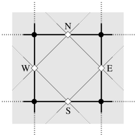
Figure 2.1. The four edges adjacent to a face on the square lattice.

Definition 1.

Let $\Omega$ be a square grid domain. Set $\lambda:=e^{\mathfrak{i}\pi/4}$. We say that $F\colon\Omega\to\mathbb{C}$ is s-holomorphic if for any face of $\Omega$ with edges $E,N,W,S$ (see Figure 2.1), the following s-holomorphicity equations hold

(2.1) $$F(N)+\lambda\overline{F(N)}=\; F(E)+\lambda\overline{F(E)}$$

$$F(N)+\lambda^{-1}\overline{F(N)}=\; F(W)+\lambda^{-1}\overline{F(W)}$$

$$F(S)+\lambda^{3}\overline{F(S)}=\; F(E)+\lambda^{3}\overline{F(E)}$$

$$F(S)+\lambda^{-3}\overline{F(S)}=\; F(W)+\lambda^{-3}\overline{F(W)}.$$

In other words $F\colon\Omega\rightarrow\mathbb{C}$ is s-holomorphic if for any pair of incident edges $e_{v}=\left\langle uv\right\rangle$ and $e_{w}=\left\langle uw\right\rangle$, we have $F\left(e_{v}\right)+\frac{\mathfrak{i}}{\theta}\overline{F\left(e_{v}\right)}=F\left(e_{w}\right)+\frac{\mathfrak{i}}{\theta}\overline{F\left(e_{w}\right)}$, where $\theta=\frac{2u-v-w}{\left|2u-v-w\right|}$. Equivalently, the orthogonal projections (in the complex plane) of $F\left(e_{v}\right)$ and $F\left(e_{w}\right)$ on the line $\sqrt{\frac{i}{\theta}}\mathbb{R}$ coincide.

The above equations imply (but are not equivalent to) the usual lattice Cauchy-Riemann equations: for the four edges around a face as in Figure 2.1 we have $F\left(N\right)-F\left(S\right)=\mathfrak{i}\left(F\left(E\right)-F\left(W\right)\right)$, and a similar equation holds for the four edges incident to a vertex. Discrete Cauchy-Riemann equations imply in turn the discrete Laplace equation $\sum_{Z=X\pm 1,X\pm i}\left(F\left(Z\right)-F\left(X\right)\right)=0$ for every edge $X\in\Omega\setminus\partial\Omega$.

2.2. Massive s-holomorphicity

We now define a perturbation of s-holomorphicity which we call massive s-holomorphicity. The massive s-holomorphicity equations with parameter $\beta$ are $\mathbb{R}$-linear equations satisfied by the Ising model parafermionic observables at inverse temperature $\beta$. At the critical point $\beta=\beta_{c}$, massive s-holomorphicity reduces to s-holomorphicity.

Definition 2.

Let $\beta>0$, let $\nu=\nu\left(\beta\right)$ be the unit complex number be defined by $\nu=\overline{\lambda}^{3}\frac{\alpha+i}{\alpha-i}$, where $\alpha=e^{-2\beta}$ and $\lambda=e^{\mathfrak{i}\pi/4}$. A function $F\colon\Omega\rightarrow\mathbb{C}$ is said to be massive s-holomorphic with parameter $\beta$ if for any face of $\Omega$ with edges $E,N,W,S$, we have

(2.2) $$F(N)+\nu^{-1}\lambda\overline{F(N)}=\; \nu^{-1}F(E)+\lambda\overline{F(E)}$$

$$F(N)+\nu\lambda^{-1}\overline{F(N)}=\; \nu F(W)+\lambda^{-1}\overline{F(W)}$$

$$F(S)+\nu\lambda^{3}\overline{F(S)}=\; \nu F(E)+\lambda^{3}\overline{F(E)}$$

$$F(S)+\nu^{-1}\lambda^{-3}\overline{F(S)}=\; \nu^{-1}F(W)+\lambda^{-3}\overline{F(W)}.$$

At $\beta=\beta_{c}$, we have $\nu=1$ and these equations coincide with the Equations (2.1) defining s-holomorphicity. It can be shown (see [BeDC10]) that massive s-holomorphicity implies (but is not equivalent to) the massive Laplace equation

$$\frac{1}{4}\sum_{Z=X\pm 1,X\pm i}\left(F\left(Z\right)-F\left(X\right)\right)=\mu F\left(X\right)\quad\forall X\in\Omega\setminus\partial\Omega,$$

with the mass $\mu=\mu(\beta)$ given by $\mu=\frac{S+S^{-1}}{2}-1$, where $S=\sinh\left(2\beta\right)$. The dual inverse temperatures $\beta$ and $\beta^{*}$, related by $\sinh(2\beta)\sinh(2\beta^{*})=1$, have equal masses $\mu(\beta)=\mu(\beta^{*})$, and at the critical point the mass vanishes $\mu(\beta_{c})=0$.

2.3. Riemann boundary values

The boundary conditions that are relevant for the study of Ising model specify the argument of a function on the boundary edges $\partial\Omega$: these conditions are trivially satisfied by the Ising parafermionic observables for topological reasons (see Section 4.3), at any temperature.

Let $\Omega$ be a discrete square grid domain. The boundary $\partial\Omega$ of $\Omega$ is a simple closed curve. For an edge $e\in\partial\Omega$, this defines a clockwise orientation $\tau_{\mathrm{cw}}\left(e\right)$ of $e$, which we view as a complex number: $\tau_{\mathrm{cw}}\left(e\right)\in\left\{\pm 1\right\}$ if $e$ is horizontal and $\tau_{\mathrm{cw}}\left(e\right)=\left\{\pm\mathfrak{i}\right\}$ if $e$ is vertical.

Definition 3.

We say that a function $f:\Omega\to\mathbb{C}$ satisfies Riemann boundary conditions $f\parallel\tau_{\mathrm{cw}}^{-\frac{1}{2}}$ at an edge $z\in\partial\Omega$ if

$$f\left(z\right)\parallel\tau_{\mathrm{cw}}^{-\frac{1}{2}}\left(z\right),$$

i.e. $f\left(z\right)$ is a real multiple of $\tau_{\mathrm{cw}}^{-\frac{1}{2}}\left(z\right)$.

When $\Omega$ is a rectangular box $\mathbf{I}\times\mathbf{J}$, the condition $f\parallel\tau_{\mathrm{cw}}^{-\frac{1}{2}}$ means that $f$ is purely real on the top side of $\Omega$, purely imaginary on the bottom side, a real multiple of $\lambda=e^{\mathfrak{i}\pi/4}$ on the left side and a real multiple of $\lambda^{-1}=e^{-\mathfrak{i}\pi/4}$ on the right side.

2.4. S-holomorphic continuation operator

For a (massive) s-holomorphic function on a rectangular box with Riemann boundary conditions $\parallel\tau_{\mathrm{cw}}^{-\frac{1}{2}}$, we can propagate its values row by row as illustrated in Figure 2.2. This is supplied by the following lemma (we use the same notation as in Section 1.3.1).

Lemma 4.

Consider the box $\mathbf{I}\times\left\{0,1\right\}$ for an integer interval $\mathbf{I}=\left[a,b\right]\cap\mathbb{Z}$ and let $\mathbf{I^{*}}=[a,b]\cap(\mathbb{Z}+\frac{1}{2})$ be its dual.

Let $f:\mathbf{I}_{0}^{*}\to\mathbb{C}$ be a complex-valued function and let $\beta>0$. Then there is a unique massive s-holomorphic extension $h$ of $f$ to $\mathbf{I}_{0}^{*}\cup\mathbf{I}_{\frac{1}{2}}\cup\mathbf{I}_{1}^{*}$ with Riemann boundary values on $\partial\mathbf{I}_{\frac{1}{2}}$.

Proof.

For $z\in\mathbf{I}_{\frac{1}{2}}\setminus\partial\mathbf{I}_{\frac{1}{2}}$, the value $h\left(z\right)$ can be solved uniquely from the last two of Equations (2.2) in terms of $f\left(z-\frac{1}{2}-\frac{i}{2}\right)$ and $f\left(z+\frac{1}{2}-\frac{i}{2}\right)$. For $z\in\partial\mathbf{I}_{\frac{1}{2}}$, the value $h\left(z\right)$ can be solved uniquely from the Riemann boundary condition and (2.2) in terms the value $f\left(z-\frac{i}{2}\pm\frac{1}{2}\right)$ ($\pm$ depending on whether $z$ is on the left or the right part of $\partial\mathbf{I}_{\frac{1}{2}}$). For $z\in\mathbf{I}_{1}^{{}^{*}}$, $h\left(z\right)$ can be solved in terms of $h$ at $z+\frac{1}{2}-\frac{i}{2}\in\mathbf{I}_{\frac{1}{2}}$ and $z-\frac{1}{2}-\frac{i}{2}\in\mathbf{I}_{\frac{1}{2}}$ by the first two of Equations (2.2). The definition of $h$ thus obtained satisfies all the required equations. ∎

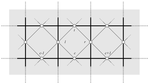
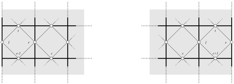
Figure 2.2. The values of a massive s-holomorphic function in the row above can be solved in terms of the values in the row below, both in the bulk and on the boundary.

Definition 5.

Let $\mathbf{I}$ be an interval of $\mathbb{Z}$ as above. We define the $\beta$-massive s-holomorphic propagator $P_{\beta}:\left(\mathbb{R}^{2}\right)^{\mathbf{I}^{*}}\to\left(\mathbb{R}^{2}\right)^{\mathbf{I}^{*}}$ by $P_{\beta}f=h\big{|}_{\mathbf{I}_{1}^{*}}$, where $f$ and $h$ are as in Lemma 4

We can explicitly write down the s-holomorphic propagator in critical and massive cases. The explicit form will be useful in the next section.

Lemma 6.

Let $\mathbf{I}^{*}=\left\{a+\frac{1}{2},a+\frac{3}{2},\ldots,b-\frac{1}{2}\right\}$ and denote the left and right extremities by $k_{L}=a+\frac{1}{2}$ and $k_{R}=b-\frac{1}{2}$. Set $\lambda:=e^{\mathfrak{i}\pi/4}$. The s-holomorphic propagator $P$ is given by

$$\begin{cases}\big{(}P\,f\big{)}(k)=&\frac{\lambda^{-3}}{\sqrt{2}}\,f(k-1)+2\,f(k)+\frac{\lambda^{3}}{\sqrt{2}}\,f(k+1)\\ &+\frac{1}{\sqrt{2}}\,\overline{f(k-1)}-\sqrt{2}\>\overline{f(k)}+\frac{1}{\sqrt{2}}\,\overline{f(k+1)}\qquad\qquad\forall k\in\mathbf{I}^{*}\setminus\left\{k_{L},k_{R}\right\}\\ \big{(}P\,f\big{)}(k_{L})=&\left(1+\frac{1}{\sqrt{2}}\right)f(k_{L})+\frac{\lambda^{3}}{\sqrt{2}}\,f(k_{L}+1)\\ &+\left(\lambda^{3}+\frac{\lambda^{-3}}{\sqrt{2}}\right)\overline{f(k_{L})}+\frac{1}{\sqrt{2}}\overline{f(k_{L}+1)}\\ \big{(}P\,f\big{)}(k_{R})=&\frac{\lambda^{-3}}{\sqrt{2}}\,f(k_{R}-1)+\left(1+\frac{1}{\sqrt{2}}\right)f(k_{R})\\ &+\frac{1}{\sqrt{2}}\overline{f(k_{R}-1)}+\left(\lambda^{-3}+\frac{\lambda^{3}}{\sqrt{2}}\right)\overline{f(k_{R})}.\end{cases}$$

For $\beta\neq\beta_{c}$, denote $S:=\sinh\left(2\beta\right)$, $C:=\cosh\left(2\beta\right)$. The massive s-holomorphic propagator $P_{\beta}$ is given by

$$\begin{cases}\big{(}P_{\beta}\,f\big{)}(k)=&\frac{-S-\mathfrak{i}}{2S}f(k-1)+\frac{C^{2}}{S}\,f(k)+\frac{-S+\mathfrak{i}}{2S}f(k+1)\\ &+\frac{C}{2S}\overline{f(k-1)}-C\overline{f(k)}+\frac{C}{2S}\overline{f(k+1)}\qquad\qquad\forall k\in\mathbf{I}^{*}\setminus\left\{k_{L},k_{R}\right\}\\ \big{(}P_{\beta}\,f\big{)}(k_{L})=&\frac{(S+C)C}{2S}\,f(k_{L})+\frac{-S+\mathfrak{i}}{2S}\,f(k_{L}+1)\\ &+\frac{-(S+C)S+\mathfrak{i}(C-S)}{2S}\,\overline{f(k_{L})}+\frac{C}{2S}\,\overline{f\left(k_{L}+1\right)}\\ \big{(}P_{\beta}\,f\big{)}(k_{R})=&\frac{-S-\mathfrak{i}}{2S}\,f(k_{R}-1)+\left(\frac{(S+C)C}{2S}\right)\,f(k_{R})\\ &+\frac{C}{2S}\,\overline{f(k_{R}-1)}+\left(\frac{-(S+C)S+\mathfrak{i}(C-S)}{2S}\right)\,\overline{f(k_{R})}.\end{cases}$$

2.5. Spectral splitting of the propagator

Proposition 7.

The matrix $P^{\beta}$ is symmetric, with eigenvalues $\lambda_{\alpha}^{\pm 1}$, where $\lambda_{\alpha}>1$ are distinct for $\alpha=1,\ldots,\left|\mathbf{I}\right|^{*}$.

Proof.

Clearly $P_{\beta}$ is invertible: the inverse of $P_{\beta}$ is the propagation of values of a massive s-holomorphic function downwards. Notice that exchanging $S$ and $N$ in the massive s-holomorphic equations (2.2) amounts to replacing $F$ by $\mathfrak{i}\overline{F}$. Denoting by $j:\left(\mathbb{R}^{2}\right)^{\mathbf{I}^{*}}\to\left(\mathbb{R}^{2}\right)^{\mathbf{I}^{*}}$ the (real-linear) involution $f\mapsto\mathfrak{i}\overline{f}$, we deduce that $\left(P_{\beta}\right)^{-1}=j\circ P_{\beta}\circ j^{-1}$. We deduce that the spectrum of $P_{\beta}$ is the same as the one of $\left(P_{\beta}\right)^{-1}$ and hence that the eigenvalues are of the form $\lambda_{\alpha}^{\pm 1}$ with $\lambda_{\alpha}\neq 0$ for $\alpha=1,\ldots,\left|\mathbf{I}^{*}\right|$.

For $\eta\in\mathbb{C}$, observe that the real-linear transpose of the map $z\mapsto\eta z$ is $z\mapsto\overline{\eta}z$ and that the map $z\mapsto\eta\overline{z}$ is real-symmetric. From the formula of Lemma 6, we deduce that $P_{\beta}$ is symmetric. To show that $P_{\beta}$ is positive definite, it is enough to show this at the critical temperature $\beta=\beta_{c}$, since the eigenvalues of $P_{\beta}$ are continuous in $\beta$ and cannot be zero. We can write the propagator $P_{\beta}$ as $BA$, where $A:\left(\mathbb{R}^{2}\right)^{\mathbf{I}^{*}}\to\left(\mathbb{R}^{2}\right)^{\mathbf{I}}$ is the propagation of $f:\mathbf{I}_{0}^{*}\to\mathbb{C}$ to $\mathbf{I}_{\frac{1}{2}}$ (see Definition 2) and $B:\left(\mathbb{R}^{2}\right)^{\mathbf{I}}\to\left(\mathbb{R}^{2}\right)^{\mathbf{I}^{*}}$ is the propagation of $g:\mathbf{I}_{\frac{1}{2}}\to\mathbb{C}$ to $\mathbf{I}_{1}^{*}$. At $\beta=\beta_{c}$, we have that $B=A^{\top}$ and hence $P=A^{\top}A$ is positive definite.

Let us now show that $1$ cannot be an eigenvalue. Suppose $f:\mathbf{I}_{0}^{*}\to\mathbb{C}$ is such that $P_{\beta}f=f$; we want to show that $f=0$. Let $h:\mathbf{I}_{0}^{*}\cup\mathbf{I}_{\frac{1}{2}}\cup\mathbf{I}_{1}^{*}\to\mathbb{C}$ denote the massive s-holomorphic extension of $f$.

At $\beta=\beta_{c}$ (i.e. when $P_{\beta}=P$), there is a particularly simple argument. Since $h$ satisfies the discrete Cauchy-Riemann equations, i.e. for any $x\in\mathbf{I}_{\frac{1}{2}}^{*}$, we have

$$h\left(x+\frac{1}{2}\right)-h\left(x-\frac{1}{2}\right)=\frac{1}{\mathfrak{i}}\left(h\left(x+\frac{\mathfrak{i}}{2}\right)-h\left(x-\frac{\mathfrak{i}}{2}\right)\right)=\frac{1}{\mathfrak{i}}\left(f\left(x\right)-f\left(x\right)\right)=0.$$

Hence $h$ must be constant on $\mathbf{I}_{\frac{1}{2}}$ and the Riemann boundary conditions easily imply that $h=0$. In turn, this implies that $f=0$, by the s-holomorphicity equations.

For general $\beta$, writing $\mathbf{I}_{\frac{1}{2}}=\left\{x_{L},x_{L}+1,\ldots,x_{R}\right\}$, we can deduce (from an explicit computation) that $h\left(x+1\right)$ and $h\left(x\right)$ (for $x\in\left\{x_{L},\ldots,x_{R}-1\right\}$) satisfy a linear relation:

(2.3) $$h\left(x+1\right)+\mathfrak{i}\mathcal{B}\overline{h\left(x+1\right)}=h\left(x\right)-\mathfrak{i}\mathcal{B}\overline{h\left(x\right)},$$

for $\mathcal{B}=\sqrt{2}\Im\mathfrak{m}\left(\nu\right)$, where $\nu=e^{\mathfrak{i}3\pi/4}\frac{\alpha+\mathfrak{i}}{\alpha-\mathfrak{i}}$ and $\alpha=e^{-2\beta}$ as above.

The Riemann boundary condition on the left extremity imposes that $h\left(x_{L}\right)=\mathcal{C}e^{-\mathfrak{i}\pi/4}$ for some $\mathcal{C}\in\mathbb{R}$, and the above equation (2.3) yields $h\left(x\right)=\mathcal{C}e^{-\mathfrak{i}\pi/4}\mathcal{A}^{x-x_{L}}$ where $\mathcal{A}=\frac{1+\mathcal{B}}{1-\mathcal{B}}\neq 0$. But the Riemann boundary condition on the right extremity, $h\left(x_{R}\right)\parallel e^{\mathfrak{i}\pi/4}$, then requires that $\mathcal{C}\mathcal{A}^{x_{R}-x_{L}}=0$ and hence $h=0$ everywhere by the massive s-holomorphic equations.

Finally we show that the eigenvalues are distinct. Suppose $\Lambda>0$ is an eigenvalue of $P_{\beta}$, and let $f_{\Lambda}\in(\mathbb{R}^{2}){}^{\mathbf{I}^{*}}$ is an eigenvector, and let $h_{\Lambda}$ be the massive s-holomorphic extension of $f_{\Lambda}$ to $\mathbf{I}_{0}^{*}\cup\mathbf{I}_{\frac{1}{2}}\cup\mathbf{I}_{1}^{*}$. The massive s-holomorphicity equations can be solved to obtain a recursion relation $h_{\Lambda}(x+1)=\eta h_{\Lambda}(x)+\eta^{\prime}\overline{h_{\Lambda}(x)}$ with some explicit $\eta,\eta^{\prime}\in\mathbb{C}$. This shows that the eigenspace is one-dimensional. ∎

3. Transfer Matrix, Clifford Algebra and Induced Rotation

In this section we review fundamental algebraic structures underlying the transfer matrix formalism introduced in [Kau49]. See [Pal07] for a recent exposition with more details.

3.1. Transfer matrix and Clifford algebra

In the introduction, Section 1.2.1, we defined the Ising transfer matrix $V:\mathcal{S}\to\mathcal{S}$ with fixed boundary conditions at the two extremities of the row $\mathbf{I}=\left\{a,a+1,\ldots,b-1,b\right\}$ as the product

$$V=\; (V^{\mathrm{h}})^{\frac{1}{2}}\,V^{\mathrm{v}}\,(V^{\mathrm{h}})^{\frac{1}{2}},$$

where the matrix elements in the basis $(\mathbf{e}_{\sigma})$ indexed by spin configurations in a row, $\sigma\in\left\{\pm 1\right\}^{\mathbf{I}}$, are given by

$$V_{\sigma\rho}^{\mathrm{v}}=\begin{cases}\exp\left(\beta\sum_{i=a}^{b}\sigma_{i}\rho_{i}\right)\quad&\mbox{if }\sigma_{a}=\rho_{a}\text{ and }\sigma_{b}=\rho_{b}\\ 0\qquad&\mbox{otherwise}\end{cases}$$

and

$$\left(V_{\sigma\rho}^{\mathrm{h}}\right)^{\frac{1}{2}}=\begin{cases}\exp\left(\frac{\beta}{2}\sum_{i=a}^{b-1}\sigma_{i}\sigma_{i+1}\right)\quad&\mbox{if }\sigma\equiv\rho\\ 0\qquad&\mbox{otherwise}.\end{cases}$$

There is a two-fold degeneracy in the spectrum of the transfer matrix: the global spin flip $\sigma\mapsto-\sigma$ commutes with both $V^{\mathrm{v}}$ and $\left(V^{\mathrm{h}}\right)^{\frac{1}{2}}$. To disregard the corresponding multiplicity of eigenvalues, we restrict our attention to the subspace

$$\mathcal{S}_{+}=\; \mathrm{span}\left\{\mathbf{e}_{\sigma}\,\big{|}\,\sigma_{b}=+1\right\},$$

spanned by spin configurations that have a plus spin on the right extremity of the row. This subspace is invariant for both $V^{\mathrm{v}}$ and $\left(V^{\mathrm{h}}\right)^{\frac{1}{2}}$. Note that the dimension is given by

$$\mathrm{dim}\left(\mathcal{S}_{+}\right)=\; 2^{|\mathbf{I}|-1}=2^{|\mathbf{I}^{*}|}=2^{b-a}.$$

In Section 1.3.2, we defined also the operators $p_{k}$ and $q_{k}$ on $\mathcal{S}$, for $k\in\mathbf{I}^{*}=\left\{a+\frac{1}{2},\,a+\frac{3}{2},\,\ldots,\,b-\frac{3}{2},\,b-\frac{1}{2}\right\}$, by

$$\begin{array}[]{c}p_{k}\left(\mathbf{e}_{\sigma}\right)=\;\sigma_{k+\frac{1}{2}}\mathbf{e}_{\tau}\\ q_{k}\left(\mathbf{e}_{\sigma}\right)=\mathfrak{i}\,\sigma_{k-\frac{1}{2}}\mathbf{e}_{\tau}\end{array}\qquad\text{, where} \tau_{x}=\; \begin{cases}\phantom{-}\sigma_{x\quad}&\text{for }x>k\\ -\sigma_{x}\quad&\text{for }x<k.\end{cases}$$

Again, the subspace $\mathcal{S}_{+}\subset\mathcal{S}$ is invariant for all $p_{k},q_{k}$. We denote $\mathcal{W}=\mathrm{span}\left\{p_{k},q_{k}\,\big{|}\,k\in\mathbf{I}^{*}\right\}\subset{\rm End}(\mathcal{S})$.

It is easy to check that $p_{k},q_{k}$ satisfy the relations

$$p_{k}p_{\ell}+p_{\ell}p_{k} = 2\,\delta_{k,\ell}\,\mathrm{id}_{\mathcal{S}}$$

$$q_{k}q_{\ell}+q_{\ell}q_{k} = 2\,\delta_{k,\ell}\,\mathrm{id}_{\mathcal{S}}$$

$$p_{k}q_{\ell}+q_{\ell}p_{k} = 0,$$

i.e. that they form a Clifford algebra representation on $\mathcal{S}_{+}$ and on $\mathcal{S}$. This representation is faithful, so we think of the Clifford algebra $\mathfrak{Cliff}$ simply as the algebra of linear operators $\mathcal{S}\rightarrow\mathcal{S}$ generated by $\mathcal{W}$.

Consider the symmetric bilinear form $(\cdot,\cdot)$ on $\mathcal{W}$ given by $(p_{k},p_{l})=2\delta_{k,l}$, $(q_{k},q_{l})=2\delta_{k,l}$, $(p_{k},q_{l})=0$. Then $\mathfrak{Cliff}$ is the algebra with set of generators $\mathcal{W}$ and relations $uv+vu=(u,v)\,\mathbf{1}$, for $u,v\in\mathcal{W}$. The dimensions of the set of Clifford generators and the Clifford algebra are

$$\mathrm{dim}(\mathcal{W})=\; 2|\mathbf{I}^{*}|=2(b-a), \mathrm{dim}(\mathfrak{Cliff})=\; 2^{\mathrm{dim}(\mathcal{W})}=2^{2|\mathbf{I}^{*}|}=2^{2(b-a)}.$$

The transfer matrix can be written in terms of exponentials of quadratic expressions in the Clifford algebra generators as follows.

Proposition 8.

We have

$$\left(V^{\mathrm{h}}\right)^{\frac{1}{2}} = \exp\left(\mathfrak{i}\frac{\beta}{2}\sum_{k\in\mathbf{I}^{*}}q_{k}p_{k}\right)$$

$$V^{\mathrm{v}} = e^{2\beta}\left(2S\right)^{\frac{\left|\mathbf{I}\right|}{2}-1}\;\exp\left(\mathfrak{i}\beta^{*}\sum_{j\in\mathbf{I}\setminus\partial\mathbf{I}}p_{j-\frac{1}{2}}q_{j+\frac{1}{2}}\right),$$

where $\beta^{*}$ is the dual inverse temperature given by $\tanh\left(\beta^{*}\right)=e^{-2\beta}$ and $S=\sinh\left(2\beta\right)$.

Proof.

Note that the operator $\mathfrak{i}\,q_{k}p_{k}$ has the following diagonal action in the basis $(\mathbf{e}_{\sigma})$

$$\mathfrak{i}\,q_{k}p_{k}\;\mathbf{e}_{\sigma}=\; \sigma_{k+\frac{1}{2}}\sigma_{k-\frac{1}{2}}\;\mathbf{e}_{\sigma},$$

so the first asserted result $e^{\mathfrak{i}\frac{\beta}{2}\sum_{k}q_{k}p_{k}}=(V^{\mathrm{h}})^{\frac{1}{2}}$ follows immediately. The operator $\mathfrak{i}\,p_{j-\frac{1}{2}}q_{j+\frac{1}{2}}$ inverts the value of the spin at $j$,

$$\mathfrak{i}\,p_{j-\frac{1}{2}}q_{j+\frac{1}{2}}\;\mathbf{e}_{\sigma}=\; \mathbf{e}_{\sigma^{\prime}},\qquad\text{where }\sigma_{x}^{\prime}=\begin{cases}\phantom{-}\sigma_{x}\qquad&\text{for }x\neq j\\ -\sigma_{j}\qquad&\text{for }x=j,\end{cases}$$

so we have

$$\exp\left(\mathfrak{i}\beta^{*}p_{j-\frac{1}{2}}q_{j+\frac{1}{2}}\right)\,\mathbf{e}_{\sigma}=\; \cosh(\beta^{*})\,\mathbf{e}_{\sigma}+\sinh(\beta^{*})\,\mathbf{e}_{\sigma^{\prime}}.$$

Taking $\beta^{*}$ such that $\tanh\left(\beta^{*}\right)=e^{-2\beta}$ and computing the product of these commuting operators at different $j$ we get

$$\exp\left(\mathfrak{i}\beta^{*}\sum_{j=a+1}^{b-1}p_{j-\frac{1}{2}}q_{j+\frac{1}{2}}\right)\,\mathbf{e}_{\sigma}=\; \cosh(\beta^{*})^{b-a-1}\sum_{\begin{subarray}{c}\rho\in\left\{\pm 1\right\}^{\mathbf{I}}\\ \rho_{a}=\sigma_{a},\;\rho_{b}=\sigma_{b}\end{subarray}}\tanh(\beta^{*})^{\#\{x|\sigma_{x}\neq\rho_{x}\}}\,\mathbf{e}_{\rho}$$

$$=\; e^{-2\beta}\left(2S\right)^{1-\frac{\left|\mathbf{I}\right|}{2}}\sum_{\begin{subarray}{c}\rho\in\left\{\pm 1\right\}^{\mathbf{I}}\\ \rho_{a}=\sigma_{a},\;\rho_{b}=\sigma_{b}\end{subarray}}\exp\left(\sum_{i=a+1}^{b-1}\sigma_{i}\rho_{i}\right)\,\mathbf{e}_{\rho},$$

which is the second asserted result. ∎

3.2. Induced rotation

Since the constituents of the transfer matrix are exponentials of second order polynomials in the Clifford generators, conjugation by the transfer matrix stabilizes the set of Clifford generators. In the formulas below, we use the notation

$$s=\; \sinh(\beta)\qquad s^{*}=\; \sinh(\beta^{*})$$

$$c=\; \cosh(\beta)\qquad c^{*}=\; \cosh(\beta^{*})$$

$$S=\; \sinh(2\beta)=\frac{1}{\sinh(2\beta^{*})}\qquad C=\; \cosh(2\beta)=\frac{\cosh(2\beta^{*})}{\sinh(2\beta^{*})}.$$

The following lemma is a result of straightforward calculations, which can be found e.g. in [Pal07].

Lemma.

Conjugation by $V^{\mathrm{h}}$ is given by the following formulas on Clifford generators $p_{k},q_{k}$ ($k\in\mathbf{I}^{*}$)

$$\left(V^{\mathrm{h}}\right)^{-\frac{1}{2}}\circ p_{k}\circ\left(V^{\mathrm{h}}\right)^{\frac{1}{2}}=\; c\,p_{k}-\mathfrak{i}s\,q_{k}$$

$$\left(V^{\mathrm{h}}\right)^{-\frac{1}{2}}\circ q_{k}\circ\left(V^{\mathrm{h}}\right)^{\frac{1}{2}}=\; \mathfrak{i}s\,p_{k}+c\,q_{k}.$$

Let $k_{L}=a+\frac{1}{2}$ and $k_{R}=b-\frac{1}{2}$ be the leftmost and rightmost points of $\mathbf{I}^{*}$. Conjugation by $V^{\mathrm{v}}$ is given by

$$\left(V^{{\rm v}}\right)^{-1}\circ p_{k}\circ V^{{\rm v}}=\; \frac{C}{S}\,p_{k}+\frac{\mathfrak{i}}{S}\,q_{k+1}\qquad\text{for }k\neq k_{R}$$

$$\left(V^{{\rm v}}\right)^{-1}\circ q_{k}\circ V^{{\rm v}}=\; \frac{-\mathfrak{i}}{S}\,p_{k-1}+\frac{C}{S}\,q_{k}\qquad\text{for }k\neq k_{L}$$

and on the remaining generators by

$$\left(V^{{\rm v}}\right)^{-1}\circ p_{k_{R}}\circ V^{{\rm v}}=\; p_{k_{R}}\qquad \left(V^{{\rm v}}\right)^{-1}\circ q_{k_{L}}\circ V^{{\rm v}}=\; q_{k_{L}}.$$

We see that $\mathcal{W}\subset\mathrm{End}(\mathcal{S})$ is an invariant subspace for the conjugation by the transfer matrix $V$. The conjugation is called the induced rotation of $V$, and denoted by

$$T_{V}\colon\; \mathcal{W}\rightarrow\mathcal{W}\qquad T_{V}(w)=\; V\circ w\circ V^{-1}.$$

Note that the induced rotation $T_{V}$ preserves the bilinear form, $(T_{V}u,\,T_{V}v)=(u,v)$ for all $u,v\in\mathcal{W}$.

We will next show that the induced rotation is, up to a change of basis, the complexification of the row-to-row propagation $P_{\beta}$ of massive s-holomorphic functions satisfying the Riemann boundary condition. To facilitate the calculations, we introduce two symmetry operations on the set of Clifford algebra generators. We define a (complex) linear isomorphism $R\colon\mathcal{W}\rightarrow\mathcal{W}$ and a (complex) conjugate-linear isomorphism $J\colon\mathcal{W}\rightarrow\mathcal{W}$ by the formulas

$$R(p_{k})=\; \mathfrak{i}\,q_{a+b-k}\quad R(q_{k})=\; -\mathfrak{i}\,p_{a+b-k}\quad$$ (extended linearly)

$$J(p_{k})=\; \mathfrak{i}\,p_{k}\quad J(q_{k})=\; -\mathfrak{i}\,q_{k}\quad \text{(extended conjugate-linearly)}.$$

We will moreover use for $\mathcal{W}$ the basis

$$\psi_{k}=\; \frac{\mathfrak{i}}{\sqrt{2}}(p_{k}+q_{k}), \bar{\psi}_{k}=\; \frac{1}{\sqrt{2}}(p_{k}-q_{k}), k\in\mathbf{I}^{*}.$$

Lemma 9.

The maps $R$ and $J$ commute with $T_{V}$, i.e. we have

$$T_{V}\circ R=\; R\circ T_{V}, T_{V}\circ J=\; J\circ T_{V}.$$

For all $k\in\mathbf{I}^{*}$ we have

$$R(\psi_{k})=\; \bar{\psi}_{b+a-k}, R(\bar{\psi}_{k})=\; \psi_{b+a-k}$$

$$J(\psi_{k})=\; \bar{\psi}_{k}, J(\bar{\psi}_{k})=\; \psi_{k}.$$

Proof.

By the explicit expressions of Lemma Lemma one easily verifies that $R$ and $J$ commute with the conjugation by both $\left(V^{{\rm h}}\right)^{\frac{1}{2}}$ and $V^{{\rm v}}$.∎

Theorem 10.

The induced rotation $T_{V}\colon\mathcal{W}\rightarrow\mathcal{W}$ is up to a change of basis equal to the complexification of $P_{\beta}$, i.e. there exists a linear isomorphism $\varrho:\left(\mathbb{C}^{2}\right)^{\mathbf{I}^{*}}\to\mathcal{W}$ such that $T_{V}=\varrho\circ P^{\mathbb{C}}\circ\varrho^{-1}$.

Proof.

Consider the action of the induced rotation in the basis $(\psi_{k},\bar{\psi}_{k})_{k\in\mathbf{I}^{*}}$. With the formulas of Lemma Lemma, it is straighforward to compute that for $k\in\mathbf{I}^{*}\setminus(\partial\mathbf{I}^{*})$

$$T_{V}^{-1}(\psi_{k})=\; \frac{C^{2}}{S}\,\psi_{k}+\left(-\frac{1}{2}-\frac{\mathfrak{i}}{2S}\right)\,\psi_{k-1}+\left(-\frac{1}{2}+\frac{\mathfrak{i}}{2S}\right)\,\psi_{k+1}$$

$$-C\,\bar{\psi}_{k}+\frac{1}{2}\frac{C}{S}\,\bar{\psi}_{k-1}+\frac{1}{2}\frac{C}{S}\,\bar{\psi}_{k+1}.$$

To get a formula for $T_{V}^{-1}(\bar{\psi}_{k})$, $k\in\mathbf{I}^{*}\setminus(\partial\mathbf{I}^{*})$, apply the map $J$ on this and use Lemma 9. We still need formulas for the two extremities, $k\in\partial\mathbf{I}^{*}=\left\{a+\frac{1}{2},b-\frac{1}{2}\right\}$. On the left extremity, at $k_{L}=a+\frac{1}{2}$, a straightforward calculation yields

$$T_{V}^{-1}(\psi_{k_{L}})=\; \frac{C(S+C)}{2S}\,\psi_{k_{L}}+\frac{(1+\mathfrak{i}S)}{2S}\mathfrak{i}\,\psi_{k_{L}+1}$$

$$+\frac{-S(C+S)+\mathfrak{i}(C-S)}{2S}\,\bar{\psi}_{k_{L}}+\frac{C}{2S}\,\bar{\psi}_{k_{L}+1}.$$

To get a formula for $T_{V}^{-1}(\bar{\psi}_{k_{L}})$, apply the map $J$ on this. To get the formula for $T_{V}^{-1}(\bar{\psi}_{k_{R}})$, where $k_{R}=b-\frac{1}{2}$, apply the map $R$. To get a formula for $T_{V}^{-1}(\psi_{k_{R}})$, apply the composition $J\circ R$.

Since the coefficients in the formulas for $T_{V}^{-1}(\psi_{k})$ coincide with the coefficients in the formulas for $(P_{\beta}f)(k)$ in Section 2.4, and the coefficients in the formulas for $T_{V}^{-1}(\bar{\psi}_{k})$ are the complex conjugates of the corresponding ones, we get that the complexification of $P_{\beta}$ agrees with $T_{V}^{-1}$ up to a change of basis. This finishes the proof, because $P_{\beta}$ and its inverse $P_{\beta}^{-1}$ are conjugates by Proposition 7. ∎

3.3. Fock representations

Finite dimensional irreducible representations of the Clifford algebra $\mathfrak{Cliff}$ are Fock representations, defined below. To define a Fock representation, one first chooses a way to split the set $\mathcal{W}$ of Clifford algebra generators to creation and annihilation operators. Let $(\cdot,\cdot)$ denote the bilinear form on $\mathcal{W}$ defined in Section 3.1. A polarization (an isotropic splitting) is a choice of two complementary subspaces $\mathcal{W}_{\boxplus}$ (creation operators) and $\mathcal{W}_{\boxminus}$ (annihilation operators) of the set of Clifford algebra generators,

$$\mathcal{W}=\; \mathcal{W}_{\boxplus}\oplus\mathcal{W}_{\boxminus},$$

such that

$$(w_{\boxplus},w_{\boxplus}^{\prime})=\; 0\qquad\text{for all }w_{\boxplus},w_{\boxplus}^{\prime}\in\mathcal{W}_{\boxplus}$$

$$(w_{\boxminus},w_{\boxminus}^{\prime})=\; 0\qquad\text{for all }w_{\boxminus},w_{\boxminus}^{\prime}\in\mathcal{W}_{\boxminus}.$$

Note that due to the nondegeneracy of the bilinear form $(\cdot,\cdot)$, the two subspaces $\mathcal{W}_{\boxplus}$ and $\mathcal{W}_{\boxminus}$ are naturally dual to each other, and in particular

$$\mathrm{dim}(\mathcal{W}_{\boxplus})=\; \mathrm{dim}(\mathcal{W}_{\boxminus})=\frac{1}{2}\mathrm{dim}(\mathcal{W})=|\mathbf{I}^{*}|=b-a$$

is the number of linearly independent creation operators.

As a vector space, the Fock representation corresponding to the polarization $\mathcal{W}=\mathcal{W}_{\boxplus}\oplus\mathcal{W}_{\boxminus}$ is the exterior algebra of $\mathcal{W}_{\boxplus}$,

$$\bigwedge\mathcal{W}_{\boxplus}=\; \bigoplus_{n=0}^{|\mathbf{I}^{*}|}\left(\wedge^{n}\mathcal{W}_{\boxplus}\right).$$

To define the representation of the Clifford algebra on this vector space, let $(a_{\alpha}^{\dagger})_{\alpha=1}^{|\mathbf{I}^{*}|}$ be a basis of $\mathcal{W}_{\boxplus}$ and $(a_{\alpha})_{\alpha=1}^{|\mathbf{I}^{*}|}$ the dual basis of $\mathcal{W}_{\boxminus}$, i.e. $(a_{\alpha}^{\dagger},a_{\beta})=\delta_{\alpha,\beta}$. The action of the Clifford algebra on the Fock space $\bigwedge\mathcal{W}_{\boxplus}$ is given by the linear extension of the formulas

$$a_{\alpha}^{\dagger}.(a_{\beta_{1}}^{\dagger}\wedge a_{\beta_{2}}^{\dagger}\wedge\cdots\wedge a_{\beta_{n}}^{\dagger})=\; a_{\alpha}^{\dagger}\wedge a_{\beta_{1}}^{\dagger}\wedge a_{\beta_{2}}^{\dagger}\wedge\cdots\wedge a_{\beta_{n}}^{\dagger}$$

$$a_{\alpha}.(a_{\beta_{1}}^{\dagger}\wedge a_{\beta_{2}}^{\dagger}\wedge\cdots\wedge a_{\beta_{n}}^{\dagger})=\; \sum_{j=1}^{n}(-1)^{j-1}\delta_{\alpha,\beta_{j}}\;a_{\beta_{1}}^{\dagger}\wedge\cdots\wedge a_{\beta_{j-1}}^{\dagger}\wedge a_{\beta_{j+1}}^{\dagger}\wedge\cdots\wedge a_{\beta_{n}}^{\dagger}.$$

The vector $1\in\mathbb{C}\cong\wedge^{0}\mathcal{W}_{\boxplus}\subset\bigwedge\mathcal{W}_{\boxplus}$ is called the vacuum of the Fock representation: it is annihilated by all of $\mathcal{W}_{\boxminus}$. Irreducible representations are characterized by such vacuum vectors as follows.

Lemma 11.

Suppose that $\mathcal{W}=\mathcal{W}_{\boxplus}\oplus\mathcal{W}_{\boxminus}$ is a polarization. Any irreducible representation of $\mathfrak{Cliff}$ is isomorphic to the Fock representation $\bigwedge\mathcal{W}_{\boxplus}$. If a representation $\mathcal{V}$ of $\mathfrak{Cliff}$ contains a non-zero vector $v_{\mathrm{vac}}\in\mathcal{V}$ satisfying $\mathcal{W}_{\boxminus}v_{\mathrm{vac}}=0$, then the Fock space $\bigwedge\mathcal{W}_{\boxplus}$ embeds in $\mathcal{V}$ by the mapping

$$a_{\beta_{1}}^{\dagger}\wedge a_{\beta_{2}}^{\dagger}\wedge\cdots\wedge a_{\beta_{n}}^{\dagger}\mapsto\; (a_{\beta_{1}}^{\dagger}a_{\beta_{2}}^{\dagger}\cdots a_{\beta_{n}}^{\dagger}).v_{\mathrm{vac}}.$$

Proof.

Consider a representation $\mathcal{V}$ of $\mathfrak{Cliff}$. Choose a non-zero $v^{(0)}\in\mathcal{V}$. Define recursively $v^{(\alpha)}$, for $\alpha=1,2,\ldots|\mathbf{I}^{*}|$, to be $a_{\alpha}v^{(\alpha-1)}$ if this is non-vanishing and $v^{(\alpha-1)}$ otherwise. Then $v_{\mathrm{vac}}=v^{(|\mathbf{I}^{*}|)}$ is non-zero and $\mathcal{W}_{\boxminus}v_{\mathrm{vac}}=0$, i.e. $v_{\mathrm{vac}}$ is a vacuum vector. This argument shows in particular that any non-zero subrepresentation of the Fock representation $\bigwedge\mathcal{W}_{\boxplus}$ contains the vacuum vector $1\in\wedge^{0}\mathcal{W}_{\boxplus}$, and thus the Fock representation is irreducible. The mapping $\bigwedge\mathcal{W}_{\boxplus}\rightarrow\mathcal{V}$ given in the statement defines a non-zero intertwining map of Clifford algebra representations, and by irreducibility of the Fock representation, this is an embedding. If $\mathcal{V}$ is irreducible the embedding must be surjective, and thus an isomorphism. ∎

The fact that the Fock representation is the only isomorphism type of irreducible representations of the Clifford algebra would follow already from the irreducibility of the Fock representation and the observation that $\left(\mathrm{dim}(\bigwedge\mathcal{W}_{\boxplus})\right)^{2}=\mathrm{dim}(\mathfrak{Cliff})$, by the (Artin–)Wedderburn structure theorem.

A standard tool for performing calculations in the Fock representation is the following. We recall that the Pfaffian ${\rm Pf}(A)$ of an antisymmetric matrix $A\in\mathbb{C}^{n\times n}$ is zero if $n$ is odd, and if $n=2m$ is even, then it is given by

$${\rm Pf}(A)=\; \frac{1}{2^{m}\,m!}\sum_{\pi\in S_{2m}}\mathrm{sgn}(\pi)\,\prod_{s=1}^{m}A_{\pi(2s-1),\pi(2s)}.$$

Lemma 12 (Fermionic Wick’s formula).

Let $\mathcal{W}=\mathcal{W}_{\boxplus}\oplus\mathcal{W}_{\boxminus}$ be a polarization, and consider the Fock representation $\bigwedge\mathcal{W}_{\boxplus}$. Let $v_{{\rm vac}}=1\in\wedge^{0}\mathcal{W}_{\boxplus}\subset\bigwedge\mathcal{W}_{\boxplus}$ be the vacuum and $v_{{\rm vac}}^{*}\in\left(\wedge^{0}\mathcal{W}_{\boxplus}\right)^{*}\subset\left(\bigwedge\mathcal{W}_{\boxplus}\right)^{*}$ be the dual vacuum normalized by $\langle v_{{\rm vac}}^{*},v_{{\rm vac}}\rangle=1$. Then for any $\phi_{1},\ldots,\phi_{n}\in\mathcal{W}$ we have

$$\langle v_{{\rm vac}}^{*},\;\phi_{1}\cdots\phi_{n}v_{{\rm vac}}\rangle=\; \mathrm{Pf}\left(\Big{[}\langle v_{{\rm vac}}^{*},\,\phi_{i}\phi_{j}v_{{\rm vac}}\rangle\Big{]}_{i,j=1}^{n}\right).$$

Proof.

Write the elements $\phi_{i}\in\mathcal{W}$ as sums of creation and annihilation operators, and then anticommute the annihilation operators to the right and the creation operators to the left. ∎

3.4. A simple polarization for low temperature expansions

The following lemma gives one of the simplest possible polarizations.

Lemma 13.

The following formulas define a polarization

$$\mathcal{W}_{\boxplus}^{(+)}=\; \mathrm{span}\left\{p_{k}-\mathfrak{i}q_{k}\;\big{|}\;k\in\mathbf{I}^{*}\right\}$$

$$\mathcal{W}_{\boxminus}^{(+)}=\; \mathrm{span}\left\{p_{k}+\mathfrak{i}q_{k}\;\big{|}\;k\in\mathbf{I}^{*}\right\}.$$

Proof.

The vectors $p_{k}+\mathfrak{i}q_{k}$, $p_{k}-\mathfrak{i}q_{k}$ for $k\in\mathbf{I}^{*}$ form a basis of $\mathcal{W}$, and we have $(p_{k}\pm\mathfrak{i}q_{k},\,p_{l}\pm\mathfrak{i}q_{l})=2\delta_{k,l}+0+0+(\pm\mathfrak{i})^{2}\,2\delta_{k,l}=0$. ∎

Recall that in the state space $\mathcal{S}$ of the transfer matrix formalism we have the vectors corresponding to the constant spin configurations in a row,

$$\mathbf{e}_{(+)}\in\; \mathcal{S}_{+} (+)=\; (+1,+1,\ldots,+1)\in\left\{\pm 1\right\}^{\mathbf{I}}$$

$$\mathbf{e}_{(-)}\in\; \mathcal{S} (-)=\; (-1,-1,\ldots,-1)\in\left\{\pm 1\right\}^{\mathbf{I}}.$$

Directly from the defining formulas of the operators $p_{k},q_{k}$, one sees that the vectors $\mathbf{e}_{(+)},\mathbf{e}_{(-)}\in\mathcal{S}$ satisfy $(p_{k}+\mathfrak{i}q_{k})\mathbf{e}_{(+)}=0$ and $(p_{k}+\mathfrak{i}q_{k})\mathbf{e}_{(-)}=0$ for all $k\in\mathbf{I}^{*}$.

Corollary 14.

As a representation of the Clifford algebra, $\mathcal{S}_{+}$ is isomorphic to the Fock space $\bigwedge\mathcal{W}_{\boxplus}^{(+)}$, with vacuum vector $v_{{\rm vac}}^{(+)}=\mathbf{e}_{(+)}$, and $\mathcal{S}$ is isomorphic to the direct sum of two copies of this Fock space.

We emphasize that the polarization of this subsection is not the physical one, but by Lemma 11, the isomorphism type of the Fock representation doesn’t depend on the polarization, so the state space of the transfer matrix formalism is in fact a Fock representation for any polarization. The polarization is, however, the zero temperature limit ($\beta\nearrow\infty$) of the physical polarizations of the next section, and it is very closely related to the low temperature graphical expansions of correlation functions and observables considered in Sections 4.3, 4.4 and 4.5. In particular, a slight modification of this simple polarization together with the fermionic Wick’s formula will be used for the proof of Pfaffian formulas for fermion operator multi-point correlation functions and multi-point parafermionic observables. The modified polarization is the following.

Lemma 15.

Let $N\in\mathbb{N}$. The following formulas define a polarization

$$\mathcal{W}_{\boxplus}^{(+);N}=\; \mathrm{span}\left\{V^{-N}(p_{k}-\mathfrak{i}q_{k})V^{N}\;\big{|}\;k\in\mathbf{I}^{*}\right\}$$

$$\mathcal{W}_{\boxminus}^{(+)}=\; \mathrm{span}\left\{p_{k}+\mathfrak{i}q_{k}\;\big{|}\;k\in\mathbf{I}^{*}\right\}$$

for all $\beta$ except possibly for isolated values. The space $\mathcal{S}_{+}$ is isomorphic to a Fock representation $\bigwedge\left(\mathcal{W}_{\boxplus}^{(+);N}\right)$, with vacuum vector $v_{{\rm vac}}^{(+);N}=\mathbf{e}_{(+)}\in\mathcal{S}_{+}$ and dual vacuum vector $(v_{{\rm vac}}^{(+);N})^{*}=\frac{1}{\mathbf{e}_{(+)}^{\top}V^{N}\mathbf{e}_{(+)}}\times\mathbf{e}_{(+)}^{\top}V^{N}$.

Proof.

The special case $N=0$ was treated above. Since we have $(p_{k}\pm\mathfrak{i}q_{k},\,p_{l}\pm\mathfrak{i}q_{l})=0$ and the bilinear form is invariant under $T_{V}$, $(T_{V}^{-N}u,\,T_{V}^{-N}v)=(u,v)$, it follows that also for general $N$ the choice of subspaces is a polarization if the two subspaces span the whole space $\mathcal{W}$, that is if the vectors $T_{V}^{-N}(p_{k}-\mathfrak{i}q_{k})$ and $p_{k}+\mathfrak{i}q_{k}$ for $k\in\mathbf{I}^{*}$ form a basis of $\mathcal{W}$. It suffices to show that the matrix $\left[(p_{k}+\mathfrak{i}q_{k},\;T_{V}^{-N}(p_{l}-\mathfrak{i}q_{l}))\right]_{k,l\in\mathbf{I}^{*}}$ of the bilinear form is non-degenerate. The non-degeneracy is evident in the limit $\beta\nearrow\infty$, since $e^{-2\beta}T_{V}^{-1}(p_{k}-\mathfrak{i}q_{k})=p_{k}-\mathfrak{i}q_{k}+O(e^{-\beta})$ and $e^{-2\beta}T_{V}^{-1}(p_{k}+\mathfrak{i}q_{k})=O(e^{-\beta})$ by the formulas of Lemma Lemma. The determinant $\det\left(\left[(p_{k}+\mathfrak{i}q_{k},\;T_{V}^{-N}(p_{l}-\mathfrak{i}q_{l}))\right]_{k,l\in\mathbf{I}^{*}}\right)$ is analytic in $\beta$, so its (possible) zeroes can’t have accumulation points. We conclude that $\mathcal{W}=\mathcal{W}_{\boxplus}^{(+);N}\oplus\mathcal{W}_{\boxminus}^{(+)}$ is a polarization except possibly for isolated values of $\beta$.

The same calcuation as before shows that $\mathbf{e}_{(+)}$ is a vacuum vector of the Fock representation $\mathcal{S}_{+}\cong\bigwedge W_{\boxplus}^{(+);N}$, and similarly from the calculation $\mathbf{e}_{(+)}^{\top}(p_{k}-\mathfrak{i}q_{k})=0$ we get that the dual vacuum of $\mathcal{S}_{+}\cong\bigwedge W_{\boxplus}^{(+);N}$ is proportional to $\mathbf{e}_{(+)}^{\top}V^{N}$. ∎

3.5. The physical polarization

The relevant polarization and basis is the one in which the particle-states $a_{\beta_{1}}^{\dagger}a_{\beta_{2}}^{\dagger}\cdots a_{\beta_{n}}^{\dagger}.v_{{\rm vac}}$ are eigenvectors of the evolution defined by the transfer matrix. We make use of the fact that $1$ is not an eigenvalue of $T_{V}$, which follows from Proposition 7 and Theorem 10.

Lemma 16.

Let $\mathcal{W}_{\boxplus}^{{\rm phys}}\subset\mathcal{W}$ be the subspace spanned by eigenvectors of $T_{V}$ with eigenvalues less than one and $\mathcal{W}_{\boxminus}^{{\rm phys}}\subset\mathcal{W}$ the subspace spanned by eigenvectors of $T_{V}$ with eigenvalues greater than one. Then $\mathcal{W}_{\boxplus}^{{\rm phys}}\oplus\mathcal{W}_{\boxminus}^{{\rm phys}}$ is a polarization. As a representation of $\mathfrak{Cliff}$, the space $\mathcal{S}_{+}$ is isomorphic to the Fock representation $\bigwedge\mathcal{W}_{\boxplus}^{{\rm phys}}$.

Proof.

Recall that for any $u,v\in\mathcal{W}$ we have $(T_{V}u,T_{V}v)=(u,v)$. For eigenvectors of $u,v$ of $T_{V}$ it follows that $(u,v)$ can be non-zero only if the eigenvalues are inverses of each other, and thus the bilinear form vanishes when restricted to $\mathcal{W}_{\boxplus}^{{\rm phys}}$ or $\mathcal{W}_{\boxminus}^{{\rm phys}}$. Finally, $\mathcal{W}=\mathcal{W}_{\boxplus}^{{\rm phys}}\oplus\mathcal{W}_{\boxminus}^{{\rm phys}}$ because $T_{V}$ is diagonalizable with real eigenvalues and $1$ is not an eigenvalue. ∎

Then let $(a_{\alpha})_{\alpha=1}^{|\mathbf{I}^{*}|}$ be a basis of $\mathcal{W}_{\boxminus}^{{\rm phys}}$ consisting of eigenvectors of the induced rotation $T_{V}(a_{\alpha})=\lambda_{\alpha}a_{\alpha}$ with $\lambda_{\alpha}>1$, and let $(a_{\alpha}^{\dagger})_{\alpha=1}^{|\mathbf{I}^{*}|}$ be the dual basis of $\mathcal{W}_{\boxplus}^{{\rm phys}}$, i.e. $(a_{\alpha}^{\dagger},a_{\beta})=\delta_{\alpha,\beta}$. Note that we have $T_{V}(a_{\alpha}^{\dagger})=\lambda_{\alpha}^{-1}a_{\alpha}^{\dagger}$.

Proposition 17.

If $v\in\mathcal{S}$ is an eigenvector of $V$ with eigenvalue $\Lambda$, then the vector $a_{\alpha}^{\dagger}v\in\mathcal{S}$ is either zero or an eigenvector with eigenvalue $\lambda_{\alpha}^{-1}\Lambda$ and $a_{\alpha}v\in\mathcal{S}$ is either zero or an eigenvector of eigenvalue $\lambda_{\alpha}\Lambda$. In particular, if $\Lambda_{0}$ is the largest eigenvalue of $V$ and $v_{{\rm vac}}^{{\rm phys}}\in\mathcal{S}_{+}$ is the corresponding eigenvector, then $v_{{\rm vac}}^{{\rm phys}}$ is a vacuum of the Fock space $\mathcal{S}_{+}$ and the vectors $a_{\alpha_{1}}^{\dagger}a_{\alpha_{2}}^{\dagger}\cdots a_{\alpha_{n}}^{\dagger}.v_{{\rm vac}}$ form a basis of $\mathcal{S}_{+}$ consisting of eigenvectors with eigenvalues $\Lambda_{0}\times\prod_{s=1}^{n}\lambda_{\alpha_{s}}^{-1}$.

Proof.

For $v\in\mathcal{S}$ an eigenvector, $Vv=\Lambda v$, compute $Va_{\alpha}v=(Va_{\alpha}V^{-1})Vv=T_{V}(a_{\alpha})Vv=\lambda_{\alpha}\Lambda\,a_{\alpha}v$, and similarly for $a_{\alpha}^{\dagger}v$. It is then clear that $v_{{\rm vac}}^{{\rm phys}}$ is annihilated by all of $\mathcal{W}_{\boxminus}$, because $\lambda_{\alpha}\Lambda_{0}$ is larger than the largest eigenvalue of $V$. ∎

Theorem 18.

Let $P_{\beta}^{\mathbb{C}}\colon(\mathbb{C}^{2})^{\mathbf{I}^{*}}\rightarrow(\mathbb{C}^{2})^{\mathbf{I}^{*}}$ be the complexified massive s-holomorphic row-to-row propagation, and let $W_{\circ}\subset(\mathbb{C}^{2})^{\mathbf{I}^{*}}$ be the subspace spanned by eigenvectors of $P_{\beta}^{\mathbb{C}}$ with eigenvalues less than one. On the exterior algebra $\bigwedge W_{\circ}=\bigoplus_{n=0}^{|\mathbf{I}^{*}|}\wedge^{n}W_{\circ}$ define $\Gamma(P_{\beta}^{\mathbb{C}})=\bigoplus_{n=0}^{|\mathbf{I}^{*}|}(P_{\beta}^{\mathbb{C}}|_{W_{\circ}})^{\otimes n}$. Then there is a linear isomorphism $\rho:\mathcal{S}_{+}\rightarrow\bigwedge W_{\circ}$ such that

$$\rho\circ V\circ\rho^{-1} =\;\mathrm{const.}\times\Gamma(P_{\mu}^{\mathbb{C}}).$$

Proof.

The state space $\mathcal{S}_{+}$ is isomorphic to the Fock space $\bigwedge\mathcal{W}_{\boxplus}^{{\rm phys}}$ by Lemma 16. By Proposition 17, in this identification the transfer matrix $V$ becomes diagonal in the basis $a_{\alpha_{1}}^{\dagger}\wedge\cdots\wedge a_{\alpha_{n}}^{\dagger}$, with eigenvalues $\Lambda_{0}\prod_{s=1}^{n}\lambda_{\alpha_{s}}^{-1}$, and thus it coincides with $\bigoplus_{n=0}^{|\mathbf{I}^{*}|}\left(T_{V}|_{W_{\boxplus}^{{\rm phys}}}\right)^{\otimes n}$ apart from the overall multiplicative constant $\Lambda_{0}$. It remains to note that by Theorem 10 the induced rotation $T_{V}\colon\mathcal{W}\rightarrow\mathcal{W}$ coincides up to isomorphism with the complexification $P_{\beta}^{\mathbb{C}}\colon(\mathbb{C}^{2})^{\mathbf{I}^{*}}\rightarrow(\mathbb{C}^{2})^{\mathbf{I}^{*}}$ of the row-to-row propagation, and the same holds for the restrictions $T|_{\mathcal{W}_{\boxplus}^{{\rm phys}}}$ and $P_{\beta}^{\mathbb{C}}|_{W_{\circ}}$ to the corresponding subspaces. ∎

4. Operator Correlations and Observables

In this section we discuss correlation functions of operators in the transfer matrix formalism. We introduce in particular holomorphic and antiholomorphic fermion operators, and show that they form an operator valued complexified s-holomorphic function. The low temperature expansions of the fermion operator correlation functions are simply expressible in terms of parafermionic observables.

4.1. Operator insertions in the Ising model transfer matrix formalism

We consider the Ising model in the rectangle $\mathbf{I}\times\mathbf{J}$, with $\mathbf{I}=\left\{a,a+1,\ldots,b-1,b\right\}$ and $\mathbf{J}=\left\{0,1,\ldots,N-1,N\right\}$, and we denote the row $y$ by $\mathbf{I}_{y}=\mathbf{I}\times\left\{y\right\}$. We use the notation of Section 3.1 for the transfer matrix (with locally constant boundary conditions on the left and right sides of the rectangle) and the Clifford algebra.

The total energy of a spin configuration $\mathbf{s}\in\left\{\pm 1\right\}^{\mathbf{I}\times\mathbf{J}}$ is $H(\mathbf{s})=-\sum_{v\sim w}\mathbf{s}_{v}\mathbf{s}_{w}$, with the sum over $v,w\in\mathbf{I}\times\mathbf{J}$ that are nearest neighbors on the square lattice, $|v-w|=1$. The probability measure of the Ising model with plus boundary conditions is given by $\mathsf{P}^{+}[\left\{\mathbf{s}\right\}]=\frac{1}{\mathcal{Z}^{+}}e^{-\beta H(\mathbf{s})}$ on the set $\left\{\mathbf{s}\in\left\{\pm 1\right\}^{\mathbf{I}\times\mathbf{J}}\,\Big{|}\,\mathbf{s}|_{\partial(\mathbf{I}\times\mathbf{J})}\equiv+1\right\}$ of spin configurations that are $+1$ on the boundary of the rectangle. The normalizing constant in the formula is the partition function

$$\mathcal{Z}^{+}=\; \sum_{\begin{subarray}{c}\mathbf{s}\in\left\{\pm 1\right\}^{\mathbf{I}\times\mathbf{J}}\\ \mathbf{s}|_{\partial(\mathbf{I}\times\mathbf{J})}\equiv+1\end{subarray}}e^{-\beta H(\mathbf{s})}.$$

The partition function can be expressed in terms of the transfer matrix $V$ by expanding a product of transfer matrices in the basis $(\mathbf{e}_{\sigma})$ indexed by spin configurations in a row, $\sigma\in\left\{\pm 1\right\}^{\mathbf{I}}$. More precisely, we have

$$\mathcal{Z}^{+}=\; \sum_{\begin{subarray}{c}\mathbf{s}\in\left\{\pm 1\right\}^{\mathbf{I}\times\mathbf{J}}\\ \mathbf{s}|_{\partial(\mathbf{I}\times\mathbf{J})}\equiv+1\end{subarray}}e^{\beta\sum_{v\sim w}\mathbf{s}_{v}\mathbf{s}_{w}}=\mathbf{f}^{\top}V^{N}\mathbf{i}=:\langle\mathbf{f}|V^{N}|\mathbf{i}\rangle,$$

where the “initial state” $\mathbf{i}$ and the “final state” $\mathbf{f}$ are given by $\mathbf{i}=\mathbf{f}=\left(V^{{\rm h}}\right)^{\frac{1}{2}}\mathbf{e}_{(+)}=e^{\frac{\beta}{2}|\mathbf{I}^{*}|}\mathbf{e}_{(+)}$ — we included a factor to correctly take into account the interactions along the horizontal edges in the top and bottom rows.

The spin operators $\hat{\sigma}_{j}\colon\mathcal{S}\rightarrow\mathcal{S}$ are the diagonal matrices in the basis $(\mathbf{e}_{\sigma})$ with diagonal entries given by the value of $\sigma\in\left\{\pm 1\right\}^{\mathbf{I}}$ at position $j\in\mathbf{I}$, i.e.

$$\hat{\sigma}_{j}(\mathbf{e}_{\sigma})=\; \sigma_{j}\,\mathbf{e}_{\sigma}.$$

Note that for example the expected value of the spin $\mathbf{s}_{z}$ at $z=x+\mathfrak{i}y\in\mathbf{I}\times\mathbf{J}$, with respect to the probability measure $\mathsf{P}^{+}$ of the Ising model with plus boundary conditions, can be written as

$$\mathsf{E}^{+}[\mathbf{s}_{z}]=\; \frac{\sum_{\mathbf{s}}\mathbf{s}_{z}\exp(\beta\sum_{v\sim w}\mathbf{s}_{v}\mathbf{s}_{w})}{\sum_{\mathbf{s}}\exp(\beta\sum_{v\sim w}\mathbf{s}_{v}\mathbf{s}_{w})}=\frac{\langle\mathbf{f}|V^{N-y}\hat{\sigma}_{x}V^{y}|\mathbf{i}\rangle}{\langle\mathbf{f}|V^{N}|\mathbf{i}\rangle},$$

by expanding also matrix products in the numerator in the basis $(\mathbf{e}_{\sigma})$. Moreover, the initial and final states $\mathbf{i},\mathbf{f}\propto\mathbf{e}_{(+)}$ could be replaced by $\mathbf{e}_{(+)}$ because the constants would cancel in the ratio. Finally, the formula takes a yet simpler form if we define the time-dependent spin operator

$$\hat{\sigma}(x+\mathfrak{i}y)=\; V^{-y}\hat{\sigma}_{x}V^{y}$$

and indeed it is simple to check that then

$$\mathsf{E}^{+}\left[\prod_{i=1}^{r}\mathbf{s}_{z_{i}}\right]=\; \frac{\langle\mathbf{e}_{(+)}|V^{N}\hat{\sigma}(z_{1})\cdots\hat{\sigma}(z_{r})|\mathbf{e}_{(+)}\rangle}{\langle\mathbf{e}_{(+)}|V^{N}|\mathbf{e}_{(+)}\rangle}.$$

We define, as in the proof of Theorem 10, the Clifford algebra elements $\psi_{k}=\frac{\mathfrak{i}}{\sqrt{2}}(p_{k}+q_{k})\in\mathcal{W}$, $\bar{\psi}_{k}=\frac{1}{\sqrt{2}}(p_{k}-q_{k})\in\mathcal{W}$ for $k\in\mathbf{I}^{*}$. The corresponding time-dependent operators

(4.3) $$\begin{array}[]{c}\psi(k+\mathfrak{i}y)=V^{-y}\psi_{k}V^{y}\\ \bar{\psi}(k+\mathfrak{i}y)=V^{-y}\bar{\psi}_{k}V^{y}\end{array},\qquad k\in\mathbf{I}^{*},\;y\in\mathbf{J},$$

are called the holomorphic fermion and the anti-holomorphic fermion, respectively. The reason for this terminology is Theorem 19 below, which states that the pair of operator valued functions $(\psi,\bar{\psi})$ satisfies local linear relations that have the same coefficients as the defining relations of s-holomorphicity for a function and its complex conjugate.

The following abbreviated notation

$$\left\langle\psi^{(1)}(z_{1})\cdots\psi^{(n)}(z_{n})\right\rangle_{\mathbf{I}\times\mathbf{J}}^{+}\,:=\; \frac{\langle\mathbf{e}_{(+)}|V^{N}\psi^{(1)}(z_{1})\cdots\psi^{(n)}(z_{n})|\mathbf{e}_{(+)}\rangle}{\langle\mathbf{e}_{(+)}|V^{N}|\mathbf{e}_{(+)}\rangle}$$

will be used for the correlation functions of the fermion operators, where $z_{1},\ldots,z_{n}$ are edges, and for each $i=1,2,\ldots n$ we let $\psi^{(i)}$ stand for either $\psi$ or $\bar{\psi}$.

Note that if $R\colon\mathcal{W}\rightarrow\mathcal{W}$ is the linear isomorphism introduced in Section 3.2, then we have

$$R(\psi(z))=\; \bar{\psi}(r(z)), R(\bar{\psi}(z))=\; \psi(r(z)),$$

where $r(x+\mathfrak{i}y)=a+b-x+\mathfrak{i}y$, and if $J\colon\mathcal{W}\rightarrow\mathcal{W}$ is the conjugate-linear isomorphism of the same section, then

$$J(\psi(z))=\; \bar{\psi}(z), J(\bar{\psi}(z))=\; \psi(z).$$

4.2. S-holomorphicity of fermion operator

The fermion operators $\psi(z)$ and $\bar{\psi}(z)$ were defined in the previous section for $z\in\mathbf{I}^{*}\times\mathbf{J}$, i.e. on the set of horizontal edges of the rectangle $\mathbf{I}\times\mathbf{J}$. The following theorem says that we can extend to vertical edges so that the pair $(\psi,\bar{\psi})$ is a complexified operator valued (massive) s-holomorphic function.

Theorem 19.

Let the fermion operators $\psi(z),\bar{\psi}(z)$ be defined by Equation (4.3) for horizontal edges $z\in\mathbf{I}^{*}\times\mathbf{J}$. Then there exists a unique extension of $\psi$ and $\bar{\psi}$ to the set of vertical edges $\mathbf{I}\times\mathbf{J}^{*}$, such that the following local relations hold. For any face, with $E,N,W,S$ the four edges around the face as in Figure 2.1, we have

(4.4) $$\psi(N)+\nu^{-1}\lambda\bar{\psi}(N)=\; \nu^{-1}\psi(E)+\lambda\bar{\psi}(E)$$

$$\psi(N)+\nu\lambda^{-1}\bar{\psi}(N)=\; \nu\psi(W)+\lambda^{-1}\bar{\psi}(W)$$

$$\psi(S)+\nu\lambda^{3}\bar{\psi}(S)=\; \nu\psi(E)+\lambda^{3}\bar{\psi}(E)$$

$$\psi(S)+\nu^{-1}\lambda^{-3}\bar{\psi}(S)=\; \nu^{-1}\psi(W)+\lambda^{-3}\bar{\psi}(W),$$

and on the left and right boundaries we have

(4.5) $$\psi(a+\mathfrak{i}y)+\mathfrak{i}\,\bar{\psi}(a+\mathfrak{i}y)=\; 0$$

$$\psi(b+\mathfrak{i}y)-\mathfrak{i}\,\bar{\psi}(b+\mathfrak{i}y)=\; 0\qquad\text{for any }y\in\mathbf{J}^{*}.$$

Remark.

The coefficients of the linear relations among the operators on incident edges, Equations (4.4), coincide with the coefficients in the definition of massive s-holomorphicity, Definition 2. Similarly, coefficients in the Equations (4.5) coincide with the equations defining the Riemann boundary condition on the left and right boundaries. The situation at the top and bottom boundaries is slightly different: the operators $\psi$ and $\bar{\psi}$ are linearly independent, but when the operators are applied to specific boundary states we recover similar relations, e.g. at the bottom for $z\in\mathbf{I}_{0}$ we have $\left(\psi(z)+\bar{\psi}(z)\right)\mathbf{e}_{(+)}=0$.

Proof.

The uniqueness of such extension is clear by the following explicit construction similar to the one in the proof of Lemma 4. Consider the vertical position $y\in\mathbf{J}^{*}$. For $z\in(\mathbf{I}_{y}\setminus\partial\mathbf{I}_{y})$ one can solve for $\psi(z)$ from Equations (4.4) (the third and fourth equations on the plaquettes on the left and right of $z$) in terms of the operators $\psi(w)$ and $\bar{\psi}(w)$, $w\in\mathbf{I}_{y-\frac{1}{2}}^{*}$, more precisely in terms of $\psi(z-\frac{1}{2}-\frac{\mathfrak{i}}{2}),\,\bar{\psi}(z-\frac{1}{2}-\frac{\mathfrak{i}}{2}),\,\psi(z+\frac{1}{2}-\frac{\mathfrak{i}}{2}),\,\bar{\psi}(z+\frac{1}{2}-\frac{\mathfrak{i}}{2})$. Similarly one can solve for $\bar{\psi}(z)$ and the result is $J(\psi(z))$. For $z\in\partial\mathbf{I}_{y}=\left\{a+\mathfrak{i}y,\,b+\mathfrak{i}y\right\}$ on the boundary, using both Equations (4.4) and (4.5) one can solve for $\psi(z)$ in terms of the operators $\psi(w)$ and $\bar{\psi}(w)$, $w\in\mathbf{I}_{y-\frac{1}{2}}^{*}$, more precisely in terms of $\psi(a+\frac{1}{2}-\frac{\mathfrak{i}}{2})$ and $\bar{\psi}(a+\frac{1}{2}-\frac{\mathfrak{i}}{2})$ or $\psi(b-\frac{1}{2}-\frac{\mathfrak{i}}{2})$ and $\bar{\psi}(b-\frac{1}{2}-\frac{\mathfrak{i}}{2})$. Again similarly $\bar{\psi}(z)=J(\psi(z))$.

Extending $\psi$ and $\bar{\psi}$ to $\mathbf{I}_{y}$ with the above formulas in terms of $\psi$ and $\bar{\psi}$ in the row $\mathbf{I}_{y-\frac{1}{2}}^{*}$, the Equations (4.5) as well as the third and fourth of Equations (4.4) hold by definition. Then note that by a similar argument, there are unique values of $\psi$ and $\bar{\psi}$ in the row $\mathbf{I}_{y+\frac{1}{2}}^{*}$ such that the first and second of Equations (4.4) hold. Since the coefficients of the equations we have used are the same as the coefficients defining massive s-holomorphicity, the unique definitions of $\psi$ in the row $\mathbf{I}_{y+\frac{1}{2}}^{*}$ are expressible as linear combinations of the operators in the row $\mathbf{I}_{y-\frac{1}{2}}^{*}$ with the same coefficients as in the massive s-holomorphic row-to-row propagation $P_{\beta}$, in Lemma 6. But by Theorem 10, these linear combinations are just the inverse induced rotations applied to $\psi$ in the row $\mathbf{I}_{y-\frac{1}{2}}^{*}$, i.e. the definitions of the fermions $\psi$ on horizontal edges in the row $\mathbf{I}_{y+\frac{1}{2}}^{*}$. Again $\bar{\psi}$ is recovered by the application of $J$. This proves the existence of the extension satisfying the local relations (4.4) and (4.5). ∎

4.3. Ising parafermionic observables and low temperature expansions

4.3.1. The two-point Ising parafermionic observables

We next consider graphical expansions of correlation functions of the fermion operators $\psi(z)$, $\bar{\psi}(z)$. These are expansions in powers of the parameter $\alpha=e^{-2\beta}$, and they are called low temperature expansions because the parameter is small when the inverse temperature is large ($\alpha\searrow 0$ as $\beta\nearrow\infty$).

Let $a\in\mathbf{I}^{*}\times\mathbf{J}$ be a horizontal edge and $z\in(\mathbf{I}^{*}\times\mathbf{J})\cup(\mathbf{I}\times\mathbf{J}^{*})$ any edge of the rectangle $\mathbf{I}\times\mathbf{J}$. The set of faces $\mathbf{I}^{*}\times\mathbf{J}^{*}$ of the rectangle forms the dual graph, and we denote by $\mathcal{E}^{*}=\left\{<p,p^{\prime}>\,\big{|}\,p,p^{\prime}\in\mathbf{I}^{*}\times\mathbf{J}^{*},\;|p-p^{\prime}|=1\right\}$ the set of dual edges. The low temperature expansions of fermion correlation functions will be simply expressible in terms of the following two parafermionic observables:

$$f_{a}^{\uparrow}(z)=\; \frac{1}{\mathcal{Z}}\sum_{\gamma\in\mathcal{C}_{a}^{\uparrow}(z)}\alpha^{L(\gamma)}e^{-\frac{\mathfrak{i}}{2}\mathbf{W}(\gamma:a\rightarrow z)}$$

$$f_{a}^{\downarrow}(z)=\; \frac{1}{\mathcal{Z}}\sum_{\gamma\in\mathcal{C}_{a}^{\downarrow}(z)}\alpha^{L(\gamma)}e^{-\frac{\mathfrak{i}}{2}(\mathbf{W}(\gamma:a\rightarrow z)+\pi)},$$

where the notation is as follows:

• $\mathcal{C}_{a}^{\uparrow}(z)$ is the set of collections $\gamma\subset\mathcal{E}^{*}$ of dual edges such that the number of edges of $\gamma$ adjacent to any face $p\in(\mathbf{I}^{*}\times\mathbf{J}^{*})\setminus\left\{a+\mathfrak{i}\frac{1}{2},\,p_{z}^{(\gamma)}\right\}$ is even, and the number of edges adjacent to $a+\mathfrak{i}\frac{1}{2}$ and $p_{z}^{(\gamma)}$ is odd, where $p_{z}^{(\gamma)}$ is one of the faces next to $z$. The set $\mathcal{C}_{a}^{\downarrow}(z)$ is defined similarly, but the exceptional odd parities are now at $a-\mathfrak{i}\frac{1}{2}$ and at $p_{z}^{(\gamma)}$ one of the faces next to $z$. We visualize $\gamma$ as in Figure 4.1 as a set of loops on the dual graph, together with a path from $a$ to $z$ starting upwards/downwards from $a$, by including two “half-edges”: from $a$ to $a\pm\mathfrak{i}\frac{1}{2}$ and from $p_{z}^{(\gamma)}$ to $z$.

• For $\gamma\in\mathcal{C}_{a}^{\uparrow/\downarrow}(z)$ we let $L(\gamma)=|\gamma|+1$ denote the total length of the loops and the path, where $|\gamma|$ is the cardinality of $\gamma\subset\mathcal{E}^{*}$ and the additional one is included to account for the the two half-edges.

• The number $\mathbf{W}(\gamma:a\rightarrow z)$ is the cumulative angle of turns along a path in $\gamma$ from $a$ to $z$. The path is not necessarily unique, but if it is chosen in such a way that no edge is used twice and no self-crossings are made, then one can show that the winding is well defined modulo $4\pi$ and thus the factor $e^{-\frac{\mathfrak{i}}{2}\mathbf{W}(\gamma:a\rightarrow z)}$ is well defined [HoSm10b].

• $\mathcal{Z}$ is given by $\mathcal{Z}=\sum_{\omega\in\mathcal{C}}\alpha^{|\omega|}$, where $\mathcal{C}$ is the set of collections $\omega\subset\mathcal{E}^{*}$ of dual edges such that the number of edges of $\omega$ adjacent to any face $p\in\mathbf{I}^{*}\times\mathbf{J}^{*}$ is even. We visualize $\omega$ as a collection of loops. The expression for $\mathcal{Z}$ is the low-temperature expansion of the partition function, and it is easy to see that $\mathcal{Z}=\mathcal{Z}^{+}\times\mathrm{const.}$, where the constant is $e^{\beta\times|(\mathbf{I}^{*}\times\mathbf{J})\cup(\mathbf{I}\times\mathbf{J}^{*})|}$.

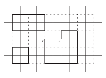
Figure 4.1. A configuration in $\mathcal{C}_{a}^{\uparrow}(z)$. The winding in the picture is $\mathbf{W}(\gamma:a\rightarrow z)=-2\pi$.

The Ising parafermionic observables are s-holomorphic and satisfy the Riemann boundary conditions, with a discrete singularity at $z=a$. To give a more precise statement, we first define a notion of discrete residue.

Definition 20.

Let $a$ be a horizontal edge. For a function $z\mapsto f(z)$ that is (massive) s-holomorphic for $z\neq a$ in a domain containing the faces $a\pm\frac{\mathfrak{i}}{2}$, the discrete residue of $f$ at $a$ is ${\rm Res}_{a}(f)=\frac{\mathfrak{i}}{2\pi}\left(f^{{\rm front}}(a)-f^{{\rm back}}(a)\right)$, where $f^{{\rm front}}(a)$ is such that if $f$ is extended to $a$ by this value, then $f$ becomes (massive) s-holomorphic on the face $a+\frac{\mathfrak{i}}{2}$, and $f^{{\rm back}}(a)$ is such that if $f$ is extended to $a$ by this value, then $f$ becomes (massive) s-holomorphic on the face $a-\frac{\mathfrak{i}}{2}$.

Proposition 21 ([Hon10a]).

Let $a\in\mathbf{I}^{*}\times\mathbf{J}$. If $a$ is not on the boundary, $a\in\mathbf{I}^{*}\times(\mathbf{J}\setminus\partial\mathbf{J})$, then the Ising parafermionic observables $f_{a}^{\uparrow}$ and $f_{a}^{\downarrow}$ are functions defined on edges $z\neq a$ such that

• $z\mapsto f_{a}^{\uparrow}(z)$ and $z\mapsto f_{a}^{\downarrow}(z)$ are massive s-holomorphic

• $f_{a}^{\uparrow}$ and $f_{a}^{\downarrow}$ satisfy RBVP: for $z$ a boundary edge of the rectangle $f_{a}^{\uparrow}(z)\in\mathbb{R}\tau_{{\rm cw}}^{-\frac{1}{2}}$ and $f_{a}^{\downarrow}(z)\in\mathbb{R}\tau_{{\rm cw}}^{-\frac{1}{2}}$

• the discrete residue of $f_{a}^{\uparrow}$ at $a$ is $\frac{\mathfrak{i}}{2\pi}$ and the discrete residue of $f_{a}^{\downarrow}$ at $a$ is $\frac{-1}{2\pi}$.

If $a$ is on the bottom boundary, $a\in\mathbf{I}_{0}^{*}$, then $f_{a}^{\downarrow}$ is zero and $f_{a}^{\uparrow}$ is a function defined on edges $z\neq a$ such that

• $z\mapsto f_{a}^{\uparrow}(z)$ becomes s-holomorphic in the whole domain with the definition $f_{a}^{\uparrow}(a)=1$

• $f_{a}^{\uparrow}$ and satisfies RBVP: for $z$ a boundary edge of the rectangle $f_{a}^{\uparrow}(z)\in\mathbb{R}\tau_{{\rm cw}}^{-\frac{1}{2}}$.

If $a$ is on the top boundary , $a\in\mathbf{I}_{N}^{*}$, similar statements hold.

The parafermionic observables can be defined similarly in any square lattice domain [HoSm10b]. At the critical point, $\beta=\beta_{c}$, one can treat scaling limits as follows. Take the domains to be subgraphs $\Omega_{\delta}$ of the square lattice $\delta\mathbb{Z}^{2}$ with small mesh $\delta$, approximating a given continuous domain $\Omega$ as $\delta\searrow 0$. The analogue of the above Proposition holds. The convergence of the parafermionic observables as $\delta\searrow 0$ can be controlled [HoSm10b, Hon10a]: the functions $f_{a}^{\uparrow}$ and $f_{a}^{\downarrow}$ divided by $\delta$ converge uniformly on compact subsets of $\Omega\setminus\left\{a\right\}$ to the unique holomorphic function with Riemann boundary values and the appropriate residue. By Theorems 22 and 23 below, we can deduce from this also the convergence in the scaling limit of the renormalized fermion correlation functions.

4.3.2. Fermion operator two-point correlation functions

Theorem 22.

We have

$$\left\langle\psi(z)\psi(a)\right\rangle_{\mathbf{I}\times\mathbf{J}}=\; -f_{a}^{\uparrow}(z)+\mathfrak{i}\,f_{a}^{\downarrow}(z)$$

$$\left\langle\psi(z)\bar{\psi}(a)\right\rangle_{\mathbf{I}\times\mathbf{J}}=\; \phantom{-}f_{a}^{\uparrow}(z)+\mathfrak{i}\,f_{a}^{\downarrow}(z)$$

$$=\; -\overline{f_{z}^{\uparrow}(a)}-\mathfrak{i}\,\overline{f_{z}^{\downarrow}(a)}$$

$$\left\langle\bar{\psi}(z)\bar{\psi}(a)\right\rangle_{\mathbf{I}\times\mathbf{J}}=\; -\overline{f_{a}^{\uparrow}(z)}-\mathfrak{i}\,\overline{f_{a}^{\downarrow}(z)}.$$

Proof.

Note that because of the relations of Theorem 19 and the fact that $f_{a}^{\uparrow/\downarrow}$ are massive s-holomorphic, it suffices to prove the statements when $z$ is a horizontal edge. Denote $z=x+\mathfrak{i}y$ and $a=x^{\prime}+\mathfrak{i}y^{\prime}$. Suppose for simplicity first that $y>y^{\prime}$. Consider the numerator of the second correlation function,

$$\langle\mathbf{e}_{(+)}|V^{N-y}\psi_{x}V^{y-y^{\prime}}\bar{\psi}_{x^{\prime}}V^{y^{\prime}}|\mathbf{e}_{(+)}\rangle$$

Expand the matrix product in the basis $(\mathbf{e}_{\sigma})$. Note that for any given $\sigma\in\left\{\pm 1\right\}^{\mathbf{I}}$ the matrix elements $\left(\bar{\psi}_{x^{\prime}}\right)_{\tau\sigma}$ and $\left(\psi_{x}\right)_{\tau\sigma}$ are non-zero only if $\tau$ is obtained from $\sigma$ by flipping the spins on the left of $x^{\prime}$ or $x$. The expansion is

$$\langle\mathbf{e}_{(+)}|V^{N-y}\psi_{x}V^{y-y^{\prime}}\bar{\psi}_{x^{\prime}}V^{y^{\prime}}|\mathbf{e}_{(+)}\rangle$$

$$=\; \mathrm{const.}\times\sum V_{(+),\sigma^{(N-1)}}V_{\sigma^{(N-1)},\sigma^{(N-2)}}V_{\sigma^{(N-2)},\sigma^{(N-3)}}\cdots$$

$$\qquad\qquad\cdots V_{\sigma^{(y+1)},\tau^{(y)}}\left(\psi_{x}\right)_{\tau^{(y)},\sigma^{(y)}}V_{\sigma^{(y)},\sigma^{(y-1)}}\cdots$$

$$\qquad\qquad\cdots V_{\sigma^{(y^{\prime}+1)},\tau^{(y^{\prime})}}\left(\bar{\psi}_{x^{\prime}}\right)_{\tau^{(y^{\prime})},\sigma^{(y^{\prime})}}V_{\sigma^{(y^{\prime})},\sigma^{(y^{\prime}-1)}}\cdots$$

$$\qquad\qquad\cdots V_{\sigma^{(3)},\sigma^{(2)}}V_{\sigma^{(2)},\sigma^{(1)}}V_{\sigma^{(1)},(+)}.$$

where the sum is over indices $\sigma^{(1)},\sigma^{(2)},\ldots,\sigma^{(N-1)}\in\left\{\pm 1\right\}^{\mathbf{I}}$ and the flipped spin configurations are

$$\tau_{j}^{(y)}=\; \begin{cases}\phantom{-}\sigma_{j}^{(y)}\quad&\text{for }j>x\\ -\sigma_{j}^{(y)}\quad&\text{for }j<x.\end{cases} \tau_{j}^{(y^{\prime})}=\; \begin{cases}\phantom{-}\sigma_{j}^{(y^{\prime})}\quad&\text{for }j>x^{\prime}\\ -\sigma_{j}^{(y^{\prime})}\quad&\text{for }j<x^{\prime}.\end{cases}$$

For the matrix elements of $V$ use the formula

$$V_{\rho\sigma}=\; e^{\frac{\beta}{2}\sum_{k\in\mathbf{I}^{*}}\rho_{k-\frac{1}{2}}\rho_{k+\frac{1}{2}}}\times e^{\beta\sum_{j\in\mathbf{I}}\sigma_{j}\rho_{j}}\times e^{\frac{\beta}{2}\sum_{k\in\mathbf{I}^{*}}\sigma_{k-\frac{1}{2}}\sigma_{k+\frac{1}{2}}}$$

$$=\; \mathrm{const.}\times\alpha^{\frac{1}{2}\,\#\{k\,|\,\rho_{k-\frac{1}{2}}\neq\rho_{k+\frac{1}{2}}\}}\;\alpha^{\#\{j\,|\,\sigma_{j}\neq\rho_{j}\}}\;\alpha^{\frac{1}{2}\,\#\{k\,|\,\sigma_{k-\frac{1}{2}}\neq\sigma_{k+\frac{1}{2}}\}},$$

where $\alpha=e^{-2\beta}$. In most rows, we can combine the factors from the matrix elements of two $\left(V^{{\rm h}}\right)^{\frac{1}{2}}$ to just one factor. The sum essentially amounts to summing over spin configurations in the entire box, except from the peculiarity that in rows $y$ and $y^{\prime}$ we have two configurations related to each other by flipping the spins on the left of $x$ or $x^{\prime}$. Thus the terms in the sum correspond to contours $\gamma\in\mathcal{C}_{a}^{\uparrow}(z)\cup\mathcal{C}_{a}^{\downarrow}(z)$ by the rule that a dual edge is in $\gamma$ if it separates two spins of opposite value: in rows $y$ and $y^{\prime}$ the two flipped configurations amount for half-edges arriving to the points $z=x+\mathfrak{i}y$ and $a=x^{\prime}+\mathfrak{i}y^{\prime}$. The half edge in row $y$ has two possible directions. The half-edge is either from $x+\mathfrak{i}y$ to the face $x+\mathfrak{i}(y+\frac{1}{2})$ above (resp. the face $x+\mathfrak{i}(y-\frac{1}{2})$ below) if $\sigma_{x+\frac{1}{2}}^{(y)}=\sigma_{x-\frac{1}{2}}^{(y)}$ and $\tau_{x+\frac{1}{2}}^{(y)}\neq\tau_{x-\frac{1}{2}}^{(y)}$ (resp. $\sigma_{x+\frac{1}{2}}^{(y)}\neq\sigma_{x-\frac{1}{2}}^{(y)}$ and $\tau_{x+\frac{1}{2}}^{(y)}=\tau_{x-\frac{1}{2}}^{(y)}$) and in this case we set $\eta=+1$ (resp. $\eta=-1$). Similarly we set $\eta^{\prime}=+1$ or $\eta^{\prime}=-1$ if the half edge in row $y^{\prime}$ is from $x^{\prime}+\mathfrak{i}y^{\prime}$ to the face above or below, respectively, i.e. if $\sigma_{x^{\prime}+\frac{1}{2}}^{(y^{\prime})}=\sigma_{x^{\prime}-\frac{1}{2}}^{(y^{\prime})}$ or $\sigma_{x^{\prime}+\frac{1}{2}}^{(y^{\prime})}\neq\sigma_{x^{\prime}-\frac{1}{2}}^{(y^{\prime})}$, respectively. The matrix elements of all $V$ together produce a factor $\alpha^{L(\gamma)}$ times a constant. The matrix element of $\psi_{x}$ produces the complex factor $\mathfrak{i}(-1)^{\#(\gamma\cap\mathbf{I}_{y}^{>x})}\lambda^{\eta}$, where $\#(\gamma\cap\mathbf{I}_{y}^{>x})$ is the number of edges of the contour $\gamma$ on row $y$ on the right of $x$ and $\lambda=e^{\mathfrak{i}\pi/4}$. Similarly the matrix element of $\bar{\psi}_{x^{\prime}}$ produces the complex factor $(-1)^{\#(\gamma\cap\mathbf{I}_{y^{\prime}}^{>x^{\prime}})}\lambda^{-\eta^{\prime}}$. We now write the result of the expansion in terms of sum over contours,

$$\langle\mathbf{e}_{(+)}|V^{N-y}\psi_{x}V^{y-y^{\prime}}\bar{\psi}_{x^{\prime}}V^{y^{\prime}}|\mathbf{e}_{(+)}\rangle$$

$$=\; \mathrm{const.}\times\mathfrak{i}\sum_{\gamma\in\mathcal{C}_{a}^{\uparrow}(z)\cup\mathcal{C}_{a}^{\downarrow}(z)}\alpha^{L(\gamma)}(-1)^{\#(\gamma\cap\mathbf{I}_{y}^{>x})+\#(\gamma\cap\mathbf{I}_{y^{\prime}}^{>x^{\prime}})}\lambda^{\eta-\eta^{\prime}}.$$

Combinatorial considerations of the topological possibilities for the curve in $\gamma$ from $a$ to $z$ show that $(-1)^{\#(\gamma\cap\mathbf{I}_{y}^{>x})+\#(\gamma\cap\mathbf{I}_{y^{\prime}}^{>x^{\prime}})}\lambda^{\eta-\eta^{\prime}}=-\mathfrak{i}e^{-\frac{\mathfrak{i}}{2}\mathbf{W}(\gamma:a\rightarrow z)}$, where $\mathbf{W}(\gamma:a\rightarrow z)$ is the winding of the path as in the definition of the parafermionic observable (note a difference to the case $y<y^{\prime}$: we would have $(-1)^{\#(\gamma\cap\mathbf{I}_{y}^{>x})+\#(\gamma\cap\mathbf{I}_{y^{\prime}}^{>x^{\prime}})}\lambda^{\eta-\eta^{\prime}}=\mathfrak{i}e^{-\frac{\mathfrak{i}}{2}\mathbf{W}(\gamma:a\rightarrow z)}$ instead). Thus we write our final expression for the numerator of the second correlation function,

$$\langle\mathbf{e}_{(+)}|V^{N-y}\psi_{x}V^{y-y^{\prime}}\bar{\psi}_{x^{\prime}}V^{y^{\prime}}|\mathbf{e}_{(+)}\rangle$$

$$=\; \mathrm{const.}\times\sum_{\gamma\in\mathcal{C}_{a}^{\uparrow}(z)\cup\mathcal{C}_{a}^{\downarrow}(z)}\alpha^{L(\gamma)}e^{-\frac{\mathfrak{i}}{2}\mathbf{W}(\gamma:a\rightarrow z)}.$$

The denominator is $\langle\mathbf{e}_{(+)}|V^{N}|\mathbf{e}_{(+)}\rangle=\mathrm{const.}\times\mathcal{Z}$ with the same multiplicative constant (here $\mathcal{Z}$ is as in Section 4.3.1), so we get the expression

$$\left\langle\psi(z)\bar{\psi}(a)\right\rangle=\; f_{a}^{\uparrow}(z)+\mathfrak{i}\,f_{a}^{\downarrow}(z).$$

In the case $y<y^{\prime}$, before we do the expansion of the matrix product, we must anticommute $\psi(z)$ to the right of $\bar{\psi}(a)$, which gives an overall sign difference. This is nevertheless cancelled in the end result by another opposite sign resulting from the combinatorial considerations of topological possibilities for the curve $\gamma$.

For the first correlation function, a similar consideration gives when $y>y^{\prime}$,

$$\langle\mathbf{e}_{(+)}|V^{N-y}\psi_{x}V^{y-y^{\prime}}\psi_{x^{\prime}}V^{y^{\prime}}|\mathbf{e}_{(+)}\rangle$$

$$=\; \mathrm{const.}\times(-1)\sum_{\gamma\in\mathcal{C}_{a}^{\uparrow}(z)\cup\mathcal{C}_{a}^{\downarrow}(z)}\alpha^{L(\gamma)}(-1)^{\#(\gamma\cap\mathbf{I}_{y}^{>x})+\#(\gamma\cap\mathbf{I}_{y^{\prime}}^{>x^{\prime}})}\lambda^{\eta+\eta^{\prime}}.$$

In this case we have $(-1)^{\#\gamma\cap\mathbf{I}_{y}^{>x}+\#\gamma\cap\mathbf{I}_{y^{\prime}}^{>x^{\prime}}}\lambda^{\eta+\eta^{\prime}}=\eta^{\prime}e^{-\frac{\mathfrak{i}}{2}\mathbf{W}(\gamma:a\rightarrow z)}$, leading to

$$\left\langle\psi(z)\psi(a)\right\rangle=\; -f_{a}^{\uparrow}(z)+\mathfrak{i}\,f_{a}^{\downarrow}(z).$$

∎

4.4. Pfaffian formulas for multi-point fermion correlation functions

The multi-point correlation functions of the fermions can be written in terms of two-point correlation functions. Recall the abbreviated notation of Section 4 for fermion correlation functions — in particular each $\psi^{(i)}$ in the statement below can be either $\psi$ or $\bar{\psi}$.

Theorem 23.

We have

$$\left\langle\psi^{(1)}(z_{1})\cdots\psi^{(n)}(z_{n})\right\rangle_{\mathbf{I}\times\mathbf{J}}^{+}=\; \mathrm{Pf}\left(\left[\left\langle\psi^{(i)}(z_{i})\psi^{(j)}(z_{j})\right\rangle_{\mathbf{I}\times\mathbf{J}}^{+}\right]_{i,j=1}^{n}\right).$$

Proof.

We use the polarization of Lemma 15, which works for all $\beta>0$ except possibly isolated values, and since both sides of the asserted equation are analytic as functions of $\beta$, the statement will be proven for all $\beta$. By the aforementioned lemma, the state $v_{{\rm vac}}=\mathbf{e}_{(+)}$ is a vacuum of the Fock space $\mathcal{S}_{+}\cong\bigwedge\mathcal{W}_{\boxplus}^{(+);N}$, and the mapping

$$u\mapsto\; \frac{1}{\mathbf{e}_{(+)}^{\top}V^{N}\mathbf{e}_{(+)}}\mathbf{e}_{(+)}^{\top}V^{N}u=\left\langle v_{{\rm vac}}^{*},\,u\right\rangle$$

defines the dual vacuum $v_{{\rm vac}}^{*}\in\left(\bigwedge\mathcal{W}_{\boxplus}^{(+);N}\right)^{*}$. The denominator in the definition of correlation functions in Section 4 is the same as the denominator in the above formula for the dual vacuum, $\langle\mathbf{e}_{(+)}|V^{N}|\mathbf{e}_{(+)}\rangle=\mathbf{e}_{(+)}^{\top}V^{N}\mathbf{e}_{(+)}$. The correlation functions thus read $\left\langle\psi^{(1)}(z_{1})\cdots\psi^{(n)}(z_{n})\right\rangle_{\mathbf{I}\times\mathbf{J}}^{+}=\left\langle v_{{\rm vac}}^{*},\,\psi^{(1)}(z_{1})\cdots\psi^{(n)}(z_{n})v_{{\rm vac}}\right\rangle$. Finally note that $\psi^{(i)}(z_{i})\in\mathcal{W}$ for all $i=1,2,\ldots,n$, so the statement follows from the fermionic Wick’s formula, Lemma 12, applied to the polarization $\mathcal{W}=\mathcal{W}_{\boxplus}^{(+);t}\oplus\mathcal{W}_{\boxminus}^{(+);t}$ of Lemma 15. ∎

4.5. Multipoint Ising parafermionic observables

Let us now define multipoint parafermionic observables introduced in [Hon10a]. Let $\Omega$ be a square grid domain, with dual $\Omega^{*}$ consisting of the faces. Denote the set of edges of $\Omega$ by $\mathcal{E}$ and the set of dual edges by $\mathcal{E}^{*}$. Let $z_{1},\ldots,z_{2m}$ be (midpoints of) edges, and for each $z_{j}$, let $o_{j}$ be a choice of orientation of the corresponding dual edge $e_{j}^{*}$ (i.e. $o_{j}\in\left\{\pm 1\right\}$ if $e_{j}^{*}$ is horizontal and $o_{j}\in\left\{\pm i\right\}$ if $e_{j}^{*}$ is vertical), and let $\varepsilon_{j}\in\mathbb{C}$ be choices of square roots of the orientations, $\varepsilon_{j}^{2}=o_{j}$.

We define the multipoint observable $f^{\epsilon}\left(z_{1},\ldots,z_{2m}\right)$ by

$$f^{\varepsilon}\left(z_{1},\ldots,z_{2m}\right)=\sum_{\gamma\in\mathcal{C}_{z_{1},\ldots,z_{2m}}^{\varepsilon}}\alpha^{L(\gamma)}\;\mathrm{sign}\left(\gamma\right)\prod_{\pi_{j}:z_{s_{j}}\leadsto z_{d_{j}}}\frac{\varepsilon_{d_{j}}}{\varepsilon_{s_{j}}}e^{-\mathfrak{i}\mathbf{W}\left(\pi_{j}\right)},$$

where

• $\mathcal{C}_{z_{1},\ldots,z_{2m}}^{\varepsilon}$ is the set of $\gamma\subset\mathcal{E}^{*}$ consisting of the (dual) half edges $<z_{j},z_{j}+\frac{o_{j}}{2}>$ and of (dual) edges of $\mathcal{E}^{*}$ such that each vertex $p\in\Omega^{*}$ belongs to an even number of edges/half edges of $\gamma$: in other words a configuration $\gamma$ contains loops and $m$ paths $\pi_{1},\ldots,\pi_{m}$ linking pairwise the $z_{j}$’s. By $L(\gamma)$ we mean the number of edges of $\mathcal{E}^{*}$ in $\gamma$ plus $m$, with the additional $m$ accounting for the $2m$ half edges.

• The product is over the $m$ paths $\pi_{1},\ldots,\pi_{m}$, where each $\pi_{j}$ is oriented from $z_{s_{j}}$ to $z_{d_{j}}$ where $s_{j}<d_{j}$ (i.e. we orient the paths from smaller to greater indices).

• $\mathrm{sign}\left(\gamma\right)=\left(-1\right)^{\#\mathrm{crossings}}$, where $\#\mathrm{crossings}$ is the number of crossings of the pair partition $\left\{\left\{s_{j},d_{j}\right\}:j\in\left\{1,\ldots,m\right\}\right\}$ of $\left\{1,\ldots,2m\right\}$ induced by the paths $\pi_{1},\ldots,\pi_{m}$ ($\pi_{j}$ from $z_{s_{j}}$ to $z_{d_{j}}$), i.e. the number of 4-tuples $s_{j}<d_{j}<s_{k}<d_{k}$.

• It can be checked [Hon10a] that if there are ambiguities in the choices of paths $\pi_{1},\ldots,\pi_{n}$, the weight of a configuration $\gamma$ is independent of the way that they are resolved, provided that wherever there is an ambiguity each path turns left or right (going straight is forbidden).

The observables $f^{\epsilon}\left(z_{1},\ldots,z_{2m}\right)$ can be used to compute the scaling limit of the energy density correlations, as well as boundary spin correlations with free boundary conditions (see [Hon10a]). The key property that allows one to study the observable at criticality is its s-holomorphicity:

Proposition 24 ([Hon10a]).

Let $o_{1},\ldots,o_{2m-1}\in\mathbb{C}$ be orientations of edges $e_{1}^{*},\ldots,e_{2m-1}^{*}$ and let $\varepsilon_{1},\ldots,\varepsilon_{2m-1}\in\mathbb{C}$ be such that $\varepsilon_{1}^{2}=o_{1},\ldots,\varepsilon_{2m-1}^{2}=o_{2m-1}$. Let $z_{1},\ldots,z_{2m-1}$ be the midpoints of $e_{1}^{*},\ldots,e_{2m-1}^{*}$. For any midpoint of edge $z_{2m}$, let $o_{2m}$ and $o_{2m}$ be its two possible orientations, let $\varepsilon_{2m}$ and $\tilde{\varepsilon}_{2m}$ be such that $\varepsilon_{2m}^{2}=o_{2m}$ and $\tilde{\varepsilon}_{2m}^{2}:=-o_{2m}$, and let $\varepsilon:=\left(\varepsilon_{1},\ldots,\varepsilon_{2m}\right)$ and $\tilde{\varepsilon}:=\left(\varepsilon_{1},\ldots,\varepsilon_{2m-1},\tilde{\varepsilon}_{2m}\right)$.

Then we have that $g\left(z_{2m}\right):=\frac{\lambda}{\varepsilon_{2m}}f^{\varepsilon}\left(z_{1},\ldots,z_{2m}\right)+\frac{\lambda}{\tilde{\varepsilon}_{2m}}f^{\tilde{\varepsilon}}\left(z_{1},\ldots,z_{2m}\right)$ is independent of the choice of $\varepsilon_{2m},\tilde{\varepsilon}_{2m}$ and at criticality $z_{2m}\mapsto g\left(z_{2m}\right)$ is s-holomorphic on $\Omega\setminus\left\{z_{1},\ldots,z_{2m-1}\right\}$, with $\parallel\tau_{\mathrm{cw}}^{-\frac{1}{2}}$ boundary conditions.

As for the fermion operator two point correlation functions and two point parafermionic observables, it is true that the fermion operator multipoint correlation functions are expressible as linear combinations of the multipoint parafermionic observables and vice versa.

Theorem 25.

Define $\psi^{\uparrow}(z)=\frac{1}{2}(\bar{\psi}(z)-\psi(z))$ and $\psi^{\downarrow}(z)=\frac{\mathfrak{i}}{2}(\psi(z)+\bar{\psi}(z))$. Then we have

$$\left\langle\psi^{\updownarrow_{2m}}(z_{2m})\cdots\psi^{\updownarrow_{1}}(z_{1})\right\rangle_{\mathbf{I}\times\mathbf{J}}^{+}=\; f^{\varepsilon}(z_{1},\ldots,z_{2m}),$$

where the arrows $\updownarrow_{j}\in\left\{\uparrow,\downarrow\right\}$ and the square roots of directions $\varepsilon_{j}=\sqrt{o_{j}}$ are chosen as follows

$$\begin{cases}\varepsilon_{j}=\lambda\quad&\text{if }\updownarrow_{j}=\uparrow\\ \varepsilon_{j}=\lambda^{-3}\quad&\text{if }\updownarrow_{j}=\downarrow\end{cases} \;.$$

Proof.

Suppose for simplicity that $z_{j}=x_{j}+\mathfrak{i}y_{j}$ with $y_{1}<y_{2}<\cdots<y_{2m}$. Form a low temperature expansion of the fermion operator correlation function as in the proof of Theorem 22. Consider any fixed $j=1,2,\ldots,2m$. Adding up the low temperature expansions of the two terms in the definition of $\psi^{\updownarrow_{j}}(z_{j})$ we get that the total weight for the configurations where the half edge from $z_{j}$ to $z_{j}+\frac{1}{2}\eta_{j}\mathfrak{i}$ is used ($\eta_{j}\in\left\{\pm 1\right\}$) is used is in the two cases $\updownarrow_{j}=\uparrow$ and $\updownarrow_{j}=\downarrow$ respectively proportional to $\frac{1}{2}(\lambda^{-\eta_{j}}-\mathfrak{i}\lambda^{\eta_{j}})=\lambda^{-1}\delta_{\eta_{j},+1}$ and $\frac{\mathfrak{i}}{2}(\mathfrak{i}\lambda^{\eta_{j}}+\lambda^{-\eta_{j}})=\lambda^{3}\delta_{\eta_{j},-1}$, where the Kronecker deltas in particular ensure that only the contributions of the contours $\mathcal{C}_{z_{1},\ldots,z_{2n}}^{\varepsilon}$ survive, as in the definition of the corresponding parafermionic multipoint observable. In the low temperature expansion, contours $\gamma$ always come have a factor $\alpha^{L(\gamma)}$ in their weight due to the product of matrix elements of $V^{{\rm h}}$ and $V^{{\rm v}}$, and for any surviving contour $\gamma\in\mathcal{C}_{z_{1},\ldots,z_{2n}}^{\varepsilon}$ the remaining phase factor coming from the matrix elements of $\left(\psi_{x_{j}}^{\updownarrow_{j}}\right)$ equals ${\rm sgn}({\rm pairing}(\gamma))\times\prod_{p=1}^{m}\frac{\varepsilon_{d_{p}}}{\varepsilon_{s_{p}}}$. ∎

As a direct consequence of Theorems 23 and 25, we get a Pfaffian formula for the multi-point parafermionic observables.

Corollary 26.

Let $e_{1}^{*},\ldots,e_{2n}^{*}$ be dual edges with orientations $o_{1},\ldots,o_{2n}$ and let $\varepsilon_{1},\ldots,\varepsilon_{2n}$ be such that $\varepsilon_{1}^{2}=o_{1},\ldots,\varepsilon_{2n}^{2}=o_{2n}$. Then we have that

$$f^{\varepsilon}\left(z_{1},\ldots,z_{2n}\right)=\mathrm{Pfaff}\left(f^{\left(\varepsilon_{j},\varepsilon_{k}\right)}\left(z_{j},z_{k}\right)\mathbf{1}_{j\neq k}\right)_{1\leq j,k\leq 2n}.$$

This formula was proved in [Hon10a] in the critical case $\beta=\beta_{c}$ for domains of arbitrary shape, by verifying that the s-holomorphic function in Proposition 24 satisfies a discrete Riemann boundary value problem with singularities, which uniquely characterizes the parafermionic observable. The special case which gives the Ising model boundary spin correlation functions with free boundary conditions was proven by direct combinatorial methods in [GBK78, KLM12] for very general classes of planar graphs. Our approach works at any $\beta$, but for the Ising model on square lattice only, and for domains of general shape some minor technical modifications are needed in the proof: the domain should be thought of as a subgraph of a large rectangle $\mathbf{I}\times\mathbf{J}$, and for every row the transfer matrix should be replaced by a composition of $V$ and a projection which enforces plus boundary conditions outside the domain. Nevertheless, we believe that our approach in conceptually the clearest, as the Pfaffian appears simply because of the fermionic Wick’s formula (Lemma 12). This illustrates an advantage of the operator formalism, some algebraic structures underlying the Ising model are more evident and can be better exploited.

4.6. Correlation functions of the fermion and spin operators

It is also possible to consider correlation functions of fermion operators and spin operators simultaneously. It turns out that as functions of the fermion operator positions, these become branches of multivalued observables. For example, when $a\in\mathbf{I}_{0}^{*}$ is on the bottom side of the rectangle and $w_{1},\ldots,w_{n}\in\mathbf{I}\times\mathbf{J}$,

$$z\mapsto \frac{\left\langle\psi(z)\bar{\psi}(a)\hat{\sigma}(w_{1})\cdots\hat{\sigma}(w_{n})\right\rangle_{\mathbf{I}\times\mathbf{J}}^{+}}{\left\langle\hat{\sigma}(w_{1})\cdots\hat{\sigma}(w_{n})\right\rangle_{\mathbf{I}\times\mathbf{J}}^{+}}=\frac{\langle\mathbf{e}_{(+)}|V^{N}\psi(z)\bar{\psi}(a)\hat{\sigma}(w_{1})\cdots\hat{\sigma}(w_{n})|\mathbf{e}_{(+)}\rangle}{\langle\mathbf{e}_{(+)}|V^{N}\hat{\sigma}(w_{1})\cdots\hat{\sigma}(w_{n})|\mathbf{e}_{(+)}\rangle}$$

becomes a (massive) s-holomorphic function in the complement of the branch cuts starting from each $w_{j}\in\mathbf{I}\times\mathbf{J}$ to the right boundary of the rectangle. The function can be extended to the branch cut in two ways, one of which satisfies (massive) s-holomorphicity conditions on the faces below the cut and another which satisfies them on the faces above the cut — the two definitions differ by a sign, indicating a square root type monodromy of the function at the locations $w_{j}$ of the spin insertions. A low temperature expansion like in the proofs of Theorems 22 and 25 shows that this function is a branch of the parafermionic spinor observable of [ChIz11, CHI12], where the observable is properly defined on a double covering of the punctured lattice domain in order to obtain a well defined s-holomorphic function.

5. Operators on Cauchy data spaces

As explained above, the Ising transfer matrix can be constructed directly in terms of the s-holomorphic propagator (Sections 1.3.1 and 3.3). We now discuss s-holomorphic approaches to the data carried by the transfer matrix quantum states. In Sections 4.3 and 4.5, we learned the following:

• The correlation functions of the fermion operators can be expressed as linear combinations of parafermionic observables.

• The parafermionic observables can be characterized in s-holomorphic terms: they are the unique s-holomorphic functions with Riemann boundary values and prescribed singularities.

In this section, we present an s-holomorphic construction inspired by transfer matrix states. A quantum state $\mathcal{Q}\in\mathcal{S}$ living on a row $\mathbf{I}_{k}$ contains all the information about the geometry of the domain and the operator insertions below $\mathbf{I}_{k}$. Likewise, we construct discrete Riemann Poincaré-Steklov (RPS) operators living on a row (more generally, any crosscut of the domain), which act on Cauchy data spaces. These RPS operators together with the vectors on which they act contain all the information about the geometry of the domain and operator insertions. These operators can be written as convolution operators with parafermionic observables, which are fermion correlations and hence can be directly represented from the quantum states. They also can be propagated using explicit convolution operators.

A great advantage of the discrete RPS operators is that they have nice scaling limits, as singular integral operators, and that they work in arbitrary planar geometries.

5.1. Discrete RPS operators

In this Section, we define the Riemann Poincaré-Steklov operators.

Let $\Omega$ be a square grid domain, let $\mathfrak{b}\subset\partial\mathcal{E}$ be a collection of boundary edges and $\mathcal{R}_{\Omega}^{\mathfrak{b}}$ and be the space of functions $f:\mathfrak{b}\to\mathbb{C}$ such that $f\parallel\tau_{\mathrm{ccw}}^{-\frac{1}{2}}$ on $\mathfrak{b}$. Let $\mathcal{I}_{\Omega}^{\mathfrak{b}}$ be the space of functions $f:\mathfrak{b}\to\mathbb{C}$ such that $f\parallel\tau_{\mathrm{cw}}^{-\frac{1}{2}}$ on $\mathfrak{b}$.

First, we state a key lemma, which guarantees the uniqueness of solutions to Riemann boundary value problems.

Lemma 27.

Let $\Omega$ be a square grid domain with edges $\mathcal{E}$. If $h:\mathcal{E}\to\mathbb{C}$ is an s-holomorphic function with $h\parallel\tau_{\mathrm{cw}}^{-\frac{1}{2}}$ on $\partial\mathcal{E}$, then $h=0$.

Proof.

The proof of this lemma is given in [Hon10a, Corollary 29] (where the notion of s-holomorphicity comes with a phase change of $e^{\mathfrak{i}\pi/4}$ compared to the present paper). The idea is to show that for any s-holomorphic function $g:\mathcal{E}\to\mathbb{C}$ with boundary values $u+v$, where $u\in\mathcal{R}_{\Omega}^{\mathfrak{b}}$ and $v\in\mathcal{I}_{\Omega}^{\mathfrak{b}}$, we have that $\sum_{z\in\mathfrak{b}}\left|v\left(z\right)\right|^{2}\leq\sum_{z\in\mathfrak{b}}\left|u\left(z\right)\right|^{2}$ (the proof of this inequality relies on the definition of a discrete analogue of $\Im\mathfrak{m}\int g^{2}$). In our case $u=0$, and hence $v=0$ as well. ∎

Lemma 28.

For any $u\in\mathcal{R}_{\Omega}^{\mathfrak{b}}$, there exists a unique $v\in\mathcal{I}_{\Omega}^{\mathfrak{b}}$ such that $u+v$ has an s-holomorphic extension $h:\mathcal{E}\to\mathbb{C}$ satisfying $h\parallel\tau_{\mathrm{cw}}^{-\frac{1}{2}}$ on $\partial\Omega\setminus\mathfrak{b}$.

Proof.

For any $v\in\mathcal{I}_{\Omega}^{\mathfrak{b}}$, there exists at most one $u\in\mathcal{R}_{\Omega}^{\mathfrak{b}}$ such that $u+v$ has an s-holomorphic extension $h$ to $\Omega\to\mathbb{C}$ with $\parallel\tau_{\mathrm{cw}}^{-\frac{1}{2}}$ on $\partial\mathcal{E}\setminus\mathfrak{b}$: if we suppose there are two extensions, their difference will satisfy the boundary condition $\parallel\tau_{\mathrm{cw}}^{-\frac{1}{2}}$ on $\partial\mathcal{E}$ and hence be $0$ by Lemma 27. By a dimensionality argument, there exists exactly one such $u$ and the mapping $v\mapsto u$ is an invertible linear map. ∎

Definition 29.

We define the RPS operator $U_{\Omega}^{\mathfrak{b}}:\mathcal{R}_{\Omega}^{\mathfrak{b}}\to\mathcal{I}_{\Omega}^{\mathfrak{b}}$ as the mapping $u\mapsto v$ defined by Lemma 30 (which is an isomorphism by the proof).

Lemma 30.

With the notation of Lemma 28, we have that

(5.1) $$v\left(x\right) = \sum_{y\in\mathfrak{b}\setminus\left\{x\right\}}u\left(y\right)f_{\Omega}\left(y,x\right)\quad\forall x\in\partial\mathcal{E}$$

and the s-holomorphic extension $h$ is given by

(5.2) $$h\left(x\right)=\sum_{y\in\mathfrak{b}}u\left(y\right)f_{\Omega}\left(y,z\right)\quad\forall x\in\mathcal{E}.$$

Remark.

The convolution formula, Equation (5.2), is the key to pass to the scaling limit: the kernel $f_{\Omega}$ converges to a kernel of a continuous singular integral operator (see [HoKy11, Section 13]).

Proof.

Let us first notice that (5.2) implies (5.1): if $x\in\partial\mathcal{E}$, we have $u\left(x\right)f_{\Omega}\left(x,x\right)\in\tau_{\mathrm{ccw}}^{-\frac{1}{2}}$ and $u\left(y\right)f_{\Omega}\left(y,x\right)\in\tau_{\mathrm{cw}}^{-\frac{1}{2}}\left(y\right)$ for $y\in\partial\mathcal{E}\setminus\left\{x\right\}$, and hence the projection of (5.2) on $\mathcal{I}$ is indeed (5.1).

To prove (5.2), notice that the right-hand side is an s-holomorphic function, with the right boundary conditions (i.e. the same as $h$ in Lemma 28). The difference of both sides must then be $0$, by Lemma 27. ∎

In rectangular boxes, the RPS operator can be written simply in terms of the s-holomorphic propagation

Lemma 31.

Let $\Omega$ be a rectangular box $\mathbf{I}\times\left\{0,\ldots,N\right\}$, let $\mathfrak{b}=\mathbf{I}\times\left\{0\right\}$ be the bottom side and let $P:\left(\mathbb{R}^{2}\right)^{\mathbf{I}^{*}}\to\left(\mathbb{R}^{2}\right)^{\mathbf{I}^{*}}$ be the s-holomorphic propagation as defined in Section 2.4. For $N\geq 0$, decompose the s-holomorphic propagation $P^{N}$ into four $\left|\mathbf{I}^{*}\right|\times\left|\mathbf{I}^{*}\right|$ blocks

$$P^{N}=\begin{pmatrix}P_{\Re\Re}^{N}&P_{\Re\Im}^{N}\\ P_{\Im\Re}^{N}&P_{\Im\Im}^{N}\end{pmatrix}$$

corresponding to the decomposition $\left(\mathbb{R}^{2}\right)^{\mathbf{I}^{*}}\cong\mathbb{R}^{\mathbf{I}^{*}}\oplus\mathfrak{i}\mathbb{R}^{\mathbf{I}^{*}}$ into real and imaginary parts. Then have

$$U_{\Omega}^{\mathfrak{b}} = -\left(P_{\Im\Im}^{N}\right)^{-1}P_{\Re\Im}^{N}.$$

Proof.

Let $u\in\mathcal{R}_{\Omega}^{\mathfrak{b}}$ (i.e. purely real in this case) and $v\in\mathcal{I}_{\Omega}^{\mathfrak{b}}$ be defined by $v=U_{\Omega}^{\mathfrak{b}}u$. By definition of $U_{\Omega}^{\mathfrak{b}}$, we have that

$$\begin{pmatrix}P_{\Re\Re}^{N}&P_{\Re\Im}^{N}\\ P_{\Im\Re}^{N}&P_{\Im\Im}^{N}\end{pmatrix}\begin{pmatrix}u\\ v\end{pmatrix}=\begin{pmatrix}w\\ 0\end{pmatrix}$$

for some purely real function $w:\mathbf{I}\times\left\{n\right\}\to\mathbb{R}$. Hence, we get that $P_{\Im\Re}^{N}u+P_{\Im\Im}^{N}v=0$. Since we know that for any $u\in\mathcal{R}_{\Omega}^{\mathfrak{b}}$, there exists a unique $v$ satisfying this equation (as $U_{\Omega}^{\mathfrak{b}}$ is an isomorphism), we get that $v=-\left(P_{\Im\Im}^{N}\right)^{-1}P_{\Re\Im}^{N}u$. ∎

5.2. RPS pairings

In this subsection, we explain how to pair together s-holomorphic data coming from two adjacent domains with disjoint interiors, using RPS operators and Ising parafermionic observables. A related discussion about discrete kernel gluings (in a different framework, without boundaries) can be found in [Dub11a]. In our framework, the gluing operation arises as an analogue of pairing of transfer matrix states.

Let us define the setup of this subsection. Let $\Omega_{1},\Omega_{2}$ be two adjacent square grid domains with disjoint interiors, with edges $\mathcal{E}_{1},\mathcal{E}_{2}$, let $\Omega:=\Omega_{1}\cup\Omega_{2}$ and assume that $\mathfrak{b}:=\partial\mathcal{E}_{1}\cap\partial\mathcal{E}_{2}$ is connected. Let $U_{1}:=U_{\Omega_{1}}^{\mathfrak{b}}$ and $U_{2}:=U_{\Omega_{2}}^{\mathfrak{b}}$ be the RPS operators defined in the previous subsection and set $\mathcal{R}_{j}:=\mathcal{R}_{\Omega_{j}}^{\mathfrak{b}}$ and $\mathcal{I}_{j}^{\mathfrak{b}}:=\mathcal{I}_{\Omega_{j}}^{\mathfrak{b}}$ for $j=1,2$. We have $\mathcal{R}_{1}=\mathcal{I}_{2}$ and $\mathcal{R}_{2}=\mathcal{I}_{1}$.

Lemma 32.

We have that $\left(\mathrm{Id}-U_{1}U_{2}\right):\mathcal{R}_{2}\to\mathcal{R}_{2}$ and $\left(\mathrm{Id}-U_{2}U_{1}\right):\mathcal{R}_{1}\to\mathcal{R}_{1}$ are isomorphisms.

Proof.

The injectivity (and hence the bijectivity) of these operators follows from the fact that if a function $u\in\mathcal{R}_{2}$ is a fixed point of $U_{1}U_{2}$, then $u+U_{2}u$ admits an s-holomorphic extension to $\Omega$ with boundary condition $\parallel\tau_{\mathrm{cw}}^{-\frac{1}{2}}$ on $\partial\mathcal{E}$, and is hence $0$ by Lemma 27. ∎

A useful corollary of the previous lemma is the following fixed point result:

Corollary 33.

Let $h_{1}\in\mathcal{I}_{1}$ and $h_{2}\in\mathcal{I}_{2}$. Then there exists a unique function $f:\mathcal{E}\to\mathbb{C}$ such that for $j=1,2$, the function $f-h_{j}$ has an s-holomorphic extension to $\mathcal{E}_{j}$ with boundary conditions $\parallel\tau_{\mathrm{cw}}^{-\frac{1}{2}}$ on $\partial\mathcal{E}_{j}$. We have that $f=u_{1}+u_{2}$, where $u_{1}$ and $u_{2}$ are given by

$$u_{1} = \left(\mathrm{Id}-U_{2}U_{1}\right)^{-1}\left(U_{2}h_{1}+h_{2}\right),$$

$$u_{2} = \left(\mathrm{Id}-U_{1}U_{2}\right)^{-1}\left(U_{1}h_{2}+h_{1}\right).$$

Proof.

Suppose first that there exists an $f$ such that the functions $f-h_{j}$ have s-holomorphic extensions to $\mathcal{E}_{j}$ with boundary conditions $\parallel\tau_{\mathrm{cw}}^{-\frac{1}{2}}$ on $\partial\mathcal{E}_{j}$. Set $f_{j}:=f-h_{j}$ and write $f_{j}=u_{j}+v_{j}$, where $u_{j}\in\mathcal{R}_{j}$ and $v_{j}\in\mathcal{I}_{j}$. We have that $f=u_{1}+u_{2}$ and

$$u_{1} = v_{2}+h_{2}=U_{2}u_{2}+h_{2}=U_{2}\left(v_{1}+h_{1}\right)+h_{2}=U_{2}U_{1}u_{1}+U_{2}h_{1}+h_{2}$$

$$u_{2} = v_{1}+h_{1}=U_{1}u_{1}+h_{1}=U_{1}\left(v_{2}+h_{2}\right)+h_{1}=U_{1}U_{2}u_{2}+U_{1}h_{2}+h_{1},$$

which gives that $\left(\mathrm{Id}-U_{2}U_{1}\right)u_{1}=U_{2}h_{1}+h_{2}$ and $\left(\mathrm{Id}-U_{1}U_{2}\right)u_{2}=U_{1}h_{2}+h_{1}$. By Lemma 32, we obtain the asserted formulas for $u_{1}$ and $u_{2}$, proving the uniqueness of $f$. For any $(h_{1},h_{2})$ we have seen that there is at most one and hence exactly one solution $(u_{1},u_{2})$ of the equations

$$\left[\begin{array}[]{cc}U_{1}&-\mathrm{id}\\ -\mathrm{id}&U_{2}\end{array}\right]\left[\begin{array}[]{c}u_{1}\\ u_{2}\end{array}\right]=\; \left[\begin{array}[]{c}-h_{1}\\ -h_{2}\end{array}\right],$$

showing the existence of $f$ with the desired properties. ∎

As illustrated in the next subsection, Corollary 33 has the following consequence: the value (on $\mathfrak{b}$) of an s-holomorphic observable $h:\Omega\to\mathbb{C}$ with Riemann boundary conditions and prescribed singularities in $\Omega_{1},\Omega_{2}$ can be recovered from $\left(h_{1},U_{1}\right)$ and $\left(h_{2},U_{2}\right)$. In other words, these pairs carry all the relevant information about $\Omega_{1}$, $\Omega_{2}$ that is needed to compute s-holomorphic correlations. More precisely, and as will be illustrated in the next subsection: $U_{1},U_{2}$ encode the geometry of the domain and $h_{1},h_{2}$ encode the singularities (in practice, they are the restriction to $\mathfrak{b}$ of functions with singularities in $\Omega_{1},\Omega_{2}$ and $\tau_{\mathrm{cw}}^{-\frac{1}{2}}$ boundary conditions on $\partial\mathcal{E}_{1},\partial\mathcal{E}_{2}$).

Once the values of an s-holomorphic observable $h$ on $\mathfrak{b}$ are known, one can compute the values of $h-h_{1}$ on $\mathcal{E}_{1}$ and the values of $h-h_{2}$ on $\mathcal{E}_{2}$, using the convolution formula (5.2) in Lemma 30.

5.3. Fermion correlation and fixed point problems Cauchy data

The fermion correlator/parafermionic observable fits naturally in the framework of the previous subsection. A first consequence is the following.

Proposition 34.

With the notation of Section 5.2, set $Q:=\left(\mathrm{Id}-U_{1}U_{2}\right)^{-1}$. For any $x\in\partial\mathcal{E}_{1}\setminus\mathfrak{b}$, we have

$$f_{\Omega}\left(x,\cdot\right)\Big{|}_{\mathfrak{b}}=\left(\mathrm{Id}+U_{2}\right)Q\,f_{\Omega_{1}}\left(x,\cdot\right)\Big{|}_{\mathfrak{b}}.$$

Proof.

Set $f:=f_{\Omega}\left(x,\cdot\right)\Big{|}_{\mathfrak{b}}$, $f_{1}:=f_{\Omega_{1}}\left(x,\cdot\right)\Big{|}_{\mathfrak{b}}$. Write $f=u_{1}+u_{2}$ where $u_{j}\in\mathcal{R}_{j}$. Applying Corollary 33 to $f$, $h_{1}:=f_{1}$ and $h_{2}=0$, we get $u_{2}=Qf_{1}$. Since $f_{\Omega}\left(x,\cdot\right)$ is s-holomorphic with $\tau_{\mathrm{cw}}^{-\frac{1}{2}}$ on $\partial\mathcal{E}_{2}\setminus\mathfrak{b}$, we have that $f=u_{2}+U_{2}u_{2}$. ∎

Extending $f_{\Omega}\left(x,\cdot\right)$ to $\mathcal{E}_{2}$ gives in particular the following nice formula:

Theorem 35.

For any $x\in\partial\mathcal{E}_{1}\setminus\mathfrak{b}$ and $y\in\mathcal{E}_{2}$, we have

(5.3) $$f_{\Omega}\left(x,y\right)=f_{\Omega_{2}}\left(\cdot,y\right)\Big{|}_{\mathfrak{b}}^{\top}\;Q\;f_{\Omega_{1}}\left(x,\cdot\right)\Big{|}_{\mathfrak{b}}.$$

Proof.

Set $f:=f_{\Omega}\left(x,\cdot\right)\Big{|}_{\mathfrak{b}}$ and write $f=u_{2}+v_{2}$, with $u_{2}\in\mathcal{R}_{2}$ and $v_{2}\in\mathcal{I}_{2}$. By Lemma 30, we have that $f_{\Omega}\left(x,y\right)=\sum_{z\in\mathfrak{b}}u_{2}\left(z\right)f_{\Omega_{2}}\left(z,y\right)$. By Proposition 34, $u_{2}=Qf_{\Omega_{1}}\left(x,\cdot\right)\Big{|}_{\mathfrak{b}}$ and the result follows. ∎

The formula is an analogue of a natural pairing in transfer matrix formalism: for example when $\Omega=\mathbf{I}\times\left\{0,1,\ldots,N\right\}$, and $x\in\mathbf{I}_{0}$, $x^{\prime}+\mathfrak{i}N\in\mathbf{I}_{N}$, the correlation function $\left\langle\bar{\psi}\left(x\right)\psi\left(x^{\prime}+\mathfrak{i}N\right)\right\rangle$ can be obtained by propagating the state $\bar{\psi}_{x}\mathbf{i}$ with $V^{k}$ to the $k$:th row and pairing it (with the inner product in $\mathcal{S}$) with the state $\psi_{x^{\prime}}^{\top}\mathbf{f}$ propagated downwards from row $N$ to row $k$: Equation 5.3 is the analogue of

$$\left\langle\bar{\psi}\left(x\right)\psi\left(x^{\prime}+\mathfrak{i}N\right)\right\rangle=\; \frac{\left(\psi_{x^{\prime}}^{\top}\mathbf{f}\right)^{\top}\,V^{N}\;\bar{\psi}_{x}\mathbf{i}}{\mathbf{f}^{\top}\,V^{N}\;\mathbf{i}}.$$

When $x$ and $y$ are both in $\mathcal{E}_{1}$, we can pair the states associated with $x$ and $y$ (this is not possible with transfer matrix):

Proposition 36.

For $x\in\partial\mathcal{E}_{1}\setminus\mathfrak{b}$ and $y\in\mathcal{E}_{1}$, we have

$$f_{\Omega}\left(x,y\right)=f_{\Omega_{1}}\left(x,y\right)+\left(f_{\Omega_{1}}\left(\cdot,y\right)\Big{|}_{\mathfrak{b}}\right)^{\top}\>\left(\mathrm{Id}-U_{1}U_{2}\right)^{-1}U_{2}\>\left(f_{\Omega_{1}}\left(x,\cdot\right)\Big{|}_{\mathfrak{b}}\right).$$

Proof.

Set $f=f_{\Omega}\left(x,\cdot\right)\Big{|}_{\mathfrak{b}}$ and write $f=u_{1}+v_{1}$, with $u_{1}\in\mathcal{R}_{1}$ and $v_{1}\in\mathcal{I}_{1}$. By Lemma 30, we have that

$$f_{\Omega}\left(x,y\right)-f_{\Omega_{1}}\left(x,y\right)=\sum_{z\in\mathfrak{b}}u_{1}\left(z\right)f_{\Omega_{1}}\left(z,y\right)$$

As in the proof of Proposition 34, with Corollary 33 applied to $h_{1}=f_{\Omega_{1}}\left(x,\cdot\right)\Big{|}_{\mathfrak{b}}$ and $h_{2}=0$ we get that $u_{1}=\left(\mathrm{Id}-U_{1}U_{2}\right)^{-1}U_{2}\>\left(f_{\Omega_{1}}\left(x,\cdot\right)\Big{|}_{\mathfrak{b}}\right)$ and the result follows. ∎

Acknowledgements: Work supported by NSF grant DMS-1106588 and the Minerva Foundation and Academy of Finland grant “Conformally invariant random geometry and representations of infinite dimensional Lie algebras”. We thank Dmitry Chelkak, Julien Dubédat, John Palmer, Duong H. Phong and Stanislav Smirnov for interesting discussions.

References

- [Bax82] R. Baxter, Exactly solved models in statistical mechanics. Academic Press Inc., London, 1982.
- [BeDC10] V. Beffara, H. Duminil-Copin, Smirnov’s observable away from the critical point, Ann. Probab. 40(6): 2667-2689, 2012.
- [BPZ84a] A. A. Belavin, A. M. Polyakov, A. B. Zamolodchikov. Infinite conformal symmetry in two-dimensional quantum field theory. Nucl. Phys. B, 241(2):333–380, 1984.
- [BPZ84b] A. A. Belavin, A. M. Polyakov, A. B. Zamolodchikov. Infinite conformal symmetry of critical fluctuations in two dimensions. J. Stat. Phys., 34(5-6):763–774, 1984.
- [BoDT09] C. Boutillier, B. de Tilière, The critical Z-invariant Ising model via dimers: locality property. Comm. Math. Phys, to appear. arXiv:0902.1882v1, 2009.
- [BoDT08] C. Boutillier, B. de Tilière, The critical Z-invariant Ising model via dimers: the periodic case. PTRF 147:379-413, 2010. arXiv:0812.3848v1.
- [CDHKS12] D. Chelkak, H. Duminil-Copin, C. Hongler, A. Kemppainen and S. Smirnov, Convergence of Ising interfaces to SLE, preprint.
- [CHI12] D. Chelkak, C. Hongler and K. Izyurov, Conformal Invariance of Ising Model Spin Correlations. arXiv:1202.2838.
- [ChIz11] D. Chelkak and K. Izyurov, Holomorphic Spinor Observables in the Critical Ising Model. Comm. Math. Phys., to appear. arXiv:1105.5709.
- [ChSm11] D. Chelkak and S. Smirnov, Discrete complex analysis on isoradial graphs. Advances in Mathematics, 228:1590–1630, 2011.
- [ChSm09] D. Chelkak and S. Smirnov, Universality in the 2D Ising model and conformal invariance of fermionic observables. Inventiones Math., to appear. arXiv:0910.2045.
- [Dub11a] J. Dubédat, Dimers and analytic torsion I, arXiv:1110.2808v1.
- [Dub11b] J. Dubédat, Exact bosonization of the Ising model, arXiv:1112.4399v1.
- [GBK78] J. Groeneveld, R.J. Boel, P.W. Kasteleyn, Correlation-function identities for general planar Ising systems. Physica A 93 (1-2), 138-154, 1978.
- [Hon10a] C. Hongler, Conformal invariance of Ising model correlations. Ph.D. thesis, University of Geneva, http://www.math.columbia.edu/~hongler/thesis.pdf, 2010.
- [HoKy11] C. Hongler, K. Kytölä, Ising interfaces and free boundary conditions. arXiv:1108.0643.
- [HoPh12] C. Hongler, D. H. Phong, Hardy spaces and boundary conditions from the Ising model, Mathematische Zeitschrift, to appear, 2012.
- [HoSm10b] C. Hongler, S. Smirnov. The energy density in the critical planar Ising model. arXiv:1008.2645.
- [KLM12] W. Kager, M. Lis, R. Meester, in preparation.
- [Kau49] B. Kaufman, Crystal statistics. II. Partition function evaluated by spinor analysis. Phys. Rev., II. Ser., 76:1232-1243, 1949.
- [KaOn49] B. Kaufman, L. Onsager, Crystal statistics. III. Short-range order in a binary Ising lattice. Phys. Rev., II. Ser., 76:1244-1252, 1949.
- [KrWa41] H. A. Kramers and G. H. Wannier, Statistics of the two-dimensional ferromagnet. I. Phys. Rev. (2), 60:252–262, 1941.
- [McWu73] B. M. McCoy and T. T. Wu, The two-dimensional Ising model. Harvard University Press, Cambridge, Massachusetts, 1973.
- [Pal07] J. Palmer, Planar Ising correlations. Birkhäuser, 2007.
- [PaTr83] J. Palmer, C. A. Tracy, Two-Dimensional Ising Correlations: The SMJ Analysis. Adv. in Appl. Math. 4:46–102, 1983.
- [SMJ77] M. Sato, T. Miwa, M. Jimbo, Studies on holonomic quantum fields, I-IV. Proc. Japan Acad. Ser. A Math. Sci., 53(1):6–10, 53(1):147-152, 53(1):153-158, 53(1):183-185, 1977.
- [SMJ79a] M. Sato, T. Miwa, M. Jimbo, Holonomic quantum fields III. Publ. RIMS, Kyoto Univ. 15:577–629, 1979.
- [SMJ79b] M. Sato, T. Miwa, M. Jimbo, Holonomic quantum fields IV. Publ. RIMS, Kyoto Univ. 15:871–972, 1979.
- [SMJ80] M. Sato, T. Miwa, M. Jimbo, Holonomic quantum fields V. Publ. RIMS, Kyoto Univ. 16:531–584, 1980.
- [Sch00] O. Schramm, Scaling limits of loop-erased random walks and uniform spanning trees, Israel J. Math., 118, 221-288, 2000.
- [Smi06] S. Smirnov, Towards conformal invariance of 2D lattice models. Sanz-Solé, Marta (ed.) et al., Proceedings of the international congress of mathematicians (ICM), Madrid, Spain, August 22–30, 2006. Volume II: Invited lectures, 1421-1451. Zürich: European Mathematical Society (EMS), 2006.
- [Smi10a] S. Smirnov, Conformal invariance in random cluster models. I. Holomorphic fermions in the Ising model. Annals of Math. 172(2):1435–1467, 2010.
- [Smi10b] S. Smirnov, Discrete complex analysis and probability. Proceedings of the ICM, Hyderabad, India, to appear, 2010.
- [WMTB76] T. T. Wu, B. M. McCoy, C. A. Tracy, E. Barouch, Spin-spin correlation functions for the two-dimensional Ising model: Exact theory in the scaling region. Phys. Rev. B 13:316–374, 1976.