Two-color QCD in a strong magnetic field: The role of the Polyakov loop

Abstract

We study two-color QCD in a constant external magnetic backround at finite temperature using the Polyakov-loop extended two-flavor two-color NJL model. At $T=0$, the chiral condensate is calculated and it is found to increase as a function of the magnetic field $B$. In the chiral limit the deconfinement transition lies below the chiral transition for nonzero magnetic fields $B$. At the physical point, the two transitions seem to coincide for field strengths up to $|qB|\approx 5M_{\pi}^{2}$, where $M_{\pi}=140$ MeV, whereafter they split, and the deconfinement transition takes place first. The splitting between the two increases as a function of $B$ in both the chiral limit and at the physical point. At the physical point, the transition temperature decreases slightly for magnetic fields up to $|qB|\approx 3M_{\pi}^{2}$, whereafter it increases monotonically. In the chiral limit, this behavior is less pronounced. This change of slope is absent in the NJL model where $T_{c}$ increases for all values of $|qB|$. In the range from zero magnetic field and $|qB|=20M_{\pi}^{2}$, the transition temperature for the chiral transition increases by approximately 35 MeV, while the transition temperature for deconfinement is essentially constant.

I Introduction

The behavior of hadronic matter at finite temperature and density in strong external magnetic fields has received a lot of attention for many years, see for example Ref. book for a very recent review. The problem of strongly interacting matter in a strong magnetic background arises in various contexts. For example, magnetars, which are a certain type of neutron stars, have very strong magnetic fields of the order of $10^{10}$ Tesla (T) duncan . Some of the properties of stars such as the mass-radius relation are determined by the equation of state. The determination of the bulk properties of a Fermi gas in an external magnetic field is therefore important for the understanding of these compact stellar objects. Similarly, large magnetic fields, up to the order of $eB\sim 10^{14-16}$ T, where $e$ is the electric charge of the pion, are being generated in noncentral heavy-collisions at the Relativistic Heavy-Ion Collider (RHIC) and the Large-Hadron Collider (LHC) mag1 ; mag2 . The presence of strong magnetic fields may be observed in these experiments via the chiral magnetic effect. This effect is basically the separation of charge in a magnetic background due to the existence of topologically nontrivial configurations in the deconfined phase of QCD warringa . Finally, we mention that strong magnetic fields of the order $10^{14}-10^{19}$ T may have been present in the early universe during the strong and electroweak phase transitions vaksa ; olesen . The presence of a strong magnetic field at the electroweak phase transition may have implications for baryogenesis, i. e. for the generation of the baryon asymmetry in the universe laine ; spanish .

Chiral symmetry of the QCD Lagrangian and the spontaneous breaking of this symmetry in the QCD vacuum is an essential feature of the strong interactions. At $T=0$, it is expected that a constant magnetic background enhances chiral symmetry breaking if it is present already at $B=0$ or that it induces chiral symmetry breaking if the symmetry is intact at $B=0$. This phenomenon is called magnetic catalysis and has been discussed in Refs. klevansky ; klimenko ; gusynin1 ; gusynin2 ; ebert22 ; shushp ; werbos ; janm in the context of the Nambu-Jona-Lasinio (NJL) model, chiral perturbation theory, and QED (note however the recent paper hidaka where the authors argue that effects from the neutral mesons might show magnetic inhibition if $B$ is strong enough). The basic mechanism is that neutral quark-antiquark pairs minimize their energy by both aligning their magnetic moments along the direction of the magnetic field book . Magnetic catalysis was recently demonstrated on the lattice by Braguta et al quench in three-color quenched QCD as well as by Bali et al budaleik ; gunnar in the context of three-color and 1+1+1 flavor QCD. The results of budaleik ; gunnar , which are for physical quark masses and extrapolated to the continuum limit, are reproduced very well up to magnetic fields of the order $eB\sim 0.1$ (GeV)² in chiral perturbation theory shushp ; werbos and up to $eB\sim 0.25$ (GeV)² using the Polyakov-loop extended NJL model (PNJL) gatto1 .

Magnetic catalysis at $T=0$ gives rise to the expectation that the critical temperature $T_{c}$ for the chiral transition is an increasing function of the magnetic field $B$. Indeed, $\phi^{4}$-theory duarte , chiral perturbation theory agassi ; jensoa (However, see also Ref. fedo ), the NJL model sid ; pintotc , the PNJL model fuku ; mizher ; gatto1 , and the quark-meson (QM) model rashid ; skokov1 ; anders ; pintotc all predict this behavior (note however the recent paper where the authors use a $B$-dependent scale parameter for the Polyakov loop potential to reproduce the lattice results scoop ). Furthermore, the PNJL model also predicts a modest split of approximately 2% between the chiral transition and the deconfinement transition, except for Ref. gatto2 . In this case the split is of the order 10% and is due to the effects of dimension 8 operators. However, bag-model calculation bag , the Polyakov-loop extended QM calculation mizher2 , and the large-$N_{c}$ calculation largen all predict a decreasing critical temperature as a function of $B$. In Refs. bag ; mizher2 , it is probably related to their treatment of vacuum fluctuations and related renormalization issues.

Turning to lattice simulations, the picture seems to be complicated as well. In Refs. sanf ; negro , the lattice simulations indicate that the chiral critical temperature is increasing as a function of the magnetic field. In this case, the bare quark masses used correspond to a pion mass in the range $M_{\pi}=200-480$ MeV, i. e. a very heavy pion. These results have been confirmed by Bali et al budaleik ; gunnar . However, for light quark masses that correspond to the physical pion mass of $M_{\pi}=140$ MeV, their simulations show a critical temperature which is a decreasing function of the magnetic field $B$ The basic mechanism seems to be that the magnetic catalysis at $T=0$ turns into inverse magnetic catalysis inverse1 ; inverse2 for temperatures around the critical temperature $T_{c}$ falk ; gunnar2 . The results suggest that the critical temperature is a nontrivial function of the quark masses.

Two-color QCD is interesting for a number of reasons. The order parameter for the deconfinement transition depends on the number of colors $N_{c}$. For $N_{c}=3$ it is known that the transition is first order and for $N_{c}=2$ it is second order. Hence for $N_{c}=2$, one expects universality and scaling close to the critical point. For example, the critical exponents will be those of the 2-state Potts model. Moreover, in contrast to three-color QCD, one can perform lattice simulations at finite baryon chemical potential $\mu_{B}$. The reason is that due to the special properties of the gauge group $SU(2)$, the infamous sign problem is absent and thus importance sampling techniques can be used. Moreover, the physics at finite baryon chemical potential is very different from its three-color counterpart: Again due to the properties of the gauge group, two quarks can form a color singlet and so diquarks are found in the spectrum of the chirally broken phase. The diquarks are bosons and finite baryon chemical potential is then the physics of relativistic bosons and their condensation at low temperature. In the chiral limit, the Lagrangian of two-color two-flavor QCD has an $SU(4)$ symmetry. Since this group is isomorphic to $SO(6)$, chiral symmetry breaking can be cast into the form $SO(6)\rightarrow SO(5)$. The Goldstone modes are therefore contained in a single five-plet with the usual three pions, a diquark and an antidiquark as well. Various aspects of the phase diagram of two-color QCD can be found e. g. in Refs. kond ; kogut ; kim ; rotta ; cea ; simon ; tilo ; tomas1 ; jens ; zhang ; strod ; kashiw ; wiese .

The problem of two-color QCD in a strong magnetic background was first investigated on the lattice by Buidovidovich, Chernodub, Luschevskaya, and Polikarpov poli1 ; poli2 in the quenched approximation. Magnetic catalysis at $T=0$ has been verified and in in the chiral limit, the chiral condensate grows linearly for small values of $B$. This behavior is in qualitative agreement with chiral perturbation theory. Later, lattice simulations have been carried out with dynamical fermions by Ilgenfritz, Kalinowski, Müller-Preussker, Petersson, and Schreiber for $N_{f}=4$ with identical electric charges peter . We therefore make no comparision with the result presented here. Their results seem to indicate that the condensate grows linearly with $B$ in the chiral limit at $T=0$. They also found that for all temperatures and fixed bare quark mass, the chiral condensate grows with the magnetic field. This implies that the critical temperature is an increasing function of the magnetic field.

In the present paper, we use the PNJL model to study two-color QCD in a constant magnetic background $B$ at finite temperature and zero baryon chemical potential. The article is organized as follows. In Sec. II, we briefly discuss the PNJL model in a magnetic field and the thermodynamic potential. In Sec. III, we present our numerical results and in Sec. IV, we summarize and conclude.

II PNJL model and thermodynamic potential

In this section, we briefly discuss the two-flavor two-color PNJL model. The Euclidean Lagrangian can be written as

$${\cal L} = {\cal L}_{0}+{\cal L}_{1}+{\cal L}_{2}\;,$$ (1)

where the various terms are

$${\cal L}_{0} = \bar{\psi}[i\gamma^{\mu}D_{\mu}-m_{0}]\psi\;,$$ (2)

$${\cal L}_{1} = G_{1}\left[(\bar{\psi}\psi)^{2}+(\bar{\psi}i\gamma_{5}\psi)^{2}+(\bar{\psi}{\bm{\tau}}\psi)^{2}+(\bar{\psi}i\gamma_{5}{\bm{\tau}}\psi)^{2}\right.$$ (3)

$$\left.+|\overline{\psi^{C}}\sigma_{2}\tau_{2}\psi|^{2}+|\overline{\psi^{C}}\gamma_{5}\sigma_{2}\tau_{2}\psi|^{2}\right]\;,$$

$${\cal L}_{2} = G_{2}\left[(\bar{\psi}\psi)^{2}-(\bar{\psi}i\gamma_{5}\psi)^{2}-(\bar{\psi}{\bm{\tau}}\psi)^{2}+(\bar{\psi}i\gamma_{5}{\bm{\tau}}\psi)^{2}\right.$$ (4)

$$\left.-|\overline{\psi^{C}}\sigma_{2}\tau_{2}\psi|^{2}+|\overline{\psi^{C}}\gamma_{5}\sigma_{2}\tau_{2}\psi|^{2}\right]\;,$$

where the quark field $\psi$ is an isospin doublet

$$\psi=\left(\begin{array}[]{c}u\\ d\\ \end{array}\right)\;.$$ (7)

The covariant derivative is $D_{\mu}=\partial_{\mu}-iqA_{\mu}-i\sigma_{i}A^{i}_{\mu}$, where $A_{\mu}$ is the gauge field associated with $U(1)$ electromagnetism and $A^{i}_{\mu}$ is associated with $SU(2)$ color. The covariant derivative is diagonal in flavor space, $q={\rm diag}(2/3,-1/3)|e|$. $\sigma_{i}$ ($i=1,2,3$) are the Pauli matrices acting in color space, while $\tau_{i}$ are the Pauli matrices acting in flavor space. $m_{0}$ is the mass matrix which is diagonal in flavor space and contains the bare quark masses $m_{u}$ and $m_{d}$. In the following we take $m_{u}=m_{d}$. Moreover, $\psi^{C}$ denotes the charge conjugate of the Dirac spinor, $\psi^{C}=C\overline{\psi}^{T}$, where $C=i\gamma^{2}\gamma^{0}$. $G_{1}$ and $G_{2}$ are coupling constants. The interacting part ${\cal L}_{1}$ is invariant under global $U(4)=SU(4)\times U(1)_{A}$ transformations while the ${\cal L}_{2}$ is invariant under global $SU(4)$. One sometimes writes $G_{1}=(1-\alpha)G$ and $G_{2}=\alpha G$ and so the parameter $\alpha$ determines the degree of $U(1)_{A}$ breaking. In the following we choose $\alpha={1\over 2}$.

We next introduce the collective or auxilliary fields

$$\sigma=-2G\bar{\psi}\psi\;,\pi_{i}=-2G\bar{\psi}i\gamma_{5}\tau_{i}\psi\;,\rho_{i}=-2G\bar{\psi}\tau_{i}\psi\;,$$

$$\Delta=-2G\overline{\psi}i\gamma^{5}\tau_{2}\sigma_{2}\psi^{C}\;,\Delta_{5}=-2G\overline{\psi}i\tau_{2}\sigma_{2}\psi^{C}\;,$$ (8)

where $\sigma$, $\pi_{i}$, $\rho_{i}$, $\Delta$, and $\Delta_{5}$ have the quantum numbers of a scalar isoscalar, pseudoscalar isovector, scalar isovector, scalar diquark, and psuedoscalar diquark, respectively. The Lagrangian (1) can then be written compactly as

$${\cal L} = \bar{\psi}\left[i\gamma^{\mu}D_{\mu}-m_{0}-\sigma-i\gamma^{5}\tau_{i}\pi_{i}-\tau_{i}\rho_{i}\right]\psi$$ (9)

$$+{1\over 2}\left[\Delta^{*}\overline{\psi^{C}}i\gamma^{5}\tau_{2}\sigma_{2}\psi+{\rm H.~{}c.}+\Delta_{5}^{*}\overline{\psi^{C}}i\tau_{2}\sigma_{2}\psi+{\rm H.~{}c.}\right]$$

$$-{1\over 4G}\bigg{[}\sigma^{2}+\pi^{2}_{i}+\rho_{i}^{2}+|\Delta|^{2}+|\Delta_{5}|^{2}\bigg{]}\;.$$

If we use the equation of motion for $\sigma$, $\pi_{i}$ $\tau_{i}$, $\Delta$, and $\Delta_{5}$ to eliminate the auxilliary fields from the Lagrangian (9), we obtain the original Lagrangian (1).

In pure gauge theory, the Polyakov loop $\Phi$, which is the trace of the Wilson line $l(x)=e^{i\int_{0}^{\beta}d\tau\,\sigma_{i}A_{4}^{i}(x,\tau)}$, i. e. $\Phi={1\over N_{c}}{\rm Tr}e^{i\int_{0}^{\beta}d\tau\,\sigma_{i}A_{4}^{i}(x,\tau)}$, is an order parameter for deconfinement svit . Under the center symmetry $Z_{N_{c}}$, it transforms as $\Phi\rightarrow e^{2\pi n/N_{c}}\Phi$, where $n=0,1,...N_{c}-1$. For $N_{c}=2$, this is simply a change of sign and in two-color QCD the Polyakov is purely real. At low temperature, i. e. in the confined phase, we have $\Phi\approx 0$ and in the deconfined phase, we have $\Phi\approx 1$. Note, however, that the Polyakov loop is only an approximate order parameter in QCD with dynamical fermions. In the PNJL model, a constant background temporal gauge field $A_{4}$ is introduced via the covariant derivative in Eq. (1) fukupol ; megias . In Polyakov gauge, the background field is diagonal in color space and, $A_{4}^{i}=\theta\delta^{i,3}$, where $\theta$ is real. The Wilson line can then be written as $l(x)={\rm diag}(e^{i\beta\theta},e^{-i\beta\theta})$ and the order parameter $\Phi$ reduces to

$$\Phi = \cos(\beta\theta)\;.$$ (10)

In order to allow for a chiral condensate, we introduce a nonzero expectation value for the field $\sigma$ 

$$\sigma = -2G\langle\bar{\psi}\psi\rangle+\tilde{\sigma}\;,$$ (11)

where $\tilde{\sigma}$ is a quantum fluctuating fields with vanishing expectation values. To simplify the notation, we introduce the quantity $M$ which is defined by

$$M = m_{0}-2G\langle\bar{\psi}\psi\rangle\;.$$ (12)

Note that the expectation value $M$ is assumed spacetime independent in the remainder of this paper. Thus we ignore the possibility of inhomongeneous phases such as the Fulde-Ferrell-Larkin-Ovichinnikov phase as considered in kim . Eq. (9) is now bilinear in the quark fields and we integrate them out exactly by performing a Gaussian integral. This gives rise to an effective action for the composite fields. In the mean-field approximation, we neglect the fluctuations of the composite fields and the fermionic functional determinant reduces to

$$\Omega_{\rm quark} = \frac{(M-m_{0})^{2}}{4G}-4N_{c}\int{d^{3}p\over(2\pi)^{3}}$$ (13)

$$\times\bigg{\{}E_{p}+T\log\left[1+2\Phi e^{-\beta E_{p}}\right.\left.+e^{-2\beta E_{p}}\right]\bigg{\}}\;.$$

where $E_{p}=\sqrt{p^{2}+M^{2}}$. Note that the integral involving $E_{p}$ is ultraviolet divergent and requires regularization. We will return to this issue below.

The interpretation of Eq. (13) is now as follows. For $\Phi\approx 0$, we have confinement and thus a thermal part proportional to $T\log[1+e^{-2\beta E_{p}}]$, which corresponds to an excitation of energy $2E_{p}$, i. e. a bound state. Similarly, for $\Phi\approx 1$, the thermal part is $T\log\left[1+2\Phi e^{-\beta E_{p}}+e^{-2\beta E_{p}}\right]=2T\log[1+e^{-\beta E_{p}}]$ which is the thermal contribution from two degrees of freedom each with energy $E_{p}$, i. e. the deconfined quark-antiquark pair.

The complete thermodynamic potential $\Omega$ is given by the sum of the contributions from the quarks, $\Omega_{\rm quark}$ in Eq. (13) and a contribution from the gluons, $\Omega_{\rm gauge}$, where tomas1

$$\Omega_{\rm gauge} = -bT\left[24\Phi^{2}e^{-\beta a}+\log\left(1-\Phi^{2}\right)\right]\;,$$ (14)

where $a$ and $b$ are constants. This form is motivated by the lattice strong-coupling expansion latfuk . In the pure gauge theory, we can find an explicit expression for the value of the Polyakov loop, $|\Phi|=\sqrt{1-{1\over 24}e^{\beta a}}$ and so $a=T_{c}\log 24$. $\Phi$ goes to zero in a continuous manner showing that the phase transition is second order in agreement with universality arguments svit .

We next consider this system in a constant magnetic field $B$ along the $z$-axis. We do this by using the covariant derivative $D_{\mu}=\partial_{\mu}-iqa_{\mu}-i\sigma_{i}A_{\mu}^{i}$, where $a_{\mu}=\delta_{\mu,2}x_{1}B$ and $A_{\mu}^{i}=\delta^{i,3}\delta_{\mu,4}\theta$. Note that the $SU(4)$ symmetry of the Lagrangian is broken in an external magnetic field due to the different electric charges of the $u$ and $d$ quarks. The remaining symmetry is a $U(1)_{A}$ symmetry which corresponds to a rotation of the $u$ and $d$ quarks by opposite angles shushp . The chiral condensate breaks this Abelian symmetry and it gives rise to a single Goldstone boson, namely the neutral pion.

The energy eigenvalues of the Dirac equations are in this case given by

$$E_{m} = \sqrt{p_{z}^{2}+M^{2}+(2m+1-s)|q_{f}B|}\;,$$ (15)

where $M$ is the mass of the quark, $s$ is the spin of the quark with electric charge $q_{f}$ and $m$ denotes the $m$th Landau level. In Eq. (13), dispersion relation $E_{p}$ is now changed to $E_{m}$ and the three-dimensional integral becomes a one-dimensional integral and a sum of Landau levels $m$. For a quark with charge $q_{f}$, we then make the replacements

$$p^{2} \rightarrow p_{z}^{2}+(2m-1+s)|q_{f}B|\;,$$ (16)

$$\int{d^{3}p\over(2\pi)^{3}} \rightarrow {|q_{f}B|\over 2\pi}\sum_{m}\int{dp_{z}\over 2\pi}\;,$$ (17)

where the sum $m$ is over Landau levels and where the prefactor ${|q_{f}B|\over 2\pi}$ takes into account the degeneracy of the Landau levels. The divergent term in Eq. (13) is denoted by $\Omega_{\rm quark}^{\rm div}$ and now becomes

$$\Omega_{\rm quark}^{\rm div} = -N_{c}\sum_{f,m,s}{|q_{f}B|\over\pi}$$ (18)

$$\times\int{dp_{z}\over 2\pi}\sqrt{p_{z}^{2}+M^{2}+(2m-1+s)|q_{f}B|}\;.$$

The integral over $p_{z}$ as well as the sum over Landau levels $m$ in Eq. (18) are divergent. We will use zeta-function regularization and dimensional regularization to regulate the divergences. The integral is now generalized to $d=1-2\epsilon$ dimensions using the formula

$$\int{d^{d}{p}\over(2\pi)^{d}}\sqrt{p^{2}+M_{B}^{2}} = -\left({e^{\gamma_{E}}\mu^{2}\over 4\pi}\right)^{\epsilon}{\Gamma(-{d+1\over 2})\over(4\pi)^{d+1\over 2}}M_{B}^{d+1}\;,$$

where $M_{B}^{2}=M^{2}+(2m+1-s)|q_{f}B|$ and $\mu$ is the renormalization scale in the $\overline{\rm MS}$ renormalization scheme. This yields

$$\Omega_{\rm quark}^{\rm div} = -N_{c}\left({e^{\gamma_{E}}\mu^{2}\over 4\pi}\right)^{\epsilon}\Gamma(-1+\epsilon)\sum_{f,m,s}{|q_{f}B|\over 4\pi^{2}}M_{B}^{2-2\epsilon}\;,$$

For each flavor $f$, the sum over $m$ and $s$ can be written as

$$\sum_{m,s}M_{B}^{2-2\epsilon} = (2q_{f}B)^{1-2\epsilon}\left[\zeta(-1+\epsilon,x_{f})-{1\over 2}x_{f}^{2}\right]\;,$$

where $\zeta(a,x)=\sum_{n=1}^{\infty}{1\over(a+n)^{x}}$ is the Hurwitz zeta function and $x_{f}={M^{2}\over 2|q_{f}B|}$. Expanding the Hurwitz zeta function in powers of $\epsilon$, we obtain

$$\Omega_{\rm quark}^{\rm div} = {N_{c}\over 16\pi^{2}}\sum_{f}\left({\mu^{2}\over 2|q_{f}B|}\right)^{\epsilon}\left[\left({2(q_{f}B)^{2}\over 3}+M^{4}\right)\left({1\over\epsilon}+1\right)-8(q_{f}B)^{2}\zeta^{(1,0)}(-1,x_{f})-2|q_{f}B|M^{2}\log x_{f}+{\cal O}(\epsilon)\right]\;,$$

where $\zeta^{(1,0)}(-1,x_{f})={d\over da}\zeta(a,x_{f})|_{a=-1}$. The first divergence, which is proportional to $(q_{f}B)^{2}$ can be removed by wavefunction renormalization of the tree-level term ${1\over 2}B^{2}$ in the free energy. This term is normally omitted since it is independent of the other parameters of the theory. The second divergent term, which is proportional to $M^{4}$ is the identical to the divergence that appears for $B=0$. We can then add and subtract the term

$$\int{d^{d}p\over(2\pi)^{d}}\sqrt{p^{2}+M^{2}} = \left({\mu\over M}\right)^{2\epsilon}{M^{4}\over 2(4\pi)^{2}}\left[{1\over\epsilon}+{3\over 2}+{\cal O}(\epsilon)\right]\;,$$ (23)

to Eq. (LABEL:divq) and take the limit $d\rightarrow 3$ in the difference. The divergence is now isolated in the integral on the left-hand-side of Eq. (23). We set $d=3$ here as well and and regulate it by imposing a sharp cutoff $\Lambda$ in the usual way. Note that the UV cutoff $\Lambda$ is unrelated to the scale $\mu$ in dimensional regularization. The quark thermodynamic potential then becomes

$$\Omega_{\rm quark} = {(M-m_{0})^{2}\over 4G}-{N_{c}\over 4\pi^{2}}\left[\Lambda\sqrt{\Lambda^{2}+M^{2}}(2\Lambda^{2}+M^{2})+M^{4}\log{\Lambda+\sqrt{\Lambda^{2}+M^{2}}\over M}\right]$$ (24)

$$-{N_{c}\over 16\pi^{2}}\sum_{f}(q_{f}B)^{2}\left[8\zeta^{\prime}(-1,x_{f})-4(x_{f}^{2}-x_{f})\log x_{f}+2x_{f}^{2}\right]$$

$$-\sum_{f,m,s}{|q_{f}B|T\over 2\pi}\int_{0}^{\infty}{dp_{z}\over 2\pi}\log\bigg{[}1+2\Phi e^{-\beta E_{m}}+e^{-2\beta E_{m}}\bigg{]}\;.$$

The complete thermodynamic potential in a constant magnetic background is the sum of Eqs. (14) and (24) and denoted by $\Omega$. The values of $M$ and the Polyakov loop $\Phi$ are found by minimizing $\Omega$ with respect to $M$ and $\Phi$, i. e. by solving the gap equations

$${\partial\Omega\over\partial M}=0\;,\hskip 28.45274pt{\partial\Omega\over\partial\Phi}=0\;.$$ (25)

Using Eqs. (24), we obtain

$${(M-m_{0})\over 2G}-{N_{c}\over 2\pi^{2}}\left[\Lambda\sqrt{\Lambda^{2}+M^{2}}+{\Lambda^{2}(2\Lambda^{2}+M^{2})\over\sqrt{\Lambda^{2}+M^{2}}}+2M^{2}\log{\Lambda+\sqrt{\Lambda^{2}+M^{2}}\over M}\right.$$ (26)

$$\left.+{M^{4}\over\Lambda^{2}+M^{2}+\Lambda\sqrt{\Lambda^{2}+M^{2}}}-M^{3}\right]-{N_{c}\over 16\pi^{2}}\sum_{f}M|q_{f}B|\bigg{[}8\zeta^{\prime}(0,x_{f})-4(2x_{f}-1)\log x_{f}+8x_{f}\bigg{]}$$

$$+{N_{c}\over 2\pi^{2}}\sum_{f,m,s}{|q_{f}B|}\int_{0}^{\infty}dp_{z}{M\over E_{m}}{\Phi e^{-\beta E_{m}}+e^{-2\beta E_{m}}\over 1+2\Phi e^{-\beta E_{m}}+e^{-2\beta E_{m}}} = 0\;,$$

$$b\Phi\left[{1\over 1-\Phi^{2}}-24e^{-\beta a}\right]-\sum_{f,m,s}{|q_{f}B|\over 2\pi}\int{dp_{z}\over 2\pi}{E^{-\beta E_{m}}\over 1+2\Phi e^{-\beta E_{m}}+e^{-2\beta E_{m}}} = 0\;.$$ (27)

We notice in particular that $\Phi=0$ is the only solution to Eq. (27) at $T=0$ and the PNJL model then reduces to the NJL model.

III Numerical results

The PNJL model has five different parameters, namely $G$, $m_{0}$, and $\Lambda$ in $\Omega_{\rm quark}$ and $a$ and $b$ in $\Omega_{\rm gauge}$. At $T=0$, $\Omega_{\rm gauge}=0$ and so the PNJL model reduces to the NJL model. We can therefore determine the parameters $G$, $m_{0}$, and $\Lambda$ separately. For $N_{c}=3$, one normally choses an ultraviolet cutoff $\Lambda$ and tunes the parameters $m_{0}$ and $G$ such that one reproduces the pion mass $M_{\pi}$ and the pion decay constant $F_{\pi}$ in the vacuum. For $N_{c}=2$, we have no experiments to guide us and several different choices have been made rotta ; he ; tomas1 . We follow Ref. tomas1 that uses $N_{c}$ scaling arguments. Since the pion decay constant is proportional to $\sqrt{N_{c}}$ and the pion mass is proportional to $N_{c}$, we simply rescale the three-color values by $\sqrt{2\over 3}$ and $2\over 3$, respectively. This scaling gives $f_{\pi}=75.4$ MeV and $m_{\pi}=93.3$ MeV. Note that we in the following refer to the case where $m_{\pi}=93.3$ MeV as the physical point. In order to facilitate the comparison with similar plots in the literature where $N_{c}=3$, $|qB|$ is given in units of $M_{\pi}^{2}=(140{\rm MeV})^{2}$ and the scaling of the thermodynamic potential is done by dividing by $F_{\pi}^{4}$, where $F_{\pi}=93$ MeV, i. e. the $N_{c}=3$ values of the pion mass and the pion decay constant. With an ultraviolet cutoff of $\Lambda=657$ MeV, this gives $G=7.23$ (GeV)^-2 and $m_{0}=5.4$ MeV at the physical point and $G=7.00$ (GeV)^-2 and $m_{0}=0$ MeV in the chiral limit. The parameter $a$ in $\Omega_{\rm gauge}$ is related to the critical temperature for deconfinement transition in pure-glue QCD and reads $a=T_{c}\log 24$. In the pure gauge theory, $T_{c}$ is independent of the number of colors $N_{c}$ pure to a first approximation, see however Ref. lucini for a recent study for $4\leq N_{c}\leq 8$. We will therefore use the critical temperature for pure-glue QCD from lattice calculations with $N_{c}=3$, $T_{c}=270$ MeV. This yields $a=858.1$ MeV. The parameter $b$ can be tuned so that the chiral transition takes place at approximately the same temperature as the deconfinement transition. Note, however, that the Polyakov loop is strictly not an order parameter in the presence of dynamical fermions. It is a crossover and the transition region is defined as a band in which $\Phi$ varies. We define the transition region to be the temperatures where $0.4<\Phi<0.6$ and the width of the band in the $B$–$T$ plane tells one how fast the crossover is. Nevertheless, we define a deconfinement temperature by the condition $\Phi={1\over 2}$. This gives a curve in the $B$–$T$ plane and acts a useful guide to the eye. The requirement $\Phi={1\over 2}$ yields $b=(210.5)^{3}$ (MeV)³. We finally point out that instead of using the criteria for the deconfinement and chiral transition mentioned above, it is common to define $T_{c}$ by the inflection point of the appropriate order parameter as a function of $T$. We have performed a few sample calculations to compare the two criteria. For both transitions the difference between them is less than one percent.

In Fig. 1, we show the normalized constituent quark mass $M/M_{0}$ (solid line), where $M_{0}$ is the quark mass at $T=0$, and the Polyakov loop (dashed line) in the chiral limit as a function of $T/M_{\pi}$, where $M_{\pi}=140$ MeV is the pion mass in the vacuum for $N_{c}=3$. The quark mass vanishes at the temperature at which $\Phi={1\over 2}$. Thus for $|qB|=0$, the two transitions take place at the same temperature as explained above . For comparison, we also plot the chiral condensate in the NJL model (dotted line) as well as the Polyakov loop in the pure-glue case (dash-dotted line), i.e. as derived from the potential $\Omega_{\rm gauge}$ in Eq. (14). The chiral transition in the chiral limit is second order for $|qB|=0$ in the NJL as well as in the PNJL model.

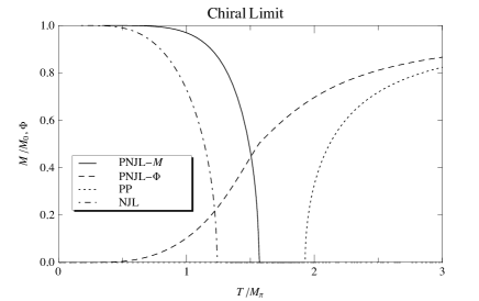
Figure 1: Normalized constituent quark mass and Polyakov loop in the chiral limit as a function of $T/M_{\pi}$, where $M_{\pi}=140$ MeV is the pion mass for $N_{c}=3$. See main text for details.

In Fig. 2, we show the chiral condensate $\langle\bar{\psi}\psi\rangle_{B}$ normalized to the chiral condensate in the vacuum $\langle\bar{\psi}\psi\rangle_{0}$ as a function of $|qB|$ in the chiral limit and at the physical point in the vacuum i.e. $T=\mu_{B}=0$ in the PNJL model. Note that here and in the following $|qB|$ is measured in units of the pion mass for $N_{c}=3$, i. e. $M_{\pi}=140$ MeV. Since the effects of the Polyakov vanish in the vacuum this is also the prediction of the NJL model. $\langle\bar{\psi}\psi\rangle_{B}$ is a monotonically increasing function of $|qB|$ and the system exhibits magnetic catalysis. In the NJL model and in the PNJL model at zero temperature, it is known that the chiral condensate grows quadritically with the field for small $|qB|$ in the chiral limit klevansky ; ebert22 . This is in contrast to chiral perturbation theory where the dependence is linear. In Ref. poli1 the authors investigate the chiral condensate as a function of the magnetic field $B$ for $SU(2)$ gauge theory using lattice simulations in the quenched approximation. The authors found that the linear behavior found in chiral perturbation theory can be described qualitatively by the function $\Sigma(B)=\Sigma_{0}\left(1+{{|qB|\over\Lambda_{B}^{2}}}\right)$, where $\Sigma_{0}$ and $\Lambda_{B}$ are fitting parameters. The parameters depend on the lattice parameters and we are using the value $\Lambda_{B}=1.53$ GeV, which corresponds to their largest lattice and their smallest lattice spacing $a$. The result is shown as the long-dashed line in Fig. 2 and is seen to agree reasonably well for magnetic field up to $|qB|\approx 6M_{\pi}^{2}$

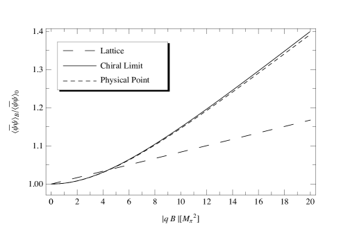
Figure 2: The chiral condensate $\langle\bar{\psi}\psi\rangle_{B}$ normalized to the chiral condensate in the vacuum $\langle\bar{\psi}\psi\rangle_{0}$ as a function of magnetic field $|qB|$ in the chiral limit (solid line) and at the physical point (dashed line) at zero temperature. Here $M_{\pi}=140$ MeV is the pion mass for $N_{c}=3$. Lattice results for pure-glue $SU(2)$ from Ref. poli1 is shown for comparison (long-dashed line).

We next consider the magnetic moment for a fermion of flavor $f$. In terms of the spin operator $\Sigma^{\mu\nu}={1\over 2i}(\gamma^{\mu}\gamma^{\nu}-\gamma^{\nu}\gamma^{\mu})$, it is defined by $\langle\bar{\psi}_{f}\Sigma^{\mu\nu}\psi_{f}\rangle$. In the case of constant magnetic field in the $z$-direction, only $\Sigma_{f}\equiv\Sigma^{12}$ is nonzero frasca . Using the properties of the $\gamma$-matrices, it can be shown that only the lowest Landau level (LLL) contributes to the expectation value of $\Sigma_{f}$ and reads

$$\langle\bar{\psi}_{f}\Sigma_{f}\psi_{f}\rangle_{B} = \langle\bar{\psi}_{f}\psi_{f}\rangle^{\rm LLL}_{B}\;,$$ (28)

where the superscript indicates that we include only the lowest Landau level. We then define the polarization by

$$\mu_{f} = {\langle\bar{\psi}_{f}\Sigma_{f}\psi_{f}\rangle_{B}\over\langle\bar{\psi}_{f}\psi_{f}\rangle_{B}}$$ (29)

$$= 1-{\langle\bar{\psi}_{f}\psi_{f}\rangle^{\rm HLL}_{B}\over\langle\bar{\psi}_{f}\psi_{f}\rangle_{B}}\;,$$

where the superscript $\rm HLL$ indicates that we have include only the higher Landau levels. In Fig. 3, we show the polarization $\mu={1\over 2}(\mu_{u}+\mu_{d})$ at $T=0$ and in the chiral limit as a function of $|qB|$. As expected, the polarization saturates for large magnetic fields to $\mu^{\infty}=1$. In this limit, the fermions in the higher Landau levels effectively become very heavy (cf. Eq. (15)), they decouple and the LLL dominates the physics. In this limit all the fermions are in the LLL and their spin is pointing in the same direction. The ratio of the mass of the fermions in the LLL and those in the HLL is essentially given by the dimensionless ratio $M^{2}/|qB|$. This ratio changes where the curve is steep and levels off for large values of $|qB|$.

Figure 3: The polarization $\mu$ as a function of $|qB|$ in the chiral limit and at zero temperature. Here $M_{\pi}=140$ MeV is the pion mass for $N_{c}=3$.

In Fig. 4, we show the critical temperature for the chiral transition (solid line) and the critical temperature for the deconfinement transition (dashed line) as functions of the magnetic field in the chiral limit for the PNJL model. The band is defined by $0.4<\Phi<0.6$ and shows the transition region for the deconfinement transition. We also show the critical temperature in the NJL model for comparison. The parameter $b$ in Eq. (14) has been tuned such that the two transitions coincide for $B=0$. We note that there is a splitting between the two transitions and that $T_{c}$ for the deconfinement is always lower than $T_{c}$ for the chiral transition and that the gap increases as a function of $B$. Thus, there should be a phase in which matter is deconfined and chiral symmetry is broken. The splitting was also observed in Ref. gatto1 ; fuku ; gatto2 ; mizher2 ; inverse2 ; calle , where the authors coupled the Polyakov loop to linear sigma model with quarks with $N_{c}=3$ colors. We first note that $T_{c}$ is decreasing ever so slightly from $|qB|=0$ to $|qB|\approx M_{\pi}^{2}$ and then increasing again. This is in contrast to the NJL model where $T_{c}$ is monotonically increasing as a function of $|qB|$. We discuss this further below.

Moreover, while $T_{c}$ for the chiral transition increases by more than 20% from $B=0$ to $|qB|=20M_{\pi}^{2}$, $T_{d}$ for the deconfinement transition is hardly affected. The width of the band is approximately 30 MeV. In contrast, the lattice simulations for $N_{c}=2$ reported in Ref. peter indicate that the critical temperature for deconfinement coincide with that of the chiral transition. Finally, we note that the determination of $a$ and $b$ has changed the critical temperature for the chiral transition dramatically. The increase of $T_{c}$ at $B=0$ is approximately $35$ MeV and is fairly constant up to $|qB|=20$ MeV. In order to compare the chiral transition at finite magnetic field in the NJL and PNJL model, i. e. the effects of the Polyakov loop, there might be other ways of determining $a$ and $b$. For example, one could force the deconfinement transition and the chiral transition in the PNJL model to take place at the same temperature for $B=0$ and force it to coincide with the chiral transition in the NJL model as well. This way of determining the parameters in $\Omega_{\rm gauge}$ would not require the input from lattice simulations.

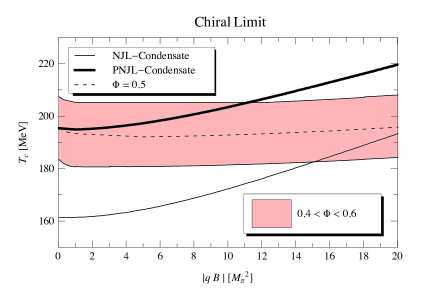
Figure 4: Critical temperature for the chiral transition (solid line) and critical temperature for the deconfinement transition (dashed line) as functions of magnetic field $|qB|$ in the chiral limit for the PNJL model. The band is defined by $0.4<\Phi<0.6$. We also show the critical temperature for the chiral transition (thin line) in the NJL model. Here $M_{\pi}=140$ MeV is the pion mass for $N_{c}=3$.

In Fig. 5, we show the thermodynamic potential $\Omega-\Omega_{0}$ divided by $F_{\pi}^{4}$ in the chiral limit for four different temperatures and $|qB|=20M_{\pi}^{2}$. For each temperature, we also give the value of the Polyakov loop. The critical temperature for the chiral transition is $T_{c}=220$ MeV and from the long-dashed line we see that transition is second order. Since the value of the Polyakov loop for $T=220$ MeV is $\Phi=0.68$, we conclude that the deconfinement transition has already taken place.

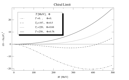
Figure 5: Thermodynamic potential $\Omega-\Omega_{0}$ divided by $F_{\pi}^{4}$ as a function of $M$ in the chiral limit for four different temperatures and $|qB|=20M^{2}_{\pi}$. Here $M_{\pi}=140$ MeV and $F_{\pi}=93$ MeV are the values for the pion mass and the pion decay constant for $N_{c}=3$. See main text for details.

In Fig. 6, we show the thermodynamic potential $\Omega-\Omega_{0}$ divided by $F_{\pi}^{4}$ as a function of $\Phi$ in the chiral limit for four different temperatures and $|qB|=20M^{2}_{\pi}$. For each temperature, we also give the value of the chiral condensate $M$. At $T=197$ MeV, we find that the minimum of the effective potential occurs for $\Phi={1\over 2}$ which defines the critical temperature for the deconfinement transition in the chiral limit. At this temperature, $M=286.2$ MeV and so we are still in the chirally broken phase. For $T=250$ MeV, the chiral condensate is vanishing and so we are in the chirally symmetric deconfined phase. In the chiral limit, the chiral transition is always second order.

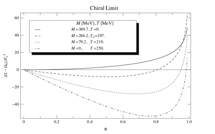
Figure 6: Thermodynamic potential $\Omega-\Omega_{0}$ divided by $F_{\pi}^{4}$ as a function of $\Phi$ in the chiral limit for four different temperatures and $|qB|=20M^{2}_{\pi}$. Here $M_{\pi}=140$ MeV and $F_{\pi}=93$ MeV are the values for the pion mass and the pion decay constant for $N_{c}=3$. See main text for details.

At the physical point, the chiral transition is a crossover and there is no well-defined critical temperature $T_{c}$ at which the chiral condensate vanishes. However, one can define a pseudo-critical temperature by the inflection point of the chiral condensate as a function of temperature. One can also define the transition region by the temperature range where $M$ varies between $0.4$ and $0.6$. This range depends on the magnetic field and gives rise to a band in the $B$–$T$ plane. This is shown as the dark band in Fig. 7. In the same manner, we define the crossover transition for the deconfinement transition by the the temperature range where $0.4<\Phi<0.6$. This is shown as the light band in Fig. 7. Moreover, as a guide to the eye, we also show the lines where $M/M_{0}={1\over 2}$ and $\Phi={1\over 2}$, respectively. For comparison, we also show the pseudocritical temperature for the chiral transition in the NJL model (dashed line). The curves indicate that the two transitions coincide for magnetic fields up to $|qB|\approx 5M_{\pi}^{2}$ and after that they split. The deconfinement transition is always taking place first. We notice that $T_{c}$ for the chiral transition first decreases as a function of $|qB|$ until $|qB|\approx 3M_{\pi}^{2}$ and then it starts to increase again. At the physical point where there is only a cross-over, the width of the transition is much bigger than this decrease in $T_{c}$. The difference between $T_{c}(|qB|=0)$ and $T_{c}(|qB|=3M_{\pi}^{2})$ is only a few MeV which is comparable to the drop found by Bali et al. budaleik ; gunnar for $N_{c}=3$. However, note that these authors find that $T_{c}$ is decreasing as a function in the entire region they investigated, namely magnetic fields up to $|qB|\approx$ 1 (GeV)², and that the drop in $T_{c}$ is approximately 20 MeV in this range. The non-monotomic behavior of $T_{c}$ as a function of $|qB|$ in the PNJL model is absent in the NJL model and we attribute this to the coupling to the Polyakov loop. Another possible explanation for the non-monotonic behaviour is that it could be very well an artifact of our mean field approximation. Finally, we note that the band of the chiral transition is much narrower than that of the deconfinement transition (approximately $T=10$ MeV versus approximately $T=30$ MeV) and is so significantly faster.

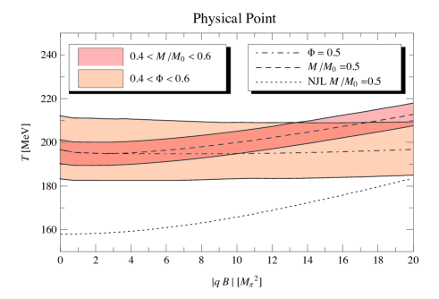
Figure 7: Transition region at the physical point as a function of $|qB|$. Here $M_{\pi}=140$ MeV is the value for the pion mass for $N_{c}=3$. For comparison, the dashed line shows the pseudocritical temperature in the NJL model. See main text for details.

In Fig. 8, we show the normalized thermodynamic potential $\Omega/F_{\pi}^{4}$ as a function of $M$ and $\Phi$ in the chiral limit with $|qB|=20M_{\pi}^{2}$ for different temperatures. From left to right $T=100$ MeV, $T=200$ MeV, $T=219$ MeV, and $T=250$ MeV. For $T=100$ MeV, we are in the confined and the chirally broken phase, while for $T=200$ MeV, the value of $\Phi$ is slightly above ${1\over 2}$ ($\Phi={1\over 2}$ for $T=197$ MeV). The minimum is still for nonzero $M$ and so chiral symmetry is broken. For $T=219$ MeV, $M/M_{0}$ is still nonozero ($T_{c}=220$ MeV) and so we are just below the chiral transition.

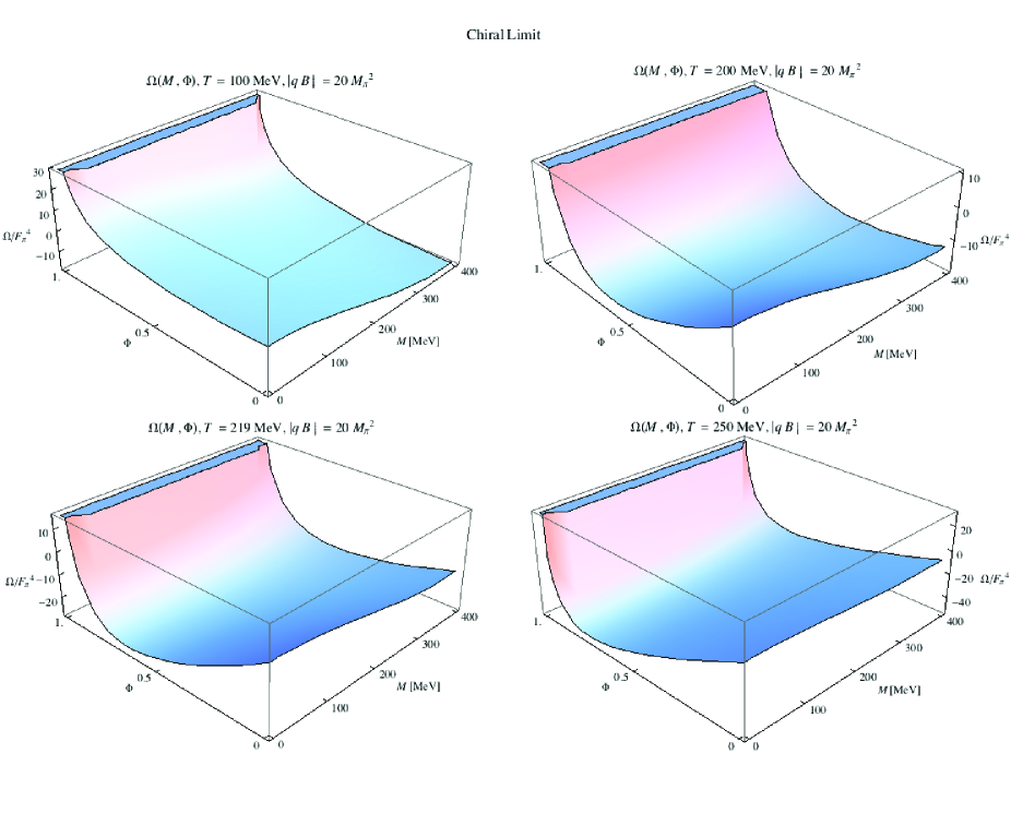
Figure 8: The normalized thermodynamic potential $(\Omega-\Omega_{0})/F_{\pi}^{4}$ in the chiral limit as a function of $M$ and $\Phi$ for four different temperatures and $|qB|=20M_{\pi}$. From left to right $T=100$ MeV, $T=200$, Mev, $T=219$ MeV, and $T=250$ MeV. Here $M_{\pi}=140$ MeV and $F_{\pi}=93$ MeV are the values for the pion mass and the pion decay constant for $N_{c}=3$. See main text for details.

IV Concluding remarks

In the present paper, we have considered two-color two-flavor QCD in a constant magnetic background using the PNJL model. In the chiral limit, the chiral transition is always second order with mean-field critical exponents. The order of the transition is in agreement with universality arguments. Our results for the chiral transition as a function of $|qB|$ shows some interesting behavior: the critical temperature first decreases and then it increases. This behavior is more pronounced at the physical point (cf. Figs. 4 and 7). In this case the transition temperature decreases for values of $|qB|$ up to approximately 3$M_{\pi}^{2}$ and then it increases. We therefore have inverse magnetic catalysis in this range of $|qB|$ and results from the coupling to the Polyakov loop since the transition temperature is increasing for all values of $|qB|$ in the NJL model. Even though we attribute the coupling to the Polyakov loop as the mechanism responsible for the inverse catalysis in the range mentioned, there is the possibility that this effect is actually an artifact of the mean-field approximation we use in our calculations and it would not survive if we used more advanced techniques. For example it is known that critical points in the $\mu-T$ plane in some low-energy effective theories display a critical endpoint in mean-field calculations. If one uses functional renormalization techniques, they disappear strod . Thus, it is worthwhile pursuing this behaviour using more sophisticated methods before we conclude more firmly about the nature of this effect. The lattice simulations of Ref. peter seem to indicate a transition temperature which is increasing with the strength of the magnetic field. However, one must be cautious since they did not take the continuum limit and used $N_{f}=4$ with identical electric charges. A careful study using 1+1 flavors, $N_{c}=2$, and taking the continuum limit is necessary to compare with the results in the present paper.

We next turn to the case $N_{c}=3$. The inverse catalysis for temperature around $T_{c}$ seen in budaleik ; gunnar ; falk ; gunnar2 hinges on taking continuum limit and using physical quark masses. For larger unphysical quark masses, the system shows catalysis at finite temperatures. Given the lattice results for $N_{c}=3$ it is clear that all the model calculations to date fail at temperatures $T$ around $T_{c}$ and in particular does not incorporate that magnetic catalysis is turned into inverse magnetic catalysis around the transition. This is independent of whether it is a mean-field calculation or one goes beyond using e.g. functional renormalization group techniques skokov1 ; anders . In the recent papers falk ; gunnar2 , the authors provide a plausible explanation for the discrepancy between the model calculations and the lattice simulations. The chiral condensate can be written as

$$\langle\bar{\psi}\psi\rangle = {1\over{\cal Z}(B)}\int d{\cal U}e^{-S_{g}}\det(D\!\!\!\!/(B)+m){\rm Tr}(D\!\!\!\!/(B)+m)^{-1}\;,$$ (30)

where the partition function is

$${\cal Z}(B) = \int d{\cal U}e^{-S_{g}}\det(D\!\!\!\!/(B)+m)\;,$$ (31)

and $S_{g}$ is the pure-glue action. Thus there are two contributions to the chiral condensate, namely the operator itself (coined valence contribution) and the change of typical gauge configurations sampled, coming from the determinant in Eq. (30) (coined sea contribution). At least for small magnetic fields one can disentangle these contributions by defining

$$\langle\bar{\psi}\psi\rangle^{\rm val} = {1\over{\cal Z}(0)}\int d{\cal U}e^{-S_{g}}\det(D\!\!\!\!/(0)+m){\rm Tr}(D\!\!\!\!/(B)+m)^{-1}\;,$$ (32)

$$\langle\bar{\psi}\psi\rangle^{\rm sea} = {1\over{\cal Z}(B)}\int d{\cal U}e^{-S_{g}}\det(D\!\!\!\!/(B)+m){\rm Tr}(D\!\!\!\!/(0)+m)^{-1}\;.$$ (33)

At zero temperature, both contributions are positive leading to magnetic catalysis. At temperatures around the transitions temperature, the valence condensate is still positive while the sea condensate is negative. Hence there is a competition between the two leading to a net inverse catalysis. The sea contribution can be viewed as a back reaction of the fermions on the gauge fields and this effect is not present in the model calculations as there are no dynamical gauge fields. If such a back reaction can be mimicked or incorporated in the model calculations, one may be able to obtain agreement with the lattice simulations.

It is also interesting to note that the magnetic field hardly affects the critical temperature for deconfinement. This is in line with the observation of mizher . Morever, our results seem to indicate that the two transitions coincide at the physical point up to fairly large values of the magnetic field. $|qB|\approx 5M_{\pi}^{2}$.

Finally, we would like to comment on the role of quantum fluctuations and related renormalization issues. In a one-loop calculation of the effective potential it is possible to separate the vacuum contributions from the thermal contributions. In some case, it therefore makes sense to investigate the role of the vacuum fluctuations. For example, in the QM, it is customary to treat the bosons at tree level and the fermions at the one-loop level. In this case it was shown in Ref. skokov for $B=0$ that the order of the phase transition depends whether the zero-temperature fluctuations are included or not; if they are, the chiral transition is second order and if they are not, it is first order. The same effect of the vacuum fluctuations were found in the entire $\mu_{B}$–$T$ plane in strong magnetic fields in rashid . In contrast to the QM model with quarks, this question does not make sense in the (P)NJL model. The reason is that chiral symmetry breaking in the (P)NJL is always a loop effect in contrast to the QM model where it is built into the tree-level potential. In a similar manner, Ref. boomsma finds that a crossover transition (for $N_{c}=3$) at the physical point remains a crossover at finite magnetic field $B$ in an NJL model calculation. This is in contrast to Ref. mizher where it is found that strong magnetic fields turn the crossover into a first-order transition. In their work, the authors use the QM model and renormalize by subtracting the fermionic vacuum fluctuations at $B=0$.

References

- (1) Lect. Notes Phys. ”Strongly interacting matter in magnetic fields” (Springer), edited by D. Kharzeev, K. Landsteiner, A. Schmitt, and H.-U. Yee.
- (2) R. C. Duncan and C. Thompson, Astrophys. J. 392 L9 (1992).
- (3) V. Skokov, A. Y. Illarionov, and V. Toneev, Int. J. Mod.Phys. A 24 5025, (2009).
- (4) A. Bzdak and V. Skokov, Phys.Lett. B 710, 171 (2012).
- (5) D. E. Kharzeev, L. D. McLerran, and H. J. Warringa, Nucl. Phys. A 803, 227 (2008).
- (6) T. Vachaspati, Phys. Lett. B 265, 258 (1991).
- (7) K. Enqvist and P. Olesen, Phys. Lett. B 319, 178 (1993).
- (8) M. Laine K. Kajantie, M. Laine, J. Peisa, K. Rummukainen, M. E. Shaposhnikov, Nucl. Phys. B 544, 357 (1999).
- (9) A. De Simone, G. Nardini, M. Quiros, and A. Riotto, JCAP 1110, 030 (2011).
- (10) S. P. Klevansky and R. H. Lemmer, Phys. Rev. D 39, 3478, (1989).
- (11) K.G. Klimenko, Z. Phys. C 54, 323 (1992).
- (12) V. P. Gusynin, V. A. Miransky, and I. A. Shovkovy, Phys. Rev. Lett. 73, 3499 (1994).
- (13) V. P. Gusynin, V.A. Miransky, and I. A. Shovkovy, Nucl. Phys. B 462, 249 (1996).
- (14) D. Ebert, K. G. Klimenko, M. A. Vdovichenko, and A. S. Vshivtsev, Phys. Rev. D 61 025005 (1999).
- (15) I. Shushpanov and A. V. Smilga, Phys. Lett. B 402 351, (1997).
- (16) T. D. Cohen, D. A. McGady, and E. S. Werbos, Phys. Rev. C 76, 055201 (2007).
- (17) K. Fukushima and J. M. Pawlowski, Phys. Rev. D 86, 076013 (2012).
- (18) K. Fukushima and Y. Hidaka, Phys. Rev. Lett., 110, 031601 (2013).
- (19) V. V. Braguta, P. V. Buividovich, T. Kalaydzhyan, S. V. Kuznetsov, and M. I. Polikarpov, PoS LATTICE2010, 190 (2010), Phys. Atom. Nucl. 75, 488 (2012).
- (20) G. S. Bali, F. Bruckmann, G. Endrődi, Z. Fodor, S. D. Katz, S. Krieg, A. Schafer, and K. K. Szabo, JHEP 1202, 044 (2012).
- (21) G. S. Bali, F. Bruckmann, G. Endrődi, Z. Fodor, S.D. Katz, and A. Schafer, Phys. Rev. D 86, 071502 (2012)
- (22) R. Gatto and M. Ruggieri, Phys. Rev. D 82, 054027 (2010).
- (23) D. C. Duarte, R. L. S. Farias, and R. O. Ramos, Phys. Rev. D 84, 083525 (2011).
- (24) N. O. Agasian, Phys. Lett. B 488, 39 (2000).
- (25) J. O. Andersen, Phys. Rev. D 86, 025020 (2012); JHEP 1210, 005 (2012).
- (26) N. O. Agasian and S. M. Fedorov, Phys. Lett. B 663, 445 (2008).
- (27) S. S. Avancini, D. P. Menezes, M. B. Pinto, and C. Providencia, Phys.Rev. D 85 091901 (2012).
- (28) G. N. Ferrari, A. F. Garcia, and M. B. Pinto, Phys. Rev. D 86, 096005 (2012).
- (29) K. Fukushima, M. Ruggieri, and R. Gatto, Phys. Rev. D 81, 114031 (2010).
- (30) E. S. Fraga and A. J. Mizher, Phys. Rev. D. 78, 025016 (2008).
- (31) V. Skokov, Phys. Rev. D 85, 03426 (2012).
- (32) J. O. Andersen and A. Tranberg, JHEP 1208, 002 (2012).
- (33) J. O. Andersen and R. Khan, Phys. Rev. D 85, 065026 (2012).
- (34) M. Ferreira, P. Costa, D. P. Menezes, C. Providencia, N. Scoccola, arXiv:1305.4751v1 [hep-ph].
- (35) R. Gatto and M. Ruggieri, Phys. Rev. D 83, 034016 (2011).
- (36) E. S. Fraga and L. F. Palhares, Phys. Rev. D 86, 016008 (2012).
- (37) A. J. Mizher, M. N. Chernodub and E. S. Fraga, Phys. Rev. D 82, 105016 (2010).
- (38) E. S. Fraga, J. Noronha, and L. F. Palhares, Phys. Rev. D 87, 114014 (2013).
- (39) M. D’Elia, S. Mukherjee, and F. Sanfilippo, Phys. Rev. D 82, 051501 R (2010).
- (40) M. D’Elia and F. Negro, Phys. Rev. D 83, 114028 (2011).
- (41) T. Inagaki, D. Kimura, and T. Murata, Prog. Theor. Phys. 111, 371 (2004).
- (42) F. Preis, Anton Rebhan, and Andreas Schmitt. JHEP 1103, 033 (2011).
- (43) G. S. Bali, F. Bruckmann, G. Endrodi, F. Gruber, and A. Schaefer JHEP 1304 130 (2013).
- (44) F. Bruckmann, G. Endrodi, and T. G. Kovacs, JHEP 1304, 112 (2013).
- (45) L. A. Kondratyuk and M. M. Gianinni, Phys. Lett. B 269 139 (1991).
- (46) J. B. Kogut, M. A. Stephanov, and D. Toublan, Phys. Lett. B 464, 183 (1999).
- (47) K. Splittorff, D.T. Son, and M. A. Stephanov, Phys. Rev. D 64, 016003 (2001).
- (48) C. Ratti and W. Weise, Phys. Rev. D 70, 054013 (2004).
- (49) P. Cea, L. Cosmai, M. D’Elia, and A. Papa JHEP 0702, 066 (2007.)
- (50) S. Hands, S. Kim, J-I. Skullerud, Phys. Rev. D 81 091502 (2010).
- (51) T. Kanazawa, Tilo Wettig, N. Yamamoto, JHEP 0908, 003 (2009).
- (52) T. Brauner, K. Fukushima, and Y. Hidaka Phys. Rev. D 80, 074035 (2009); Erratum-ibid. D 81, 119904 (2010).
- (53) J. O. Andersen and T. Brauner, Phys. Rev. D 81, 096004 (2010).
- (54) T. Zhang, T. Brauner, A. Kurkela, A. Vuorinen, JHEP 1202, 139 (2012).
- (55) N. Strodthoff, B.-J. Schaefer, L. von Smekal, Phys. Rev. D 85, 074007 (2012).
- (56) K. Kashiwa, T. Sasaki, and H. Kounu, Phys. Rev. D 87 016015 (2013).
- (57) S. Imai, H. Toki, and W. Weise e-Print: arXiv:1210.1307 [nucl-th].
- (58) P. V. Buividovich, M. N. Chernodub, E. V. Luschevskaya, and M. I. Polikarpov, Phys. Lett. B 682, 484 (2010).
- (59) P. V. Buividovich, M. N. Chernodub, E. V. Luschevskaya, and M. I. Polikarpov, Nucl. Phys. B 826, 313 (2010).
- (60) E.-M. Ilgenfritz, M. Kalinowski, M. Müller-Preussker, B. Petersson, and A. Schreiber, Phys. Rev. D 85, 114504 (2012).
- (61) B. Svetitsky and L. G. Yaffe, Nucl. Phys. B 210, 423 (1982).
- (62) K. Fukushima, Phys. Lett. B 591, 277 (2004).
- (63) E. Megias, E. Ruiz Arriola, and L.L. Salcedo, Phys. Rev. D 74, (2006) 065005; ibid 74, 114014 (2006).
- (64) G.-F. Sun, L. He, P. Zhuang, Phys. Rev. D 75, 096004 (2007).
- (65) C. Sasaki, B. Friman, and K. Redlich, Phys. Rev. D 75, 074013 (2007).
- (66) B. Lucini, A. Rago, and E. Rinaldi, Phys. Lett. B 712 279 (2012).
- (67) K. Fukushima, Phys. Rev. D 77, 114028 (2008).
- (68) M. Frasca and M. Ruggieri, Phys. Rev. D 83, 094024 (2011).
- (69) N. Callebaut, D. Dudal, and H. Verschelde, PoS FACESQCD 046 (2010).
- (70) V. Skokov, B. Friman, E. Nakano, K. Redlich, and B.-J. Schaefer, Phys.Rev. D 82, 034029 (2010).
- (71) J. K. Boomsma and D. Boer, Phys. Rev. D 81, 074005 (2010).