Manipulating energy and spin currents in nonequilibrium systems of interacting qubits

Abstract

We consider generic interacting chain of qubits, which are coupled at the edges to baths of fixed polarizations. We can determine the nonequilibrium steady states, described by the fixed point of the Lindblad Master Equation. Under rather general assumptions about local pumping and interactions, symmetries of the reduced density matrix are revealed. The symmetries drastically restrict the form of the steady density matrices in such a way that an exponentially large subset of one–point and many–point correlation functions are found to vanish. As an example we show how in a Heisenberg spin chain a suitable choice of the baths can completely switch off either the spin or the energy current, or both of them, despite the presence of large boundary gradients.

I Introduction

The impressive progress in experimental manipulation of nanowires and quantum dots makes it possible to investigate quantum systems consisting of a few quantum dots or quantum bits. On the other hand, manipulations/operations on a single quantum bit (e.g., application of a quantum gate) are at the basis of the functioning of any elementary block of a quantum computing device. However, a theoretical understanding of microscopic quantum systems out of equilibrium (e.g. under constant pumping or continuous measurement by a quantum probe) is far from being complete, apart from simple cases like a single two-level system or a quantum harmonic oscillator under external pumping or in contact with reservoirs Petruccione ; PlenioJumps . On the other hand, using the dissipative dynamics for the preparation of quantum states with required properties is becoming a promising field of research ZollerNature2008 ; ZollerPRA . In this respect, the role of sufficiently simple spatially extended systems, amenable to both analytic and numerical investigations, becomes important.

Unlike a quantum system evolving coherently, whose evolution at any time depends on the initial state, a quantum system with pumping tends to a steady state, independently of the initial conditions. This allows to manipulate the steady state of the system by a suitable choice of the pumping. In this paper we first illustrate how to accomplish such a task for a general system of interacting quantum spins. In particular we consider symmetries of the density matrix that impose rigid constraints on the properties of the nonequilibrium steady state, thus entailing, for instance, exact vanishing of cumulative correlation functions, like certain components of the structure factor. Then, we specialize our analysis to the one dimensional driven XXZ chain of quantum spins in the presence of pumping applied at the edges. We show that, for particular realizations of the pumping and irrespectively of the system size, one can switch on and off the spin and/or the heat currents in the nonequilibrium steady-state. Such an approach unveils new interesting perspectives in the study of driven spin chain models. They have been mainly investigated to understand under which conditions the spin and the energy currents in the steady state exhibit anomalous or ballistic behavior reviewBrenig07 ; zotos ; KlumperLectNotes2004 . In this regard, we want to point out that the results presented in this paper hold independently of the anomalous or ballistic features of transport ZotosBallistic97 and even in the absence of integrability.

In Section II we present the general model of Lindblad master equation and discuss how symmetries may affect its properties. Specific forms of Lindblad operators acting on quantum spin models are introduced in Section III. In particular, we devote special attention to parity selection rules in Section IV. Section V deals with the special case of the Lindblad dynamics for the one dimensional XXZ model of qubits. It has been chosen to illustrate in detail how our findings apply to a simple model, that has been the object of intense resent research. Specifically, in subsection V.1 we discuss the kind of symmetries emerging in this model for Lindblad operators of target type, while subsection V.2 is devoted to the analysis of spin and energy conductance in the presence of gradients. Conclusions and perspectives are contained in Section VI.

II Lindblad Master Equation and its symmetries

We consider the quantum Master equation in the Lindblad form Petruccione ; Wichterich07 ,

$$\frac{\partial\rho}{\partial t}=i\left[\rho,H\right]-\frac{1}{2}\sum_{m}\left\{\rho,L_{m}^{(p)\dagger}L_{m}^{(p)}\right\}+\sum_{m,p}L_{m}^{(p)}\rho L_{m}^{(p)\dagger},$$ (1)

where we have set $\hbar=1$; $\rho$ is the reduced density matrix, $H$ is the Hamiltonian of the system and $L_{m}^{(p)}$ is the Lindblad operator. It is easy to verify that $\frac{\partial}{\partial t}Tr(\rho)=0,\rho^{+}=\rho,\frac{\partial}{\partial t}Tr(\rho^{2})\neq 0$. The first two relations are necessary for interpreting $\rho$ as a density matrix, with $Tr(\rho)=1$, while the latter implies that we deal with an open system: an initially pure state $\rho=|\phi\rangle\langle\phi|$ will not remain pure in the course of time. The Lindblad equation is the most general Markovian equation of motion for the reduced density matrix, conserving positivity and trace, and having a semigroup property Petruccione .

The non-unitary part of the Lindblad Master equation (LME) makes the dynamics irreversible. In the course of time, any initial state will relax to a nonequilibrium steady state (NESS), described by the time-independent solution of the Master equation. Our purpose is to reveal symmetries of the LME and respective constraints on the NESS, which the symmetries impose. In the simplest case, the constraints on NESS take the form of selection rules, according to which a subset of the matrix elements of the reduced density matrix has to vanish.

Let us denote the right-hand side of LME as $\mathcal{L}[\rho]$.   If it is invariant under a unitary transformation $U$, i.e. $\mathcal{L}[U\rho U^{\dagger}]=U\mathcal{L}[\rho]U^{\dagger}$, it follows that $\tilde{\rho}(t)=U\rho(t)U^{\dagger}$ is a new solution of LME. In general the solutions $\tilde{\rho}(t)$ and $\rho(t)$ describe different time evolutions. If the nonequilibrium steady state (NESS) of the system $\rho_{NESS}=\lim_{t\rightarrow\infty}\rho(t)$ is unique EvansUniqueness , then the trajectories $\rho(t)$ and $\tilde{\rho}(t)$ eventually converge in time to the same asymptotic solution, $\lim_{t\rightarrow\infty}\rho(t)=\lim_{t\rightarrow\infty}\tilde{\rho}(t)=\rho_{NESS}$. Accordingly, the unique steady state of the system has to be invariant under the transformation $U$,

$$\rho_{NESS}=U\rho_{NESS}U^{\dagger}.$$ (2)

This implies also that the expectation value of any physical observable of interest $\hat{f}$, measured in the steady state, $\langle\hat{f}\rangle\equiv Tr\left(\hat{f}\rho_{NESS}\right)$, has to satisfy the relations

$$\langle\hat{f}\rangle=Tr\left(\hat{f}U\rho_{NESS}U^{\dagger}\right)=\langle U^{\dagger}\hat{f}U\rangle.$$ (3)

.In particular, if $\hat{f}$ changes sign under the action of $U$,

$$U^{\dagger}\hat{f}U=-\hat{f},$$ (4)

it follows that

$$\langle\hat{f}\rangle =Tr\left(U^{\dagger}\hat{f}U\rho_{NESS}\right)$$

$$=-Tr\left(\hat{f}\rho_{NESS}\right)=-\langle\hat{f}\rangle\,\,\rightarrow\,\,\langle\hat{f}\rangle=0\,\,.$$ (5)

On the contrary, if $\hat{f}$ is invariant under the action of $U$, i.e.

$$U^{\dagger}\hat{f}U=\hat{f}\,\,,$$ (6)

no consequences for $\langle\hat{f}\rangle$ can be drawn,

$$\langle\hat{f}\rangle=Tr\left(U^{\dagger}\hat{f}U\rho_{NESS}\right)=Tr\left(\hat{f}\rho_{NESS}\right)\,\,.$$ (7)

For instance, let us suppose that a two-level open quantum system, described by a generic density matrix $\rho=\frac{1}{2}I+\frac{1}{2}\sum_{\alpha}\langle\sigma^{\alpha}\rangle\sigma^{\alpha}$ ($\sigma^{\alpha}$ being Pauli matrices), is invariant under the transformation $U=\sigma^{z}$, and has a unique steady state. Since $\sigma^{z}\sigma^{x}\sigma^{z}=-\sigma^{x}$, $\sigma^{z}\sigma^{y}\sigma^{z}=-\sigma^{y}$ and $\sigma^{z}\sigma^{z}\sigma^{z}=\sigma^{z}$, from (4) we can conclude that $\langle\sigma^{x}\rangle=\langle\sigma^{y}\rangle=0$, while $\langle\sigma^{z}\rangle$ is invariant under the action of $U$.

III Lindblad operators

Here we focus on the most commonly used types of Lindblad operators: (i) those targeting a given value of observables $\langle\sigma_{p}^{\alpha}\rangle$; (ii) those responsible for dephasing, or decoherence, whose action favors the evolution to a classical state; (iii) the non-local variants of the previous cases.

Lindblad operators targeting a given value of $z-$ spin projection $\sigma_{\text{target}}^{z}$ at a chosen site $p$ have the form of creation-annihilation operators,

$$L_{1}^{(p)} =\alpha(\sigma_{p}^{x}+i\sigma_{p}^{y})=\alpha\sigma_{p}^{+}$$ (8)

$$L_{2}^{(p)} =\beta(\sigma_{p}^{x}-i\sigma_{p}^{y})=\beta\sigma_{p}^{-}.$$ (9)

The equations of motion for the expectation values of the operators $\sigma_{p}^{x},\sigma_{p}^{y},\sigma_{p}^{z}$  read

$$\frac{d\langle\sigma_{p}^{z}\rangle}{dt} ={\mathcal{H}}(\sigma_{p}^{z})-\Gamma_{z}(\langle\sigma_{p}^{z}\rangle-\sigma_{\text{target}}^{z})$$ (10)

$$\frac{d\langle\sigma_{p}^{x}\rangle}{dt} ={\mathcal{H}}(\sigma_{p}^{x})-\Gamma_{x}\langle\sigma_{p}^{x}\rangle$$

$$\frac{d\langle\sigma_{p}^{y}\rangle}{dt} ={\mathcal{H}}(\sigma_{p}^{y})-\Gamma_{y}\langle\sigma_{p}^{y}\rangle\,\,,$$

where we introduce the shorthand notation ${\mathcal{H}}(f_{p})\equiv-iTr\left(f_{p}\left[H,\rho\right]\right)$, and

$$\Gamma_{z} =4(\alpha^{2}+\beta^{2});\text{ \ }\sigma_{\text{target}}^{z}=\frac{\alpha^{2}-\beta^{2}}{\alpha^{2}+\beta^{2}}$$ (11)

$$\Gamma_{x} =\Gamma_{y}=\Gamma_{z}/2\,.$$ (12)

If the coupling constant $\Gamma_{z}$ is sufficiently large with respect to the norm of the Hamiltonian in equations (10), then ${\mathcal{H}}$ can be neglected and the averages $\langle\sigma_{p}^{i}(t)\rangle$ converge, after some relaxation time of order $1/\Gamma_{\eta},$ to their ”targeted” values $\sigma_{\text{target}}^{x}=0,\sigma_{\text{target}}^{y}=0,\sigma_{\text{target}}^{z}=\left(\alpha^{2}-\beta^{2}\right)/\left(\alpha^{2}+\beta^{2}\right)$ as follows

$$\langle\sigma_{p}^{\eta}(t)\rangle=\sigma_{\text{target}}^{\eta}+\langle\sigma_{p}^{\eta}(0)-\sigma_{\text{target}}^{\eta}\rangle e^{-\Gamma_{\eta}t}\,.$$ (13)

Lindblad operators of type (9) naturally appear in the problem of an atom interacting with a quantized radiation field GardinerZoller2000 , in spin chains coupled to a bath of fixed polarization, in electron paramagnetic resonance experiments and in studies of quantum transport Pros08 ; ZunkovichJStat2010ExactXY ; BenentiPRB2009 ; ProsenExact2011 ; JesenkoZnidaric2011 ; Casati2009 ; ProsenNY2010 ; Znidaric2011 ; ProsenZnidaric ; ZnidaricJStat2010 .

Lindblad operators targeting a given value of $x-$spin projection or $y-$spin projection are given by the appropriate cyclic rotation of the operators (9), i.e.

$$V_{1}=\alpha(\sigma_{p}^{y}+i\sigma_{p}^{z}),\text{ \ }V_{2}=\beta(\sigma_{p}^{y}-i\sigma_{p}^{z})\text{ }$$ (14)

with target $\sigma_{\text{target}}^{x}=\left(\alpha^{2}-\beta^{2}\right)/\left(\alpha^{2}+\beta^{2}\right)$ at site $p$ and

$$W_{1}=u(\sigma_{p}^{z}+i\sigma_{p}^{x}),\text{ \ }W_{2}=v(\sigma_{p}^{z}-i\sigma_{p}^{x})\text{ }$$ (15)

with target $\sigma_{\text{target}}^{y}=\left(u^{2}-v^{2}\right)/\left(u^{2}+v^{2}\right)$ at site $p$. The relaxation to the targeted values can be described in complete analogy with (11)-(13), see Lindblad2011 .

Dephasing Lindblad operators have the form

$$L_{deph}^{(p)}=\sqrt{\gamma_{p}}\sigma_{p}^{z}$$ (16)

and describe the presence of a dephasing noise in the dynamics, which causes decoherence (i.e., vanishing of non-diagonal density matrix elements) with rate $\gamma_{p}$ at site $p$. The local equations of motion, analogous to (10), have the simple form

$$\frac{d\langle\sigma_{p}^{x,y}\rangle}{dt}=-2\gamma_{p}\langle\sigma_{p}^{x,y}\rangle\,\,\,,\,\,\,\frac{d\langle\sigma_{p}^{z}\rangle}{dt}=0\,.$$ (17)

The coupling to a heat bath is often modelled by the application of the dephasing Lindblad operators (16) at all sites of the system.

Lindblad operators, acting on more than one site, introduce incoherent non-local processes. For instance the Lindblad operator

$$L_{hopp}^{(p,q)}=\sqrt{\gamma}\sigma_{p}^{+}\sigma_{q}^{-}$$ (18)

describes incoherent spin flips between sites $p$ and $q$ EislerBallistic .

IV Parity symmetry selection rules for Lindblad dynamics

We consider a generic open system of qubits, with internal pair interactions, described by the Lindblad Master equation (1), with the Hamiltonian

$$H =\sum_{k,m=1}^{N}J_{X}(k,m)\sigma_{k}^{x}\sigma_{m}^{x}+J_{Y}(k,m)\sigma_{k}^{y}\sigma_{m}^{y}$$ (19)

$$+J_{Z}(k,m)\sigma_{k}^{z}\sigma_{m}^{z}+\sum_{k=1}^{N}h_{k}\sigma_{k}^{z}\,\,,$$

where $J_{\alpha}(k,m)$ are couplings between qubits $k,m$, and $h_{k}$ are local magnetic fields. We do not impose any restriction on the space dimension or on the geometry, but we just assume the connectivity of the graph. The system can be subject to external pumping and/or external noise, modelled by the $z$-polarization targeting operators (9), dephasing Lindblad operators (16) and incoherent hoppings (18), with all of these operators acting on an arbitrary subset of sites. Then, if the steady state is unique, the transformation $\Omega_{z}=(\sigma^{z})^{\otimes_{N}}=\sigma^{z}\otimes\sigma^{z}\otimes...\otimes\sigma^{z}$ , $\Omega_{z}^{-1}=\Omega_{z}$ identifies a symmetry of the Master equation, thus yielding the relation

$$\rho_{NESS}=\Omega_{z}\rho_{NESS}\Omega_{z}.$$ (20)

Indeed, Hamiltonian (19) as well as dephasing Lindblad operators (16) and incoherent hoppings (18) are invariant under $\Omega_{z}$, while $z-$polarization targeting operators (9) change sign under its action. Since the Lindblad part of the evolution equation is quadratic in $L_{m}$, LME is invariant under $\Omega_{z}$. The symmetry (20) is known in spin models as parity symmetry (P–symmetry). In the special case where the total set of Lindblad operators contains either only dephasing Lindblad operators (16) or only z-polarization targeting Lindblad operators (9), LME has one further symmetry, the PT- symmetry, which has interesting consequences on the full spectrum of the Lindblad superoperator ProsenSymmetries . In our general setting, where the dephasing and the polarization targeting Lindblad operators are mixed, the quantum Lindblad dynamics is not PT-invariant. Another remark concerns our crucial assumption of a uniqueness of the steady state. The existence and uniqueness of the steady state is guaranteed by the completeness of the algebra, generated by the set of operators $\{H,L_{m},L_{m}^{\dagger}\}$ under multiplication and addition EvansUniqueness , and it is verified straightforwardly as in ProsenUniqueness , for any choice of a set of the Lindblad operators $\{L_{m}\}$, provided the set contains at least one polarization targeting operator (8) or (9).

The P–symmetry yields severe limitations on the nonequilibrium steady state $\rho_{NESS}$. We indicate with $\rho_{j_{1}j_{2}...j_{N}}^{i_{1}i_{2}...i_{N}}$ the matrix element of $\rho_{NESS}$ in the natural basis, labelled by indexes $i_{1},i_{2},...j_{N}$ which take values $-1,1$. Let us calculate how the matrix element $\rho_{j_{1}j_{2}...j_{N}}^{i_{1}i_{2}...i_{N}}$ changes under the action of the P–symmetry operator $\Omega_{z}$. One obtains

$$\left((\sigma^{z})^{\otimes_{N}}\rho(\sigma^{z})^{\otimes_{N}}\right)_{j_{1}j_{2}...j_{N}}^{i_{1}i_{2}...i_{N}}=\rho_{j_{1}j_{2}...j_{N}}^{i_{1}i_{2}...i_{N}}\times\prod\limits_{m=1}^{N}i_{m}j_{m}.$$ (21)

The factor $K=\prod\limits_{m=1}^{N}i_{m}j_{m}$ may only take values $1$ and $-1$. If $K=1$, the P–symmetry does not yield any constraint on $\rho$. Conversely, if $K=-1$, from (20) it follows that the corresponding matrix element vanishes,

$$\rho_{j_{1}j_{2}...j_{N}}^{i_{1}i_{2}...i_{N}}\equiv 0\,\,\,\,\,\text{ if }\,\,\,\,\,\prod\limits_{m=1}^{N}i_{m}j_{m}=-1\text{.}$$ (22)

We call this condition a parity selection rule (PSR). If (22) holds, simple analysis shows that each row and each column of $\rho$ contains $2^{N-1}$ zero entries. For instance, the first row of the density matrix for 3 sites $\rho_{\alpha\beta\gamma}^{111}$ contains four null elements: $\rho_{1\text{ }1\text{ }-1}^{1\text{ }1\text{ }1}=\rho_{-1\text{ }1\text{ }1}^{1\text{ }1\text{ }1}=\rho_{1\text{ }-1\text{ }1}^{1\text{ }1\text{ }1}=\rho_{-1\text{ }-1\text{ }-1}^{1\text{ }1\text{ }1}=0$. More generally, it can be easily realized that by a suitable reshuffling of rows/columns the $2^{N}\times 2^{N}$ density matrix satisfying (22) can be brought into a block-diagonal form, with two blocks of equal size $2^{N-1}\times 2^{N-1}$.

An important feature of PSR is that any subsystem made of $n$ qubits, described by the reduced density matrix $\rho_{(n)}=Tr_{N-n}\rho$, keeps the same symmetry, as it can be easily verified,

$$\rho_{(n)j_{1}j_{2}...j_{n}}^{\text{ \ \ \ \ }i_{1}i_{2}...i_{n}}\equiv 0\text{ for }\prod\limits_{m=1}^{n}i_{m}j_{m}=-1.$$ (23)

For $n=2$ the explicit form of the generic density matrix is

$$\rho=\begin{pmatrix}a&0&0&b\\ 0&c&d&0\\ 0&d^{\ast}&c_{1}&0\\ b^{\ast}&0&0&a_{1}\end{pmatrix},$$ (24)

States of the form (24) are well known in information theory as $X$-states and they are subject of intensive investigation, (see e.g. DiscordXstates ).

Finally, we want to point out that, in terms of physical observables, PSR (22) entails vanishing of a set of experimentally measurable quantities, like many-point correlation functions $\langle\sigma_{m_{1}}^{\alpha}\sigma_{m_{2}}^{\beta}...\sigma_{m_{k}}^{\gamma}\rangle$, and structure factors $S^{\alpha\beta}(k,\Delta)=\sum_{n<m}e^{ik(m-n)}\langle\sigma_{n}^{\alpha}\sigma_{n+1}^{\beta}\rangle$, namely

$$\langle\sigma_{n}^{x}\rangle=\langle\sigma_{n}^{y}\rangle=0$$ (25)

$$\langle\sigma_{n}^{y}\sigma_{m}^{z}\rangle=\langle\sigma_{n}^{x}\sigma_{m}^{z}\rangle=0\text{ }$$ (26)

$$\langle\sigma_{n}^{y}\sigma_{m_{1}}^{z}\sigma_{m_{2}}^{z}...\sigma_{m_{k}}^{z}\rangle=\langle\sigma_{n}^{x}\sigma_{m_{1}}^{z}\sigma_{m_{2}}^{z}...\sigma_{m_{k}}^{z}\rangle=0\text{ }$$ (27)

$$\langle\sigma_{n_{1}}^{x}\sigma_{n_{2}}^{x}\sigma_{m}^{y}\rangle =\langle\sigma_{n}^{x}\sigma_{m_{1}}^{y}\sigma_{m_{2}}^{y}\rangle=0,\text{ }$$ (28)

$$...$$

$$S^{xz}(k)=S^{yz}(k)=S^{zx}(k)=S^{zy}(k)=0.$$ (29)

In Refs Krammer09 and CramerPlenio11 the structure factors $S^{\alpha\beta}(k,\Delta)$ were proposed as entanglement witnesses: they are measurable quantities in neutron scattering experiments.

V $1D$ driven $XXZ$ model

V.1 Parity symmetry and energy current

The general properties described in the previous section can be specialized to the study of further symmetries emerging in one-dimensional driven spin chain models with pumping acting at the edges. In these cases Lindblad operators create effective boundary gradients. A commonly studied setup (see Pros08 ; ZunkovichJStat2010ExactXY ; BenentiPRB2009 ; ProsenExact2011 ; JesenkoZnidaric2011 ; Casati2009 ; ProsenNY2010 ; Znidaric2011 ; ProsenZnidaric ) is the $XXZ$ spin chain, whose Hamiltonian reads

$$H=\sum_{k=1}^{N-1}\sigma_{k}^{x}\sigma_{k+1}^{x}+\sigma_{k}^{y}\sigma_{k+1}^{y}+\Delta\sigma_{k}^{z}\sigma_{k+1}^{z}.$$ (30)

There are four Lindblad operators, $L_{1,2}=\sqrt{\Gamma(1+\mu)}\sigma_{1}^{\pm}$ and $L_{3,4}=$ $\sqrt{\Gamma(1-\mu)}\sigma_{N}^{\pm}$, parametrized by $-1\leq\mu\leq 1$ and $\Gamma>0$, that target at the chain edges spin configurations with equal amplitude and opposite sign, $\langle\sigma_{1}^{z}\rangle\rightarrow\mu$, $\langle\sigma_{N}^{z}\rangle\rightarrow-\mu$, see Eq. (11). In addition to the P–symmetry (20) RemarkPsymmetry , discussed in the previous section and the PT–symmetry discussed in ProsenSymmetries , in this case there exist an additional symmetry

$$\rho_{NESS}=\Omega_{x}R\rho_{NESS}R\Omega_{x}$$ (31)

where $R(A\otimes B\otimes...\otimes C)=(C\otimes....\otimes B\otimes A)R$ is a left-right reflection and $\Omega_{x}=(\sigma^{x})^{\otimes_{N}}$ RemarkOmegaYsymmetry . We shall see that the symmetry (31) imposes restrictions on transport properties in the driven $XXZ$ chain. The transport properties are governed by the spin and the energy current operators, $\hat{\jmath}_{n,m}$ and $\hat{J}_{n}^{E}$, which are defined by the lattice continuity equations $\frac{d}{dt}\sigma_{n}^{z}=\hat{\jmath}_{n-1,n}-\hat{\jmath}_{n,n+1}$,  $\frac{d}{dt}h_{n,n+1}=\hat{J}_{n}^{E}-\hat{J}_{n+1}^{E}$, where

$$\hat{\jmath}_{n,m}=2(\sigma_{n}^{x}\sigma_{m}^{y}-\sigma_{n}^{y}\sigma_{m}^{x})$$ (32)

and

$$\hat{J}_{n}^{E}=-\sigma_{n}^{z}\hat{\jmath}_{n-1,n+1}+\Delta(\hat{\jmath}_{n-1,n}\sigma_{n+1}^{z}+\sigma_{n-1}^{z}\hat{\jmath}_{n,n+1}).$$ (33)

It can be easily checked that the energy current operator $\hat{J}_{n}^{E}$ changes sign under the action of (31), $\Omega_{x}R\hat{J}_{n}^{E}R\Omega_{x}=-\hat{J}_{n}^{E}$, thus implying that in the steady state $\langle\hat{J}_{n}^{E}\rangle=0$ for any system size. On the other hand, the magnetization current (32) is invariant under the above transformation, $\ \Omega_{x}Rj_{n}R\Omega_{x}=j_{n}$ and therefore it is allowed to flow. So magnetization current can flow and the energy current is suppressed completely, despite the presence of boundary gradients. Another simple consequence of the $\Omega_{x}R$ symmetry is obtained by applying it to the total $z$-magnetization operator $S^{z}=\sum_{n}\sigma_{n}^{z}$: it changes sign under the action $\Omega_{x}RS^{z}R$ $\Omega_{x}=-S^{z}$, entailing that the NESS belongs to zero total magnetization sector, reproducing a known result, see, e.g., ProsenSymmetries .

To validate our results, we have integrated numerically equation (1) that contains, in addition to the operators $L_{1}$– $L_{4}$, also the operator $V=\nu(\sigma_{N}^{y}-i\sigma_{N}^{z})$, acting at site $i=N$. For zero amplitude $\nu=0$, the model possesses the P–symmetry (20) RemarkPsymmetry , while the $\Omega_{x}R$ symmetry is broken because of non-symmetricity of left-right boundary amplitudes, see caption of Fig.1. If $\nu\neq 0$, also the P–symmetry (20) is broken. In Fig. 1 we plot various one- and two-point correlations as a function of the amplitude $\nu$ of the P-symmetry breaking operator $V$: as expected they are found to vanish only for $\nu=0$.

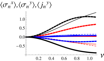
Figure 1: Some observables characterizing the NESS for an open $XXZ$ chain with Lindblad operators $L_{1}=2\sigma_{1}^{+}$, $L_{2}=L_{3}=0$,$L_{4}=\sqrt{2}\sigma_{N}^{-}$, $V=\nu(\sigma_{N}^{y}-i\sigma_{N}^{z})$, versus the amplitude $\nu$. Red, blue and black lines correspond to one-point correlations $\langle\sigma_{n}^{x}\rangle$ , $\langle\sigma_{n}^{y}\rangle$ and correlations $\langle j_{n}^{y}\rangle=2$ $\langle\sigma_{n}^{z}\sigma_{n+1}^{y}-\sigma_{n}^{y}\sigma_{n+1}^{z}\rangle$, respectively. Blue and red color: thick,thin,thick dashed, thin dashed lines correspond to $n=1,2,3,4$ respectively. Black color: thick,thin, and thick dashed lines stand for $\langle j_{n}^{y}\rangle$ at $n=1,2,3$. (note that $j_{n}^{y}$ is not conserved locally and is therefore depends on $n$). For $\nu=0$ the symmetry (20) is restored and all above observables vanish due to (22). The adopted parameter values are $N=4,J_{X}=J_{Y}=1,J_{Z}=-1.3$.

A different choice of the Lindblad operators, namely $L_{1,2}=\sqrt{\Gamma(1+\mu)}(\sigma_{1}^{y}\pm i\sigma_{1}^{z})$ and $L_{3,4}=$ $\sqrt{\Gamma(1-\mu)}(\sigma_{N}^{z}\pm i\sigma_{N}^{x})$ amounts to set a boundary twisting gradient in the $XY$-plane: the P–symmetry (20) is violated, but other symmetries appear, predicting a phenomenon of a sign alternation of the magnetization current with the system size (see Lindblad2011 , PopkovXYtwist ). For specific solvable cases, the full NESS of a $XXZ$ spin chain (30) with Lindblad driving at the edges can be obtained analytically, see ProsenExact2011 ,MPA2013 .

V.2 Spin and thermal conductance with boundary gradients

There is a large interest in studying the conductance in low-dimensional materials, due to the rich and often counterintuitive features they exhibit. In this section we discuss in full generality how one can switch on and off the magnetization and the energy currents by a suitable choice of boundary reservoirs , i.e. Lindblad operators, acting on the $XXZ$ spin chain (30).

Let us couple the $XXZ$ chain at the boundaries to baths of constant (but different) magnetizations, so that the time evolution of the state becomes dissipative and is described by LME

$$\frac{\partial\rho}{\partial t}=-i\left[H,\rho\right]+\Gamma(\mathcal{L}_{L}[\rho]+\mathcal{L}_{R}[\rho]),$$ (34)

where $H$ is the $XXZ$ Hamiltonian of the open $XXZ$ chain with anisotropy $\Delta$ (see Eq. (30)) . $\mathcal{L}_{L}[\rho]$ and $\mathcal{L}_{R}[\rho]$ are Lindblad dissipators $\mathcal{L}[\rho]=\sum_{k}L_{k}\rho L_{k}^{\dagger}-\frac{1}{2}\{\rho,L_{k}^{\dagger}L_{k}\}$ acting on the leftmost ($k=1$) and on the rightmost ($k=N$) boundary spins, while $\Gamma$ denotes the interaction rate with the dissipators. By choosing different parameter values of the boundary Lindblad dissipators $\mathcal{L}_{L}[\rho]$ and $\mathcal{L}_{R}[\rho]$, spin gradients can be introduced. In particular, the Lindblad dissipators target spin polarizations at site $1$ and at site $N$, described by the one-site density matrices $\rho_{L}$ and $\rho_{R}$ satisfying $\mathcal{L}_{L}[\rho_{L}]=0$, $\mathcal{L}_{R}[\rho_{R}]=0$, respectively. For sufficiently large values of $\Gamma$ the reduced density matrix of the system $\rho(t)$ evolves in time towards a nonequilibrium steady state density matrix, $\rho_{NESS}$, such that $Tr_{2,3,...N}\rho_{NESS}\rightarrow\rho_{L}$ and $Tr_{1,2,...N-1}\rho_{NESS}\rightarrow\rho_{R}$.

Let us choose the following Lindblad operators: for the left boundary, $\mathcal{L}_{L}$ dissipator contains operators

$$L_{1} =\sqrt{A}(\sigma_{1}^{y}-i\sigma_{1}^{z}),$$ (35)

$$L_{2} =\sqrt{\alpha}(\sigma_{1}^{z}+i\sigma_{1}^{x}),$$ (36)

and for the right boundary, $\mathcal{L}_{R}$ contains

$$L_{3} =(\sigma_{N}^{y}+i\sigma_{N}^{z}),$$ (37)

$$L_{4} =\sqrt{A\alpha}(\sigma_{N}^{z}-i\sigma_{N}^{x}).$$ (38)

We assume also that $A\neq 1$ and $0\leq\alpha\leq 1$. It is straightforward to check that $\mathcal{L}_{L}[\rho_{L}]=0$ where $\rho_{L}=\frac{I}{2}+\frac{1}{2}\sum_{\beta}\sigma_{\text{target(L)}}^{\beta}\sigma^{\beta}$ with

$$\sigma_{\text{target(L)}}^{x}=-\frac{2A}{2A+\alpha};\text{ }\sigma_{\text{target(L)}}^{y}=\frac{2\alpha}{A+2\alpha};\text{ }\sigma_{\text{target(L)}}^{z}=0.$$ (39)

The entries of the set $\sigma_{\text{target(L)}}^{\beta}$ are targeted spin components at the left boundary. At the right boundary, the targeted spin components are

$$\sigma_{\text{target(R)}}^{x}=\frac{2}{2+\alpha A};\text{ }\sigma_{\text{target(R)}}^{y}=-\frac{2\alpha A}{1+2\alpha A};\text{ }\sigma_{\text{target(R)}}^{z}=0.$$ (40)

Graphs of the targeted spin components at the left and at the right boundaries for $A=2$ are shown in Fig.2.

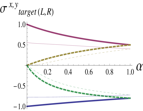
Figure 2: Targeted spin projections at the left and at the right boundary $\sigma_{\text{target(L)}}^{x},\sigma_{\text{target(R)}}^{x}$(upper and lower bold line, respectively), $\sigma_{\text{target(L)}}^{y},\sigma_{\text{target(R)}}^{y}$ (lower and upper dashed bold line, respectively) versus $\alpha$, from (39) and (40), with $A=2$. Thin full and dashed lines mark the actual values of boundary magnetizations from numerical LME solution, for the choice of parameters $A=2,N=5,\Delta=1,\Gamma=0.5$., see also Fig.3.

Due to the Heisenberg exchange interaction, one might expect that the presence of a spin gradient yields non-vanishing spin and heat currents, given by the Fourier law

$$j^{\gamma} =\chi_{\gamma\beta}\frac{\Delta s^{\beta}}{\Delta l}$$ (41)

$$J^{E} =\chi_{\beta}^{E}\frac{\Delta s^{\beta}}{\Delta l},$$ (42)

where $\Delta s^{\beta}/\Delta l=\langle\sigma_{N}^{\beta}-\sigma_{1}^{\beta}\rangle/(N-1)$ is the actual boundary gradient, $\chi_{\beta}^{E}$ and $\chi_{\gamma\beta}$ are transport coefficients, $\gamma,\beta=x,y,z$ and summation over repeated indexes is assumed. Note, that, due to quantum fluctuations, the actual average boundary magnetizations are only approximated by the respective targeted values, but do not coincide with them, $\sigma_{\text{target(L)}}^{\beta}\neq\langle\sigma_{1}^{\beta}\rangle$ (compare the bold and thin lines in Fig. 2), unless the rate $\Gamma$ becomes large. The overall qualitative behaviour of the actual $x$- and $y$- boundary gradients, at least for not very small $\Gamma$, is close to the targeted one, and yields applied gradients for all values of $0\leq\alpha\leq 1$ , see also Fig. 2. However, we find that for $\alpha=0$ the steady spin current is identically zero, $\langle j\rangle=0$ , while $\langle J^{E}\rangle\neq 0$. On the other hand, for $\alpha=1$ we obtain the opposite scenario, i.e. $\langle J^{E}\rangle=0$ and $\langle j\rangle\neq 0$. In fact, for $\alpha=0$ the stationary solution of the Lindblad equation $\rho_{NESS}$ is invariant under the following transformation,

$$\rho_{NESS}=\Omega_{x}\rho_{NESS}\Omega_{x}\,,$$ (43)

where $\Omega_{x}=(\sigma^{x})^{\otimes_{N}}$. Analogously, for $\alpha=1$, $\rho_{NESS}$ is invariant under the transformation

$$\rho_{NESS}=\Omega_{x}U_{rot}R\rho_{NESS}RU_{rot}^{\dagger}\Omega_{x}$$ (44)

where $R$ is again the left-right reflection, $(A\otimes B\otimes...\otimes C)=(C\otimes....\otimes B\otimes A)R$, and the diagonal matrix $U_{rot}=diag(1,i)^{\otimes_{N}}$ is a rotation in $XY$ plane: $U_{rot}\sigma_{n}^{x}U_{rot}^{\dagger}=$ $\sigma_{n}^{y}$, $U_{rot}\sigma_{n}^{y}U_{rot}^{\dagger}=-\sigma_{n}^{x}$. The Hamiltonian part of LME, $-i\left[H,\rho\right]$, is also invariant under both transformations, while for the Lindblad part the symmetries are satisfied due to the specific forms of $\mathcal{L}_{L}[\rho]$ and $\mathcal{L}_{R}[\rho]$ for $\alpha=0$ and $\alpha=1$.

Case $\alpha=0$. Making use of the symmetry (43) and of the properties of the Pauli matrices, we obtain the following expressions for the magnetization and for the energy currents (in what follows we use the shorthand notations $j$ and $J^{E}$ for these quantities),

$$j=Tr(\rho_{NESS}\hat{\jmath})=-Tr(\Omega_{x}\rho_{NESS}\Omega_{x}\hat{\jmath})=-j$$ (45)

$$J^{E}=Tr(\rho_{NESS}\hat{J}^{E})=Tr(\Omega_{x}\rho_{NESS}\Omega_{x}\hat{J}^{E})=J^{E}$$ (46)

The first one of these relations implies $j=0$, while no restrictions are imposed for $J^{E}$.

Case $\alpha=1$. We find the opposite situation: the energy current $J^{E}$ under the transformation (44) changes sign, while no restrictions are imposed for the magnetization current $j$. We conclude that $J^{E}=0$.

Case $0<\alpha<1$. For any intermediate value of $\alpha$, neither (43) nor (44) are satisfied. Consequently, both magnetization and energy currents are allowed to flow.

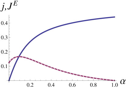
(a)

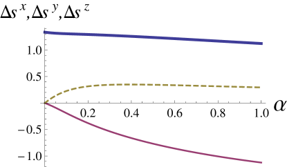
(b)

Figure 3: Panel(a): Steady magnetization current (line) and energy current (dashed line) as a function of $\alpha$, from the numerical solution of the Lindblad equation (34). Panel (b): Boundary $x,y,z$ gradients (thick, thin and dashed lines respectively) $\langle\sigma_{N}^{x}-\sigma_{1}^{x}\rangle,\langle\sigma_{N}^{y}-\sigma_{1}^{y}\rangle,\langle\sigma_{N}^{z}-\sigma_{1}^{z}\rangle,$ versus $\alpha$. Note that the targeted values of the boundary gradients fiven by difference of (40),(39). are different, see also Fig. 2, and in particular the targeted value of $\ z$-gradient is $0$. The adopted parameter values are $A=2,N=5,\Delta=1,\Gamma=0.5$.

In order to check our findings, we have obtained numerical solutions of LME (34) for small sizes $N$ and different values of the parameter $\Delta\neq 0$. In all cases we find complete agreement with theoretical predictions. A typical case is illustrated in Fig.3. For $A=1$, in addition we find that both $J_{\alpha=0,A=1}^{E}=0$ and $j_{\alpha=0,A=1}=0$, while only $j=0$ is predicted by the symmetry (43). Looking for an explanation, we readily find another symmetry of (34), valid for $A=1$ and $\alpha=0$:

$$\rho_{NESS}=\Omega_{x}R\rho_{NESS}R\Omega_{x}$$ (47)

which explains why also $J_{\alpha=0,A=1}^{E}=0$. In fact, it can be easily checked that under this symmetry the energy current operator changes sign, $R\Omega_{x}\hat{J}^{E}R\Omega_{x}=-\hat{J}^{E}$.

Various anomalities in the steady currents are often visible at the level of steady density profiles: e.g. ballistic current is usually accompanied by magnetization profiles which are flat in the bulk. One might wonder if the density profiles for our case, corresponding to the current anomalies at $\alpha=0,\alpha=1$ are special. For the point $\alpha=0$, the exact $y$- and $z$- magnetization profiles are trivial and flat, $\langle\sigma_{n}^{y}\rangle=$ $\langle\sigma_{n}^{z}\rangle=0$ for all $n$, a constraint, imposed by the symmetry (43), while the $x$- profile smoothly interpolates between the left and right boundary. On the other hand, for $\alpha=1$ we do not find any particularity in the magnetization profiles, which rather smoothly interpolate between the boundary values (even though this can be a finite-size effect), data not shown.

VI Conclusions

Transport properties of quantum systems can exhibit unexpected features if the nonequilibrium steady state has to obey certain symmetry properties. Various examples have been discussed in this paper for models of interacting systems of qubits, subject to local pumping mechanisms from specific Lindblad operators. We have first introduced different classes of these operators as spin-targeting and dephasing ones. Then, we have discussed the kind of symmetries they impose to the Lindblad master equation and to the corresponding nonequilibrium steady state. The important role played by parity symmetry selection rules has been illustrated for a general Hamiltonian model. These considerations have been also specialized to the XXZ spin chain model. We have shown that spin and energy currents can be suitably regulated by acting on the symmetries of the NESS through the parameters of the Lindblad operators. In particular, we find that both currents can vanish, even in the presence of finite applied gradients.

We have to point out that all the results reported in this manuscript rely on the basic assumption of uniqueness of the steady state solution of the Lindblad Master equation. Such a property applies to all the examples considered in this paper. An explicit check of this property can be performed by using the completeness criterion of the algebra generated by the Hamiltonian and by the Lindblad operators EvansUniqueness . Once the uniqueness is established, the nonequilibrium steady state is invariant under all the symmetries of the Lindblad master equation. In fact, any violation of a symmetry results in the existence of at least a one–parameter family of steady state solutions as a direct consequence of the linearity of the equation (34).

In a general perspective we can affirm that the properties of the steady states analyzed in this manuscript can be viewed as a first achievement in the exploration of new interesting features of the quantum Master equation. In Sec.V we have also shown an explicit example of how the vanishing of a current signals the presence of additional symmetries.

Acknowledgements. V.P. thanks the Center for Quantum Technologies, National University of Singapore, where this work was initiated, for the kind hospitality, and the Dipartimento di Fisica e Astronomia, Università di Firenze, for support through a FIRB initiative. R.L. would like to acknowledge financial support from the Italian MIUR-PRIN project n. 20083C8XFZ.

References

• (1) H.-P. Breuer and F. Petruccione, The Theory of Open Quantum Systems, Oxford University Press 2002.
• (2) M.B. Plenio and P.L Knight, Rev. Mod. Phys. 70, 101 (1998)
• (3) S. Diehl, A. Micheli, A. Kantian, B. Kraus, H. P. Buchler and P. Zoller, Nature Physics 4, 878 (2008)
• (4) B. Kraus, H. P. Buchler, S. Diehl, A. Micheli and P. Zoller, Phys. Rev. A 78, 042307 (2008)
• (5) F. Heidrich-Meisner, A. Honecker, and W. Brenig, Eur. Phys. J. Special Topics 151, 135 (2007), and references therein.
• (6) X. Zotos, J. Phys. Soc. Jpn. Supp. 74, 173 (2005) and references therein.
• (7) A. Klumper, Lect. Notes Phys. 645, 349 (2004).
• (8) X. Zotos, F. Naef and P. Prelovsek, Phys. Rev. B 55, 11029 (1997)
• (9) H. Wichterich, M. J. Henrich, H.P. Breuer, J. Gemmer and M. Michel, Phys.Rev. E 76 , 031115 (2007)
• (10) D.E. Evans, Comm. Math. Phys, 54, 293 (1977)
• (11) Gardiner C. W. and Zoller P., Quantum noise, Springer Verlag, Berlin (2000)
• (12) T. Prosen, New. J. Phys. 10, 043026 (2008).
• (13) B. Žunkovič and T. Prosen, J. of Stat. Mech. P08016 (2010).
• (14) G. Benenti, G. Casati, T. Prosen, D. Rossini and M. Žnidarič, Phys. Rev. B 80, 035110 (2009).
• (15) T. Prosen, Phys. Rev. Lett. 107, 137201 (2011).
• (16) S. Jesenko and M. Žnidarič, Phys Rev. B 84, 174438 (2011).
• (17) G. Benenti, G. Casati, T. Prosen and D. Rossini, Europhys. Lett. 85, 37001 (2009)
• (18) T. Prosen and B. Žunkovič, New J. of Phys. 12, 025016 (2010)
• (19) M. Žnidarič, Phys. Rev. E 83 011108 (2011)
• (20) T. Prosen and M. Žnidarič, Phys. Rev. Lett. 105, 060603 (2010).
• (21) M. Žnidarič, J. Stat. Mech. L05002 (2010); J. Phys. A 43 415004 (2010)
• (22) V. Popkov, M. Salerno and G. M. Schütz, Phys. Rev. E 85, 031137 (2012)
• (23) V. Eisler, J. of Stat. Mech., P06007 (2011)
• (24) T. Prosen, Phys.Rev.Lett. 109, 090404 (2012); T. Prosen, Phys.Rev. A 86 , 044103 (2012)
• (25) T. Prosen, Phys. Scr. Lett. 86, 058511 (2012).
• (26) NESS for $XXZ$ model enjoys full rotational symmetry around the $z$-axis, represented by unitary operator $U(\beta)=\exp(i\beta\sum_{k}\sigma_{k}^{z})$ , $\rho_{NESS}=U(\beta)\rho_{NESS}U(-\beta)$. The $P$- symmetry (20) is a particular reduction of the $U(\beta)$ for $\beta=\pi/2$.
• (27) Another equivalent symmetry $\rho_{NESS}=(\sigma^{y})^{\otimes_{N}}R\rho_{NESS}R(\sigma^{y})^{\otimes_{N}}$ is obtained as a product of (31) and (20).
• (28) M. Ali, A.R.P. Rau and G. Alber, Phys. Rev. A 81, 042105 (2010)
• (29) P. Krammer, H. Kampermann, D. Bruss, R.Bertlmann, L.C.Kwek and C. Macchiavello, Phys. Rev. Lett. 103, 100502 (2009)
• (30) M. Crammer, M.B. Plenio and H. Wunderlich, Phys. Rev. Lett. 106, 020401 (2011)
• (31) V. Popkov, J. Stat. Mech. (2012) P12015
• (32) D. Karevski, V. Popkov and G. M. Schütz, Phys. Rev. Lett. 110, 047201 (2013)