The planet search programme at the ESO CES and HARPS^,

Abstract

Context. In 1992 we began a precision radial velocity survey for planets around solar-like stars with the Coudé Echelle Spectrograph and the Long Camera (CES LC) at the 1.4 m telescope in La Silla (Chile) resulting in the discovery of the planet $\iota$ Hor b. We have continued the survey with the upgraded CES Very Long Camera (VLC) and the HARPS spectrographs, both at the 3.6 m telescope, until 2007.

Aims. In this paper we present additional radial velocities for 31 stars of the original sample with higher precision. The observations cover a time span of up to 15 years and permit a search for Jupiter analogues.

Methods. The survey was carried out with three different instruments/instrument configurations using the iodine absorption cell and the ThAr methods for wavelength calibration. We combine the data sets and perform a joint analysis for variability, trends, and periodicities. We compute Keplerian orbits for companions and detection limits in case of non-detections. Moreover, the HARPS radial velocities are analysed for correlations with activity indicators (CaII H&K and cross-correlation function shape).

Results. We achieve a long-term RV precision of 15 m/s (CES+LC, 1992–1998), 9 m/s (CES+VLC, 1999–2006), and 2.8 m/s (HARPS, 2003–2009, including archive data), respectively. This enables us to confirm the known planetary signals in $\iota$ Hor and HR 506 as well as the three known planets around HR 3259. A steady RV trend for $\epsilon$ Ind A can be explained by a planetary companion and calls for direct imaging campaigns. On the other hand, we find previously reported trends to be smaller for $\beta$ Hyi and not present for $\alpha$ Men. The candidate planet $\epsilon$ Eri b was not detected despite our better precision. Also the planet announced for HR 4523 cannot be confirmed. Long-term trends in several of our stars are compatible with known stellar companions. We provide a spectroscopic orbital solution for the binary HR 2400 and refined solutions for the planets around HR 506 and $\iota$ Hor. For some other stars the variations could be attributed to stellar activity, as e.g. the magnetic cycle in the case of HR 8323.

Conclusions. The occurrence of two Jupiter-mass planets in our sample is in line with the estimate of 10% for the frequency of giant planets with periods smaller than 10 yr around solar-like stars. We have not detected a Jupiter analogue, while the detections limits for circular orbits indicate at 5 AU a sensitivity for minimum mass of at least 1$M_{\mathrm{Jup}}$ (2$M_{\mathrm{Jup}}$) for 13% (61%) of the stars.

1 Introduction

The search for extra-solar planets has so far revealed approximately 850 exoplanets, most of them discovered by the radial velocity (RV) technique. Interestingly, many hot Jupiters have been found, a consequence related to the fact that the RV method as well as the transit method is more sensitive to short period planets. Out of 850 planets discovered so far, 65% have a period shorter than 1 year. Before the discovery of the first extrasolar planet around a solar-like star, the hot Jupiter 51 Peg b (Mayor & Queloz 1995), it was widely expected that planetary systems are in general similar to the solar-system and this was also predicted by most theoretical models as noted by Marcy et al. (2008). In the solar system, Jupiter is the dominant planet amongst all other planets and causes the largest RV amplitude. Therefore surveys were set up to search for planets with masses of 1 $M_{\mathrm{Jup}}$ and at distances of 5 AU from solar-like stars (e.g. Walker et al. 1995). The regime of Jupiter analogues is still sparsely explored because observations with long time-baselines and precise RV measurements are required; e.g. Jupiter orbits the Sun in 12 years and induces an RV semi-amplitude of 12 m/s.

There are many exoplanet search projects e.g. at Lick, AAT (O’Toole et al. 2009; Wittenmyer et al. 2011), Keck (Cumming et al. 2008), ELODIE/SOPHIE (Naef et al. 2005; Bouchy et al. 2009a), CORALIE (Ségransan et al. 2010), and HARPS (Naef et al. 2010; Mayor et al. 2011). These high precision RV projects have discovered a large fraction of the currently known planets and are continuously extending their time baselines. Examples for discovered Jupiter analogues are GJ 777Ab (Naef et al. 2003), a 1.33 $M_{\mathrm{Jup}}$ planet at 4.8 AU around a G6IV star, or HD 154345b (Wright et al. 2008), a 0.95 $M_{\mathrm{Jup}}$ planet at 4.5 AU around a G8V dwarf (all masses are $M\sin i$ minimum masses). Two more Jupiter-analogues were also recently reported by Boisse et al. (2012): HD150706b (2.7 $M_{\mathrm{Jup}}$, 7 AU) and HD222155b (1.9 $M_{\mathrm{Jup}}$, 5.1 AU).

The survey described in this paper was begun in 1992 (Endl et al. 2002) with the Coudé Echelle Spectrograph (CES) Long Camera (LC). With the advent of the CES Very Long Camera (VLC) in 1999, it was transferred to this instrument combination, and was continued in 2003 with the HARPS spectrograph. The last observations for this programme were taken in September of 2007, although we have also made use of archival data acquired up to 2009. The survey covers a time span of up to 15 years with RV precisions ranging from 15 m/s down to 2 m/s. A comparable survey was analysed by Wittenmyer et al. (2006) and carried out in the northern hemisphere with the 2.7 m telescope at the McDonald Observatory. It started in 1988 with 24 solar-like stars and 7 subgiants. When combined with CFHT data (Walker et al. 1995), it gave an even longer temporal coverage of up to 25 years, albeit with a somewhat lower precision (10–20 m/s).

2 The sample

The original sample of 37 solar-like stars was introduced in detail in Endl et al. (2002). Of these, the monitoring of six stars was stopped: HR 448, HR 753, HR 7373, Barnard’s star, Proxima Centauri, and GJ 433. The first three had been observed temporarily in 1996/97 as once promising metal rich targets, but were soon left out due to limited observing time. The latter three are M dwarfs which were included in a dedicated M dwarf survey with VLT+UVES. For these stars recent and more precise results are published in Zechmeister et al. (2009). So we are left with the 31 stars listed in Table 2 along with some of their properties (spectral type, visual magnitude, distance, and stellar mass).

Table 1: Targets with their spectral type SpT (Hoffleit & Jaschek 1991), visual magnitude $V$ (Perryman et al. 1997), distance $d$ (van Leeuwen 2007), secular acceleration $\dot{v}_{\mathrm{r}}$, and stellar mass $M$.

Star	alias	SpT	$V$ [mag]	$d$ [pc]	$\dot{v}_{\mathrm{r}}$ [m/s/yr]	$M$ [$M_{\odot}$]
HR77	$\zeta$ Tuc	F9V	4.23	8.59	0.84	1.06	[PM]
HR98	$\beta$ Hyi	G2IV	2.82	7.46	0.86	1.1	[D]
HR209	HR 209	G1V	5.80	15.16	0.01	1.10	[G]
HR370	$\nu$ Phe	F8V	4.97	15.11	0.16	1.20	[G]
HR506	HR 506	F9V	5.52	17.43	0.02	1.17	[G]
HR509	$\tau$ Cet	G8V	3.49	3.65	0.31	0.78	[T]
HR695	$\kappa$ For	G0V	5.19	21.96	0.02	1.12	[G]
HR810	$\iota$ Hor	G0V	5.40	17.17	0.06	1.25	[V]
HR963	$\alpha$ For	F8V	3.80	14.24	0.17	1.20	[G]
HR1006	$\zeta^{1}$ Ret	G2.5V	5.53	12.01	0.61	1.05	[G]
HR1010	$\zeta^{2}$ Ret	G1V	5.24	12.03	0.61	1.10	[G]
HR1084	$\epsilon$ Eri	K2V	3.72	3.22	0.07	0.85	[DS]
HR1136	$\delta$ Eri	K0IV	3.52	9.04	0.12	1.23	[PM]
HR2261	$\alpha$ Men	G6V	5.08	10.20	0.01	0.95	[G]
HR2400	HR 2400	F8V	5.58	36.91	0.02	1.20	[G]
HR2667	HR 2667	G3V	5.56	16.52	0.06	1.04	[G]
HR3259	HR 3259	G7.5V	5.95	12.49	0.30	0.90	[G]
HR3677	HR 3677	G0III	5.85	196.85	0.00	2.1	[G]
HR4523	HR 4523	G3V	4.89	9.22	0.53	1.04	[G]
HR4979	HR 4979	G3V	4.85	20.67	0.07	1.04	[G]
HR5459	$\alpha$ Cen A	G2V	-0.01	1.25	0.42	1.10	[P]
HR5460	$\alpha$ Cen B	K1V	1.35	1.32	0.40	0.93	[P]
HR5568	GJ 570 A	K4V	5.72	5.84	0.54	0.71	[G]
HR6416	HR 6416	G8V	5.47	8.80	0.22	0.89	[G]
HR6998	HR 6998	G4V	5.85	13.08	0.01	1.00	[G]
HR7703	HR 7703	K3V	5.32	6.02	0.37	0.74	[G]
HR7875	$\phi^{2}$ Pav	F8V	5.11	24.66	0.24	1.1	[PM]
HR8323	HR 8323	G0V	5.57	15.99	0.04	1.12	[G]
HR8387	$\epsilon$ Ind A	K4.5V	4.69	3.62	1.84	0.70	[G]
HR8501	HR 8501	G3V	5.36	13.79	0.19	1.04	[G]
HR8883	HR 8883	G4III	5.65	101.32	0.00	2.1	[G]

References for mass estimates: [D] Dravins et al. (1998), [DS] Drake & Smith (1993), [G] Gray (1988), [PM] Porto de Mello, priv. comm., [P] Pourbaix et al. (2002), [T] Teixeira et al. (2009), [V] Vauclair et al. (2008).

All stars have a brightness of $V<6$ mag and spectral types ranging from late F to K. There are two subgiant stars ($\beta$ Hyi and $\delta$ Eri) and two giant stars (HR 3677 and HR 8883) in the sample.

The sample includes six stars for which planet detections have been claimed. These are HR 506 (Mayor et al.), $\iota$ Hor (Kürster et al. 2000), $\epsilon$ Eri (Hatzes et al. 2000), HR 3259 (Lovis et al. 2006), HR 4523 (Tinney et al. 2011), and recently $\alpha$ Cen B (Dumusque et al. 2012). In Sect. 5 we provide more detailed information on individual objects and we will stress those planet hypotheses.

3 Instruments and data reduction

We used three high resolution spectrographs that are briefly described below with more detail provided for the less known VLC+CES. Table 2 gives an overview of some basic properties of the three instruments.

Table 2: The three used instruments/configurations with their wavelength reference, chosen spectral coverage and resolving power, and telescope diameter.

Spectrograph	Ref.	$\lambda$ [Å]	$R$	Tel.
CES + LC	I2	5367 – 5412	100 000	1.4 m
CES + VLC	I2	5376 – 5412	220 000	3.6 m
HARPS	ThAr	3800 – 6900	115 000	3.6 m

3.1 CES + Long Camera

In 1992 the survey started (1992-11-03 to 1998-04-04) with the Coudé Echelle Spectrograph (CES; Enard 1982) and its Long Camera (LC) fed by the 1.4 m Coudé Auxiliary Telescope (CAT) at La Silla (Chile). The CES+LC had a chosen wavelength coverage of 45 Å and a resolution of 100 000 (Table 2). A 2 k $\times$ 2 k CCD gathered part of one spectral Echelle order. An iodine gas absorption cell provided the wavelength calibration. More details about the instrument, data analysis, as well as the obtained results can be found in Endl et al. (2002). Table 3.1 lists the radial velocity results. The median rms is 15.2 m/s when excluding the giants and targets with companions and trends as commented in Table 3.1 and reflects the typical precision.

Table 3: Radial velocity results for all targets. For each instrument configuration the rms is calculated independently. RV data are not binned. Comments are on multiplicity (see also Table 5 for more information) and also indicate giants.

Listed are the number of observations $N$, the time baseline $T$, the weighted rms of the time series and the effective mean internal radial velocity error $\overline{\Delta RV}$.

3.2 CES + Very Long Camera

The Very Long Camera (VLC; Piskunov et al. 1997) of the Coudé Echelle Spectrograph (CES) was commissioned at the ESO 3.6 m telescope in La Silla (Chile) in April 1998 and decommissioned in 2007. The VLC was an upgrade of the CES that doubled the resolving power to $R=220\,000-235\,000$ as well as the CCD length so that 80% of the spectral coverage compared to the LC was retained (cf. Table 2). This upgrade together with improved internal stability, and also the larger telescope aperture promised an improvement of the RV precision. For our sample we collected VLC spectra from 1999-11-21 to 2006-05-24.

The VLC was fed by a fibre link from the Cassegrain focus of the 3.6 m telescope. A modified Bowen-Walraven image slicer provided an efficient light throughput at the high resolving power. It redistributed the light from the fibre with a 2″ aperture via 14 slices to an effective slit width of 0.16″ and resulted in a complex illumination profile in the spatial direction, i.e. perpendicular to the dispersion axis (Figs. 1 and 2). The right half of a 4 k $\times$ 2 k EEV CCD recorded part of one spectral order with the wavelength range of 5376 – 5412 Å. In 2000-06-15 CCD#59 was replaced by CCD#61 and in 2001-11-23 the CES fibre was exchanged.

The CES+VLC employed the same iodine cell as the CES+LC for wavelength calibration. This cell was controlled at a temperature of 50^∘C. The RV modelling (Sect. 3.4) requires a high resolution and high signal-to-noise iodine spectrum to reconstruct confidently the instrumental line profile (IP) of the spectrograph. In November 2008 we obtained a laboratory spectrum for our iodine cell with $R=925\,000$ and S/N$\sim$1000 using a Bruker IFS125HR high-resolution Fourier Transform Spectrometer (FTS) at Lund Observatory. A filament lamp was used as a background source. To limit the light from adjacent wavelength regions a set of filters were applied: a coloured glass filter type VG11, a notch-filter to reduce the internal laser light, and a hot mirror to suppress the red spectrum. While the iodine cell laboratory spectrum previously used by Endl et al. (2002) in their analysis of the CES LC data had only $R=400\,000$, the new scan ensures an iodine spectrum with a resolution almost 5 times higher than the resolution of the CES+VLC.

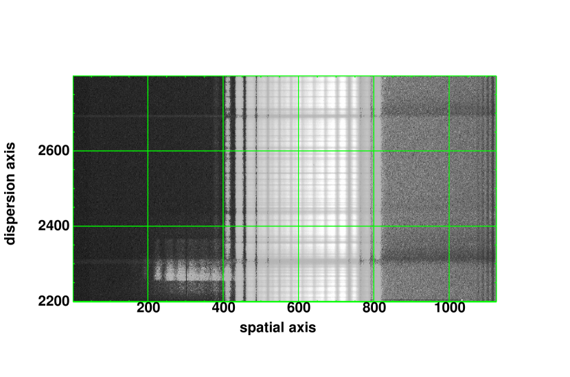
Figure 1: A small section of a VLC raw spectrum (star seen through the iodine cell; broad absorption features are stellar lines whereas narrow lines were introduced by the molecular iodine gas). The 14 slices span 400 pixels. The bright feature to the left near pixel row 2300 is a grating ghost. The area on the left side has a lower bias. The readout register is in the lower right corner of the chip (parallel clocking down, serial clocking to the right). Deeper stellar lines near row 2300 and 2700 have tails to the left and right. (The intensity scale is non-linear to bring out the discussed effects.)

Figure 2: Spatial profile of a VLC spectrum (cross-section for the rows 2400–2410 of the raw spectrum in Fig. 1; linear intensity scale).

The following properties of the CES+VLC spectra must be considered in the data analysis: The VLC spectra are contaminated by a grating ghost located in the middle of the CCD (Fig. 1) and suffered also from stray light produced by the image slicer. Ripples are visible in the continuum of high S/N ($\sim$1000) spectra caused by interference in the fibre. This can be seen, for instance, in flatfield exposures. Also visible in flats are less efficient rows on the chip every 512 pixels, due to a smaller pixel size resulting from the manufacturing process, which affect the wavelength solution. Moreover, as a peculiarity of the CES CCD electronics, a lower bias level is observed to the left of the spectra, caused by an electronic offset that occurs after processing a strong signal. This effect is attributed to the video amplifier electronics and requires the readout of several CCD rows to properly discharge (P. Sinclair, ESO, 2011, priv. comm.). Hence subsequent CCD rows are affected which may cause systematic spectral line asymmetries and RV shifts depending on the spectral line depth. Moreover, since the iodine lines are weaker, they may not receive the same shift as the stronger stellar lines and cannot correct completely for this effect.

The spatial profile has a width spanning more than 400 pixels offering a large cross-section for cosmic ray hits (so-called cosmics). For this reason the observing strategy aimed at three consecutive spectra in one night to be able to identify cosmics as outliers. However, we did not use this cosmics detection method because cosmics could also be efficiently identified as deviations from the spatial profile in the optimum extraction.

The VLC spectra were reduced with standard IRAF-tasks including subtraction of the overscan and a nightly master-bias, 2D flat-fielding, scattered light subtraction, and optimum extraction (Horne 1986) which also removes cosmics. The scattered light was defined left and right of the aperture with a low-degree polynomial used to interpolate across the aperture. This was done row-by-row and afterwards “smoothed” in the dispersion direction with a high-order spline to account for the above mentioned features and then as scattered light subtracted from the spectra. Finally, the science spectra were roughly calibrated with a nightly ThAr spectrum to provide an initial guess for the wavelength solution which is later refined with the iodine spectrum in the subsequent modelling process. The whole data reduction process largely removed the artefacts described above, however residual deviations are likely to still exist in the RVs of the VLC data. The typical precision is 9.4 m/s calculated as the median rms in Table 3.1 for the stars without comments.

3.3 HARPS

With HARPS we monitored our targets from 2003-11-06 to 2007-09-21 (2009-12-19 including archive data). The HARPS spectrograph is described in the literature (e.g. Mayor et al. 2003; Pepe et al. 2004). It is fibre fed from the Cassegrain focus of the 3.6 m telescope and located in a pressure and temperature stabilised environment. An optical fibre sends light from a ThAr lamp to the Cassegrain adapter for wavelength calibration. For the RV computation via cross-crorelation with a binay mask 72 Echelle orders ranging from 3800 Å to 6900 Å are available, a region much larger than for the CES.

We made use of the ESO advanced data products (ADP) to complement our time series which sometimes also extended the timebase. This archive provides fully reduced HARPS spectra including the final radial velocities processed by the pipeline DRS 3.5 (data reduction software). The radial velocities are corrected for the wavelength drift of the spectrograph (if measured by the simultaneous calibration fibre) and the RV uncertainty estimated assuming photon noise. The mean RV uncertainties range from 0.2 to 0.8 m/s and do not include calibration errors, guiding errors, and residual instrumental errors. For data analysis a stellar jitter term ($\geq$1.6 m/s) will be added in quadrature (see Sect. 4).

We recomputed with the HARPS DRS some of these archival RVs that suffered in the cross-correlation process from a misadjusted initial RV guess (off by more than 2 km/s) or from an inappropriate binary correlation mask. A different mask, e.g. K5 instead of G2, can produce RV shifts up to 20 m/s. The publicly available archive data originate from other programs such as short-term asteroseismology campaigns or the HARPS GTO (guaranteed time observations). The latter complemented our data with additional measurements, and in some cases provided a data set that outnumbers our own in terms of number of measurements and time base. We use only data taken in HARPS high accuracy mode (HAM), while we leave out data taken with iodine absorption cell or in high efficiency mode (EGGS, “Extra Good General Spectroscopy”) which uses a different fibre, a different injection method, and no scrambler and has a lower stability and a different zero point. Furthermore, spectra with a signal to noise of $\mathrm{S/N}<50$ are also left out.

The HARPS data provide an absolute RV scale which is shown in Figs. 19–23 and serves as our references frame into which the other instruments are transferred. Note that relative RV measurements are more precise than the absolute RVs (i.e. more precise than accurate). The median rms in Table 3.1 is 2.8 m/s for stars without comments. Note that several of our stars are active, so that this value is higher than the precision of 1 m/s usually quoted for HARPS.

To improve the combination of the HARPS and VLC data, spectra were taken in a few nights with both spectrographs immediately after each other making use of an easy switch possible with the common fibre adapter installed in May 2004.

3.4 Details of the RV computation for the CES+VLC data

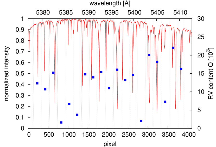
Figure 3: A VLC spectrum of $\tau$ Cet (without iodine cell) and the arrangement of the 200 pixel chunks with their individual $Q$-factors (blue squares). The intensity maximum of the spectrum is set to unity. The intensity declines to the edges due to instrumental effects (Blaze function).

To compute the RVs of the VLC spectra we used the AUSTRAL code described in Endl et al. (2000) which is based on the modelling technique outlined in Butler et al. (1996). The spectral order was divided into 19 spectral segments (chunks) with a size of 200 pixels (1.8 Å) which we empirically found to yield the optimal RV precision. The reasons could be that for smaller chunks the stellar RV information content becomes too small. For a larger chunk size, on the other hand, probably the assumption that the instrumental profile (IP) is constant over the chunk breaks down, or the discontinuities of the wavelength solution by the mentioned smaller and less efficient pixel rows are more problematic.

The stellar spectrum can be shifted across the CCD by several pixels due to the barycentric velocity of the Earth (calculated with the JPL ephemerides DE200, e.g. Standish 1990) and offsets in the instrument setup. To ensure that the same stellar lines fell in the same chunk, we shifted the chunks to the proper spectral location according to the barycentric correction (1 pixel is $\sim$ 500 m/s). So instead of having fixed chunk positions with respect to the CCD as originally implemented in the AUSTRAL code, this modification ensures always the same weighting factor for each chunk. The final wavelength solution in each chunk is provided by the iodine lines which record the instrumental drifts and offsets.

Figure 3 illustrates the alignment of the chunks with respect to the stellar spectrum. This placement of the chunks tries to avoid splitting up stellar lines between adjacent chunks. As one can see, the chunks contain only a few deep stellar lines or sometimes none. To quantify this, we calculated the quality factor $Q$ (Connes 1985; Butler et al. 1996; Bouchy et al. 2001) for each chunk in a stellar template. This factor sums in a flux-weighted way the squared gradients in a spectrum, hence measuring its RV information content. For photon noise, the estimated RV uncertainty is inversely proportional to $Q$, i.e. $\Delta RV\sim\frac{1}{Q}$. Hence, we weight each chunk RV with $Q^{2}$ when computing the RV mean. Chunks with $Q<7\,000$ were discarded (cf. Fig. 3, right axis). For comparison, the quality factor is $Q$=12857 for the whole spectral range in Fig. 3 and $Q=67\,000$ for an iodine spectrum (e.g. the spectrum of a featureless B-star taken through the iodine cell).

For $\tau$ Cet (GJ 71, HIP 8102, HR 509, HD 10700) which is known as an RV constant star (the HARPS data have an rms scatter of $\sim$1.1 m/s HARPS data, Pepe et al. 2011, this work), we achieve with the CES+VLC a long-term precision of 8.1 m/s (Fig. 19, Table 3.1). The internal RV errors of the individual spectra ($\sim$8.8 m/s), calculated as the errors of the mean RV of the chunks ($\mathrm{rms}/\sqrt{N_{\mathrm{chunk}}}$), are of the same order as the rms of the time series implying a fair error estimation.

3.5 Combining the LC and VLC data

The problem of instrumental offsets, i.e. different radial velocity zero points, occurs when data sets originate from different instruments (e.g. Wittenmyer et al. 2006) or after instrumental changes/upgrades. For instance, an offset of -1.8 m/s was reported by Rivera et al. (2010) after upgrading the Keck/HIRES spectrograph with a new CCD. An offset of only 0.9 m/s was mentioned by Vogt et al. (2010) when combining Keck and AAT data.

As described above we have used three different instruments/instrument configurations and we are also faced with the problem of the instrumental offset. There are basically two different methods for combining the data sets: (1) Simply fitting the offset, i.e. the data sets are considered to be completely independent and the zero points are free parameters in the model fitting. (2) If possible, measuring the offset physically by making use of some known relation between the data sets/instruments to keep the offset fixed.

In fact, we can measure the offset for the LC and VLC data albeit with a limited precision. The LC and VLC spectra were taken through the same iodine cell, i.e. the same wavelength calibrator. Because Endl et al. (2002) calculated the LC RVs with different stellar templates and an iodine spectrum of lower resolution than used in this work, we re-calculated the RVs for all LC spectra with the same VLC stellar template (which is shorter than the LC spectra) and the new iodine cell scan to have the same reference for the LC and VLC. The re-calculated RVs are verified to have a precision similar to the published LC data.

Then we computed the mean of the re-calculated LC and VLC time series. If a star has a constant RV, one would expect that the means of both time series are the same, i.e. the offset $\mathrm{\overline{RV}_{VLC}-\overline{RV}_{LC}}=0$ within the uncertainties of the means ($\sigma_{\mathrm{LC}}$ and $\sigma_{V\mathrm{LC}}$). This can be tested with the $t$-statistics, in particular Welch’s $t$-test (for two independent samples with unequal sizes and variances). We suggest that keeping the offset fixed is valid, if the quantity

$$t=\frac{\overline{RV}_{\mathrm{LC}}-\overline{RV}_{\mathrm{VLC}}}{s}\quad\text{with}\quad s=\sqrt{\frac{\sigma_{\mathrm{LC}}^{2}}{N_{\mathrm{LC}}}+\frac{\sigma_{V\mathrm{LC}}^{2}}{N_{\mathrm{VLC}}}}$$ (1)

is not rejected by the Null-hypothesis. The parameter $s$ is an estimate for the standard error of the difference in the means and is calculated from sample variances $\sigma_{i}^{2}$ and sample sizes $N_{i}$. The variable $t$ follows a $t$-distribution with $\nu$ degrees of freedom. For instance, for $|t|>1.7$ and $\nu>30$ the difference in the means is significant with a false alarm probability of FAP$<$10%. For some of our stars the FAP for the offset difference is not significant: $\delta$ Eri (64%), $\epsilon$ Eri (23%), HR 209 (92%), and HR 3259 (15%). However, from Fig. 4 it can be seen that there are also stars having significant offsets leaving doubts whether the offset can be kept fixed in general.

Figure 4 shows that for our sample an average offset of 10.4 m/s ($\pm$7.7 m/s) remains for the RV constant stars when comparing the RV means of the VLC and LC data. This offset might be due to systematics in the deconvolution process of the stellar template or in the modelling. For example, due to the different resolution, the LC data have to be modelled with a different chunk size (154 pixels to cover two VLC chunks). We corrected all re-calculated LC RVs for this systematic offset. Finally, we adjusted the RV mean of the published LC time series (Endl et al. 2002) to fit the RV mean of the re-calculated time series. In Figs. 19–23 the LC (Endl et al. 2002) and VLC data are always shown relative to each other with the measured and corrected offset (and not with a fitted RV offsets that could have been taken from our fit results presented below in Sect. 4) to conserve the true measurements.

The uncertainty of the offset found in the sample is rather large for it to be considered a fixed value. On the other hand the approximately known offset can hold important information, in particular in the case of HR 2400 or $\epsilon$ Ind A. Therefore we choose a compromise between a fixed offset and a free offset when fitting a function. Because one expects the difference of the zero point parameters to be zero ($c_{\mathrm{VLC}}-c_{\mathrm{LC}}\approx 0$), we introduce in the $\chi^{2}$-fitting a counteracting potential term $\eta^{2}$ (also called penalty function, e.g. Shporer et al. 2010), that increases when the zero point difference becomes larger

$$\hat{\chi}^{2}=\chi^{2}+\eta^{2}\quad\text{with}\quad\eta=\frac{c_{\mathrm{VLC}}-c_{\mathrm{LC}}}{s}.$$ (2)

The resulting $\chi^{2}$ (when minimising $\hat{\chi}^{2}$) will be higher compared to that obtained when fitting with free offsets but lower than for fixed offsets. The parameter $s$ determines the coupling between the offsets. After performing the fit it can be checked, if the fit has spread the zero points too much (if $\eta\gg 1$ or if there are large jumps in the model curves in Figs. 19–23). For $s$ we attributed the uncertainty of the offset correction of 7.7 m/s leading to a weak coupling.

It is worth mentioning, that in Bayesian analysis $\hat{\chi}^{2}$ can be identified with the likelihood when assuming a Gaussian distribution for the prior information that the expected zero point difference is zero.

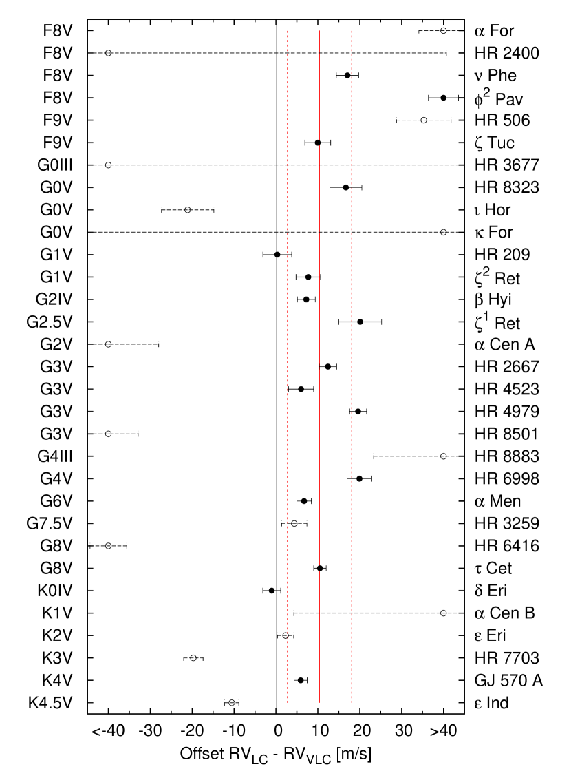
Figure 4: Difference between the means of the VLC and re-computed LC time series for all our stars ordered by spectral type. For RV constant stars (black filled circles) there occurs a systematic offset of 10.4$\pm$7.7 m/s (red solid line and red dashed lines). Stars shown with open circles were not included in the offset analysis (for reasons see comments in Table 3.1). The shown error bars correspond to the uncertainty in the means, i.e. parameter $s$ from Eq. (1).

3.6 Combining the CES and HARPS data

In principle, VLC and HARPS data could be combined in a similar way. They have different wavelength calibrators, but, since there are some nights with almost simultaneous observations (within minutes), they are closely related in time. The difference between these consecutive measurements should be zero so that it is tempting to bind directly the time series by means of those nights. However, this does not account for fluctuations due to the individual uncertainties. Again a coupling term would be a more secure approach.

However, for reasons of simplicity we choose a fully free offset between the HARPS and the CES data. Because the VLC and the HARPS time series overlap well this is less critical, in contrast to the LC and VLC time series which are separated by a 2-year gap. The relative offsets between the CES and HARPS data as illustrated in Figs. 19–23 correspond to the common best fitting model (constant, slope, sinusoid, or Keplerian; cf. Sect. 4).

4 Analysis of the radial velocities

In this section we describe our data analysis and the general results of the survey, while some individual objects are discussed in detail in Sect. 5. The tests which we perform hereafter were repeated on the residuals of the binaries and planet hosting stars to search for additional companions and are indicated as objects with index r in Table 4.2.

4.1 Preparation of RV data and jitter consideration

Before the data analysis we binned the data into 2-hr intervals by calculating weighted means for the temporal midpoint, RV, and RV error. The 2-hr interval will especially down-weight nights from asteroseismology campaigns (see Sect. 3.3) and reduce the impact of red noise (Baluev 2012), while resulting in nightly averages for most other nights and still permitting to search for planets with periods as short as one day. Such intervals are also employed for solar-like stars (e.g. Rivera et al. 2010) to average out the stellar jitter, i.e. intrinsic stellar RV variation caused by, e.g., oscillation or granulation in the atmospheres of the stars. While the Sun has an oscillation timescale of $\sim$5 min, its granulation has lifetime $\lesssim$25 min (see Dumusque et al. 2011b for adequate observing strategies). However note, that in our own survey we have usually taken three consecutive spectra in one night covering in total only 5–10 min, which is not sufficient to average out all those intrinsic stellar RV variations. To investigate the short-period jitter, we calculated the weighted scatter in each 2-hr bin with at least 2 measurements and then the weighted mean of these scatters. Table A lists the jitter estimate $\sigma_{\mathrm{jit},\tau}$ from the HARPS data for each star and the mean time scale $\tau$ accessible for this estimate within the 2 h bins. Note that these time scales may not sufficiently cover the real jitter time scale in all cases. Therefore these estimated jitter values were not used in a further analysis.

There can be also a long-term jitter with time scales of few days to weeks related to the rotation period (due to the appearance and disappearance of spots) or up to few years due to the magnetic cycle of a star. Isaacson & Fischer (2010) provide jitter estimates as a function of $B-V$ colour and chromospheric activity index $S_{\mathrm{HK}}$ based on Keck observations for more than 2600 main sequence stars and subgiants. Using these relations and the median $S_{\mathrm{HK}}$ values in the HARPS data (which in most cases agree well with other literature values; see Table A), we estimate the jitter $\sigma_{\mathrm{jit,long}}$ for our stars (Table A). The jitter terms are usally $\gtrsim 2$ m/s. For GJ 570 A and $\epsilon$ Ind A the expected jitter is only 1.6 m/s. Both are K dwarfs with $1.0<B-V<1.3$ and, according to Isaacson & Fischer (2010), those stars have the lowest level of velocity jitter decoupled from their chromospheric activity. The jitter terms $\sigma_{\mathrm{jit,long}}$ were added in quadrature to the internal errors for all stars and lead to a more balanced fit with the CES data. Morevover, to cross-check whether detected RV signals might be caused by those kinds of stellar activity we will also analyse in the HARPS data correlations between the RV data and activity indicators such as Ca II H&K emission and variations of the bisector (BIS) and the FWHM of the cross-correlation profile (Sect. 4.5). All RVs and HARPS activity indicators are online available.

In fitting the data we accounted for the secular acceleration of the RVs (as given in Table 2). This perspective effect can become a measurable positive trend in some high proper motion stars (Schlesinger 1917; Kürster et al. 2003; Zechmeister et al. 2009). In our sample, $\epsilon$ Ind A has the highest secular acceleration with 1.8 m/s/yr. Its contribution is depicted in Fig. 23 by a dashed line.

4.2 Excess variability

To investigate objects for excess variability it is common to compare the observed scatter with a noise estimate. A significantly larger scatter indicates variability. Because internal errors $\Delta RV_{i}$ and jitter estimations $\sigma_{\mathrm{jit}}$ are available, the quality of each measurement is assessed and allows us to weight the measurements in the $\chi^{2}$-statistics, $w_{i}=\frac{1}{\sigma_{i}^{2}}=\frac{1}{\Delta RV_{i}^{2}+\sigma_{\mathrm{jit}}^{2}}$. As the scatter we calculate the weighted rms which is here defined as

$$\mathrm{rms}=\sqrt{\frac{N}{N-\nu}\frac{1}{W}\sum_{i=1}^{N}\frac{(RV_{i}-f(t_{i}))^{2}}{\sigma_{i}^{2}}}=\sqrt{\frac{N}{N-\nu}\frac{\chi^{2}}{W}}$$ (3)

where $W=\sum w_{i}$ is the sum of the weights and $\nu$ the number of model parameters. Outliers with a large uncertainty will contribute less to the rms. The factor $\frac{N}{N-\nu}$ is a correction that converts the uncorrected and biased variance into an unbiased variance, i.e. to have an unbiased estimator for the population variance. In the unweighted case ($w_{i}=1$, $W=N$) we obtain the well known formula for the unbiased rms: $\mathrm{rms}=\sqrt{\frac{1}{N-\nu}\sum(RV_{i}-f(t_{i}))^{2}}$.

Furthermore, we define the weighted mean noise term $\sigma$ via the mean of the weights

$$\sigma=\frac{1}{\sqrt{\langle w_{i}\rangle}}=\sqrt{\frac{N}{W}}=\sqrt{\frac{N}{\sum_{i=1}^{N}\frac{1}{\sigma_{i}^{2}}}}.$$ (4)

Again lower-quality measurements will contribute less to the mean noise level.

With these definitions the reduced $\chi^{2}$ can be easily expressed as the ratio of weighted rms to weighted mean noise level

$$\chi_{\mathrm{red}}^{2}=\frac{\chi^{2}}{N-\nu}=\frac{\mathrm{rms}^{2}}{\sigma^{2}}.$$ (5)

To test for excess variability we have to fit a constant and to calculate the scatter around the fit. For the joint analysis we account for the zero point parameter of each data set when fitting a constant as outlined in Sect. 3.5. Note that the probability for the excess variability $\mathrm{Prob}(\chi_{\mathrm{red}}^{2})$ is directly reliant on a proper estimate for the noise level $\sigma$. Also note that the tests in the next sections employ model comparisons and the jitter estimate enters only indirectly through fitting with modified weights. Table 4.2 summarises for the combined data set the weighted noise term $\sigma$, the weighted rms, and the $\chi^{2}$-probability for this test. Table A lists additionally the individual rms (columns 5-7 labelled $\mathrm{rms}_{\mathrm{constant}}$) for each instrument. These values can differ from Table 3.1, because in Table 4.2 secular acceleration is accounted for, jitter has been added, the data are binned, and the LC and VLC offsets are coupled. Because the HARPS data have a much higher precision, they dominate the statistics.

Table 4: Summary of the tests for excess variability, slope, and periodicities (sinusoidal and Keplerian) for the combined data set. Significant trends and sinusoidal periods are printed in bold face (FAP$<1$‰). An index “r” to the name of the star (first column) indicates tests on the residuals as derived from the most significant model to the original data.

Listed are the number of binned observations $N_{\mathrm{bin}}$, the combined time baseline $T$, the mean combined noise term $\sigma$ (including jitter), the combined weighted rms of the time series, the flag S for the probable main source of the RV variations as concluded in this work in Sect. 5 (A - activity, B - binary/wide stellar companion, P - planet), the $\chi^{2}$-probability for fitting a constant, and the false alarm probabilities (FAP) for the other tests. Also listed are the weighted scatter of the residuals (rms_slope, rms_sin, rms_Kep) and some best-fitting parameters (slope and the periods $P_{\mathrm{sin}}$ and $P_{\mathrm{Kep}}$).

The small $\chi^{2}$-probabilities for most of the stars indicate that they are variable with respect to our noise estimate $\sigma$. However, 10 stars (and the RV orbit residuals of 8 stars) have $\mathrm{Prob}(\chi^{2})>1\%$, i.e. they show only low or no excess variability. In five cases the scatter is smaller than the noise level, i.e. $\chi_{\mathrm{red}}^{2}<1$, implying an overestimation of the noise level. Indeed, for four stars ($\zeta$ Tuc, $\tau$ Cet, HR 2667, and HR 6998) the jitter estimate $\sigma_{\mathrm{jit,long}}$ in Table A is higher than the scatter of the HARPS measurements (Table A). The reason for jitter overestimation might be a somewhat lower precision of the Keck sample from which the jitter relation was derived (Isaacson & Fischer 2010).

4.3 Long-term trends

Because potential planets or companions can have orbital periods much longer than our observations, these objects may betray themselves by a trend in the RVs. We searched for trends by fitting a slope to the data and derived its significance via the fit improvement with respect to the constant model (previous Sect.) via

$$F_{\mathrm{slope}}=(N-4)\frac{\chi_{\mathrm{constant}}^{2}-\chi_{\mathrm{slope}}^{2}}{\chi_{\mathrm{slope}}^{2}}$$ (6)

or when expressed with unbiased weighted variances

$$F_{\mathrm{slope}}=\frac{(N-3)\,\mathrm{rms}_{\mathrm{constant}}^{2}-(N-4)\,\mathrm{rms}_{\mathrm{slope}}^{2}}{\mathrm{rms}_{\mathrm{slope}}^{2}}.$$ (7)

The associated probability for this $F$-value follows a $F_{1,N-4}$-distribution (4 parameters: 1 slope, 3 zero points). Again Table 4.2 summarises the test for long-term trends. When adopting a false alarm probability threshold of $<10^{-3}$ fitting a slope improves significantly the rms of all binaries as well as that of $\beta$ Hyi, $\tau$ Cet, GJ 570 A, $\epsilon$ Ind A and the residuals of HR 506. We note that for $\beta$ Hyi, $\alpha$ For, GJ 570 A, HR 6416, HR 7703, $\epsilon$ Ind A, and HR 8501 the trend is a sufficient model (regarding sinusoid and Keplerian fit, see next Section), because of the smaller FAP or weighted rms (i.e. smaller $\chi_{\mathrm{red}}^{2})$. For these stars the trend is depicted in Figs. 19–23.

Some of our stars have known wide visual companions with a known separation $\rho$ listed in Table 5. Whether these objects are able to cause the observed trend, can be verified by the estimate ($|\ddot{\@vec{r}}_{\mathrm{A}}|=G\frac{m_{\mathrm{B}}}{r^{2}}$)

$$m_{{}_{\mathrm{B}}}\sin i\geq\frac{|\ddot{z}_{\mathrm{A}}|r^{2}}{G}\geq\frac{|\ddot{z}_{\mathrm{A}}|\rho^{2}}{G}=5.6\cdot 10^{-3}M_{\mathrm{Jup}}\frac{|\ddot{z}_{\mathrm{A}}|}{\mathrm{m/s/yr}}\left(\frac{\rho}{\mathrm{AU}}\right)^{2}$$ (8)

with the radial acceleration $|\ddot{z}_{\mathrm{A}}|\leq|\ddot{\@vec{r}}_{\mathrm{A}}|\sin i$ of the observed component A and the projected separation $\rho\leq r$ between both components. For comparison, Jupiter at 5.2 AU can accelerate the Sun by 6.6 m/s/yr. Table 5 summaries the information about known wide companions and shows that the minimum companion masses derived from the measured slopes are below 0.5 $M_{\odot}$ for $\alpha$ For, GJ 570 A, HR 6416, HR 7703, and HR 8501. These masses are in agreement with the masses as expected from the spectral type of their companions. However, $\epsilon$ Ind B cannot explain the trend seen for $\epsilon$ Ind A (see Sect. 5 for details).

The other possibility for a trend is an unknown and unseen companion. Whether the strength and the long duration of a trend is still compatible with a planetary companion, can be estimated more conveniently, when Eq. (8) is expressed in terms of the orbital period $P$ which is also unknown but has to be (for circular orbits) at least twice as large as the time span of observations $T$. With Kepler’s 3^rd law $\frac{a^{3}}{P^{2}}=G\frac{M+m}{4\pi^{2}}$, Eq. (8) can be written as

$$m_{\mathrm{B}} \sin i\geq G^{-1/3}|\ddot{z}|\left(\frac{P}{2\pi}\right)^{4/3}\left(M_{\mathrm{A}}+m_{\mathrm{B}}\right)^{2/3}$$

$$=5.6\cdot 10^{-3}M_{\mathrm{Jup}}\frac{|\ddot{z}|}{\mathrm{m/s/yr}}\left(\frac{P}{\mathrm{yr}}\right)^{4/3}\left(\frac{M_{\mathrm{A}}+m_{\mathrm{B}}}{\mathrm{M}_{\odot}}\right)^{2/3}$$ (9)

For $\epsilon$ Ind A we find its companion to have $m\sin i\gtrsim 0.97\,M_{\mathrm{Jup}}$ for $P>30$ yr.

Table 5: Information about wide companions. Listed are separation $\rho$, period estimate $P$, references, and our estimates for minimum masses $M_{\min}$ derived via Eq. (8) from the slope of the linear fit to the data (Table 4.2) and $\rho$. For minimum masses in brackets the trends were not significant.

Star	Companion	$\rho$ [″]	$\rho$ [AU]	$P$ [yr]	Ref.	$M_{\min}$ [$M_{\mathrm{Jup}}$]	further companions
$\alpha$ For	GJ 127 B (G7V)	4.4	62	314	[BP, H, P]	248
$\alpha$ Men	HD 43834 B (M3.5)	3.05	31		[E]	(1)
HR 2667	GJ 9223 B (K0V)	20.5	332		[F, WD]	(191)
HR 4523	GJ 442 B (M4V)	25.4	234		[P]	(3)
GJ 570 A	GJ 570 BC (M1.5V+M3V)	24.7	146		[B]	325	GJ 570 D (T, 258$\aas@@fstack{\prime\prime}$3)
HR 6416	GJ 666 B (M0V)	10.4	92	550	[LH, P]	446	GJ 666 C (M6.5V, 41$\aas@@fstack{\prime\prime}$8)
							GJ 666 D (M7V, 40$\aas@@fstack{\prime\prime}$7)
HR 7703	GJ 783 B (M3.5)	7.1	43		[P]	38
$\epsilon$ Ind A	GJ 845 Bab (T1+T6)	402.3	1459		[S]	28130
HR 8501	GJ 853 B ($V<10$ mag)	2.5–3.4	41		[M, WD]	163

References: [BP] Baize & Petit (1989), [B] Burgasser et al. (2000), [E] Eggenberger et al. (2007), [F] Favata et al. (1997), [H] Heintz (1978), [LH] Luyten & Hughes (1980), [M] Mason et al. (2001), [P] Poveda et al. (1994), [S] Scholz et al. (2003), [WD] Worley & Douglass (1997).

4.4 Search for Periodicities and Keplerian orbits

To search for the best-fitting sinusoidal and Keplerian orbits, we employed the generalised Lomb-Scargle (GLS) algorithm described in Zechmeister & Kürster (2009). It was adapted to treat all three data sets with different offsets and also incorporates the weak offset coupling described before (Sect. 3.5). Searching for sine waves is a robust method to find periodicities and orbits with low eccentricities, while for highly eccentric orbits the Keplerian model should be applied.

Figures 5, 12, 13, 14, and 15 show the periodograms for some of the stars discussed here. The periodograms are normalised as

$$p=\frac{\chi_{\mathrm{constant}}^{2}-\chi_{\mathrm{sin}}^{2}}{\chi_{\mathrm{constant}}^{2}}\quad\mathrm{and}\quad p_{\mathrm{Kep}}=\frac{\chi_{\mathrm{constant}}^{2}-\chi_{\mathrm{Kep}}^{2}}{\chi_{\mathrm{constant}}^{2}}.$$ (10)

involving the $\chi^{2}$ of the constant, sinusoidal, and Keplerian model, respectively. Analogous to Cumming et al. 2008 and Zechmeister & Kürster (2009), we calculated the probabilities of the power values for the best-fitting sinusoid and Keplerian orbit ($p_{\mathrm{best}}$ and $p_{\mathrm{Kep,best}}$) via

$$\mathrm{Prob}(p>p_{\mathrm{best}}) =(1-p_{\mathrm{best}})^{\frac{N-5}{2}}\quad\mathrm{and}$$ (11)

$$\mathrm{Prob}(p_{\mathrm{Kep}}>p_{\mathrm{Kep,best}}) =(1+\tfrac{N-7}{2}p_{\mathrm{Kep,best}})(1-p_{\mathrm{Kep,best}})^{\frac{N-7}{2}},$$ (12)

respectively. Compared to the probability functions given by these authors which account for one offset, here are slight modifications in the equations (numerator in the fractional terms decreased by 2) arising from the three zero points, i.e. two more free parameters.

The final false alarm probability (FAP) for the period search accounts for the number of independent frequencies $M$ with the simple estimate $M\approx fT$ (Cumming 2004), i.e. the frequency range $f$ and the time baseline $T$, and is given by

$$\mathrm{FAP}=1-[1-\mathrm{Prob}(p>p_{\mathrm{best}})]^{M}$$ (13)

and can be approximated by $\mathrm{FAP}\approx M\cdot\mathrm{Prob}(p>p_{\mathrm{best}})$ for $\mathrm{FAP}\ll 1$. Since our frequency search interval ranges from 0 to 1 d^-1, we have typically $M\sim 5500$ for a 15 year time baseline.

Table 4.2 summarises the formal best-fitting sinusoidal and Keplerian periods ($P_{\mathrm{sin}}$ and $P_{\mathrm{Kep}}$) found by the periodograms along with their residual weighted rms and FAP. Our approach recovers all stars that exhibit long-term trends emulated by long periods and generally decreases the rms down to a few m/s.

We identify for HR 506, $\iota$ Hor, and HR 3259 the same periods that were previously announced as planetary signals (Kürster et al. 2000, Mayor et al.⁵, Lovis et al. 2006). In Sect. 5 we derive for HR 506 and $\iota$ Hor refined orbital solutions (see also Table 6 and 7) and investigate the correlation between RV and activity indicators.

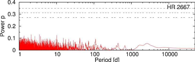
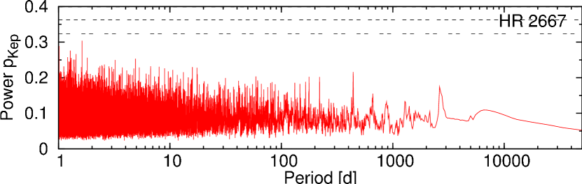
Figure 5: GLS (top) and Keplerian (bottom) periodogram for HR 2667 which is constant to 3.1 m/s. The horizontal lines mark the $10^{-2}$, $10^{-3}$, and $10^{-4}$ false alarm probabilities (FAP).

For the refinement of the orbital parameters and the error estimation we used the program GaussFit (Jefferys et al. 1988) which can solve general nonlinear fit-problems by weighted least squares and robust estimation. As initial guess we provided the parameters found with the Keplerian periodogram in the previous section. All offsets were free parameters.

We provide also a first orbital solution for the spectroscopic binary HR 2400 (Table 8). However, for $\kappa$ For, $\alpha$ Cen A+B and the giant HR 3677 it is not possible to give a reliable orbital solution since our measurements cover only a small piece of their orbits. Companion masses are estimated in Sect. 5.

4.5 Correlations with Ca II H&K, BIS, and FWHM

Radial velocity variations can be caused by stellar variability such as oscillations, granulations, spots, and magnetic activity cycles. They can affect the stellar line profile and, in case of spots and magnetic cycles, also the amount of Ca II H&K emission. To test this, one can analyse the $R^{\prime}_{\mathrm{HK}}$-index and the shape of the cross-correlation function (CCF) function in particular its full width at half maximum (FWHM) and bisector span (BIS, Queloz et al. 2001) which are measures for the averaged stellar line width and asymmetry, respectively. The activity indicators are products of the HARPS pipeline and the computation of ($S_{\mathrm{HK}}$ and) $R^{\prime}_{\mathrm{HK}}$ is described in Lovis et al. (2011). Note that these indicators do not cover the whole survey, because they cannot be derived from the CES spectra (which do not include the Ca II region and are contaminated by the iodine lines). The $S_{\mathrm{HK}}$ errors are derived from photon noise (Lovis et al. 2011), the BIS span errors are taken as twice the internal RV errors, and the FWHM errors are 2.35 times the internal RV errors.

The time series of the activity indicators and their correlations with RVs are shown for each star in Figs. 25–57. Tables A and A summarise for each star and activity indicator their mean values, scatter, and the correlation coefficients. Statistically significant linear correlations with $\mathrm{FAP}<0.01$ are highlighted in bold font in the Tables and depicted by a solid line in the Figures.

Note that a high statistical correlation does not necessarily mean a physical correlation, in particular when both quantities exhibit just trends which could coincide just by chance and temporarily. However, if the correlation is present during more complex temporal variations, e.g., both quantities have the same period, a planetary hypothesis should be excluded. But note also, that the Sun hosts a Jupiter in a 12 yr orbit and shows a comparably long magnetic cycle (11 yr).

In the sample, $\tau$ Cet has the smallest variations in $\log R^{\prime}_{\mathrm{HK}}$ (0.005 dex), while $\zeta^{1}$ Ret has the largest variations (0.048 dex). We find significant correlations between RV and $\log R^{\prime}_{\mathrm{HK}}$ for the stars $\beta$ Hyi, HR 209, $\zeta^{1}$ Ret, $\alpha$ Men, HR 4979, HR 8323, and for the two stars with planet candidates $\iota$ Hor and $\epsilon$ Ind A. However, the correlation seen for $\alpha$ Cen B (probably also HR 7703 and $\epsilon$ Ind A) is artificial since the RV trend is largely caused by a wide companion, respectively, instead of a magnetic cycle (Sect. 5).

Lovis et al. (2011) provide also a relation to estimate the slope of the RV and $R^{\prime}_{\mathrm{HK}}$ correlations based on the stellar temperature $T_{\mathrm{eff}}$ and metallicity [Fe/H]. After conversion to a slope w.r.t. $\log R^{\prime}_{\mathrm{HK}}$ by multiplication with a factor of $\ln 10\cdot R^{\prime}_{\mathrm{HK}}/10^{5}$, these estimates can be compared to the derived slopes given in Table A. As an additional cross-check, we will do this comparison occasionally in Sect. 5 when we conclude for a magnetic cycle hypothesis. We note that eight stars were included also in a sample analysed by Lovis et al. (2011) for magnetic cycles via $R^{\prime}_{\mathrm{HK}}$. With the exception of the RV standard star $\tau$ Cet and the subgiant $\delta$ Eri, these authors reported $R^{\prime}_{\mathrm{HK}}$ cycles/trends for these stars.

Significant correlations between RV and BIS are found for 7 stars ($\tau$ Cet, $\iota$ Hor, $\epsilon$ Eri, $\alpha$ Men, HR 4979, HR 8323, and HR 8883). The correlation for three more stars ($\alpha$ Cen B, GJ 570 A, and HR 8501) should be artificial, since the RV trends can be attributed to a wide stellar companion.

Finally, RV-FWHM correlations are found for 7 stars ($\beta$ Hyi, HR 209, $\tau$ Cet, $\zeta^{1}$ Ret, $\zeta^{2}$ Ret, $\alpha$ Men, and HR 8323). For 6 other stars (HR 2400, HR 3677, $\alpha$ Cen A, $\alpha$ Cen B, GJ 570 A, and probably also $\epsilon$ Ind A) the correlations are artificial due the RV trends caused by their wide companions.

RV variations caused by the magnetic cycle should result in positive correlations with all three indicators (Lovis et al. 2011). The stars $\alpha$ Men and HR 8323 are nice showcase examples for this effect. On the other hand, an RV-BIS anti-correlation (cf. the active stars $\iota$ Hor, $\epsilon$ Eri, and also the giant HR 8883) is expected for rotating spots (Boisse et al. 2011) and should be therefore related to the stellar rotation period.

4.6 Detection limits

To demonstrate the sensitivity of our survey, we have calculated for each star conservative 99.9% detection limits for circular orbits following the method outlined in Zechmeister et al. (2009). As an example, Fig. 6 illustrates the upper mass limit for HR 2667 (one of our most constant stars) showing that we are sensitive approximately to Jupiter analogues. Because the more precise HARPS data typically cover only 1500 d, there is a loss of sensitivity for longer periods indicated by a steep increase of the upper mass limit. The longer time baseline gained with the CES data pushes a bit down the limit at longer periods.

The detection limits of the other stars have a qualitatively similar shape to that shown in Fig. 6. For four stars ($\zeta$ Tuc, $\tau$ Cet, and the residuals of HR 7703 as well as $\epsilon$ Ind A) the upper mass limit is lower than 1 $M_{\mathrm{Jup}}$ at 5 AU (due to the lower stellar mass of $0.7\,M_{\odot}$). For 19 stars the limit is still lower than 2 $M_{\mathrm{Jup}}$ and for 28 stars lower than 4 $M_{\mathrm{Jup}}$ at 5 AU (see Figure 7).

Figure 6: Detection limit for HR 2667 considering circular orbits. The cross marks the distance and $m\sin i$ of a Jupiter analogue for $i=90^{\circ}$. The vertical lines indicate the time baseline of the HARPS and all combined measurements, respectively.

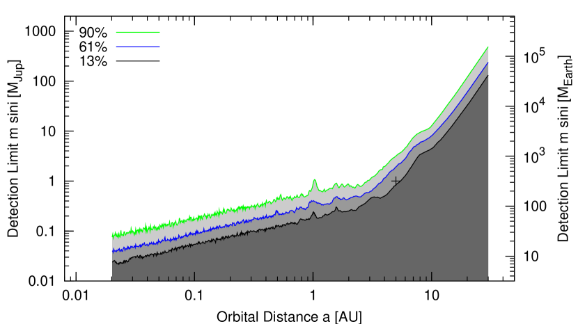
Figure 7: Sensitivity of the survey. For each orbital distance the minimum mass is indicated that could have been detected for 4, 19, and 28 stars of the 31 stars (corresponding to a fraction of 13%, 61%, and 90%) with 99.9% significance. The cross marks again a Jupiter analogue.

5 Discussion on individual targets

In this section we discuss individually those stars that exhibit variability.

$\beta$ Hyi:

For $\beta$ Hyi Endl et al. (2002) announced a trend of 7 m/s/yr with a remaining scatter of 19 m/s. Here the best common trend is only 1.79 m/s/yr depicted with a black solid line in Fig. 19 (plus the secular acceleration of 0.86 m/s). The scatter around the HARPS data decreases to only 2.3 m/s (see Table A). However, the trend increases the VLC scatter from 7.4 m/s to 9.0 m/s and the fitted LC-VLC offset departs by 2.2$\sigma$ (-17 m/s, Table A) from the measured offset. Thus, it is unclear whether the trend is steady

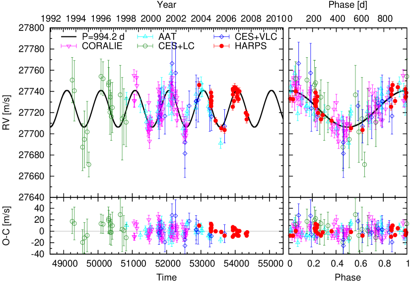
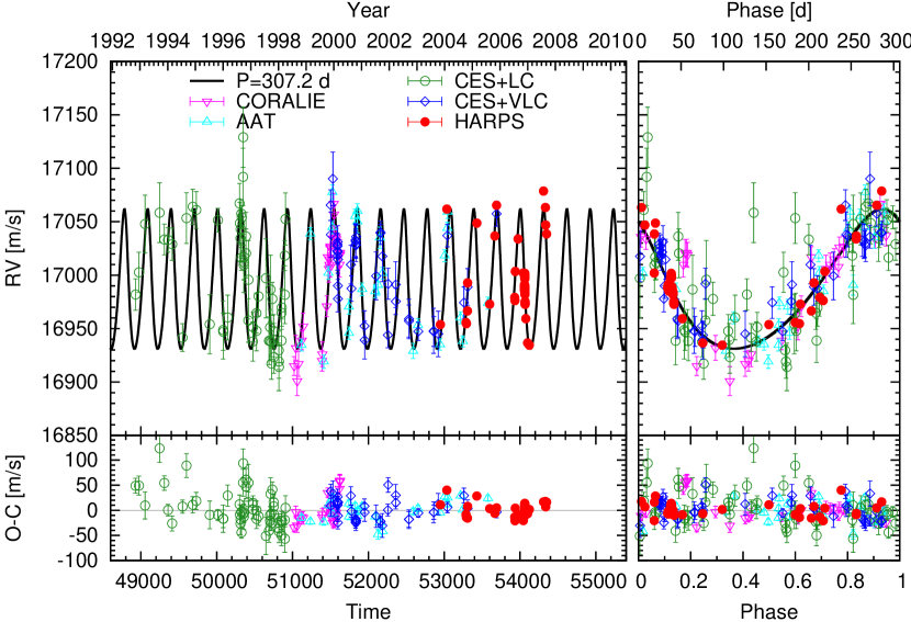
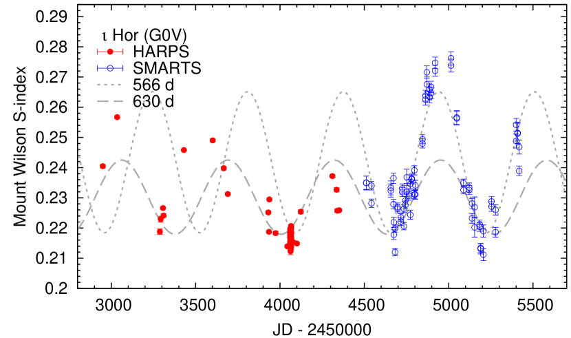
Additionally, we plot the 4300 d period tabulated for $\beta$ Hyi (Table 4.2) with a black dashed line in Fig. 19. This period matches that of a Jupiter analogue, while the amplitude of 6.5 m/s would result in a formal minimum mass of 0.56 $M_{\mathrm{Jup}}$. Compared to the trend in the previous section the fitted LC-VLC offset is less discrepant (-8.0 m/s), but the sine fit is less significant than trend and still not supported by the VLC data, because their scatter increases from 7.4 m/s to 8.9 m/s. Moreover, $\log R^{\prime}_{\mathrm{HK}}$ and FWHM correlate with the RVs. Hence the long-term variations might be related to the magnetic cycle. HR 209: $\log R^{\prime}_{\mathrm{HK}}$ and FWHM correlate with the RVs. Hence the RV variations are related to stellar activity probably induced by spots. HR 506 (HD 10647): A planet candidate was presented by Mayor et al.${}^{\text{\ref{fn:Mayor03}}}$ based on CORALIE measurements. Jones et al. (2004) found also weak evidence for a similar signal with the AAT, but did not exclude stellar activity as the cause. Butler et al. (2006) listed AAT RV data and derived orbital parameters. For HR 506 we clearly recovered the long RV period in the period analysis. Hence, we combine our observations with AAT data and CORALIE data to fit the orbit. Because more cycles have been covered, our combined solution gives a more precise period compared to the solutions given by the other authors ($P=(1003\,\pm\,56)$ d, $e=0.16\pm 0.22$ and $P=(1040\,\pm\,37)$ d, $e=0.18\,\pm\,0.08$, respectively). For our three combined data sets an eccentric orbit does not fit much better (Table 4.2) and also in the solution for the five combined data sets the eccentricity vanished. Therefore a circular obit was fitted ($e$ and $\omega$ fixed to zero, Table 6, Fig. 8). The semi-axis and the companion minimum-mass were derived by assuming a stellar mass of $1.17\pm 0.1\,M_{\oplus}$ (Table 2). Figure 8: Left: RV time series for HR 506 combined with AAT and CORALIE data. Right: RVs phase folded to the period of $P=995$ d and the residuals (bottom). Table 6: Orbital parameters for the planetary companion to HR 506. Parameter Value $P$ [d] 994.2 $\pm$ 8.6 $K$ [m/s] 17.3 $\pm$ 1.0 $T_{0}$ [JD] 2 450 088 $\pm$ 25 $\omega$ [^∘] 0 (fixed) $e$ 0 (fixed) $a$ [AU] 2.05 $\pm$ 0.24 $M\sin i$ [$M_{\mathrm{Jup}}$] 0.94 $\pm$ 0.05 $N$ 158 rms [m/s] 7.8 There is no clear RV-$\log R^{\prime}_{\mathrm{HK}}$ correlation ($r=0.45$, $\mathrm{FAP}=1.7\%$). However, when subtracting the 994 d RV period, there is a significant correlation ($r=0.63$, $\mathrm{FAP}=0.033\%$), implying that the residuals of this active star are affected by stellar activity. The RV-BIS and RV-FWHM correlations are not significant, also not for the residual RVs. The RV residuals of HR 506 also have some excess variability and a marginally significant trend of -2.41 m/s/yr which however increases the rms of the LC data (from 18.8 m/s to 20.0 m/s, Table A). $\tau$ Cet: The small trend reduces the scatter from 1.37 m/s to just 1.33 m/s and is just significant due to the large number of observations. However, at this level an instrumental cause is likely for the small trend and the RV-BIS and RV-FWHM correlation. In this respect we also like to point out that the FWHM of $\tau$ Cet (but also some others stars, e.g. $\zeta$ Tuc) exhibits a noticeable positive long-term trend (Fig. 31) which might be due to a drifting focus of HARPS. In this case, assuming a constant line equivalent width, a negative trend is expected and indeed seen in the contrast (depth) of the CCF (recently also noted by Gomes da Silva et al. 2012). $\tau$ Cet has the smallest variations in $\log R^{\prime}_{\mathrm{HK}}$ in the sample. $\kappa$ For: The RVs of $\kappa$ For decline over the whole time baseline of 14 yr which indicates an orbital period longer than the estimate of 21 yr given in Endl et al. (2002). The Keplerian period of 10700 d listed in Table 4.2 (29.3 yr) is not well constrained. However, again with the slope and Eq. (9) this period might be used to assess a minimum mass of 0.36 $M_{\odot}$ for the companion. The RV residuals do not exhibit significant variability. $\iota$ Hor: For this active star Kürster et al. (2000) discovered a planet. The signal was also seen by Naef et al. (2001) using the CORALIE spectrograph and by Butler et al. (2001) with the AAT. Using the HARPS data of Vauclair et al. (2008) taken for an asteroseismology campaign, Boisse et al. 2011 searched for short period companions ($P<7$ d), but detected no further planet. In our analysis we recovered the planetary signal seen for $\iota$ Hor by Kürster et al. (2000). We refined the orbital parameters with our data sets and included also the AAT (Butler et al. 2006) and CORALIE data (Naef et al. 2001) as shown in Fig. 9. For these two data sets the jitter estimate (from Table A) was added to the measurements error. Due to the activity of the star the residuals have a high scatter. The orbital parameters are listed in Table 7. The semi-axis and the companion minimum-mass were derived by assuming a stellar mass of $1.25\pm 0.02\,M_{\oplus}$ (Table 2). An astrometric upper mass limit of 18.4 $M_{\mathrm{Jup}}$ was placed by Reffert & Quirrenbach (2011) in combination with the orbital solution of Butler et al. (2006). The orbital period of 307 d is different from the rotation period of $\sim$8 d (see below), while a relation with the magnetic cycle has to be discussed. Metcalfe et al. (2010) reported that a magnetic activity cycle of $\sim$1.6 yr bears no obvious relation to the orbital period, but we find that there is a moderately significant RV-$\log R^{\prime}_{\mathrm{HK}}$ correlation (Fig. 33) and that the refined orbital period (307 d) is half of the formal best-fitting period (630 d) for the combined HARPS and SMARTS $S_{\mathrm{HK}}$-index measurements (Fig. 10; we use the $S_{\mathrm{HK}}$-index instead of $\log R^{\prime}_{\mathrm{HK}}$ for the comparison, since Metcalfe et al. (2010) published $S_{\mathrm{HK}}$-index measurements). However, if the 307 d RV period were be caused by a magnetic cycle, we would expect the same period for the $S_{\mathrm{HK}}$-index and a positive correlation with the BIS (Lovis et al. 2011), while there is a formal RV-BIS anti-correlation probably artificially induced by the short-term variations (Fig. 11). Therefore we tend to prefer the planet hypothesis as a more simple and likely explanation. Moreover, after subtracting the 307 d period, the correlation with $\log R^{\prime}_{\mathrm{HK}}$ remains and the anti-correlation with BIS increases and becomes more significant. Figure 9: (Left) RV time series for $\iota$ Hor combined with AAT and CORALIE data. (Right) RVs phase folded to the period of $P=307$ d and the residuals (bottom). Table 7: Orbital parameters for the planetary companion to $\iota$ Hor. Parameter Value $P$ [d] 307.2 $\pm$ 0.3 $K$ [m/s] 65.3 $\pm$ 2.2 $T_{0}$ [JD] 2 449 110 $\pm$ 9 $\omega$ [^∘] 35 $\pm$ 10 $e$ 0.18 $\pm$ 0.03 $a$ [AU] 0.96 $\pm$ 0.05 $M\sin i$ [$M_{\mathrm{Jup}}$] 2.48 $\pm$ 0.08 $N$ 205 rms [m/s] 14.5 The periodogram of the residuals for $\iota$ Hor (Fig. 12) shows power at periods of 5.7 d as well as 7.94 d and 8.45 d (also found by Boisse et al. 2011 based on HARPS RVs). The latter peak coincides with periodic variations (8.5 d) found in the $S_{\mathrm{HK}}$ index by Metcalfe et al. (2010), which therefore probably indicates the rotation of this star. The residual RVs anti-correlate with BIS which is indeed expected for rotating spots (Boisse et al. 2011). Figure 10: S-index measurements for $\iota$ Hor. Metcalfe et al. (2010) published the SMARTS data (blue open circles) and the 566 d period (dotted line). The formal best fit for the combined data set is 630  d (dashed line).

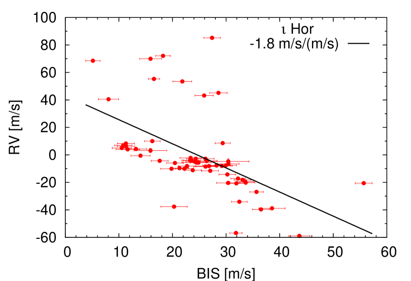
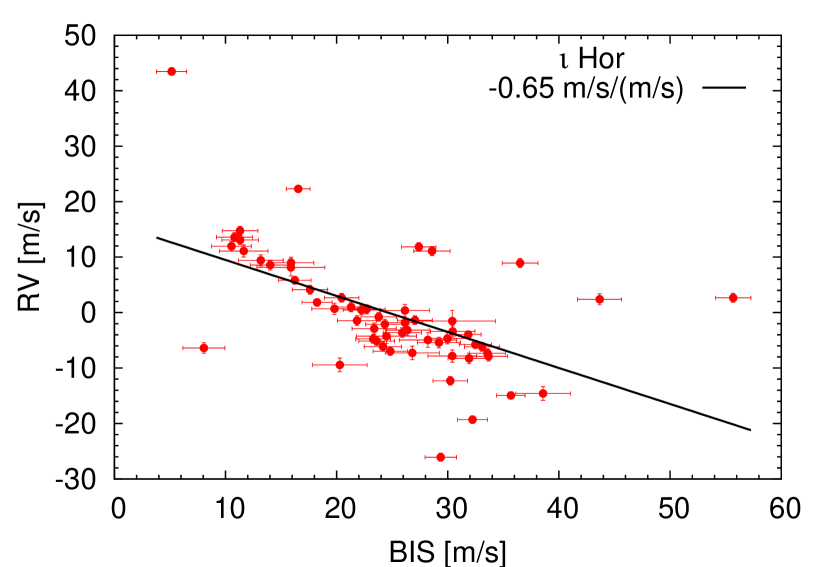
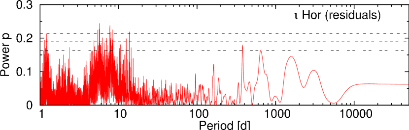
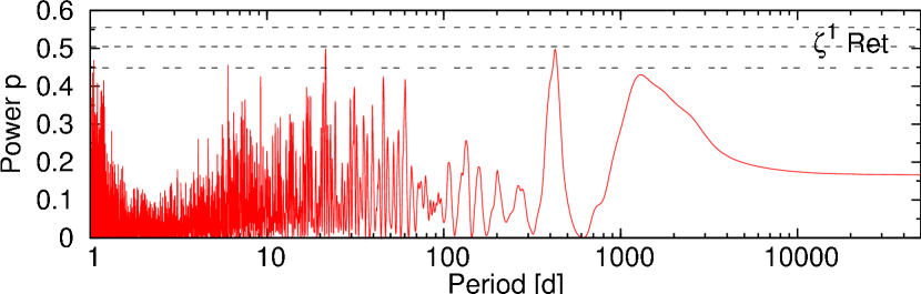
Figure 11: RV vs. BIS for $\iota$ Hor. (Top) The linear correlation coefficient is $r=-0.53$, but the correlation appears more complex and loop-like. (Bottom) After subtracting the 307 d period from the RVs, $r$ is $-0.56$. Figure 12: GLS periodogram on the residuals for $\iota$ Hor. In this and the subsequent figures (Figs. 13-15) the horizontal dashed lines depict FAP levels as in Fig. 5. $\alpha$ For: GJ 127 B can explain the trend of -11.5 m/s (Sect. 4.3, Table 5, Fig. 24). So far a trend is a sufficient model. The RV residuals do not exhibit significant variability. $\zeta^{1}$ Ret: The relatively large scatter of 12.5 m/s is indicative of excess variability and the periodogram of the RVs shows peaks close to our FAP threshold at 21.5 d and 426 d (Fig. 13) with the first giving the lowest for the combined rms value (but increasing the rms of the VLC data). The strong RV-$\log R^{\prime}_{\mathrm{HK}}$ (also RV-FWHM) correlation shows that most of the scatter is due to stellar activity, likely not only the magnetic cycle, since the observed correlation slope $219\pm 24$ m/s/dex exceeds the predicted value$140\pm 7$ m/s/dex the for a magnetic cycle (Sect. 4.5, assuming $5746\pm 27$ K and $\mathrm{[Fe/H]}=-0.22\pm 0.05$ from del Peloso et al. 2000). $r=0.88$ indicates that the subtraction of this correlation will reduce the scatter by $\sqrt{1-r^{2}}$ to 5.9 m/s. $\zeta^{1}$ Ret has the largest $\log R^{\prime}_{\mathrm{HK}}$-variations and a quite high jitter estimate of 3.8 m/s within our sample. Figure 13: GLS periodogram for $\zeta^{1}$ Ret. $\zeta^{2}$ Ret: Given the very similar stellar parameters of the binary pair $\zeta^{1}$ Ret and $\zeta^{2}$ Ret, del Peloso et al. (2000) already pointed out the baffling fact of their very different activity level. We do not find any significant RV excess variability for $\zeta^{2}$ Ret. However, there is a significant RV-FHWM correlation and all three activity indicators seem to exhibit a small trend, which might be either due to a magnetic cycle or instrumental (cf. $\tau$ Cet). $\epsilon$ Eri: Hatzes et al. (2000) announced a planet in an eccentric orbit ($e=0.6$) around this active star. Benedict et al. (2006) refined the orbital solution and combined the RVs with astrometric observations with the HST Fine Guidance Sensor indicating an orbital inclination of $i=30^{\circ}$. Likewise, Reffert & Quirrenbach (2011) derived a similar value for the inclination and an upper mass limit of 6.1 $M_{\mathrm{Jup}}$ using Hipparcos astrometry and the RV orbit solution. However, in the periodogram for $\epsilon$ Eri (Fig. 14) we cannot find any evidence for the long-period planet ($P$=2500 d) suggested by Hatzes et al. (2000) whose orbital solution is plotted in Fig. 20 for comparison. Due to the higher precision of our data, the combined rms is 8.2 m/s for fitting a constant, while Hatzes et al. (2000) list an rms ranging from 11 to 22 m/s for different instruments in the residuals of their Keplerian model. $\epsilon$ Eri is an active star and all three activity indicators are variable, and the BIS shows an anti-correlation with RV. The stellar rotation period is 11.2 d (Donahue et al. 1996; Fröhlich 2007). On a short time scale of 85 min its variability is 0.86 m/s (Table A), while the long term jitter estimate is 3.6 m/s (Table A). Our best-fitting sine function has a period of 3.11 d, reduces the scatter from 8.2 m/s to only 6.9 m/s, but is not significant. We note that, combining the RVs of HARPS and all the RVs given in Benedict et al. (2006), Anglada-Escudé & Butler (2012) could also not confirm the planet solution, though, without evaluating the significance, they suggested another best fitting, similar long-period.

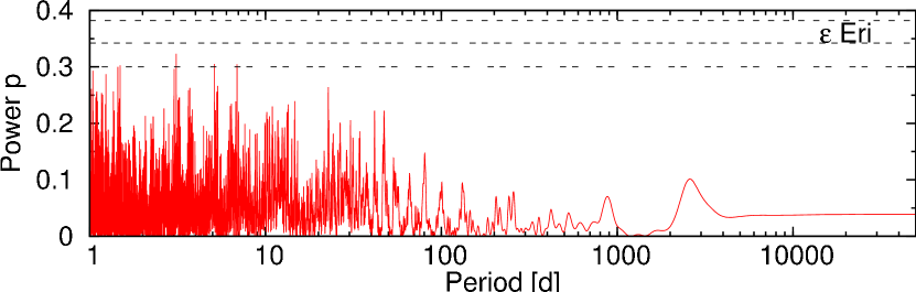
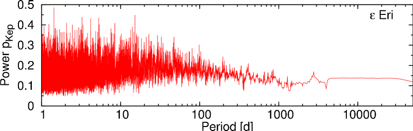
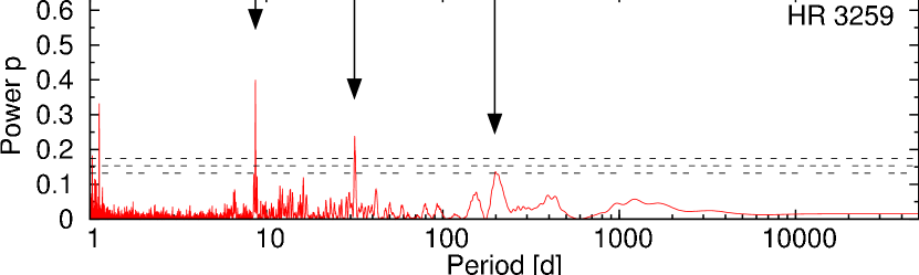
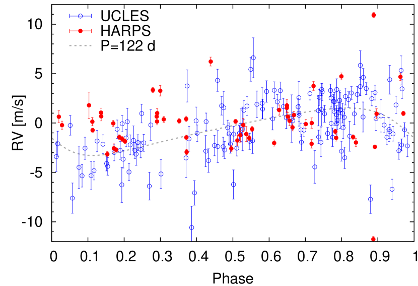
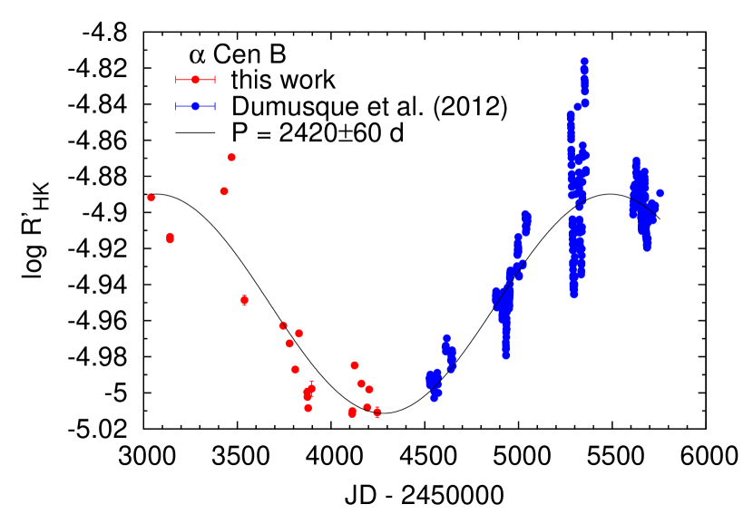
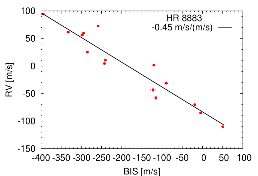
Figure 14: GLS (top) and Keplerian (bottom) periodogram for $\epsilon$ Eri. There is no significant power at the period of the putative planet $\epsilon$ Eri b ($P=2500$ d). $\alpha$ Men: Eggenberger et al. (2007) reported a companion for $\alpha$ Men which is likely an M3.5 – M6.5 dwarf that was seen at a separation of 3.05” with the VLT+NACO. They also mentioned (but did not quantify) a radial velocity drift for $\alpha$ Men seen with the CORALIE spectrograph and suggested that the companion causes this trend. In our data however, the star has no significant excess variability ($\mathrm{rms}=3.1$ m/s) or trend. Therefore we cannot confirm an RV trend for $\alpha$ Men, whose value should be unchanged over years if induced by an M dwarf with a separation of 3″. However, since no value for the trend was given by Eggenberger et al. (2007), a quantitative comparison cannot be made. Moreover, the RVs correlate with all three activity indicators. The observed RV-$\log R^{\prime}_{\mathrm{HK}}$ slope of $57\pm 10$ m/s/dex (Table A) agrees with the predicted sensitivity of $C_{RV}=69\pm 4$ m/s/dex (assuming $T_{\mathrm{eff}}=5594\pm 36$ K and $\mathrm{[Fe/H]}=0.10\pm 0.05$ from Santos et al. 2004) indicating a magnetic cycle as cause of the RV variations. HR 2400: The orbital solution for HR 2400 is given in Table 8. Assuming a stellar mass of $1.2\pm 0.1\,M_{\oplus}$ (Table 2) the companion has a minimum mass of 0.17 $M_{\mathrm{\odot}}$ indicating an M dwarf at a separation of 9.6 AU (0$\aas@@fstack{\prime\prime}$26). Hence, HR 2400 is a single-lined spectroscopic binary (SB1). Figure 24 displays the RV residuals for HR 2400 which do not have a significant variability. In the FWHM there seems to be a trend which might be due to stellar activity or spectral contamination by the companion. In the residuals the RV-FWHM correlation vanished. Table 8: Orbital parameters for the companion to HR 2400. Parameter Value $P$ [d] 9346 $\pm$ 554 $K$ [m/s] 1717 $\pm$ 83 $T_{0}$ [JD] 2 451 881 $\pm$ 16 $\omega$ [^∘] 279 $\pm$ 1 $e$ 0.58 $\pm$ 0.01 $a$ [AU] 9.6 $\pm$ 1.1 $M\sin i$ [$M_{\odot}$] 0.17 $\pm$ 0.01 $N$ 77 rms [m/s] 4.8 HR 3259: For HR 3259 Lovis et al. (2006) reported a planetary system with three Neptune-mass planets with periods (amplitudes) of 8.667 d (3.51 m/s), 31.56 d (2.66 m/s), and 197 d (2.20 m/s). All three periods are seen in the periodogram (Fig. 15) and the corresponding peak heights are in the same order as suggested by the given amplitudes. We refer to Anglada-Escudé & Butler (2012) for a recent and detailed analysis of the HARPS data and updated orbital parameters of the short period planets. We only note that with our own and archive (but without GTO) HARPS data alone we also have seen excess power at these periods, although these peaks did not reach our FAP threshold due to too few observations (only 18 binned HARPS data points) and considerable spectral leakage (aliasing). Figure 15: GLS periodogram for HR 3259. The vertical arrows indicate the periods for the three planets announced by Lovis et al. (2006). HR 3677: The orbit of the companion to the giant HR 3677 is eccentric indicated by the much lower residuals when fitting a Keplerian orbit (8.7 m/s) compared to a circular orbit (35 m/s). Using the slope and Eq. (9) a raw estimate for the minimum companion mass is 0.69 $M_{\odot}$. The significant excess variability of the RV residuals (Fig. 24) is likely explained by an underestimated jitter of this giant. The RV-FWHM correlation disappears in the residuals. HR 4523: Tinney et al. (2011) reported a Neptune-like planet with 16 $M_{\oplus}$ minimum mass in a 122 d orbit. However, the periodogram of our data shows no power at periods of 122 d. Therefore we cannot confirm the planet reported by Tinney et al. (2011). Their 145 measurements over 7 yr with UCLES have a scatter of $\mathrm{rms}=3.0$ m/s. For comparison, the 62 HARPS RVs over 4.4 yr have also $\mathrm{rms}=2.9$ m/s. Figure 16 shows the RV data phase folded to the period of the proposed planet. When subtracting the proposed orbital solution, the scatter decreases to 2.56 m/s for UCLES, but increases to 3.29 m/s for HARPS. Figure 16: RV data for HR 4523 phase folded to 122.1 d. The dashed curve is an orbital solution proposed by Tinney et al. (2011) based on the UCLES data. HARPS RVs are shown for comparison. HR 4979: Most of the RV variations is likely caused by a magnetic cycle, because the RV correlates with $\log R^{\prime}_{\mathrm{HK}}$ and BIS. Moreover, the observed correlation slope is $81\pm 12$ m/s/dex which is of the order of the value expected for magnetic cycles ($65\pm 2$ m/s/dex; Sect. 4.5, assuming $T_{\mathrm{eff}}=5729\pm 17$ K and $\mathrm{[Fe/H]}=0.19\pm 0.01$ from Sousa et al. 2008). $\alpha$ Cen A+B: We refer to Pourbaix et al. (2002) for the orbital solution for $\alpha$ Cen A+B with a period of 80 yr. We would just like to point out that the fitted trends in Sect. 4.3, although obviously not a sufficient model, can be interpreted as a mean acceleration and that the ratio of these slopes is a measure of the mass ratio $\frac{M_{\mathrm{A}}}{M_{\mathrm{B}}}=-\frac{\dot{RV}_{\mathrm{B}}}{\dot{RV}_{\mathrm{A}}}=\frac{154.4\,\mathrm{m/s/yr}}{130.9\,\mathrm{m/s/yr}}=1.180$ which agrees with the value of $\frac{M_{\mathrm{A}}}{M_{\mathrm{B}}}=\frac{1.105\,M_{\odot}}{0.934\,M_{\odot}}=1.183$ derived from Pourbaix et al. (2002). Neither the residuals of $\alpha$ Cen A nor $\alpha$ Cen B exhibit a significant variability. However, using HARPS measurements and a very complex analysis, Dumusque et al. (2012) have recently announced a planet candidate for $\alpha$ Cen B with a very small amplitude (0.51 m/s, 3.236 d). Due to the lower number of the (complementary) HARPS measurements in this work (21 vs. 459) we are not sensitive to this planet. The RV-$\log R^{\prime}_{\mathrm{HK}}$ and RV-BIS correlations listed for $\alpha$ Cen B are only formally significant, since obviously the RV trend is caused by $\alpha$ Cen A and not by a stellar activity, and vanishes after subtracting the orbit. The trend seen in $\log R^{\prime}_{\mathrm{HK}}$ is part of a longer magnetic cycle which be seen more clearly when adding recently published HARPS data by Dumusque et al. (2012). We estimate a period of $P\sim 2420$ d (Fig. 17) for the magnetic cycle, but a true periodicity is not secured, since only one cycle is covered and e.g. Buccino & Mauas (2008) reported a period of 3061 d with a FAP of 24%. Figure 17: The time behaviour of $\log R^{\prime}_{\mathrm{HK}}$ that shows the magnetic cycle of $\alpha$ Cen B. GJ 570 A: The trend has a smaller FAP compared to sinusoidal and Keplerian model and is therefore a sufficient model for the RV. GJ 570 BC can explain the trend of -2.7 m/s (Sect. 4.3, Table 5). Also, there is a marginally significant linear correlation of the RVs with BIS and FWHM and therefore stellar activity could contribute to the trend as well. HR 6416: GJ 666 B can explain the trend of 9.4 m/s (Sect. 4.3, Table 5). A trend is a sufficient model. The residuals do not exhibit significant excess variability. HR 7703: A trend is a sufficient model and the value of 3.6 m/s (Sect. 4.3, Table 5) can be explained by GJ 783 B. Therefore the formally significant RV-$\log R^{\prime}_{\mathrm{HK}}$correlation should be artificial, however an additional (positive or negative) contribution to the trend by activity cannot be excluded. After removing the trend, there is no significant correlation or excess variability. HR 8323: The listed significant period of 1372 d is caused by a stellar magnetic cycle. All three activity indicators show similar variations and strong correlations with RVs (Fig. 54, Table A and A). The observed slope of $98\pm 10$ m/s/dex (Table A) agrees well with the predicted RV-$\log R^{\prime}_{\mathrm{HK}}$ sensitivity of $C_{RV}=108\pm 2$ m/s/dex for a magnetic cycle (assuming $T_{\mathrm{eff}}=5937\pm 13$ K and $\mathrm{[Fe/H]}=0.00\pm 0.01$ from Sousa et al. 2008). $\epsilon$ Ind A: The trend for $\epsilon$ Ind A originally announced by Endl et al. (2002) is probably of highest interest, since it might be caused by a planet. The wide binary brown dwarf companion $\epsilon$ Ind B ($M_{Ba}+M_{Bb}=112\,M_{\mathrm{Jup}}$, King et al. 2010) is too far from $\epsilon$ Ind A (Table 5, Sect 4.3). It can induce only an acceleration of 0.009 m/s/yr and hence cannot explain the measured trend. The common slope of 2.4 m/s/yr is predominantly based on the more precise HARPS data. This trend improves the individual rms of the LC and VLC only slightly (see Table A), however the rms for both data sets is close to or below the stated precision. The scatter of the VLC data around the trend is even only 4.4 m/s, making it the most precise star in the VLC data set. In the overall picture the trend seems to be present for the whole observation. The fit places the offset between LC and VLC at -4.0 m/s (Table A, visible as the small jump in the fit in Fig. 23, $\eta=0.52$), i.e. is consistent with our physically estimated offset. With in our sample, $\epsilon$ Ind A exhibits comparably large variations in $\log R^{\prime}_{\mathrm{HK}}$ ($\mathrm{rms}_{\mathrm{RHK}}=0.032$ dex, Table A). Since both the RVs and $\log R^{\prime}_{\mathrm{HK}}$ (as well as FWHM) values have a long-term trend during the HARPS observations (Fig. 55), this results in a significant correlation ($r=0.60$). However, both trends could coincide just by chance temporarily, so that it is still not clear whether they are associated with the same long-term period (if any). Note also that the last $\log R^{\prime}_{\mathrm{HK}}$ observations seem to depart from a steady trend in contrast to the RVs. HR 8501: A trend is a sufficient model and GJ 853 B can explain its value of 17.3 m/s (Sect. 4.3, Table 5). The RV-BIS correlation should be artificial and vanishes in the residuals which also do not exhibit significant variability. HR 8883: The period of 7.6 d found for the giant HR 8883 improves only the HARPS rms, but not the LC and VLC rms (Table A). Endl et al. (2002) found strong Ca II H&K emission in a FEROS spectrum (cf. $S_{\mathrm{HK}}=0.533$ in Table A) and mentioned the high X-ray luminosity. Furthermore, the star is indicated in the Hipparcos catalogue (Perryman et al. 1997) as a photometrically variable star (variability flag ’U’, i.e. unresolved variable, e.g. irregular or semi-irregular variables). Finally, the large variation of the bisector span and the striking anti-correlation ($r=-0.96$) with the RVs as seen in the HARPS data (Fig. 18) reveal that the variations and periods of this star are intrinsic to the giant (e.g. rotation, activity, or solar-like oscillations). The RVs do not correlate with $\log R^{\prime}_{\mathrm{HK}}$ or FWHM (Table A and A, Fig. 57). Figure 18: Correlation between bisector span (BIS) and RV for the giant HR 8883.

6 Summary and Conclusion

Our sample consists of three planet hosting stars. These planets are already known and we are able to trace their periodic RV signals allowing confirmation of their reality. The planet hosting stars are $\iota$ Hor, discovered by this survey (Kürster et al. 2000), as well as HR 506 (Mayor et al.${}^{\text{\ref{fn:Mayor03}}}$) and HR 3259 (Lovis et al. 2006) which even has a system of three planets. However, we have no clear additional planet detection in our sample, while some promising or controversial cases like $\beta$ Hyi, $\epsilon$ Ind A, or $\epsilon$ Eri call for follow-up observations. Compared to our previous results in Endl et al. (2002), we confirm that: • $\kappa$ For, HR 2400, and HR 3677 are SB1 spectroscopic binaries with long periods. • $\alpha$ For, HR 6416, and HR 8501 exhibits trends consistent with their wide stellar companions. • $\epsilon$ Ind A has a steady long-term trend still explained by a planetary companion. Moreover, we see trends in HR 7703 and GJ 570 A which can also be explained by the known wide stellar companions listed in Table 5. However, the RV trend of $7$ m/s/yr reported for $\beta$ Hyi (Endl et al. 2002) is only 1.8 m/s/yr in the combined data set and is not seen in the VLC data. We cannot confirm a linear drift reported by Eggenberger et al. (2007) for $\alpha$ Men, neither can we confirm the planet HR 4523 b announced by Tinney et al. (2011), nor the planet $\epsilon$ Eri b reported by Hatzes et al. (2000). For $\epsilon$ Eri b, the astrometric results (Benedict et al. 2006; Reffert & Quirrenbach 2011) seem to confirm the planet, but they do not constitute independent detections, since they rely on the combination with less precise RV measurements. Also the astrometric phase coverage is not complete. However, the same is true for our HARPS measurements. Hence, this planet is not yet fully disproved with our RV non-detection or by imaging non-detections (e.g. Janson et al. 2007, 2008). Furthermore, there are also discussions whether an observed inner disk of warm dust can coexist with this inner planet (Reidemeister et al. 2011). It has to be pointed out that stellar magnetic cycles (the solar cycle length is 2$\times$ 11 yr) may cause long-term RV variations which might be mistaken as companions. The CaII H&K lines are an appropriate indicator to check this (Santos et al. 2010; Dumusque et al. 2011a; Lovis et al. 2011). Indeed, some stars, like e.g. HR 209, $\zeta^{1}$ Ret, and HR 8323 exhibit clear RV-$\log R^{\prime}_{\mathrm{HK}}$ correlations which originates from stellar activity and prevented us from claiming planets from the RV variations/periods. Hence, also in the search for Jupiter analouges, it is important to monitor activity indicators. Unfortunately, only the 4–5 yr of HARPS data contain the CaII H&K lines, so that the whole time baseline is not covered, which would have been especially desirable for HR 506 and $\iota$ Hor. We have not detected a Jupiter analogue, while our upper mass limits demonstrate that we are sensitive to Jupiter-mass planets up to 5 AU, i.e. Jupiter analogues (Fig. 7). In our sample the planet candidate with the longest period is HR 506 b (2.7 yr). While it has a minimum mass of one Jupiter mass, its period is still 4 times shorter than that of Jupiter. Although our sample size is too small to provide a meaningful number for the occurrence rate of Jupiters and Jupiter analogues, the two Jupiter-mass planets in our sample imply that our results are in agreement with the planet frequency of other much larger surveys. For example, from the ELODIE survey Naef et al. (2005) estimated a fraction of $7.5\pm 1.5$ % for stars hosting giant planets with periods less than 10 yr, while Cumming et al. (2008) derived a frequency of $12\pm 1.6$ % from the Keck survey and Mayor et al. (2011) $9.7\pm 1.3$ % (for $>100\,M_{\oplus}$) from the HARPS/CORALIE survey. For Jupiter analogs, i.e. only in the range of 3–6 AU, Lineweaver & Grether (2003) estimated a frequency of 5$\pm$2 % which is e.g. consistent with the discovery rate in the AAPS survey (3.3$\pm$1.4 %, Wittenmyer et al. 2011). Such low observed frequencies are compatible with the non-detection of a Jupiter analogue in our sample and a decreasing frequency of giant planets at larger distances ($\gtrsim 5$ AU) is also predicted with core accretion theory (Mordasini et al. 2012). The main reason for the limited VLC precision of $\sim$9 m/s is the short wavelength coverage of only 39 Å. Useful iodine lines cover a total wavelength range of 1000 Å. If this 25 time larger range could have been used, the extrapolated VLC precision would be 5 times higher, i.e. 1.8 m/s. The actively stabilised HARPS spectrograph has a larger wavelength coverage and an outperforming precision. The higher resolution of the CES+VLC is not necessarily an advantage because the stellar lines are nearly resolved already at the lower resolution of HARPS, i.e. they become not sharper and therefore do not provide much more RV information. Nevertheless the CES data are valuable for extending the time baseline to 15 years. The problem of combining long-term precision RV data from different instruments complicates the analysis. We could derive the zero point offset between LC and VLC only with a limited precision which leads to a loss of sensitivity for trends and long periods. However, this problem can occur in long-term surveys quite frequently as spectrographs receive upgrades or survey projects are transferred to new instruments. Long-term access to the same instrument/instrument configuration is therefore important. While the RV method probes the inner region of the stellar environment, the outer regions can be explored for planets with direct imaging. Since both methods complement each other, their combination leads to a more complete picture about the existence and nature of planets around stars. An example is $\epsilon$ Ind A, where despite the high imaging sensitivity with HST/NICMOS and VLT/NACO (Geißler et al. 2007; Janson et al. 2009) the non-detection puts constraints to the companion which induces the observed RV trend of 2.4 m/s/yr. Hence the results and detection limits from our survey can be valuable for other campaigns which target these bright stars. Some of our nearby and bright stars are also the subject of projects searching and studying surrounding debris disks. Structures in these disks permit conclusions about the presence of outer planets. For example, the Herschel satellite has resolved exo-Kuiper belts around $\zeta^{2}$ Ret (Eiroa et al. 2010) and around HR 506 (q¹ Eri, Liseau et al. 2010). In the case of the RV planet-hosting star HR 506, the structure of a ring at 35-40 AU provides a hint for another planet. Similarly, the structure of the known debris disk of $\epsilon$ Eri suggests an outer planet (Quillen & Thorndike 2002). But then for HR 8501 that has an RV trend likely due to its wide stellar companion, Eiroa et al. (2010) exclude a cold debris disk.

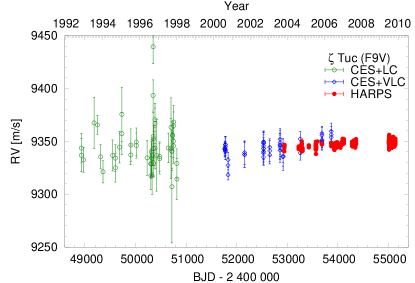
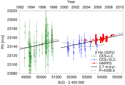
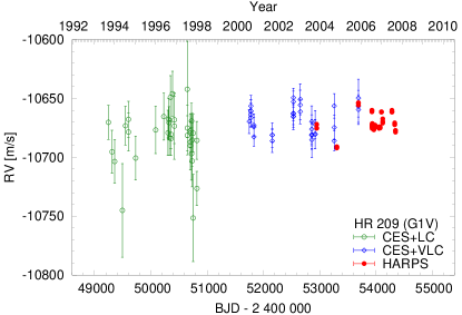
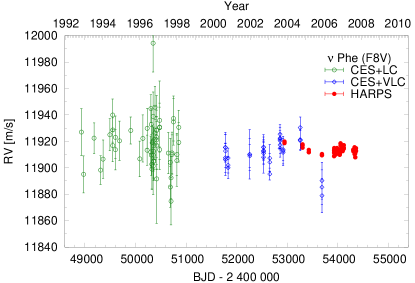
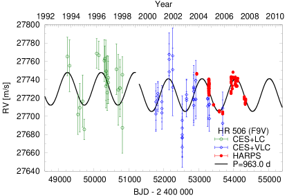
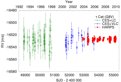
Figure 19: Radial velocity time series (unbinned data). The error bars depict the internal measurement errors $\Delta RV_{i}$, i.e. not including jitter. LC (green open circles) and VLC (blue open diamonds) data are displayed with their measured offsets. Jumps in the curves indicates the difference between the measured (Sect. 3.5) and fitted (Sect. 4) LC-VLC offset. HARPS data are in red filled circles. The solid lines indicate significant models, while dashed lines illustrate less or non-significant alternative models. All models include secular acceleration. Model curves are shown for $\beta$ Hyi (trend and long-period sinusoid, see text for discussion), and HR 506 (sinusoid).

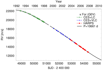
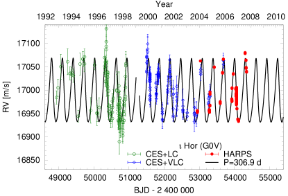
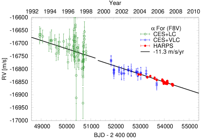
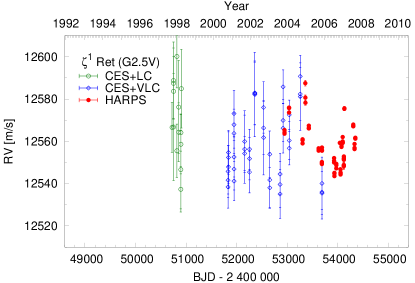
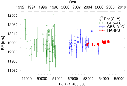
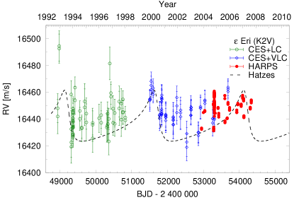
Figure 20: Radial velocities. Continuation of Fig. 19. Model curves are shown for $\kappa$ For (Keplerian), $\iota$ Hor (Keplerian), and $\alpha$ For (trend). The Keplerian orbit for $\epsilon$ Eri taken from Hatzes et al. (2000) is not significant in this work.

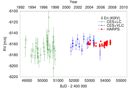
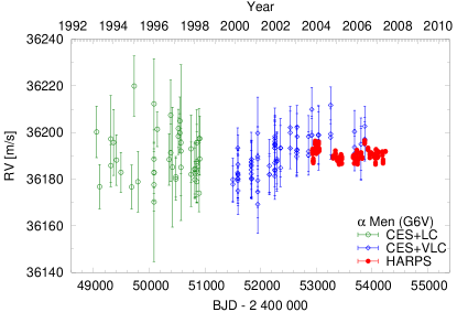
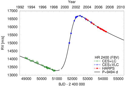
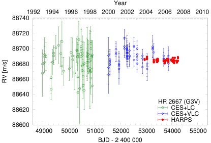
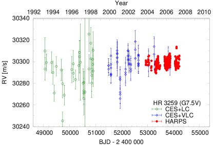
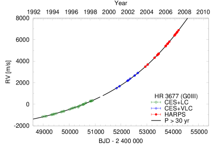
Figure 21: Radial velocities. Continuation of Figs. 19 and 20. Model curves are shown for HR 2400 (Keplerian) and HR 3677 (Keplerian).

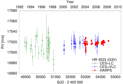
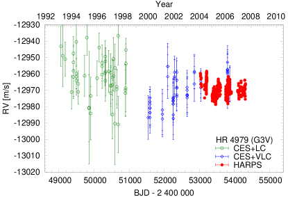
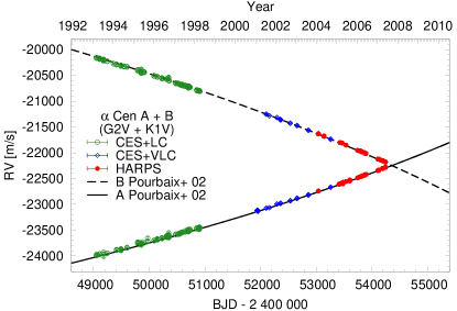
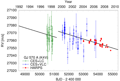
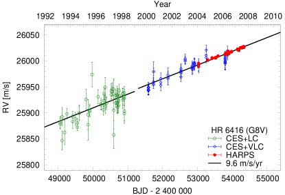
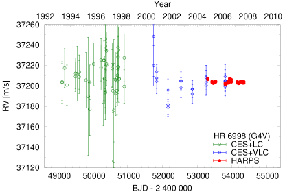
Figure 22: Radial velocities. Continuation of Figs. 19–21. Model curves are shown for $\alpha$ Cen A and $\alpha$ Cen B (Keplerian orbit from Pourbaix et al. 2002), GJ 570 A (trend), and HR 6416 (trend).

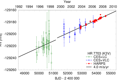
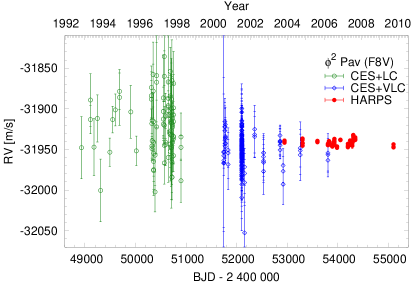
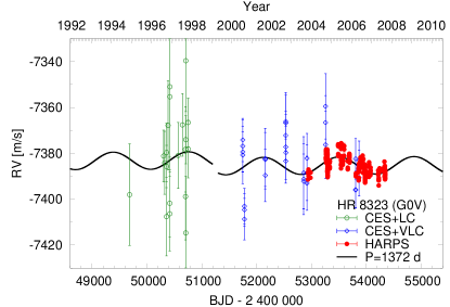
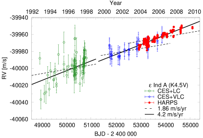
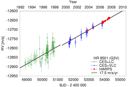
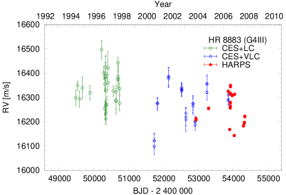
Figure 23: Radial velocities. Continuation of Figs. 19–22. Model curves are shown for HR 7703 (trend), HR 8323 (sinusoid), $\epsilon$ Ind A (constant, i.e. only secular acceleration of 1.86 m/s/yr, and trend), and HR 8501 (trend).

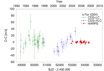
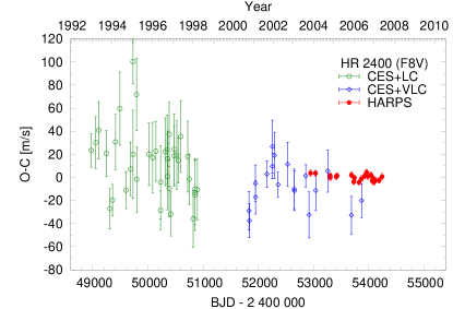
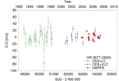
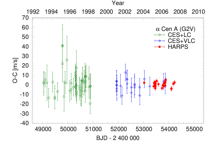
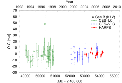
Figure 24: Residual RVs (binned as described in Sect. 4) for the spectroscopic binaries.

Appendix A Accompanying Tables

Table 9: Residual rms detailed for each instrument resulting from the joint analysis for fitting a constant, slope, sinusoid, and Keplerian orbit.

Table 10: Jitter estimation. $\sigma_{\mathrm{jit},\tau}$ is the weighted${}^{\text{\ref{fn:binweight}}}$ scatter of the HARPS data in the 2 h bins and $\tau$ is the weighted${}^{\ref{fn:bintime}}$ mean of the time coverage in these bins (which may not cover the real jitter time scales in all cases). $\log R^{\prime}_{\mathrm{HK}}$ and activity index $S_{\mathrm{HK}}$ are median values from the HARPS data of this work. The jitter estimation on long time scales $\sigma_{\mathrm{jit,long}}$ was derived as described in Isaacson & Fischer (2010) using B-V (Perryman et al. 1997) and $S_{\mathrm{HK}}$ (this work). For comparison some literature $S_{\mathrm{HK}}$ values are given ([H] Henry et al. 1996, [G] Gray et al. 2006, [W] Wright et al. 2004) and the jitter $\sigma_{\mathrm{jit,IF10}}$ (“quadrature difference of velocity rms minus the formal internal errors”) as given by Isaacson & Fischer (2010) for stars monitored with Keck.

Table 11: Offset differences $c_{\mathrm{VLC}}-c_{\mathrm{LC}}$ [m/s] in the fits. For a reasonable model the expected value for the offset difference is zero with an uncertainty of $\sim 8$ m/s (Sect. 3.5).

Table 12: Correlations of RV with $\log R^{\prime}_{\mathrm{HK}}$ and BIS for the HARPS data. Listed for both are the mean, the rms, the slope, the correlation coefficient $r$ and its false alarm probability. Significant correlation coefficients with $\mathrm{FAP}<0.01$ are in bold font.

Table 13: Correlations of RV with FWHM for the HARPS data. Listed are the mean, the rms, the slope, the correlation coefficient $r$ and its false alarm probability. Significant correlation coefficients with $\mathrm{FAP}<0.01$ are in bold font.

Appendix B Online figures: HARPS time series and Correlation plots for RVs, $\log R^{\prime}_{\mathrm{HK}}$ and BIS

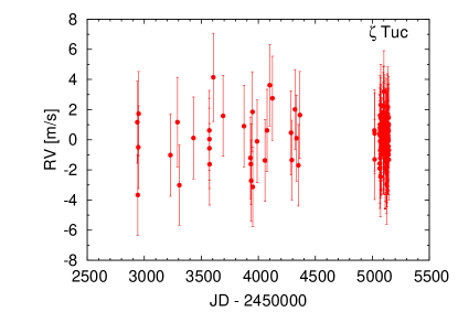
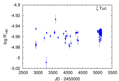
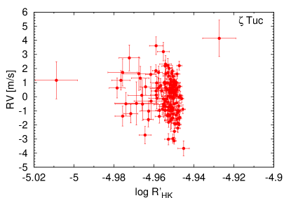
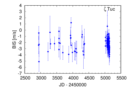
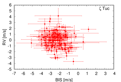
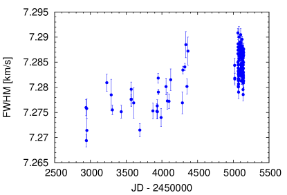
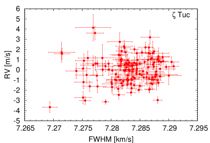
Figure 25: Activity indictors and correlations with HARPS RVs for $\zeta$ Tuc (2 h binned data, secular acceleration substracted, see Sect. 4.1).

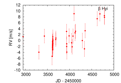
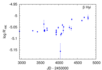
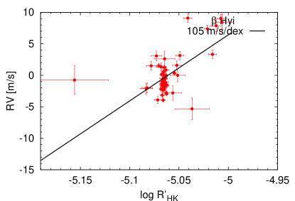
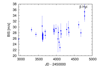
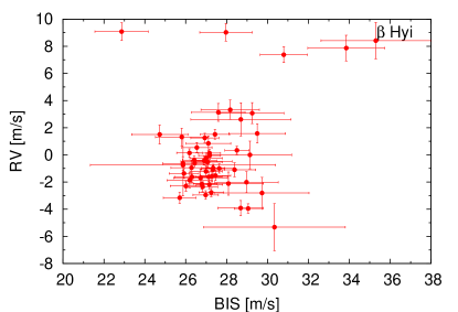
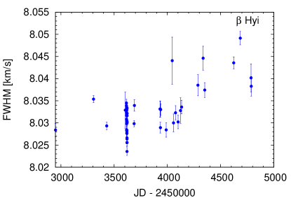
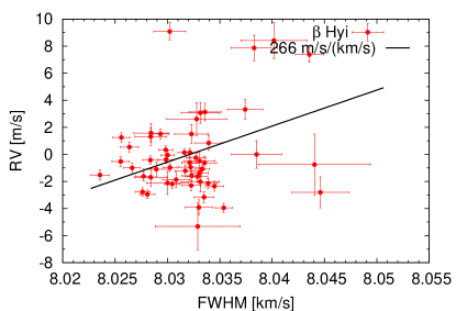
Figure 26: Activity indictors and correlations with HARPS RVs for $\beta$ Hyi (2 h binned data, secular acceleration substracted, see Sect. 4.1).

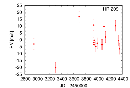
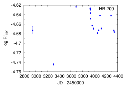
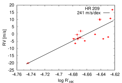
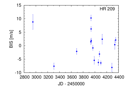
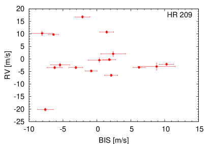
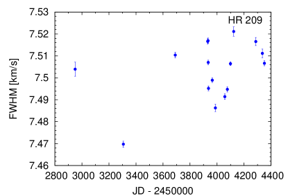
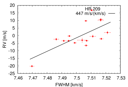
Figure 27: Activity indictors and correlations with HARPS RVs for HR 209 (2 h binned data, secular acceleration substracted, see Sect. 4.1).

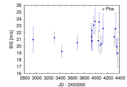
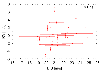
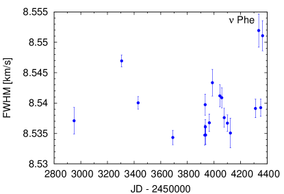
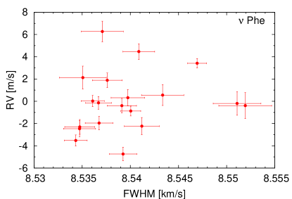
Figure 28: Activity indictors and correlations with HARPS RVs for $\nu$ Phe (2 h binned data, secular acceleration substracted, see Sect. 4.1).

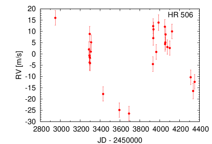
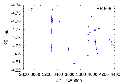
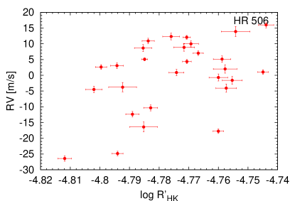
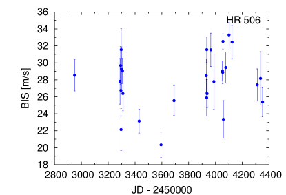
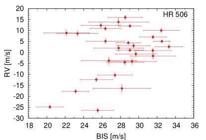
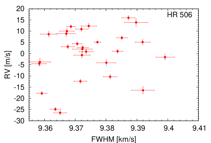
Figure 29: Activity indictors and correlations with HARPS RVs for HR 506 (2 h binned data, secular acceleration substracted, see Sect. 4.1).

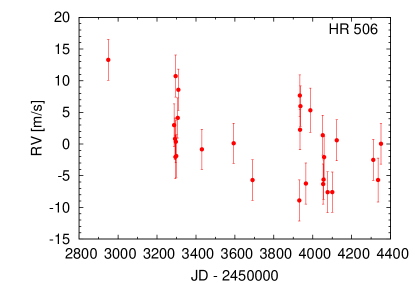
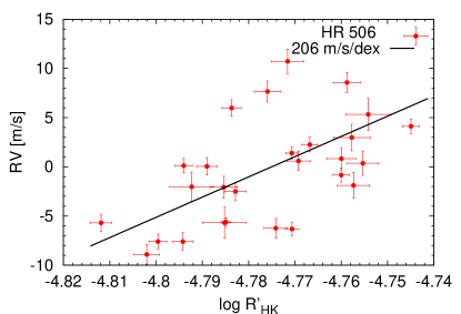
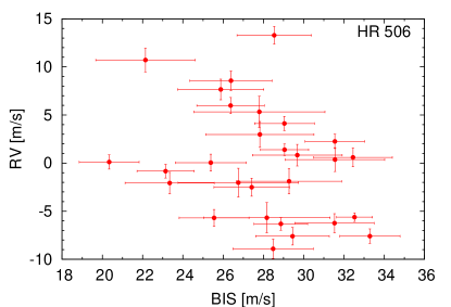
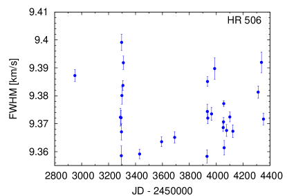
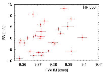
Figure 30: Activity indictors and correlations with HARPS RVs for the HR 506 residuals (2 h binned data, secular acceleration substracted, see Sect. 4.1).

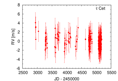
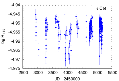
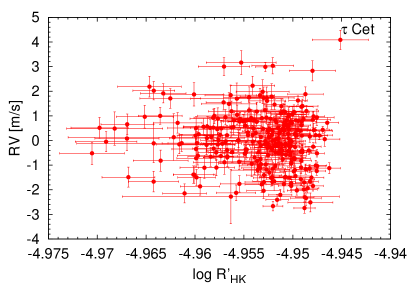
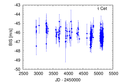
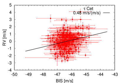
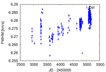
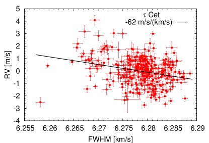
Figure 31: Activity indictors and correlations with HARPS RVs for $\tau$ Cet (2 h binned data, secular acceleration substracted, see Sect. 4.1).

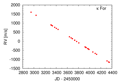
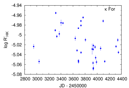
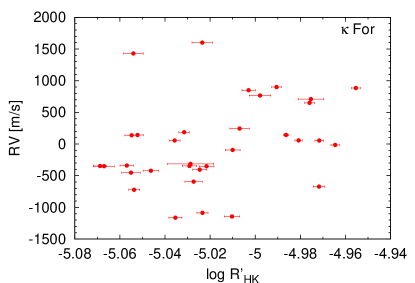
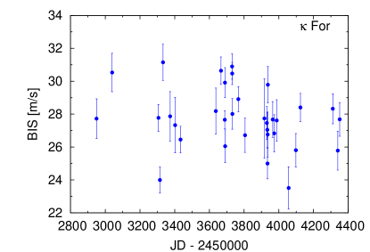
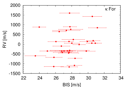
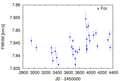
Figure 32: Activity indictors and correlations with HARPS RVs for $\kappa$ For (2 h binned data, secular acceleration substracted, see Sect. 4.1).

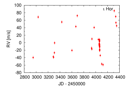
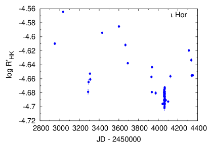
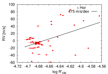
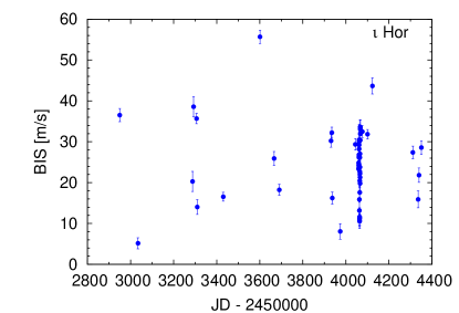
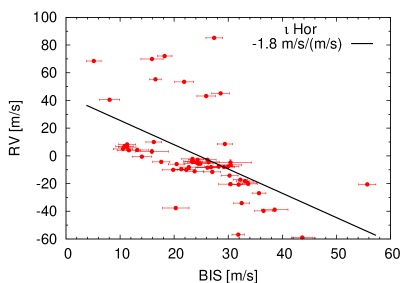
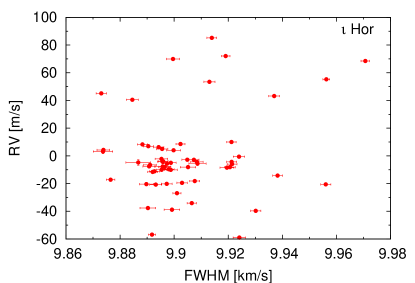
Figure 33: Activity indictors and correlations with HARPS RVs for $\iota$ Hor (2 h binned data, secular acceleration substracted, see Sect. 4.1).

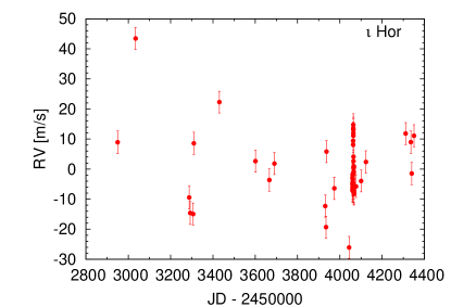
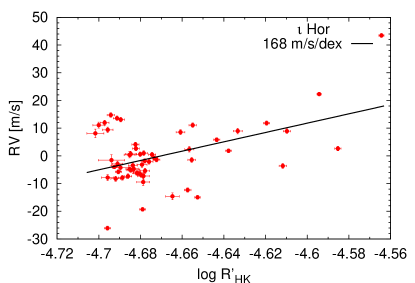
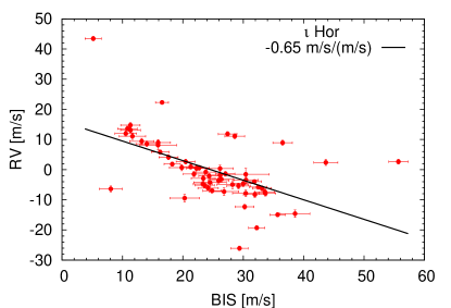
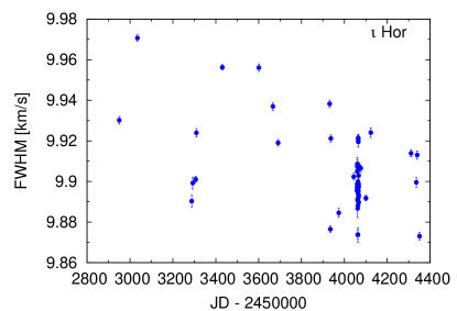
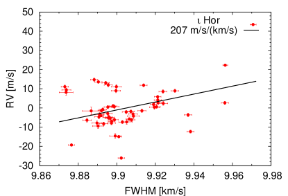
Figure 34: Activity indictors and correlations with HARPS RVs for the $\iota$ Hor residuals (2 h binned data, secular acceleration substracted, see Sect. 4.1).

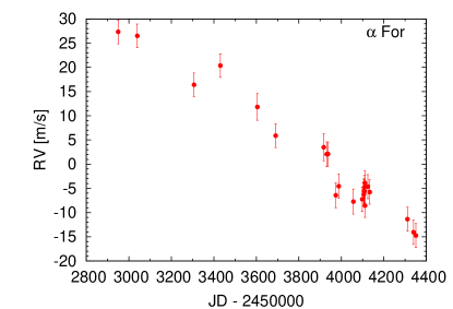
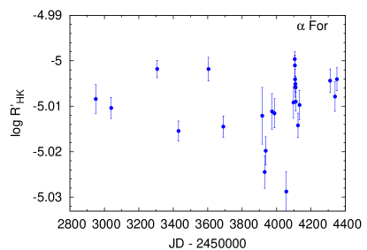
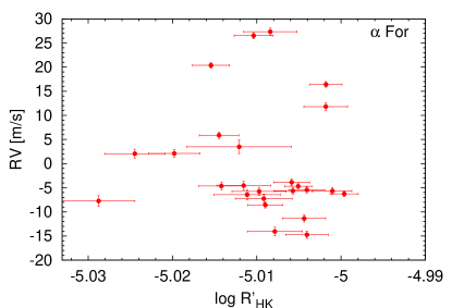
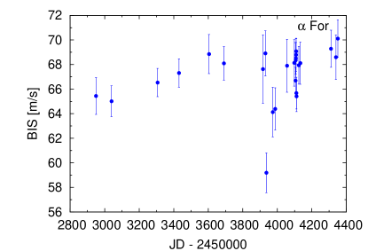
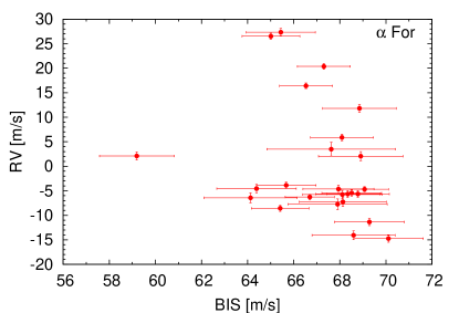
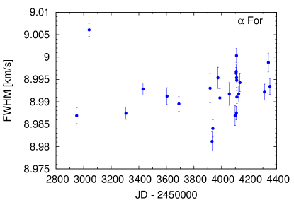
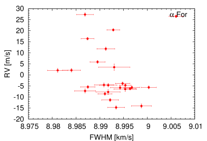
Figure 35: Activity indictors and correlations with HARPS RVs for $\alpha$ For (2 h binned data, secular acceleration substracted, see Sect. 4.1).

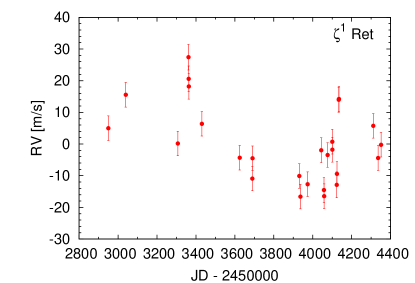
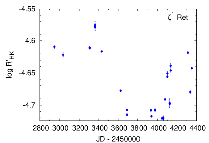
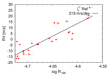
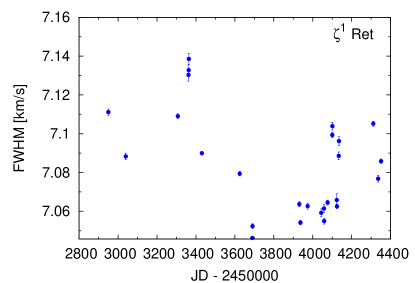
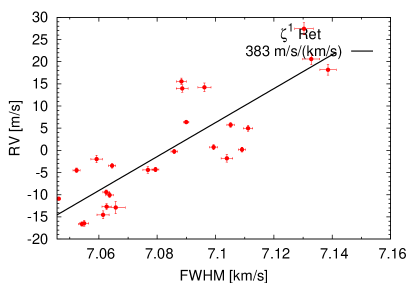
Figure 36: Activity indictors and correlations with HARPS RVs for $\zeta^{1}$ Ret (2 h binned data, secular acceleration substracted, see Sect. 4.1).

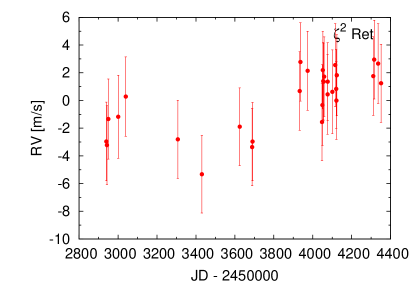
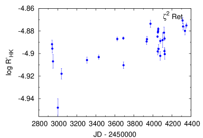
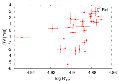
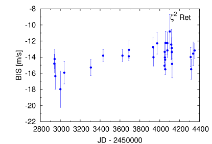
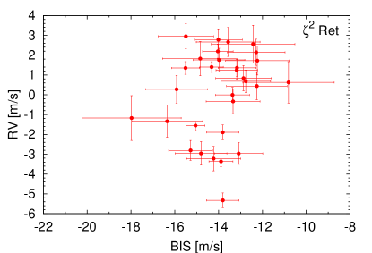
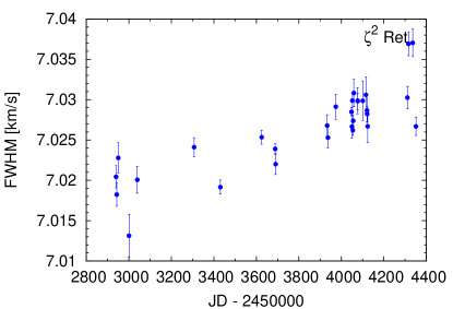
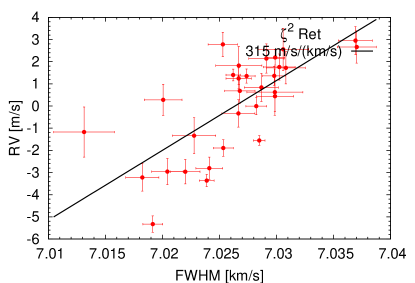
Figure 37: Activity indictors and correlations with HARPS RVs for $\zeta^{2}$ Ret (2 h binned data, secular acceleration substracted, see Sect. 4.1).

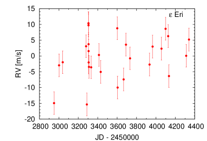
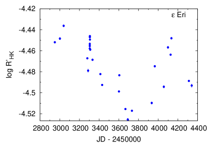
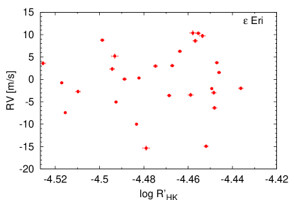
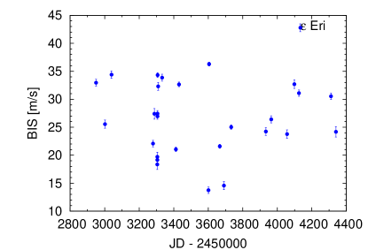
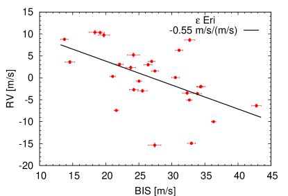
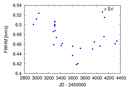
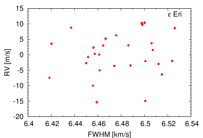
Figure 38: Activity indictors and correlations with HARPS RVs for $\epsilon$ Eri (2 h binned data, secular acceleration substracted, see Sect. 4.1).

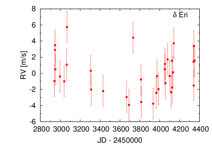
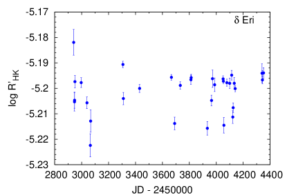
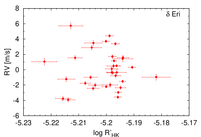
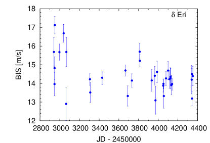
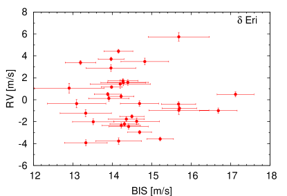
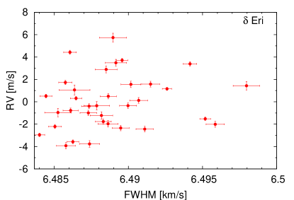
Figure 39: Activity indictors and correlations with HARPS RVs for $\delta$ Eri (2 h binned data, secular acceleration substracted, see Sect. 4.1).

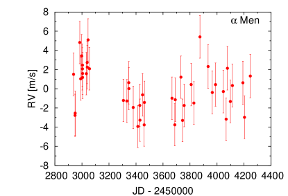
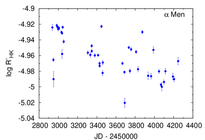
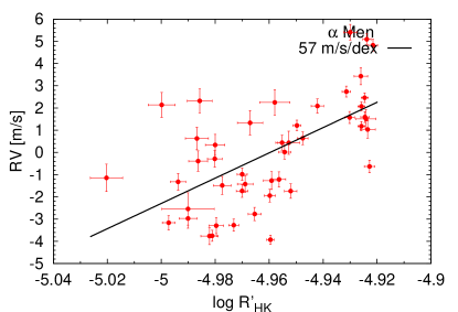
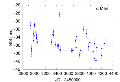
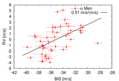
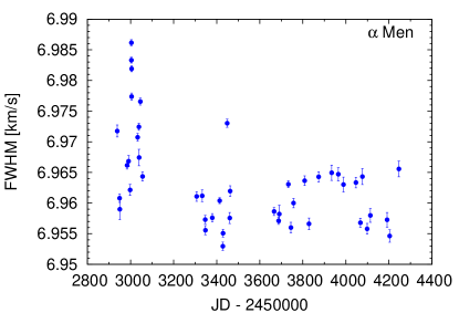
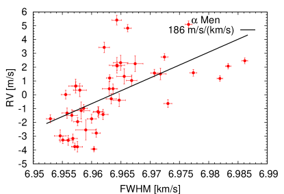
Figure 40: Activity indictors and correlations with HARPS RVs for $\alpha$ Men (2 h binned data, secular acceleration substracted, see Sect. 4.1).

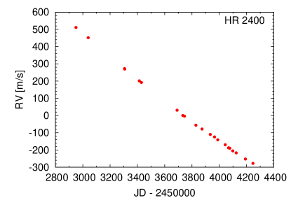
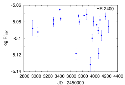
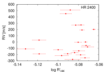
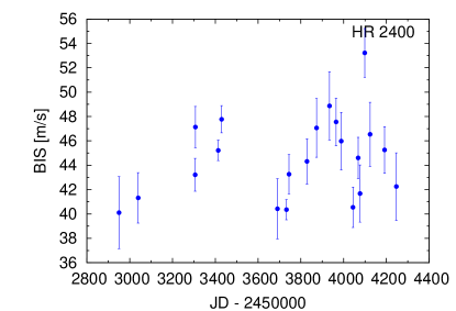
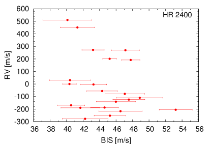
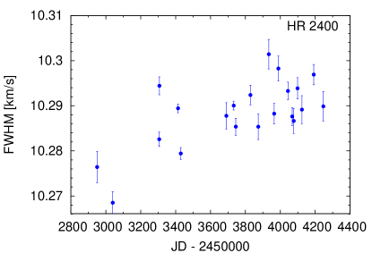
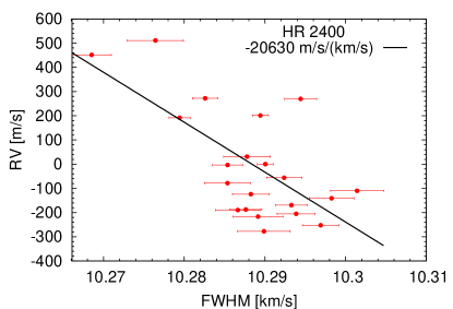
Figure 41: Activity indictors and correlations with HARPS RVs for HR 2400 (2 h binned data, secular acceleration substracted, see Sect. 4.1).

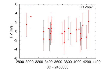
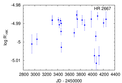
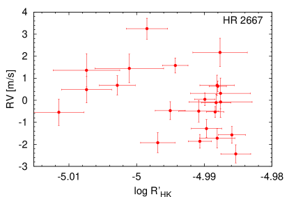
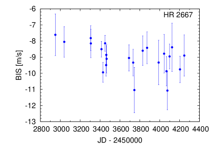
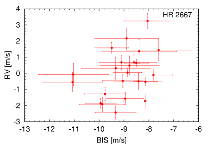
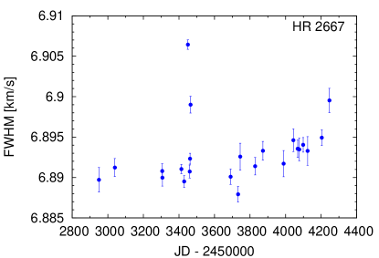
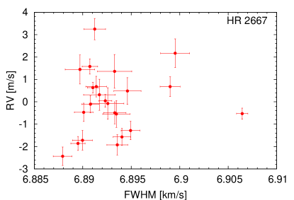
Figure 42: Activity indictors and correlations with HARPS RVs for HR 2667 (2 h binned data, secular acceleration substracted, see Sect. 4.1).

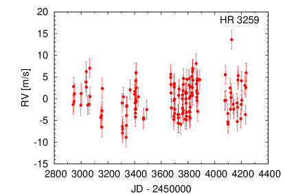
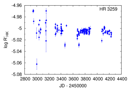
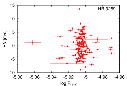
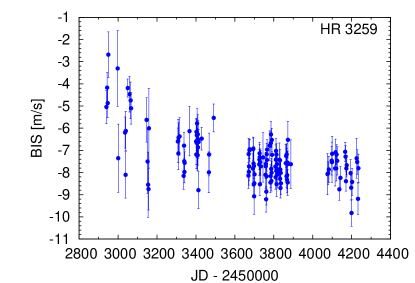
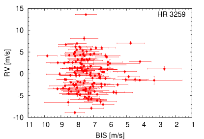
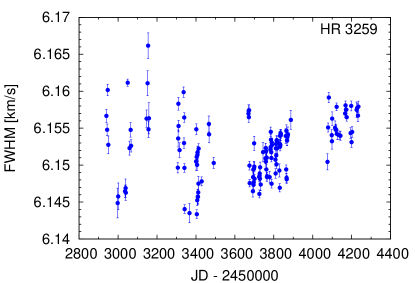
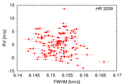
Figure 43: Activity indictors and correlations with HARPS RVs for HR 3259 (2 h binned data, secular acceleration substracted, see Sect. 4.1).

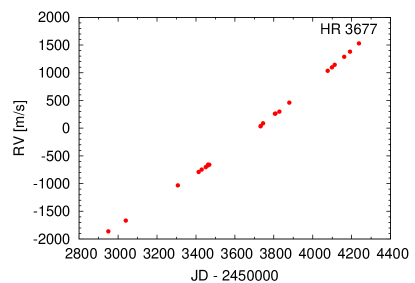
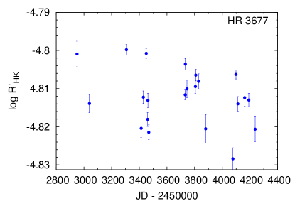
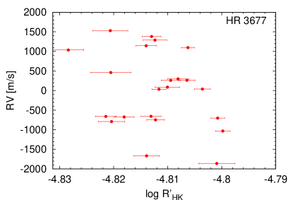
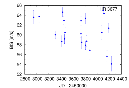
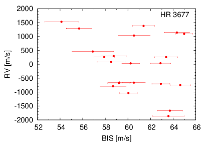
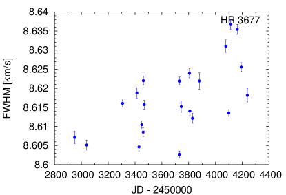
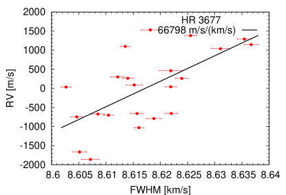
Figure 44: Activity indictors and correlations with HARPS RVs for HR 3677 (2 h binned data, secular acceleration substracted, see Sect. 4.1).

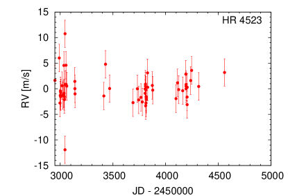
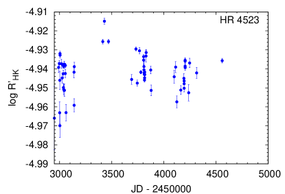
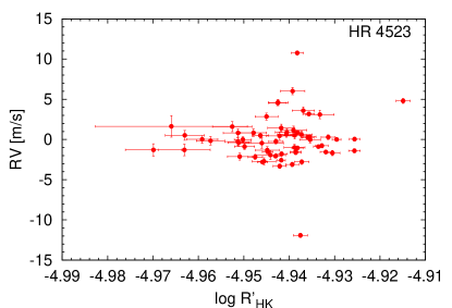
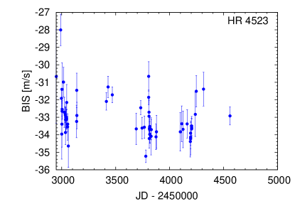
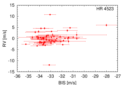
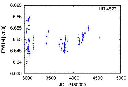
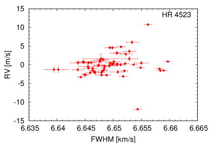
Figure 45: Activity indictors and correlations with HARPS RVs for HR 4523 (2 h binned data, secular acceleration substracted, see Sect. 4.1).

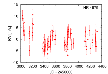
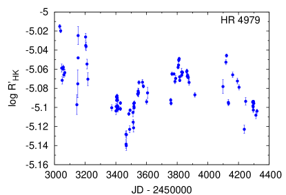
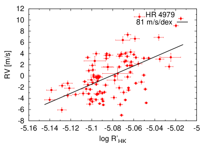
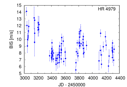
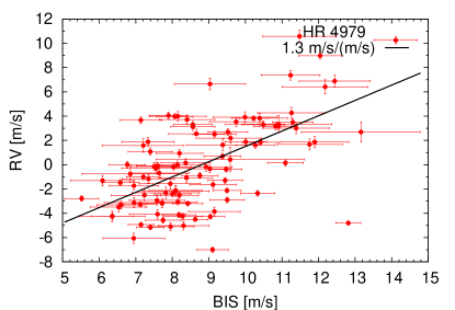
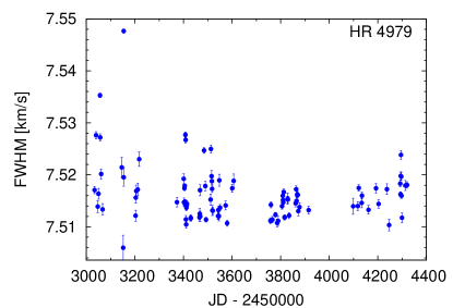
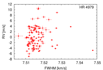
Figure 46: Activity indictors and correlations with HARPS RVs for HR 4979 (2 h binned data, secular acceleration substracted, see Sect. 4.1).

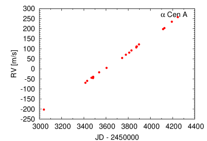
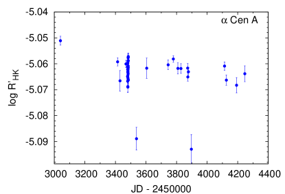
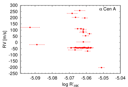
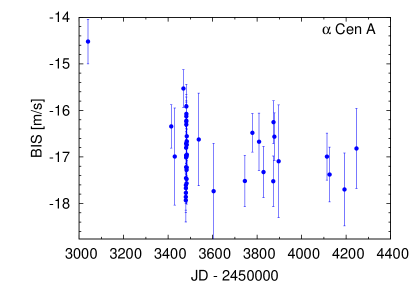
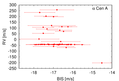
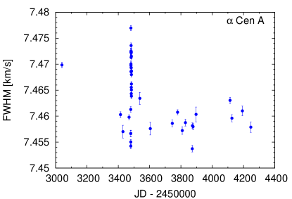
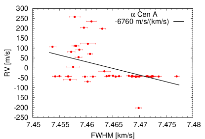
Figure 47: Activity indictors and correlations with HARPS RVs for $\alpha$ Cen A (2 h binned data, secular acceleration substracted, see Sect. 4.1).

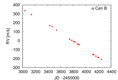
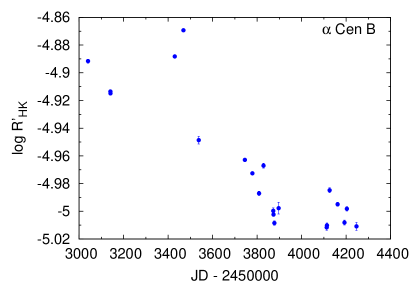
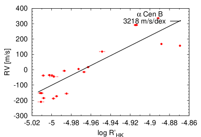
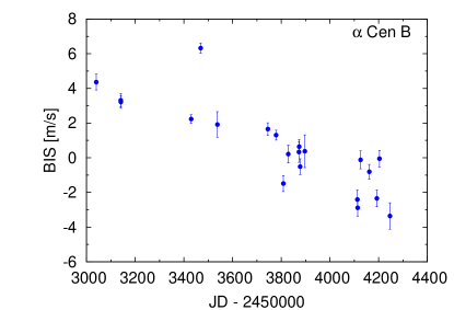
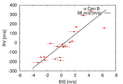
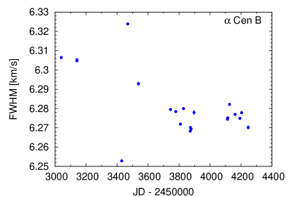
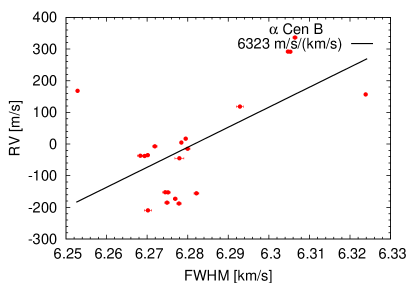
Figure 48: Activity indictors and correlations with HARPS RVs for $\alpha$ Cen B (2 h binned data, secular acceleration substracted, see Sect. 4.1).

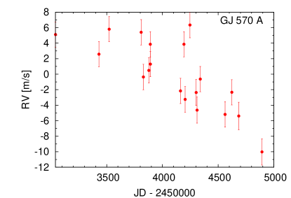
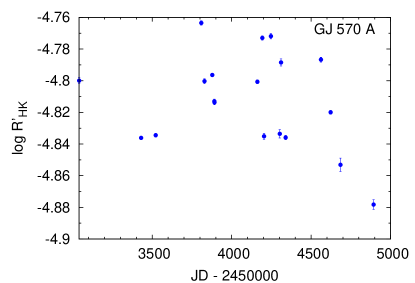
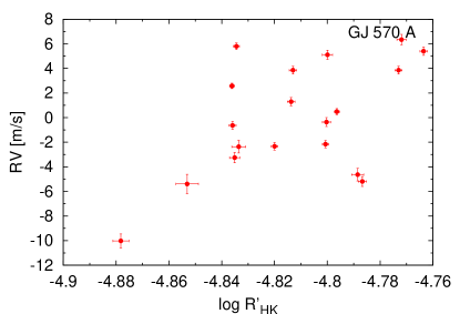
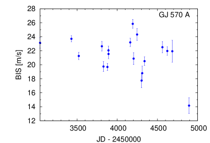
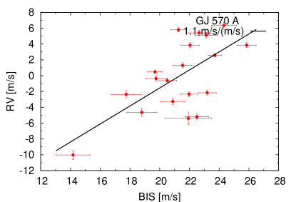
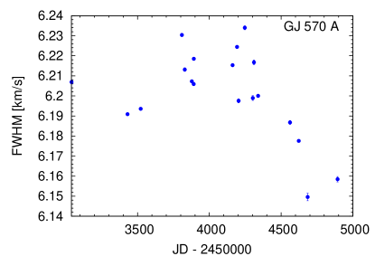
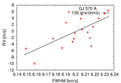
Figure 49: Activity indictors and correlations with HARPS RVs for GJ 570A (2 h binned data, secular acceleration substracted, see Sect. 4.1).

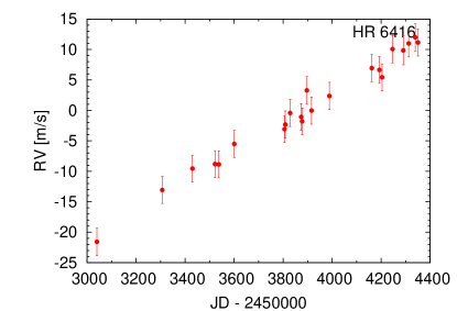
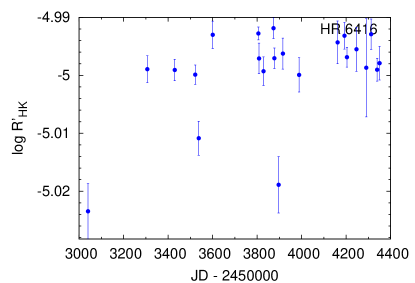
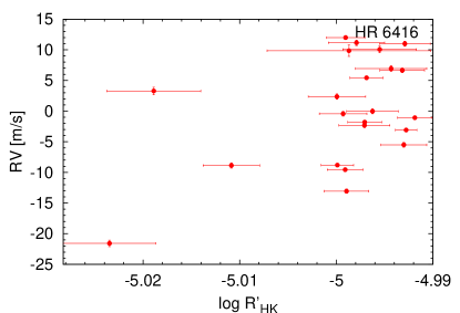
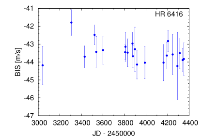
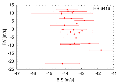
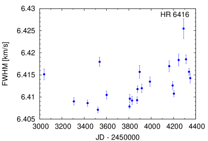
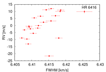
Figure 50: Activity indictors and correlations with HARPS RVs for HR 6416 (2 h binned data, secular acceleration substracted, see Sect. 4.1).

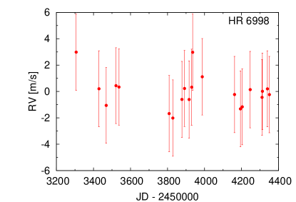
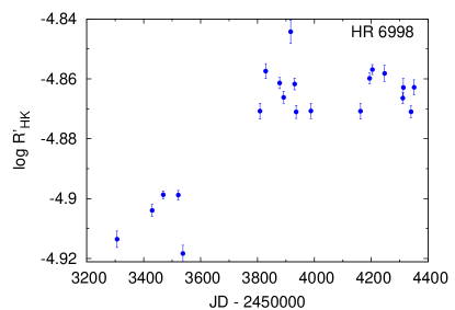
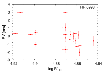
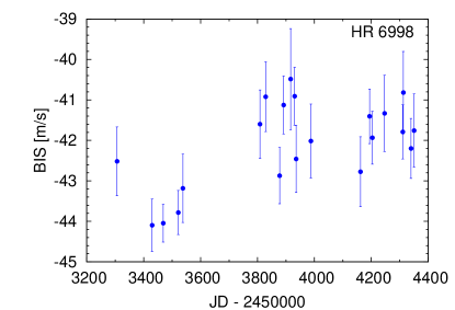
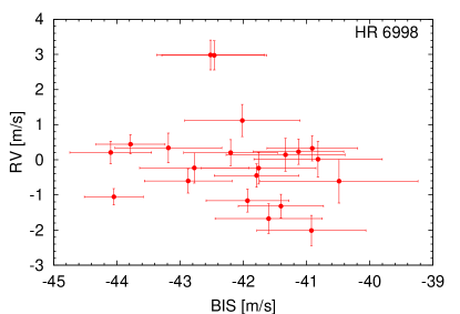
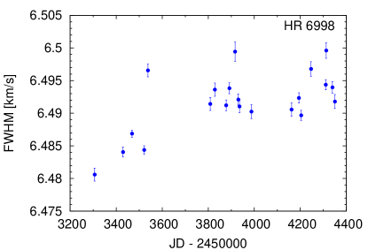
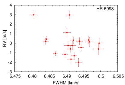
Figure 51: Activity indictors and correlations with HARPS RVs for HR 6998 (2 h binned data, secular acceleration substracted, see Sect. 4.1).

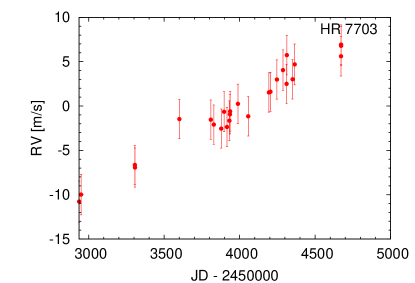
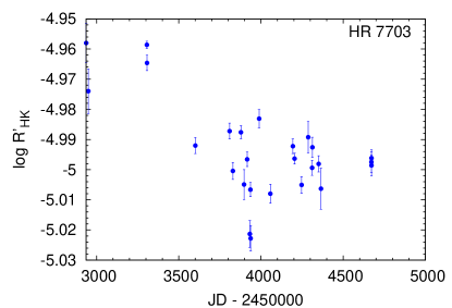
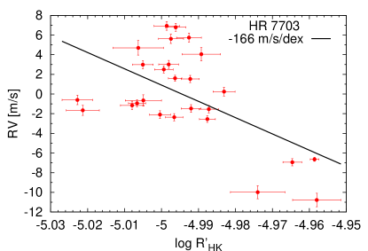
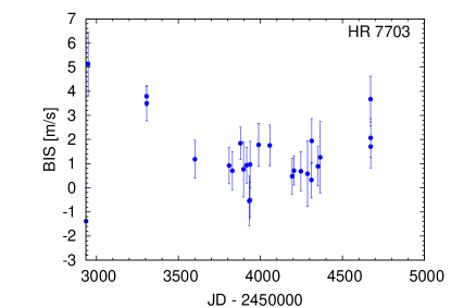
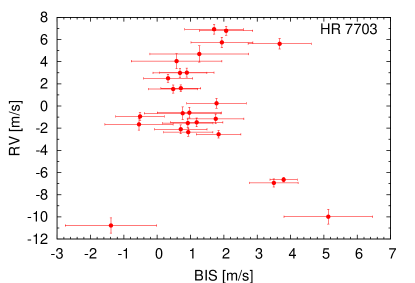
Figure 52: Activity indictors and correlations with HARPS RVs for HR 7703 (2 h binned data, secular acceleration substracted, see Sect. 4.1).

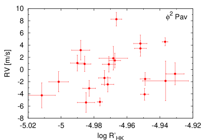
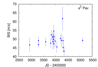
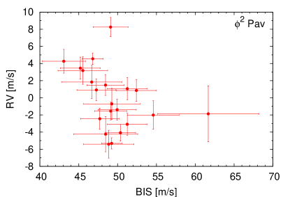
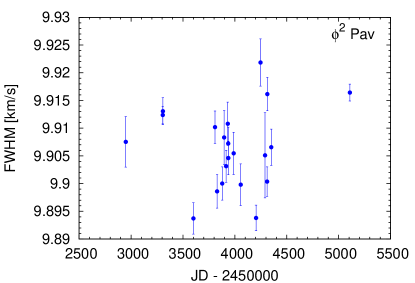
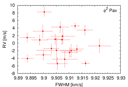
Figure 53: Activity indictors and correlations with HARPS RVs for $\phi^{2}$ Pav (2 h binned data, secular acceleration substracted, see Sect. 4.1).

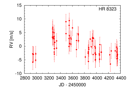
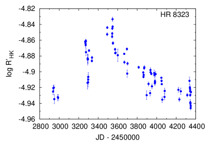
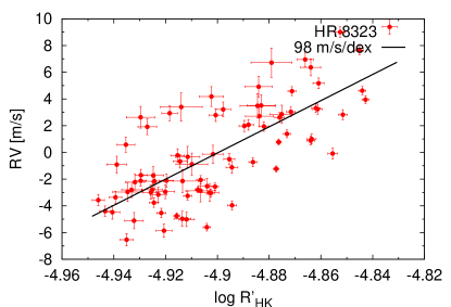
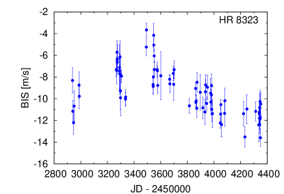
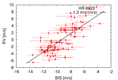
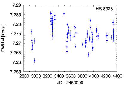
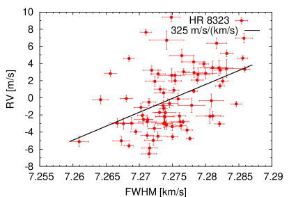
Figure 54: Activity indictors and correlations with HARPS RVs for HR 8323 (2 h binned data, secular acceleration substracted, see Sect. 4.1).

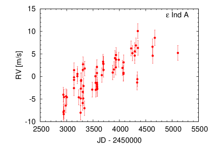
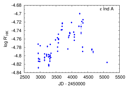
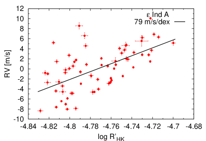
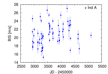
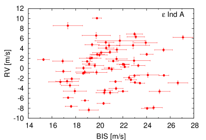
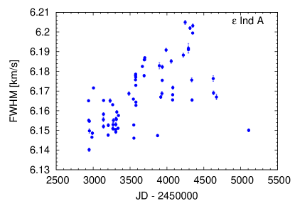
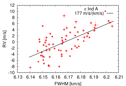
Figure 55: Activity indictors and correlations with HARPS RVs for $\epsilon$ Ind A (2 h binned data, secular acceleration substracted, see Sect. 4.1).

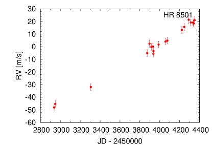
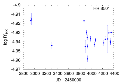
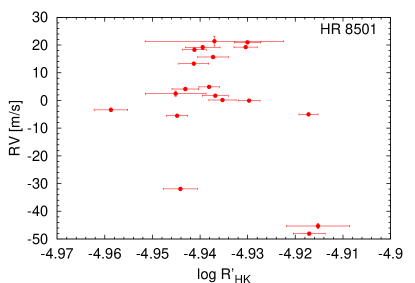
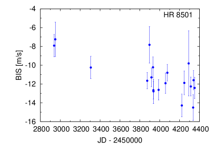
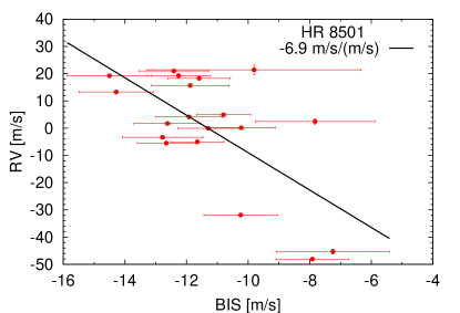
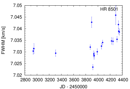
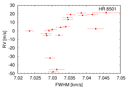
Figure 56: Activity indictors and correlations with HARPS RVs for HR 8501 (2 h binned data, secular acceleration substracted, see Sect. 4.1).

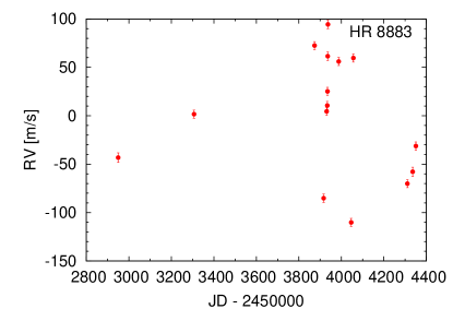
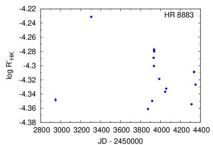
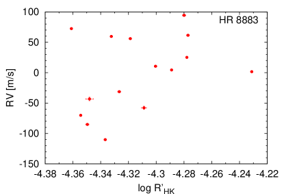
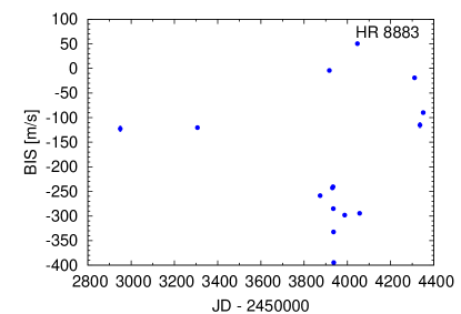
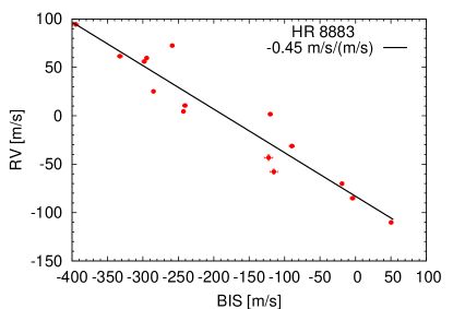
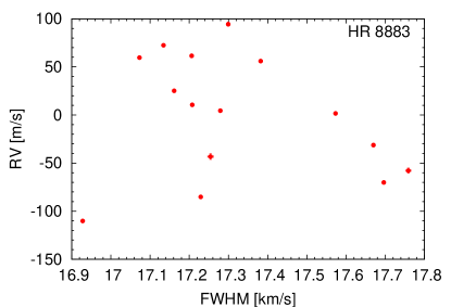
Figure 57: Activity indictors and correlations with HARPS RVs for HR 8883 (2 h binned data, secular acceleration substracted, see Sect. 4.1).