Resonances in open quantum maps
Abstract
We review recent studies about the resonance spectrum of quantum scattering systems, in the semiclassical limit and assuming chaotic classical dynamics. Stationary quantum properties are related to fractal structures in the classical phase space. We focus attention on a particular class of problems that are chaotic maps in the torus with holes. Among the topics considered are the fractal Weyl law, the formation of a spectral gap and the morphology of eigenstates. We also discuss the situation when the holes are only partially transparent and the use of random matrices for a statistical description.
type:
Review Article1 Introduction
A closed quantum system has a discrete spectrum of energy levels, to which are associated bound states. Open systems, on the other hand, have a resonance spectrum, consisting of a discrete set of complex poles of the Green’s function or of the scattering matrix (besides having a real continuous spectrum of scattering states). If we imagine a closed system being slowly opened, its bound states will acquire small (negative) imaginary parts and become resonances. In this sense, the resonance spectrum can also be seen as eigenvalues of a non-hermitian Hamiltonian. If is a complex energy value, the usual time evolution factor is not unimodular but decreases exponentially. The quantity is thus called the decay rate of the state, or equivalently is called its lifetime. Insofar as any real system is always in contact with its environment, most energy levels are actually resonances with a finite decay rate.
We are interested in systems for which the classical dynamics is chaotic. Scattering of waves in chaotic systems has been experimentally realized in a great variety of physical systems. Out of the vast literature available, we select only a few examples: electron transport in semiconductor quantum dots [2, 3, 4, 5] and graphene quantum dots [6, 7, 8]; microwaves in normal metallic [9, 10, 11] or superconducting cavities [12]; nuclear reactions [13, 14]; acoustic waves [15]; microlasers [16, 17, 18].
In the semiclassical limit the wavelength is much smaller than any classical length scale and the nature of the classical (or ray) dynamics becomes important. Three main questions then stand out in connection with the resonance spectrum of a chaotic scattering system. First, how does the number of resonances with given decay rate grow with ? Second, is there a lower bound for the decay rates? Third, what do the resonance wavefunctions look like (inside the scattering region)? As we will see, all these questions are related to fractal properties of the classical dynamics. They are all still open to some extent, although much progress has indeed been made.
The systems we have in mind have ‘classical’ openings. By this we mean the following. For a fixed value of the energy, a finite ‘energy shell’ can be constructed by imagining a big enough box enclosing the scattering region in configuration space and all possible momenta with fixed magnitude. In this energy shell, the points leading to immediate escape occupy a finite volume. In this situation the resonances are always strongly overlapping (sometimes called the Ericson regime).
A very popular class of models with which one can theoretically study chaotic scattering are so called torus maps, some of which are well known like the baker map or cat maps. These toy models have the maximal simplicity still allowing for chaotic dynamics. Also, they can be quantized in order to study wave properties. In the last few years, the resonance spectrum of open quantum maps has been widely studied and have shed considerable light on the more general problem. Our purpose is to review these developments.
Other reviews concerning areas related to the ones discussed here have appeared recently and can offer complementary insights. Open systems and non-hermitian Hamiltonians were reviewed by Rotter in [19] and, from a very different point of view, by de la Madrid and Gadella in [20] (see also [21]); open billiards were reviewed by Dettmann in [22] and also by Altmann, Portela and Tél in [23]; the random matrix theory (RMT) approach to resonances in quantum systems was reviewed by Fyodorov and Savin in [24] and by Mitchell, Richter and Weidenmüller in [25]. Finally, spectral results for chaotic open maps were reviewed by Nonnenmacher in [26], but from a mathematically more rigorous perspective than the one adopted here.
In Section 2 we introduce open chaotic maps. We give a few examples and discuss their long time behaviour. We introduce fractal trapped sets and conditionally invariant measures. In Section 3 we discuss open quantum maps and their general properties. Section 4 is dedicated to the fractal Weyl law that has been conjectured to hold for the resonance spectrum in chaotic scattering. Section 5 discusses the possible existence of a spectral gap. The phase space morphology of resonance wavefunctions is considered in Section 6. In Section 7 we focus on systems where escape is not ballistic, like e.g. microlasers. The RMT approach to quantum scattering is discussed in Section 8. Finally, we close in Section 9 with some open problems.
Let us mention that we do not consider the closely related, and somewhat complementary, transport formulation of scattering [27], which deals with matrices, transmission eigenvalues, counting statistics, etc. The semiclassical and the RMT approaches to quantum chaotic transport were reviewed, for instance, in [28] and [29], respectively.
2 Classical maps
When studying the integrability of the dynamics of the solar system, Poincaré introduced the idea of ‘cutting through’ phase space with a hyperplane, and recording the intersections of the system with this plane. This construction, now known as a Poincaré section, produces a discrete-time dynamics in which the trajectory becomes a sequence of points. The time interval between intersections is lost, but this is usually considered a small price to pay for the dimensional reduction achieved.
We consider maps in themselves, without any reference to a continuous-time system from which they could be derived. We shall treat only maps that are defined on a two-dimensional torus, which can be represented simply as a square with opposite sides identified. Let us denote by orthogonal coordinates in this space which are the sides of the square. We have in mind conservative chaotic dynamics (hyperbolic and mixing).
Let denote the map. If , we say that the point evolves into the point . An infinite sequence of points is called an orbit. If an orbit consists in the infinite repetition of a finite number of distinct points, it is called periodic. The number of distinct points is then its period. Its is known that chaotic systems have infinitely many periodic orbits, and that they form a dense set in phase space, i.e. there is a periodic orbit arbitrarily close to any point.
Many books discuss chaotic maps. We just mention for example [30, 31], where all basic definitions, examples and further discussion can be found. In the following, we briefly present a few paradigmatic systems and introduce only the notions that will be needed when we consider the resonances of open quantum maps.
Perhaps the simplest example is the baker map, given by
| (1) |
Its well-known dynamics consists in a stretching by a factor of along the axis, together with a contraction by the same amount in the axis, plus a ‘cut and paste’ operation involving the line . Clearly, area is preserved. Also, the map is hyperbolic, with stable and unstable directions at every point being parallel to the coordinate axes. The Lyapounov exponent is . Notice that the baker map may be written as
| (2) |
where denotes the integer part of .
Many generalizations of the baker map exist. One of them makes use of basic regions, stretching and compressing by a factor of :
| (3) |
This is sometimes called the -nary baker map. The usual baker map corresponds to . This map has a Markov partition with cells, and each cell is stretched and compressed by a factor at each iteration. Therefore, the Lyapounov exponent in this case is .
The so-called cat maps provide another paradigmatic family of chaotic linear maps. The following is an example:
| (4) |
In this case the Lyapounov exponent is . The dynamics of cat maps has no discontinuity. The stable and unstable directions are still the same at every point, but they are no longer orthogonal.
Our final example will be the standard map. It is defined as
| (5) |
It is more generic than the previous examples because it is non-linear. Its dynamics is known to be predominantly chaotic if . The stable and unstable directions, as well as the local stretching factor, are no longer constant in phase space. It is known that the Lyapounov exponent (the average stretching factor) is given approximately by .
Instead of propagating points, it is often useful to consider propagation of probability measures. Given a probability measure , its evolution is another probability measure such that, for any subset of phase space, . A measure is called invariant if for every . If we allow singular invariant measures, such as linear combinations of Dirac deltas, then clearly there are infinitely many of them (for example, to any periodic orbit we can associate one).
If a probability measure has a probability density , such that , it is called absolutely continuous. Probability densities can also be evolved in time: if , then the function such that is called the evolution of (remember that the map is conservative, so there is no Jacobian). In other words, each point simply carries along the value of the function associated with it. The linear operator that implements this evolution, , is called the Perron-Frobenius operator associated with the map .
All examples of chaotic maps discussed previously are ergodic systems and hence have only one invariant probability density. This is called the natural density or equilibrium density, denoted (for conservative maps this is simply the constant function). They also have the exponential mixing property, which implies that any smooth initial density function will converge to exponentially fast in time (when defined on an appropriate function space, has a single eigenvalue equal to and all other eigenvalues have strictly smaller modulus). This convergence of course takes place in a weak sense.
We now wish to consider open maps as models of chaotic scattering. Given a map, an open version is obtained by defining a ‘hole’ in phase space, which can in principle be any region of finite area (or union of regions). Once a point falls into the hole, it stops being propagated (i.e. it ‘escapes’). This means that the dynamics is no longer conservative. In fact, for chaotic systems almost all initial conditions eventually escape because of ergodicity. We denote by the open map, i.e. the map that acts by first removing points in the hole and then evolving the remaining ones according to .
The trapped set of the dynamics is the set of initial conditions which do not originate from the hole and never hit the hole. In other words, they remain in the system for infinite time, whether propagated forwards or backwards. This invariant set will be denoted . It is quite common in the quantum chaos literature to refer to as the system’s ‘repeller’. This has been criticized on the grounds that ‘repeller’ should be used for sets that are unstable in all directions. When a stable manifold exists, [23] and [32] suggest calling the chaotic saddle or simply the ‘saddle’. We shall follow this suggestion.
The stable manifold of the saddle, the set of points which converge to it and therefore never escape in the future, is also known as the forward-trapped set and denoted . On the other hand, the unstable manifold contains the initial conditions which never escape in the past and is also called the backward-trapped set . These two sets are fractals and have similar structures. Globally, they are very convoluted. Locally, they are continuous in one direction and fractal in the orthogonal one. Therefore, they both have zero measure in phase space.
The sets and can be described in terms of images and pre-images of the hole. Let be the th image of the hole under the dynamics. The set is the hole itself. These sets can have finite intersections, so we define another family of sets as . The set contains the points that fall into the hole in exactly steps when propagated backwards. Analogously, we can start with and for define as the set of points which fall into the hole in exactly steps when propagated forwards. These sets obey , and
| (6) |
Let us imagine that we start with the torus completely filled with initial conditions, and they are all propagated forwards. First, the points at the hole escape. Then, the points that were initially at escape. Next, the points initially at , and so on. Clearly, since it contains the points that never escape, the forward trapped-set must be the complement of the union of all . On the other hand, the backward-trapped set is the complement of the union of all . Notice that the sets intersect the unstable manifold and in fact provide a useful partition of it (every point of is either in one of the or belongs to ).
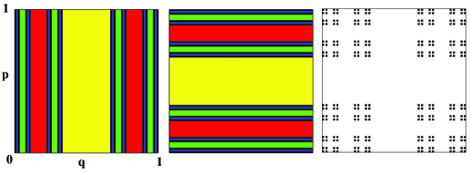
The simplest example of open map with a nontrivial saddle is the ternary baker map with the middle region identified with the hole. This is discussed in detail, for example, in [33]. It is easy to see that all sets consist of vertical strips. The horizontal section of , for example, is . The set is always the union of strips of width . As a matter of fact, the forward trapped set is the product of the interval in the vertical direction and a Cantor set in the horizontal direction. Analogously, the backward trapped set is a Cantor set in the vertical direction. Finally, the saddle is the product of two Cantor sets. This example can be seen in Figure 1, while the analogous construction for the kicked rotator is shown in Figure 2.
Open systems can have invariant measures, but they must be supported on the saddle and thus are very singular. Let denote the -step propagation of measure . A measure satisfying is called an eigenmeasure of the system. Invariant measures correspond to .
Incidentally, open systems provide a glimpse at how truly vast is the set of invariant measures for closed ones. A closed system can be opened by choosing any region of phase space as the hole. In turn, this may generate a chaotic saddle, which can carry many invariant (singular) measures. These are also invariant measures of the closed system, and we thus have many such measures for many possible choices of hole in phase space.
Eigenmeasures with are called conditionally invariant measures (in the sense that they are invariant provided we renormalize them at every step). Conditionally invariant measures for maps were reviewed in [34]. They are necessarily supported on . Since this set has a fractal ‘cross section’, they cannot be absolutely continuous. If we take smooth initial measures and propagate them forwards, they all still converge (when renormalized) to the same measure , called the natural measure or equilibrium measure. It is an eigenmeasure satisfying
| (7) |
The quantity appearing in (7) is called the system’s decay rate. Decay rates for chaotic systems with holes have been reviewed in [23]. In the limit of vanishingly small holes, is given simply by the size of the hole. For finite holes, however, it is in general a complicated function of its size, shape and position (see the many references in [23]). For example, the decay rate can be reduced if the hole contains a short-periodic orbit, because this implies that it overlaps considerably with its images, reducing the amount of points that escape after one step (this was observed for example in [35, 36, 37, 38]).
A formula for is available in terms of the equilibrium measure [39]:
| (8) |
where is the -measure of the hole . This can be understood as follows: for long times any initial probability measure converges to , and gives the proportion of points which escape at one time step, which must be equal to . It is also possible to compute using a sum over periodic orbits contained in the hole [30, 31].
One important characteristic of a fractal set is its dimension. Because is a simple line in one direction, its total dimension is given by
| (9) |
where is called the partial fractal dimension. If the dynamics has time-reversal symmetry, then has exactly the same dimension as . Their intersection, , is locally equal to the product of their fractal parts and thus has
| (10) |
as its dimension (for systems without time-reversal symmetry, the dimension of is the sum of the partial dimensions of and ).
We only consider fractal sets (, and ) characterized by a single fractal dimension (i.e. their Minkowski and Hausdorff dimensions coincide). For fractal measures, on the other hand, different notions of dimensions coexist. The most used ones are the Minkowski (or box-counting) dimension , the information dimension and the correlation dimension . These are in principle distinct but in most practical situations they happen to be quite close to each other. It is known that they can be generalized to a continuous function which is non-increasing (the so-called Rényi dimensions), so .
We are only interested in the natural measure . Since it is supported on , its Minkowski dimension is given by . Since it is continuous in the direction of , we can write, for every , the corresponding dimension in terms of a partial component:
| (11) |
We will use without a subscript for the fractal sets and with a subscript when we refer to dimensions of the natural measure. It is quite common, however, to talk about when one means , because of the uniqueness of the natural measure. It is well known that there exists an important equation (the Kantz-Grassberger relation [40]) involving the decay rate, the Lyapounov exponent and the partial information dimension of . This is
| (12) |
Coming back to the open tribaker map, if we fill phase space uniformly with initial conditions, then exactly one third of points will hit the hole at each step, leading to . The partial dimension of is the fractal dimension of the Cantor set, well known to be . The natural measure is constant on and, therefore, all its fractal dimensions are the same, . This is not a general feature; it comes from the fact that the stretching rate is constant for this system. Notice that the Lyapounov exponent is , so that the relation (12) is indeed verified.
In Section 7 we shall discuss maps for which escape is not ballistic, i.e. when a point falls in the hole, it has a certain probability of escaping but can also continue being propagated. A probability density is then only partially attenuated when coming in contact with the hole, instead of being drastically cut. This is supposed to model, for instance, refractive escape of light rays from a dielectric sample.
3 Quantum maps
Maps have long been used as toy models in classical mechanics, because they allow for chaotic conservative dynamics even in a two-dimensional phase space. But they have also enjoyed popularity in the context of quantum mechanics, the reason being that their numerical implementation is quite simple. When a map is defined on a compact phase space, for example, its quantum propagator is automatically finite dimensional.
Unlike for Hamiltonian systems, there is no standard procedure to quantize a map. The general idea is that, given a conservative classical map , one should associate with it a unitary operator (the propagator) acting on some Hilbert space. Naturally, some kind of classical limit must be defined, in such a way that the dynamics of is recovered.
Since we are considering only the torus as our phase space, we must enforce periodicity both in and in . This implies that both directions become discretized, i.e. there will be a finite number of ‘position’ eigenstates and ‘momentum’ eigenstates . Quantization of classical periodicity can be achieved with a pair of arbitrary phases, so that
| (13) |
For given values of and , the corresponding coordinates on the torus are
| (14) |
The case corresponds to periodic boundary conditions, while correspond to antiperiodic boundary conditions. Position and momentum must be Fourier related,
| (15) |
Here both and range from to . The dimension takes the role of inverse Planck’s constant:
| (16) |
Quantization of the dynamics consists in the construction of a quantum propagator , which is a -dimensional unitary matrix responsible for taking one wavefunction to another:
| (17) |
This operator can always be diagonalized, and its spectrum lies in the unit circle in the complex plane, namely all eigenvalues are of the form with .
The matrix must somehow reproduce the classical dynamics in the limit . To visualize this limit one usually resorts to tools such as coherent states and Husimi functions. In usual quantum mechanics, coherent states are ground states of harmonic oscillators, i.e. Gaussian wavepackets with minimum uncertainty. When realized in the torus, they must incorporate periodicity (a recent review about coherent states can be found in [41]). Therefore, they are defined in position representation as
| (18) |
where is a normalization constant.
The Husimi function of a quantum state is a real, non-negative function defined over all phase space. It can thus be normalized and interpreted as a probability density (however, it does not have the correct marginals, e.g. ). The Husimi function of a coherent state, , is a periodized Gaussian in both directions, centered at the point , with widths .
For large , the action of the quantum propagator on coherent states must satisfy the semiclassical condition , i.e. it must take the point to its image under the classical map. Actually, this evolution will always introduce a stretching of the wavepacket along the unstable direction, coming from the Lyapounov exponent. It is more correct to say that the action of the quantum propagator must correspond, in the semiclassical limit, to the action of the Perron-Frobenius operator: it takes an initial probability distribution centered at (the Husimi function of the state ) to another probability distribution which is centered at (but is not the Husimi function of the state ).
This semiclassical approximation cannot hold for long times due to interference effects. The similarity between the action of on the quantum side and on the classical side must degrade with time . For chaotic systems, it degrades exponentially fast. Heuristically, it will break down at the time scale given by the time it takes a minimum wavepacket (of width ) to stretch to the size of the system. This is called the Ehrenfest time and, since the stretching is regulated by the Lyapounov exponent according to , it is given by .
Notice that other definitions of Ehrenfest time are possible. For example, the time it takes to stretch a state which is squeezed along the stable manifold into a state which is squeezed along the unstable one is . This is equivalent to stretching the smallest length, , to the size of the system and has also been called the Ehrenfest time in the literature (indeed this is the time when some interference effects start to become important, see for example [42]). Yet another notion of Ehrenfest time, related to escape through holes, will be presented below. The quantum-classical correspondence for open chaotic systems, with special emphasis on different Ehrenfest times, was reviewed in [43].
Let us now mention, without any technical details, some of the quantizations that have been devised for the classical maps discussed in the previous section.
The first quantization of the baker map, introduced in [44], postulated the following propagator:
| (19) |
It is compatible with periodic boundary conditions and can only be defined on even-dimensional spaces, reflecting the nature of the underlying map. It can be verified that this operator has the baker map as its classical limit, but an inversion symmetry of that map does not hold exactly. Later [42], another quantization with antiperiodic boundary conditions was suggested, that had exact symmetries. In this quantization is replaced by .
The quantization of cat maps was considered in [45, 46, 47]. Here the fact that the classical action is quadratic was used to define a semiclassical quantization. For the particular cat map (4) we mentioned previously, this results in a matrix whose elements are quite simple:
| (20) |
with between and .
Finally, the standard map can also be quantized [48, 49]. It can be realized as a kicked rotator, which leads to a quantization in terms of the product of free propagation and kicking. More convenient is the following closed formula in position representation:
| (21) |
This actually corresponds to a version of the system which displays time-reversal symmetry.
A few experimental realizations have been suggested for the quantum maps discussed above. In [50] an optical set-up of the baker map was proposed, while a possible realization using nuclear magnetic resonance was discussed in [51]. Already in [45] the possibility of realizing the quantum cat map using Fresnel diffraction by a periodic grating was suggested. Finally, the quantum kicked rotator has already been realized in the laboratory by placing cold atoms in a pulsed standing wave [52, 53].
It is natural to expect that in the semiclassical limit the Husimi functions of eigenstates of should converge, in some weak sense, to invariant probability distributions. As we have seen, these are either related to or singular. It is known that, as , almost all eigenstates will become equidistributed, i.e. their Husimi functions will converge to . In other words, as one diagonalizes in larger and larger dimensions, the fraction of equidistributed states should grow to . This property is called quantum ergoditicy. A stronger property is that of quantum unique ergodicity. This property holds when we can say that all quantum states become equidistributed without exception, which is a stronger statement than saying that their fraction becomes . Quantum ergodicity and quantum unique ergodicity have been extensively investigated for cat maps and baker maps (see, for example, [57, 58, 59, 60]). A recent review appears in [61].
Numerically, it is easy to find for finite some eigenstates with Husimi functions concentrated on periodic orbits. This phenomenon has been termed ‘scarring’. For continuous-time systems, there is a large literature on this subject starting with [54]; for maps see [55, 56] and also [61].
In order to open a quantum map, what we have to do is identify a sector of the Hilbert space with the hole. This is done by ‘projecting out’ of it, i.e. the open propagator is
| (22) |
where is the closed propagator and is the projector on the complement of the hole. It is most common to use a hole that is a strip of width parallel to the momentum axis. In that case will be diagonal in position representation. The value of sets a new length scale in the problem [43]. We can define the escape Ehrenfest time as the time it takes to stretch the fundamental size up to . This satisfies . If we let be the number of quantum states that fit in the hole, i.e. the dimension of the kernel of the projector , then clearly .
The eigenvalues of will be located inside the unit disk in the complex plane. They can be written as
| (23) |
so that can be interpreted as a decay rate (it corresponds to what was in the more general Hamiltonian setting). The set of all eigenvalues comprises the resonance spectrum of this ‘scattering’ problem. Resonances in the vicinity of the origin as seen as short-lived, while any finite value of can be understood as being long-lived.
4 Fractal Weyl law
The Weyl law is a very basic result in the asymptotics of energy levels for closed systems. In a nutshell, it says that each stationary quantum state occupies a volume in phase space, where is the number of degrees of freedom [62]. This means that, to leading order in , the number of states with energy less than is proportional to . Alternatively, let be the set of phase space points with energy . It is obvious that this set has dimension . The density of states around is then proportional to the size of and scales with as .
For open systems, a similar idea can be applied to the resonance spectrum. One can choose a small but fixed region of the complex plane, around a point with real part and imaginary part (such that the decay rate is fixed), and ask how the number of resonances inside it grows as . For continuous-time chaotic flows, it is conjectured that this number should behave like , where now is the fractal dimension of the classical chaotic saddle at energy . This is known as the fractal Weyl law (FLW). In the context of continuous time, it has been checked for scattering from three gaussian ‘bumps’ [63, 64], three rigid disks [65], four rigid spheres in 3D [66] and a modified Hénon-Heiles potential [67]. The only rigorous result available to date is that the exact number of resonances is bounded from above by the FWL [68, 69].
A vague heuristic justification of the FWL can be presented as follows (a more detailed account is given in [63]). States with energy have lifetime . From basic principles, these states should be related to structures in classical phase space which remain inside the system for that long. By analogy with the usual Weyl law, their number is estimated as being proportional to the volume of a ‘coarse-grained’ version of the saddle, of thickness proportional to . As , this volume is related to the fractal dimension.
The FWL takes on a particularly simple form for quantum maps, because of dimensional reduction, no energy-dependence of the dynamics and the fact that the total number of resonances is equal to . In that case the conjecture is that the number of resonances with modulus larger than some should grow like , where is some unknown function of and is the fractal dimension of the saddle discussed in Section 2. Notice that
| (24) |
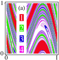
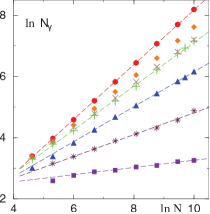
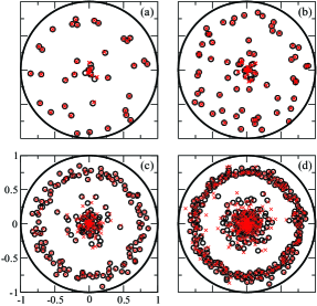
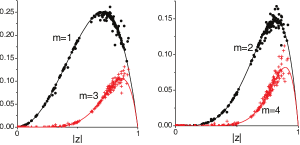
where is the dimension of the backward trapped set and is the associated partial dimension. In [33, 70] the FWL was verified numerically for the open triadic baker map and rigorously proven for a non-canonical quantization of this map. It has also been verified for the kicked rotator [71, 72] and for the cat map [73]. Again, only upper bounds can be rigorously proven [74]. In Figures 3 and 4 we show numerical verification of the FWL for three types of open quantum maps.
What is the function ? The first point that needs to be settled is whether this function is universal or system-dependent. For the kicked rotator [71] it is quite close to the universal prediction from random matrix theory (see Section 8), but this is not true for the baker map [33]. In fact, in this latter case there seems to be a gap in the middle of the spectrum, for which no explanation has been offered so far. If the function is system-dependent, it remains to be determined what kind of classical information goes into it.
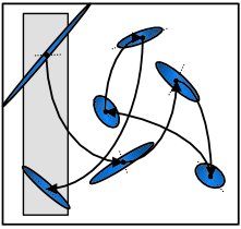
One theoretical approach to the FWL, put forth in [71], is via the construction of short-lived states. We sketch its argument. Let be the dimension of the kernel of (the number of quantum states that fit in the hole). Let and be the Lyapounov exponent and the escape rate of the system and let be the (escape) Ehrenfest time. Remember that is the set of points that escape in exactly steps. A minimal wavepacket supported in will therefore reach the hole in steps. If is smaller than , this wavepacket will not have spread too much and will still fit in the hole. It will then be almost completely annihilated and we will have , i.e. it will be a generalized eigenvector of with zero eigenvalue. This process is illustrated in Figure 5.
What we mean by saying that is a generalized eigenvector is that and its images under form a Jordan chain. In other words, the fractal Weyl law is related to the difference between the algebraic and the geometric multiplicity of the null eigenvalue. These ideas were further discussed in [75], where it was suggested that, instead of being diagonalized, the open map should be subject to a Schur decomposition, , where is unitary and is upper triangular. This has the advantage that, unlike the eigenvectors, the columns of are orthogonal.
In essence, this identifies the states comprising the short-lived sector of the resonance spectrum. To estimate their fraction, we need only estimate the total area of all with up to . Since the fraction of points remaining after steps is , that area behaves like . Therefore, the short-lived sector amounts to a fraction of the spectrum that scales as . Since is proportional to , this implies that the total number of states in the long-lived sector, which is counted by the fractal Weyl law, should scale as where is the partial information dimension of the natural measure .
The above arguments provide some understanding of the physical origins of the FWL, but the exponent they predict is instead of . Rigorous upper bounds involve . Still, the information dimension was also used in [72], where the kicked rotator is studied in a range of decay rates, and again in [73] for the cat map with several different holes. In both these works very good numerical agreement was obtained. On the other hand, it was shown in [76] that the true exponent really is closer to by explicit construction of a system where and are very different. In general, however, these two dimensions are quite close; large deviations can only be expected for systems where the local stretching factor is very far from being constant (which is the case in [76]).
Another approach to the FWL was developed in [77] and [78]. This is based on semiclassical approximations for the long-lived states, and the basic idea is that these should be related to periodic points, which belong to the saddle. An approximate basis for the long-lived sector is constructed by building wavepackets concentrated on periodic orbits of period , with up to . These wavepackets are then propagated with the open quantum map, thereby acquiring some information about short-time dynamics and providing an improved basis, the so-called scar functions. Since the number of points with period less or equal to grows like (the quantity is the Kolmogorov-Sinai entropy), the dimension of the basis is proportional to . A matrix of this dimension is then introduced as an approximation of the quantum propagator in the long-lived sector. Its spectrum is in good agreement with exact results, validating the approximation. This is shown for the baker map in Figure 6. Notice the presence of a gap in the bulk of the spectrum.
This semiclassical approximation was critically discussed in [79], where it is argued that it reproduces the spectrum, but in order to correctly describe quantum resonance wave functions semiclassically it is necessary to take into account more information than only the chaotic saddle. The authors of [79] speculate that diffraction effects and/or classical information outside the saddle should be important and must be incorporated. This is yet to be systematically investigated. Another point raised in [79] is that perhaps in practice the fractal Weyl law only holds once becomes much smaller than the size of the hole, otherwise it may be affected by diffraction.
In [74] a rigorous theory was developed to the construction, based on an open quantum map of dimension , of an auxiliary operator whose rank is and whose spectrum reproduces the exact resonances. That operator is conceptually similar to the one based on short periodic orbits that was discussed above.
Notice that the two approaches we just delineated are different and somehow complementary to each other. While [71] arrives at the FWL by estimating the size of the short-lived sector, associated with regions of fast escape, [77, 78] attempt to estimate the size of the long-lived sector, expected to be related to periodic orbits. In both cases some notion of Ehrenfest time plays an important role.
The Weyl law for systems whose dynamics is a mixture of chaotic and regular regions was discussed in [75]. It was found that stability islands led to resonances with very small decay rate, approximately following a usual Weyl law, while states with intermediate decay rates obeyed a Weyl law with a fractional exponent; however, this exponent was not related to the dimension of any fractal set. The subject was also investigated in [80] for a system with sharply divided phase space. States associated with sticky motion at the border of the stability island satisfied Weyl laws with fractional exponents, related to the power law behaviour of the classical survival probability.
5 Resonance gap
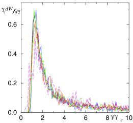
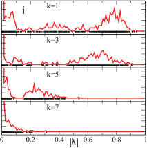
The fractal Weyl law is a prediction about how the number of long–lived resonances scales with or, for quantum maps, with the dimension . A different type of question is how these resonances are distributed in the complex plane. For maps, we denote them by , so that . In particular, it is natural to focus interest on the longest-lived ones because they usually leave clear signatures on scattering signals. Numerical experiments reveal that the distribution of decay rates tends to have a maximum around the classical decay rate , with a long tail for and a rather short one for . This has been observed for example in [72, 81, 82, 83], and we show an example in Figure 7.
In a sense, states with have anomalously slow decay. They were termed ‘supersharp’ resonances in [84]. A natural question is whether there is a limit to how sharp a resonance can be. Can the quantum decay rate be arbitrarily small? Evidence is on the contrary. It is generally expected that supersharp resonances should become less frequent in the semiclassical limit, i.e. that a true gap develops in the spectrum as .
Already in [85] (see also [86]) it was found that a lower bound could be proved for the decay rates of chaotic resonances in the limit . Its formulation involves something called the topological pressure . This is related to the leading eigenvalue of a generalization of the Perron-Frobenius operator introduced by Ruelle. We do not discuss this so-called thermodynamic formalism here, and instead refer the reader to [87, 30]. The topological pressure has some important properties, namely its value at gives the decay rate, , its derivative at this point gives the Lyapounov exponent, , and it has a zero at the partial dimension of the unstable manifold of the saddle, . For the open triadic baker map it is given by ; in general it is a convex decreasing function.
The available rigorous lower bound is that all must be larger than as . This result has been revisited recently with more rigor in [88]. Interestingly, this bound is only effective if , because is a decreasing function with a zero at , so if . This would just predict that all are larger than a negative value, something that is always true. In other words, only for saddles that have low enough dimension, or are ‘filamentary’ enough, can a true lower bound really be established.
It is known that and hence is always smaller than the classical decay rate . Therefore, this lower bound still allows for quantum decay that is slower than classical. At present, it is not clear whether in the limit one can still find resonances with decay rate arbitrarily close to or if they tend to be larger than . In other words, if a larger gap can appear. An approach based on random matrix theory would predict the latter, as we will see in Section 8.
Numerical experiments conducted for the baker map were somewhat inconclusive in this respect [26]. In this system, the smallest decay rate seems to be influenced by the presence of discontinuity lines and seems to be different for even/odd eigenstates when the saddle intersects those lines. For the kicked rotator [84], on the other hand, it was clearly observed that approaches zero as a power law . In fact, the exponent was found to be approximately given by , i.e. the exponent from the fractal Weyl law minus a constant.
Also studied numerically in [84] was the distribution of supersharp resonances. It was found that they do not conform to the fractal Weyl law, i.e. their number does not increase in proportion to the bulk of the spectrum. Instead it seems that are approximately such states, where is the same constant as in the previous paragraph. Whether this exponent is universal or system-specific and what classical information it contains are open problems. Notice that therefore the number of resonances with grows with , but at the same time the distance decreases with . Similar results and conjectures have been surfaced in the study of the Laplace resonance spectrum on hyperbolic surfaces of infinite volume [89, 90].
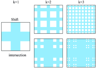
The smallest decay rate, unlike the Weyl law exponent, seems to be very sensitive to the short-time dynamics of the system, as observed in [91]. In this paper two families of baker maps were defined, along with their quantizations, the shift and the intersection families, and for (see left panel of Figure 8). Inside each family, all members have the same Lyapounov exponent and decay rate (and hence the same partial information dimension for their natural measures), but very different short time dynamics. In the intersection family, members have holes that grow with , in such a way that only of all initial conditions remain after the first step. It was observed that the smallest decay rate grows with , so that all resonances have fast decay for large (see right panel of Figure 8). On the other hand, in the shift family the area of the hole is independent of and so is .
6 Eigenvectors
As discussed in Section 3, open quantum propagators are not unitary matrices and their left and right eigenvectors are different,
| (25) |
Just like for closed systems, one would expect on general grounds that in the semiclassical limit these wavefunctions should be related to classical structures. A natural question is the analogue of the quantum ergodicity problem: what are the possible semiclassical limits of Husimi functions of resonance wavefunctions?
The issue of quantum ergodicity for open maps is actually much more difficult than for closed ones, because there are many conditionally invariant measures for any given decay rate, and it is not clear which ones would be more natural as semiclassical limits of Husimi functions.
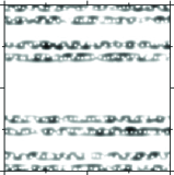
A few general results were obtained in [92]. For example, Husimi functions of right eigenstates, , become concentrated, in the semiclassical limit, on the backward trapped set . This is true in the following sense: suppose a sequence of resonances with increasing , such that the corresponding eigenvalues converge to some value which is different from zero. Then the sequence of (right) Husimi functions will converge to zero at points which do not belong to . We show two illustrative examples in Figure 9. Analogously, left eigenstates concentrate on as . The results in [92] do not indicate how fast the value of goes to zero if , but in [76] it was shown that this happens (at least for the baker map) exponentially fast, i.e. like for some constant .
It is also possible to obtain some semiclassical information about how these Husimi functions are distributed on their support. First, remember that the sets intersect the backward trapped set. Let these regions be semiclassically quantized by phase space projectors (as discussed in [93]). The open propagator thus satisfies . It was shown in [92] that
| (26) |
The left hand side of the above equation measures the weight of on the region , and the right hand side relates this to the decay rate. This relation is tested in Figure 10 for the baker map.
It was first noticed that the functions had fractal signatures of the set in [83]. In this paper it was suggested that, for a sequence of states whose decay rate converges to the classical one, the (right) Husimi functions should converge to the classical equilibrium measure. This would in fact be consistent with the result (26) above, because since and since the area decreases by at each step, we have
| (27) |
However, this convergence has not been proven and numerical evidence is inconclusive. Equation (26) also predicts that states with must show some concentration on the hole and its first pre-images and, conversely, that states with (supersharp) must avoid these sets and localize closer to the invariant set.
This problem was extensively discussed for the baker map in [76]. In particular, this system admits a non-canonical quantization, known as the Walsh quantization, in which it is exactly solvable (unfortunately it is not clear how general are the results proven in this special setting). For example, right Husimi functions having self-similar properties can be explicitly constructed for this system. This was discussed again in a slightly different setting in [94] where, among other things, a kind of quantum unique ergodicity was proven at the edges of the spectrum.
Related to the problem of quantum ergodicity is the phenomenon of quantum scarring. This is a generic name given to concentration of quantum states in the vicinity of periodic orbits. For open systems the question of scarring carries an extra interest, because of the interplay with the decay rate. States with small decay rate must survive in the system for a long time, and it is natural to expect them to be scarred along periodic orbits. States with can show scarring, and this has been observed. But, as discussed in relation with (26), scarring is more likely for (this was also suggested in [82]). Moreover, how the effect behaves in the semiclassical limit is rather unclear. This is connected to the subject of the previous Section, because a gap may develop in the spectrum such that no states with survive the semiclassical limit.
It was observed in [83] that resonances of the kicked rotator with small decay rates were scarred. The subject was taken up again in [73], where the open cat map was studied. A set of quantum states specially suited for studying scarring, the so-called scar functions already available for closed maps [95, 96], was adapted to the open setting in [77, 78], where it was observed that the baker map with low had some resonance wave functions that could be obtained as a superposition of only two of these states. However, it was also suggested in [79] that classical information outside the saddle, such as diffraction effects, must somehow be incorporated if a semiclassical approach is to accurately reproduce resonance wave functions.
In this context, a new phase space representation of resonance states was introduced in [97], which is a generalization of the Husimi function. It is given by
| (28) |
Since is localized on and is localized on , the quantity must be localized on their intersection, the saddle, and may be useful for revealing scarring effects. This was verified for the baker map. It was also noticed that, for finite , the states with large decay rates can have significant values of outside of that fractal set.

A quantity derived from was introduced in [91] as a quantitative measure of localization:
| (29) |
where
| (30) |
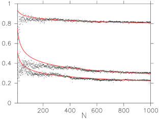
and represents the density matrix of any coherent state. As defined, is equal to for a coherent state (perfect localization) and for a uniformly distributed state in a -dimensional Hilbert space. We see in Figure 11 that the value of behaves rather erratically as a function of the decay rate for individual states. However, a cumulative value , where the sum runs over states with increasing decay rate, shows an almost monotonic behaviour, with smaller decay rates corresponding to stronger localization.
7 Non-ideal escape
A generalization of open systems which has attracted attention recently is the possibility to define holes that are only partially transparent: when a point hits the hole, it has a finite probability of escaping, but may also continue being propagated inside. This may be called non-ideal or refractive escape, because it is supposed to mimic the ray-splitting that takes place at the interface between two media with different indices of refraction. It can also be used to model quantum dots coupled with tunnel barriers or any kind of losses.
Let us suppose a dielectric sample of refractive index , outside of which the refractive index is . When the wavelength is much smaller than the average radius of the sample, we may consider propagation of rays. These follow straight lines, except when they meet the boundary. According to Snell’s law, they then experience specular reflection. This is what is known as a dynamical billiard. It is usual to define boundary coordinates as follows. Choose an arbitrary point at the boundary and let be the distance along the boundary between a collision and . Clearly, , where is the perimeter of the sample. The other coordinate, , is the sine of the angle between the incoming ray and the normal to the boundary at the collision point. It is possible to show that in this coordinate system the dynamics is area-preserving.
The propagation of rays inside the dielectric sample is thus reduced to a discrete map in the variables , of the kind we have been considering. Now we must incorporate the fact that, at each collision, some amount of light is refracted out of the sample. The intensity of the reflected beam is given by Fresnel’s law (for transverse magnetic polarization, for instance):
| (31) |
and depends on the angle of incidence. Refraction does not occur if , which is called the critical angle.
Refraction can be modeled in a chaotic map by assigning an escape probability to each point in phase space [98]. An attempt to be realistic would try to simulate Fresnel’s law. More simply, one can define a finite hole corresponding to and associate to it a constant escape probability. Now it is no longer possible to simply follow initial conditions with time, because one must keep track of probabilities. This can be solved by considering only the evolution of probability densities (this is also discussed in [23]).
We can start with the uniform density in phase space, for example, and let it evolve under the partially open map. Equivalently, we can associate an initial intensity with each point, and this intensity is reduced every time the point falls in the (partially transparent) hole. In particular, the set of points whose intensity remains forever equal to its initial value is nothing but the forward trapped set that would correspond to a totally transparent hole. However, other regions may also have high intensity and be important for long-time properties.
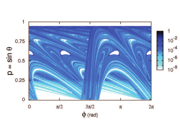
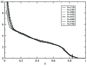
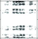
Strictly speaking, the system will have a (conditionally invariant) equilibrium measure whose support (the ‘forward trapped set’) is the entire phase space, since the intensity of a point will never be exactly zero. In other words, will have a trivial Minkowski dimension . However, the intensity after a long time will be a wildly fluctuating quantity and usually there will exist non-trivial dimensions (naturally, the same is true for backward time evolution). Further discussion of these points can be found in [99, 100, 23], along with pictures of such intensities for the stadium, annular and cardioid billiards, respectively. We show an example in Figure 12.
Quantization of partially open maps poses no difficulty. We continue assuming that the hole is a strip (or a union of strips) parallel to one of the axes. Instead of using a projector , one needs only multiply the closed-system propagator by a diagonal matrix whose elements are equal to where the reflection probability is (in principle, the phases of such elements are arbitrary; obviously, we assume ).
The first question one would ask in this setting is about the analogue of the Weyl law. Do we see a fractional exponent in the way the number of resonances scales with ? It was initially suggested in [99] that the Weyl law could be sensitive to the different fractal dimensions present in the classical equilibrium measure. By counting resonances in the dielectric stadium billiard, different exponents in the Weyl law were found depending on the decay rate; moreover, these exponents were in the same range as the numerically determined .
However, it was later proved [101, 102] that in the semiclassical limit the resonances tend to cluster at a particular value of the decay rate. More specifically, let denote the reflection probability at point . In the long run, a typical (ergodic) trajectory will sample all of phase space. At each point, its intensity is multiplied by . This process is additive in the logarithm, resulting in the average decay , where
| (32) |
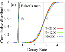
It was shown in [101, 102] that the number of resonances with decay rate inside a fixed interval containing scales with in the semiclassical limit. In other words, most resonances have this decay rate. This result is illustrated in Figure 13. Since the resonances counted in [99] were in a range that contained , the fractional exponents observed are probably due to insufficient statistics or the semiclassical regime not been reached yet.
Another result presented in [101, 102] is that, for strongly chaotic systems, the width of the distribution of decay rates around decays like . This was proven for a toy model and numerically observed (albeit not quite clearly) for the baker map and a perturbed cat map. It is natural to expect that this spectral width should depend on some type of variance of the function . In particular, the width is zero if is constant all over phase space. This point has not been investigated.
The distribution of resonances for partially open maps had already been considered numerically in [98] using the kicked rotator as a model. This paper also suggested a random matrix theory approach (see next Section), which was later tested in [103] for the stadium billiard. Good agreement was obtained, as long as the mean decay rate and the effective number of modes were suitably adjusted.
8 Random matrix theory
An approach which has been very successful in all areas of quantum chaos is the theory of random matrices [107]. In essence, the specific relevant operator (Hamiltonian, matrix, propagator) is abandoned and replaced by a random matrix, i.e. only statistical properties are studied with respect to a certain ensemble of matrices. How this ensemble is chosen is dictated by the situation at hand. Approaches based on random matrices exist for several areas of physics, including the quantum mechanics of closed chaotic systems [108] and chaotic transport [29]. Many examples can be found in a recent Handbook [109].
To replace the Hamiltonian of a closed system, for example, it is important that hermitian matrices be used. The simplest possibility is then to replace the matrix elements with identically distributed Gaussian random variables, while respecting the hermiticity constraint. This gives rise to the Gaussian Unitary Ensemble (it is called Unitary because it is invariant under unitary transformations). If there is time-reversal symmetry, the Hamiltonian can be made real without diagonalization. What is needed then is an ensemble of real symmetric matrices, and this leads to the Gaussian Orthogonal Ensemble. It is common practice to associate an index with complex matrices and with real matrices (this is sometimes called the Dyson parameter). Gaussian ensembles were recently reviewed in [110].
8.1 Effective Hamiltonian approach
It is possible to model scattering by writing the matrix as , where is a coupling matrix between the system and the outside and is an effective non-hermitian Hamiltonian. The poles of are then the eigenvalues of . This is sometimes called the Heidelberg approach. Assuming energy-independence of the coupling elements and neglecting direct processes, this latter matrix can be taken as , and considered as being uniformly distributed in one of the Gaussian ensembles. The reader can consult [112, 113, 114, 24, 25] for further information.
Different regimes can be studied depending on coupling strength and the interplay between and . The limit is always intended. The number of channels may remain fixed, in which case the hole is not classical in size. For small coupling, all eigenvalues acquire small imaginary parts (smaller than the mean level spacing). For large coupling, the phenomenon of resonance trapping occurs [115]: only a few resonances acquire large imaginary parts, while most of them approach the real axis.
The case of classical opening, closer in spirit to the subject of this review, corresponds to keeping the ratio fixed as . This corresponds to the size of the hole, . As we have seen, it makes sense to consider this as a small variable. It can be shown [116, 117] that in this case the density of resonances exhibits a gap: it vanishes for decay rates smaller than , which can be identified with the classical decay rate. Moreover, this density decays like for .
8.2 Approach via truncations
The propagator of a closed quantum map is a -dimensional unitary matrix, . If there is time-reversal symmetry, this matrix is also symmetric. These are the only constraints that must be imposed. The ensemble of random unitary matrices is nothing but the unitary group equipped with its unique invariant (probability) measure, the Haar measure. In this context, this ensemble is called the Circular Unitary Ensemble, the CUE. If symmetry is imposed, , we obtain the Circular Orthogonal Ensemble, the COE.
The propagator of an open quantum map is obtained by multiplying the closed propagator by a projector. This is sometimes called a truncation: some columns of are set equal to zero to produce . Therefore, it is natural to take as being uniformly distributed in the CUE and introduce an ensemble of truncated unitary matrices (TCUE). This was done in [111].
We therefore have -dimensional unitary matrices truncated by multiplying from the right by a projector. Let the kernel of the projector have dimension , as before, and let be the number of eigenvalues that are not identically zero. Just like for the effective hamiltonian approach, in the ‘semiclassical’ limit there are two choices for the behaviour of the truncation: the kernel dimension can remain fixed in order to model ‘quantum’ holes, or we can have with fixed in order to model ‘classical’ holes.
Since any element of the TCUE is subunitary, the spectrum always lies inside the unit disk in the complex plane. The joint probability density of the eigenvalues can be exactly obtained. For large , the original ensemble of is not relevant, i.e. results are the same for both unitary and orthogonal classes. Apparently, the presence of the hole is enough to effectively break symmetry. The probability distribution of the modulus squared of the eigenvalues can also be found. Using the quantity mentioned above, the distribution of is given by
| (33) |
if and vanishes otherwise.
Since is the area of the complement of the hole, it is natural to interpret it in terms of a fictitious decay rate as . Therefore, this approach also predicts a spectral gap in the limit , so that states with become increasingly rare. Note however that the interpretation of as a decay rate is not so straightforward for discrete time systems (maps), e.g.
| (34) |
If we were to interpret as a decay rate, then according to (33) its density decays quadratically, in agreement with the effective Hamiltonian approach.
In Figure 14 the prediction (33) is checked for the open kicked rotator [not available in the Arxiv version]; good agreement is found, provided the dimension is renormalized according to the fractal Weyl law.
Notice that this approach is not able to give any insight into the fractal Weyl law itself, since this is obviously a system-specific feature, i.e. it depends on details of the dynamics. One way to see this is that although it is possible to build the escape rate into random matrix theory, simply using the size of the hole, the same is not true for the Lyapounov exponent (in a sense, this quantity is ‘infinite’ in this theory).
Even though they are suppressed in the limit, we can ask about statistics of resonances inside the gap, the supersharp ones. For example, we can consider states with , with . These will approach the maximum value from above in the semiclassical limit. It turns out that they have a finite density function proportional to , where erfc is the complementary error function [118]. Another interesting question is the distribution of the smallest decay rate . Equivalently, we can consider the largest eigenvalue modulus squared, . It was shown in [119, 84] that the modified variable satisfies a Gumbel distribution as .
8.3 Eigenvectors
A different line of investigations would be to consider statistics of the eigenvectors. Usually, the quantity
| (35) |
is considered (see, for example, [120, 121]). This is called eigenvector correlator or Petermann factor, and is related to the line width of the lasing mode in open resonators. Results of this type were reviewed in [113]. This can be generalized to an off-diagonal version , which was shown in [122] to be related to the statistics of resonance width shifts under external perturbations.
Another type of quantity,
| (36) |
where is the th component of a right eigenvector, was considered in [123, 124].
Research along this line has always been done within the effective Hamiltonian approach, in the case when the number of states in the hole is much smaller than total number of states, . To the knowledge of this author, there are no works about statistics of eigenvectors for classical holes or truncated unitary matrices.
8.4 Non-ideal escape
The case of non-ideal escape can also be treated in two ways, using effective Hamiltonians or opening propagators. Within the first approach the finite transparencies of the decay channels are incorporated into the coupling matrix . When all channels are equivalent the degree of resonance overlapping is controlled by the parameter [125] where is the transparency and is the number of channels.
The propagator of partially open systems should be modeled as , where is a fixed diagonal matrix with nonnegative entries representing reflection probabilities and is uniformly distributed in a circular ensemble. This was first considered in [98], with in the COE, but only numerical results (for distribution of decay rates and eigenvectors) were presented. Later, the exact density of states with in the CUE was derived in [126]. Its asymptotic behaviour as , obtained in [127, 128], is as follows: if denotes eigenvalue modulus, its cumulative distribution is implicitly defined by
| (37) |
where is
| (38) |
In particular, in the semiclassical limit the eigenvalues of lie inside an annulus in the complex plane: their modulus squared must be larger than the arithmetic mean of the eigenvalues of and smaller than their harmonic mean.
9 Some open problems
The topic of resonances is of wide interest, both theoretically and experimentally. There is a variety of settings, motivations, applications, approaches, etc. that make it impossible to provide a truly comprehensive review. We have focused on quantum maps, with chaotic classical dynamics and classical openings. We hope to have touched upon some of the more interesting points that have recently attracted attention and to have provided some references for the interested reader.
We conclude this review with a few open problems. These are more general indications of interest than specific questions. It is likely that as these matters are investigated further other interesting problems will come to the front.
For systems with ballistic escape, we would like to mention the following points:
-
•
Exponent in the fractal Weyl law. A rigorous proof of this, aside from the non-generic Walsh quantization of the baker map, is still lacking. Heuristic understanding has been achieved from different points of view, however, and such proof is likely to be extremely technical.
-
•
Prefactor in the fractal Weyl law. Does the profile function of the resonance spectrum have anything to do with classical dynamics? The random matrix theory prediction works well for the kicked rotator, but not for the baker map. Can this be understood?
The next points apply to ballistic escape, but also make sense for systems with non-ideal escape:
-
•
Spectral gap. Under what conditions is it true that as there are no resonances in a certain region? What exactly is the Weyl law for supersharp resonances?
-
•
Quantum ergodicity. What are the possible semiclassical limits for Husimi functions with a given decay rate? Do they have self-similar properties? Is there a preferred classical eigenmeasure?
-
•
Scarring. How does the scarring by periodic orbits behaves in the semiclassical limit? Is the amount of scarring related to the decay rate? Are supersharp resonances special in this respect?
-
•
Semiclassical approach. It seems that in order to reproduce resonance wave functions it is necessary to include more information than just periodic orbits (maybe diffraction). It is not clear how to proceed in this direction.
-
•
Statistics of eigenvectors. Virtually nothing is known in the case of classical openings, even within random matrix theory.
References
References
- [1]
- [2] S. Oberholzer, E.V. Sukhorukov and C. Schönenberger, Nature 415, 765 (2002).
- [3] W. Lu, Z. Ji, L. Pfeiffer, K.W. West and A.J. Rimberg, Nature 423, 422 (2003).
- [4] J. Bylander, T. Duty and P. Delsing, Nature 434, 361 (2005).
- [5] E.V. Sukhorukov, A.N. Jordan, S. Gustavsson, R. Leturcq, T. Ihn and K. Ensslin, Nature Phys. 3, 243 (2007).
- [6] F. Miao, S. Wijeratne, Y. Zhang, U.C. Coskun, W. Bao and C.N. Lau, Science 317, 1530 (2007).
- [7] L. A. Ponomarenko, F. Schedin, M.I. Katsnelson, R. Yang, E.W. Hill, K.S. Novoselov and A.K. Geim, Science 320, 356 (2008).
- [8] C. Stampfer, J. Güttinger, S. Hellmüller, F. Molitor, K. Ensslin and T. Ihn, Phys. Rev. Lett. 102, 056403 (2009).
- [9] B. Dietz, T. Friedrich, H.L. Harney, M. Miski-Oglu, A. Richter, F. Schäfer, and H.A. Weidenmüller, Phys. Rev. E 81, 036205 (2010).
- [10] R. Schäfer, H-J. Stockmann, T. Gorin and T.H. Seligman, Phys. Rev. Lett. 95, 184102 (2005).
- [11] A. Backer, R. Ketzmerick, S. Löck, M. Robnik, G. Vidmar, R. Höhmann, U. Kuhl and H.-J. Stöckmann, Phys. Rev. Lett. 100, 174103 (2008).
- [12] B. Dietz, A. Heine, A. Richter, O. Bohigas and P. Leboeuf, Phys. Rev. E 73, 035201(R) (2006).
- [13] F.B. Bateman, S.M. Grimes, N. Boukharouba, V. Mishra, C.E. Brient, R.S. Pedroni, T.N. Massey and R.C. Haight, Phys. Rev. C 55, 133 (1997).
- [14] J. Carter, H. Diesener, U. Helm, G. Herbert, P. von Neumann-Cosel, A. Richter, G. Schrieder and S. Strauch, Nucl. Phys. A 696, 317 (2001).
- [15] M. Wright and R. Weaver (Eds.), New Directions in Linear Acoustics (Cambridge University Press, 2010).
- [16] C. Gmachl, F. Capasso, E.E. Narimanov, J.U. Nöckel, A.D. Stone, J. Faist, D.L. Sivco and A.Y. Cho, Science 231, 486 (1998).
- [17] S.-Y. Lee, S. Rim, J.-W. Ryu, T.-Y. Kwon, M. Choi and C.-M. Kim, Phys. Rev. Lett. 93, 164102 (2004).
- [18] T. Tanaka, M. Hentschel, T. Fukushima and T. Harayama, Phys. Rev. Lett. 98, 033902 (2007).
- [19] I. Rotter, J. Phys. A 42, 153001 (2009).
- [20] R. de la Madrid and M. Gadella, Am. J. Phys. 70, 626 (2002).
- [21] A. Bohm and M. Gadella, Lecture Notes in Physics 348 (Springer, 1989).
- [22] C.P. Dettmann, arXiv:1007.4166v1 [nlin.CD].
- [23] E. Altmann, J.S.E. Portela and T. Tél, arXiv:1208.0254 [nlin.CD].
- [24] Y.V. Fyodorov and D.V. Savin, Chapter 34 of [109].
- [25] G.E. Mitchell, A. Richter and H.A. Weidenmüller, Rev. Mod. Phys. 82, 2845 (2010).
- [26] S. Nonnenmacher, Nonlinearity 24, R123 (2011).
- [27] Y. Imry and R. Landauer, Rev. Mod. Phys. 71, S306 (1999).
- [28] D. Waltner, Semiclassical Approach to Mesoscopic Systems (Springer, 2012).
- [29] C.W.J. Beenakker, Rev. Mod. Phys. 69, 731 (1997).
- [30] J.R. Dorfman, An Introduction to Chaos in Nonequilibrium Statistical Mechanics (Cambridge University Press, 1999).
- [31] E. Ott, Chaos in Dynamical Systems (Cambridge University Press, 2002).
- [32] Y.C. Lai and T. Tél, Transient Chaos: Complex Dynamics in Finite Time Scales (Springer, 2011).
- [33] S. Nonnenmacher and M. Zworski, J. Phys. A 38, 10683 (2005).
- [34] M. Demers and L.S. Young, Nonlinearity 19, 377 (2006).
- [35] V. Paar and N. Pavin, Phys. Rev. E 55, 4112 (1997).
- [36] E.G. Altmann, E.C. da Silva and I.L. Caldas, Chaos 14, 975 (2004).
- [37] L. Bunimovich and A. Yurchenko, Israel J. Math. 182, 229 (2011).
- [38] J.M. Pedrosa, G.G. Carlo, D.A. Wisniacki and L. Ermann, Phys. Rev. E 79, 016215 (2009).
- [39] G. Pianigiani and J. Yorke, Trans. Amer. Math. Soc. 252, 351 (1979).
- [40] H. Kantz and P. Grassberger, Physica D 17, 75 (1985).
- [41] J.P. Gazeau, Coherent States in Quantum Physics (John Wiley & Sons, 2009).
- [42] M. Saraceno, Ann. Phys. 199, 37 (1990).
- [43] H. Schomerus and Ph. Jacquod, J. Phys. A 38, 10663 (2005).
- [44] N.L. Balazs and A. Voros, Ann. Phys., N.Y. 190, 1 (1989).
- [45] J. H. Hannay, M. V. Berry, Physica D 1 267 (1980).
- [46] B. Eckhardt, J. Phys. A: Math. Gen. 19, 1823 (1986).
- [47] J.P. Keating, Nonlinearity 4, 309 (1991).
- [48] G. Casati, B.V. Chirikov, J. Ford and F.M. Izrailev, Lect. Notes Phys. 93, 334 (1979).
- [49] F.M. Izrailev, Phys. Rep. 196, 299 (1990).
- [50] J.H. Hannay, J.P. Keating and A.M. Ozorio de Almeida, Nonlinearity 7, 1327 (1994).
- [51] T. Brun and R. Schack. Phys. Rev. A 59, 2649 (1999).
- [52] F.L. Moore, J.C. Robinson, C.F. Bharucha, B. Sundaram and M.G. Raizen, Phys. Rev. Lett. 75, 4598 (1995).
- [53] H. Ammann, R. Gray, I. Shvarchuck and N. Christensen, Phys. Rev. Lett. 80, 4111 (1998).
- [54] E.J. Heller, Phys. Rev. Lett. 53, 1515 (1984).
- [55] F. Faure, S. Nonnenmacher and S. De Bievre, Commun. Math. Phys. 239, 449 (2003).
- [56] N. Anantharaman and S. Nonnenmacher, Ann. Henri Poincaré 8, 37 (2007).
- [57] M.D. Esposti, S. Graffi and S. Isola, Comm. Math. Phys. 167, 471 (1995).
- [58] A. Bouzouina and S. De Bièvre, Commun. Math. Phys. 178 83 (1996).
- [59] P. Kurlberg and Z. Rudnick, Commun. Math. Phys. 222, 201 (2001).
- [60] M. Degli Esposti, S. Nonnenmacher and B. Winn, Commun. Math. Phys. 263 325 (2006).
- [61] S. Nonnenmacher, arXiv:1005.5598v2 [math.DS].
- [62] M. Brack and R. Bhaduri, Semiclassical Physics (Westview Press, 2008).
- [63] K. Lin, J. Comput. Phys. 176, 295 (2002).
- [64] K. Lin and M. Zworski, Chem. Phys. Lett. 355, 201 (2002).
- [65] W.T. Lu, S. Sridhar and M. Zworski, Phys. Rev. Lett. 91, 154101 (2003).
- [66] A. Eberspächer, J. Main, and G. Wunner, Phys. Rev. E 82, 046201 (2010).
- [67] J.A. Ramilowski, S.D. Prado, F. Borondo and D. Farrelly, Phys. Rev. E 80, 055201(R) (2009).
- [68] J. Sjöstrand, Duke Math. J. 60, 1 (1990).
- [69] J. Sjöstrand and M. Zworski, Duke Math. J. 137, 381 (2007).
- [70] S. Nonnenmacher and M. Zworski, Commun. Math. Phys. 269, 311 (2007).
- [71] H. Schomerus and J. Tworzydło, Phys. Rev. Lett. 93 154102 (2004).
- [72] D.L. Shepelyansky, Phys. Rev. E 77, 015202(R) (2008).
- [73] D. Wisniacki and G.G. Carlo, Phys. Rev. E 77, 045201(R) (2008).
- [74] S. Nonnenmacher, J. Sjöstrand and M. Zworski, arXiv:1105.3128v1 [math.AP].
- [75] M. Kopp and H. Schomerus, Phys. Rev. E 81, 026208 (2010).
- [76] S. Nonnenmacher and M. Rubin, Nonlinearity 20, 1387 (2007).
- [77] M. Novaes, J.M. Pedrosa, D. Wisniacki, G.G. Carlo and J.P. Keating, Phys. Rev. E 80, 035202(R) (2009).
- [78] J.M. Pedrosa, D. Wisniacki, G.G. Carlo and M. Novaes, Phys. Rev. E 85, 036203 (2012).
- [79] G.G. Carlo, D.A. Wisniacki, L. Ermann, R.M. Benito and F. Borondo, arXiv:1207.5785v1 [quant-ph].
- [80] A. Ishii, A. Akaishi, A. Shudo and H. Schomerus, Phys. Rev. E 85, 046203 (2012).
- [81] J.M. Pedrosa, G.G. Carlo, D. Wisniacki and L. Ermann, Phys. Rev. E 79, 016215 (2009).
- [82] F. Borgonovi, I. Guarneri and D.L. Shepelyansky, Phys. Rev. A 43, 4517 (1991).
- [83] G. Casati, G. Maspero and D.L. Shepelyansky, Physica D 131 311 (1999).
- [84] M. Novaes, Phys. Rev. E 85, 036202 (2012).
- [85] P. Gaspard and S.A. Rice, J. Chem. Phys. 90, 2242 (1989).
- [86] A. Wirzba, Phys. Rep. 309, 1 (1999).
- [87] P. Gaspard, Chaos, Scattering and Statistical Mechanics (Cambridge University Press, 2005).
- [88] S. Nonnenmacher and M. Zworski, Acta Math. 203, 149 (2009).
- [89] D. Jakobson and F Naud, arXiv:1011.6264v1 [math.SP].
- [90] F. Naud, arXiv:1203.4378v1 [math.SP].
- [91] L. Ermann, G.G. Carlo, J.M. Pedrosa and M. Saraceno, Phys. Rev. E 85, 066204 (2012).
- [92] J.P. Keating, M. Novaes, S.D. Prado and M. Sieber, Phys. Rev. Lett. 97, 150406 (2006).
- [93] R.O. Vallejos and M. Saraceno, J. Phys. A 32, 7273 (1999).
- [94] J.P. Keating, S. Nonnenmacher, M. Novaes and M. Sieber, Nonlinearity 21, 2591 (2008).
- [95] E.G Vergini, D. Schneider and A.M.F. Rivas, J. Phys. A 41, 405102 (2008).
- [96] L. Ermann and M. Saraceno, Phys. Rev. E 78, 036221 (2008).
- [97] L. Ermann, G.G. Carlo and M. Saraceno, Phys. Rev. Lett. 103, 054102 (2009).
- [98] J.P. Keating, M. Novaes and H. Schomerus, Phys. Rev. A 77, 013834 (2008).
- [99] J. Wiersig and J. Main, Phys. Rev. E 77, 036205 (2008).
- [100] E. Altmann, Phys. Rev. A 79, 013830 (2009).
- [101] S. Nonnenmacher and E. Schenck, Phys. Rev. E 78, 045202(R) (2008).
- [102] E. Schenck, Ann. Henri Poincaré 10, 711 (2009).
- [103] H. Schomerus, J. Wiersig and J. Main, Phys. Rev. A 79, 053806 (2009).
- [104] M. Asch and G. Lebeau, Experimental Math. 12, 227 (2003).
- [105] G. Riviere, arXiv:1109.1909v2 [math-ph].
- [106] G. Riviere, arXiv:1202.5123v2 [math.AP].
- [107] M.L. Mehta, Random Matrices (Academic Press, 2004).
- [108] F. Haake, Quantum Signatures of Chaos (Springer, 2001).
- [109] G. Akemann, J. Baik and P. Di Francesco (Ed.),The Oxford Handbook of Random Matrix Theory (Oxford University Press, 2011).
- [110] H.A. Weidenmüller and G.E. Mitchell, Rev. Mod. Phys. 81, 539 (2010).
- [111] K. Życzkowski and H.-J. Sommers, J. Phys. A 33, 2045 (2000).
- [112] Y.V. Fyodorov and H.-J. Sommers, J. Math. Phys. 38, 1918 (1997).
- [113] Y.V. Fyodorov and H.-J. Sommers, J. Phys. A 36, 3303 (2005).
- [114] Y.V. Fyodorov, D.V. Savin and H.-J. Sommers, J. Phys. A 38, 10731 (2005).
- [115] V.V. Sokolov and V.G. Zelevinsky, Nucl. Phys. A 504, 562 (1989).
- [116] F. Haake, F. Izrailev, N. Lehmann, D. Saher and H.-J. Sommers, Z. Phys. B 88, 359 (1992).
- [117] N. Lehmann, D. Saher, V.V. Sokolov and H.-J. Sommers, Nucl. Phys. A 582, 223 (1995).
- [118] B.A. Khoruzhenko and H.-J. Sommers, Chapter 18 of [109].
- [119] B. Rider, J. Phys. A 36, 3401 (2003).
- [120] H. Schomerus, K.M. Frahm, M. Patra and C.W.J. Beenakker, Physica A 278, 469 (2000).
- [121] B. Mehlig and M. Santer, Phys. Rev. E 63, 020105(R) (2001).
- [122] Y. Fyodorov and D.V. Savin, Phys. Rev. Lett. 108, 184101 (2012).
- [123] C. Poli, D. V. Savin, O. Legrand and F. Mortessagne, Phys. Rev. E 80, 046203 (2009).
- [124] D.V. Savin, O. Legrand and F. Mortessagne, Europhys. Lett. 76, 774 (2006).
- [125] D.V. Savin and V.V. Sokolov, Phys. Rev. E 56, R4911 (1997).
- [126] Y. Wei and Y.V. Fyodorov, J. Phys. A 41, 502001 (2008).
- [127] U. Haagerup and F. Larsen, J. Funct. Anal. 176, 331 (2000).
- [128] E. Bogomolny, J. Phys. A 43, 335102 (2010).