Shape evolution and the role of intruder configurations in Hg isotopes within the interacting boson model based on a Gogny energy density functional

Abstract

The interacting boson model with configuration mixing, with parameters derived from the self-consistent mean-field calculation employing the microscopic Gogny energy density functional, is applied to the systematic analysis of the low-lying structure in Hg isotopes. Excitation energies, electromagnetic transition rates, deformation properties, and ground-state properties of the ^172-204Hg nuclei are obtained by mapping the microscopic deformation energy surface onto the equivalent IBM Hamiltonian in the boson condensate. These results point to the overall systematic trend of the transition from the near spherical vibrational state in lower-mass Hg nuclei close to ¹⁷²Hg, onset of intruder prolate configuration as well as the manifest prolate-oblate shape coexistence around the mid-shell nucleus ¹⁸⁴Hg, weakly oblate deformed structure beyond ¹⁹⁰Hg up to the spherical vibrational structure toward the near semi-magic nucleus ²⁰⁴Hg, as observed experimentally. The quality of the present method in the description of the complex shape dynamics in Hg isotopes is examined.

I Introduction

Both shape transition and shape coexistence in finite nuclei have been a theme of major interests in the field of low-energy nuclear structure study. In particular, significantly low-lying excited $0^{+}$ states close in energy to the $0^{+}$ ground-state have been observed in some nuclei, that reveal the coexistence of different intrinsic shapes. Numerous efforts have already been made to better understand the nature of such stunning shape phenomena from both the theoretical and experimental sides (see Refs. Heyde et al. (1983); Wood et al. (1992); Andreyev et al. (2000); Julin et al. (2001); Heyde and Wood (2011) for review).

In terms of the nuclear shell model Federman and Pittel (1977); Van Duppen et al. (1984); Heyde et al. (1985, 1987); Heyde and Meyer (1988); Heyde et al. (1995), the emergence of low-lying excited $0^{+}$ states can be traced back to multiparticle-multihole excitations. This scenario applies to the neutron-deficient nuclei in the Lead region with $Z\approx 82$. In this case, two or four protons are excited from the $Z=50-82$ major shell across the $Z=82$ closed shell to the $h_{9/2}$ orbit. The residual interaction between the valence protons and neutrons becomes subsequently enhanced, leading to the lowering of the excited $0^{+}$ energies. This effect is most significant around the neutron mid-shell $N=104$.

From the experimental side, extensive $\gamma$-ray spectroscopic studies have opened up a vast opportunity to extend the knowledge of the precise low-lying structure of neutron-deficient Hg isotopes (cf. Julin et al. (2001); Heyde and Wood (2011) for review). As observed Julin et al. (2001), the second $0^{+}$ energy level becomes noticeably lower as a function of the neutron number, starting from around the ¹⁸⁸Hg down to the middle of the major shell $N=104$. This $0^{+}_{2}$ excited state reaches a minimum in energy around ¹⁸²Hg and then goes up from ¹⁸⁰Hg to ¹⁷⁸Hg Elseviers et al. (2011). The energy levels of the yrast $2^{+}$, $4^{+}$ and $6^{+}$ states become much higher in ^172,174,176Hg, suggesting the transition to spherical vibrational states Julin et al. (2001). This picture is quite vividly observed in the parabolic trend of the states, which may belong to the band built on the low-lying excited $0^{+}$ state, as functions of the neutron number in the Hg chain. On the other hand, from around ¹⁹²Hg to the heavier isotopes, the observed energy levels of the yrast band remain almost constant toward the $N=126$ closed shell and form the deformed rotational band Brookhaven National Nuclear Data Center . Given the recent advances in the experimental studies, it is quite timely, as well as significant, to address, through a theoretical description of the relevant spectroscopy comparable to the experiments, the important issues of the origin of the low-lying excited $0^{+}$ state and the corresponding shape dynamics in the neutron-deficient Hg isotopes.

Let us stress, that these heavy mass systems are currently beyond the reach of large-scale shell-model studies with a realistic configuration space and nucleon-nucleon interaction. Therefore a drastic truncation scheme is required to make the problem more feasible. Such a framework is provided by the interacting boson model (IBM) Iachello and Arima (1987), which employs the monopole $s$ and quadrupole $d$ bosons, associated to the $J^{\pi}=0^{+}$ and $2^{+}$ collective pairs of valence nucleons, respectively Arima et al. (1977); Otsuka et al. (1978a, b). The collective levels and the transition rates are generated by the diagonalization of the boson Hamiltonian composed of only a few essential interaction terms. To handle the configuration mixing in the IBM framework, Duval and Barrett proposed to extend the boson Hilbert space to the direct sum of the configuration sub-spaces corresponding to the $2np$-$2nh$ excitation ($n=0,1,2\ldots$) that comprises $N_{B}+2n$ bosons Duval and Barrett (1981). Various features relevant to the shape coexistence phenomena in the Pb region have been investigated within the IBM configuration mixing model: the empirical collective structures from Po down to Pt isotopes Duval and Barrett (1982); Barfield et al. (1983); De Coster et al. (1999); Fossion et al. (2003); García-Ramos et al. (2011), geometry and phases Frank et al. (2004, 2006); Irving Morales et al. (2008), and the algebraic features (in terms of the so called intruder spin) Heyde et al. (1992); De Coster et al. (1996); Lehmann et al. (1997). Nevertheless, one of the main difficulties was that, since too many parameters are involved in this prescription, one has to specify the form of the model Hamiltonian rather a priori and/or simply select the parameters by the fit to available data.

On the other hand, the energy density functional (EDF) framework has been successful in the self-consistent mean-field study of bulk nuclear properties and collective excitations Bender et al. (2003) with various classes of effective interactions, e.g., Skyrme Skyrme (1958); Vautherin and Brink (1972), Gogny J. Decharge and M. Girod and D. Gogny (1975), and those used within relativistic mean-field (RMF) models Vretenar et al. (2005); Nikšić et al. (2011). The mean-field approximation provides the coexisting minima in the deformation energy surface, which are associated to the different intrinsic geometrical shapes Nazarewicz (1993). Deformation properties and collective excitations, relevant to the shape coexistence in the neutron-deficient Pb and Hg isotopes, have been investigated using Skyrme Duguet et al. (2003); Bender et al. (2004), Gogny Girod and Reinhard (1982); Delaroche et al. (1994); Chasman et al. (2001); Rodríguez-Guzmán et al. (2004); Egido et al. (2004); Moreno et al. (2006) and the RMF interactions Nikšić et al. (2002) as well as within the Nilsson-Strutinsky method Bengtsson and Nazarewicz (1989); Nazarewicz (1993). Recently, a systematic study of the low-lying states in the Lead region has been performed within the number and angular-momentum projected generator coordinate method with axial symmetry, employing the Skyrme EDF Yao et al. (2013).

A method of deriving the IBM Hamiltonian by combining the density functional framework with the IBM has been developed in Ref.Nomura et al. (2008). Within this method, excitation energies and transition rates are calculated by mapping the deformation energy surface, obtained from the self-consistent mean-field calculation with a given EDF, onto the equivalent IBM Hamiltonian in the boson condensate. This idea has been applied to the mixing of several multiparticle-multihole configurations in Lead isotopes Nomura et al. (2012a) on the basis of the Duval-Barrett’s technique.

In this paper, we apply the above methodology of deriving the configuration mixing IBM-2 Hamiltonian parameters from the microscopic Gogny-EDF quantities to the systematic analysis of low-lying states in a number of Hg isotopes with mass $A=172-204$, with the focus being on the relevant spectroscopy related to the coexistence of different intrinsic shapes around the mid-shell nucleus ¹⁸⁴Hg. The optimal choice of the configuration mixing IBM Hamiltonian consistent with the EDF-based calculations is identified, and the quality of the procedure to extract configuration mixing IBM Hamiltonian is addressed. We shall use the parametrization D1M of the Gogny-EDF Goriely et al. (2009), that has been shown (see, for instance Rodríguez-Guzmán et al. (2010a, b, c)) to have a similar predictive power in the description of nuclear structure phenomena as the more conventional D1S Berger et al. (1984) parameter set. Therefore, another motivation of this work is to test the validity of the new parametrization D1M to the nuclei in Lead region.

This paper is organized as follows: our theoretical framework is briefly summarized in Sec. II. We then show the microscopic (i.e., EDF) and the mapped energy surfaces in the considered Hg isotopes in Sec.III, followed by the systematic calculations, including the energy levels, deformation properties (spectroscopic quadrupole moment and the transition quadrupole moment), and the ground-state properties (mean square charge radii and binding energies) in Sec. IV. The detailed spectroscopy of selected nuclei exhibiting shape coexistence is discussed in Sec. IV whereas Section V is devoted to the concluding remarks. Finally, in appendix A the mapping procedure is described in detail.

II Framework

We first perform a set of constrained Hartree-Fock-Bogoliubov (HFB) calculations using the Gogny-D1M Goriely et al. (2009) EDF to obtain the corresponding mean-field total energy surface in terms of the geometrical quadrupole collective variables $q=(\beta,\gamma)$ Bohr and Mottelsson (1975). Note that the energy surface in this context denotes the total mean-field energy as a function of the deformation variables $q$, where neither the mass parameter nor the collective potential is considered explicitly. In fact, we only consider the symmetry-unprojected HFB energy surface and do not include any zero-point energy corrections. Having the Gogny HFB energy surface, we subsequently map it onto the corresponding IBM energy surface, as described below.

Turning now to the IBM system, in order to treat the proton cross-shell excitation, we shall use the proton-neutron IBM (IBM-2) because it is more realistic than the original version of the IBM (IBM-1), which does not distinguish between proton and neutron degrees of freedom. The IBM-2 comprises neutron (proton) $s_{\nu}$ ($s_{\pi}$) and $d_{\nu}$ ($d_{\pi}$) bosons, which reflect the collective pairs of valence neutrons (protons) Otsuka et al. (1978b). The number of neutron (proton) bosons, denoted as $N_{\nu}$ ($N_{\pi}$), equals half the number of the valence neutrons (protons). The doubly-magic nuclei ¹⁶⁴Pb and ²⁰⁸Pb are taken as the boson vacua (inert cores). As we show below, the Gogny-D1M energy surface exhibits two minima in ^176-190Hg and therefore up to $2p$-$2h$ proton excitations are taken into account to describe these nuclei. For the others, i.e., ^172,174Hg and ^192-204Hg, the corresponding energy surfaces exhibit a single mean-field minimum, which is supposed to be described by a single configuration. Therefore, for the nuclei ^176-190Hg, $N_{\pi}$ is fixed, $N_{\pi}=1$ and 3 for the $0p$-$0h$ and the $2p$-$2h$ configurations, respectively, while $N_{\nu}$ varies between 8 and 11. On the other hand, for the nuclei ^172,174Hg and ^192-204Hg, $N_{\pi}=1$ and $N_{\nu}$ varies between 5 and 6 and between 1 and 7, respectively.

The IBM Hamiltonian of the system, comprising the normal $0p$-$0h$ and the $2p$-$2h$ configurations, is written as Duval and Barrett (1981, 1982)

$$\hat{H}={\cal\hat{P}}_{1}\hat{H}_{1}{\cal\hat{P}}_{1}+{\cal\hat{P}}_{3}(\hat{H}_{3}+\Delta_{intr}){\cal\hat{P}}_{3}+\hat{H}_{mix},$$ (1)

where ${\cal\hat{P}}_{i}$ ($i=1,3$) stands for the projection operator onto the $N_{\pi}=i$ configuration space. The operator $\hat{H}_{i}$ is the Hamiltonian for the configuration with $N_{\pi}=i$ bosons

$$\hat{H}_{i}=\epsilon_{i}\hat{n}_{d}+\kappa_{i}\hat{Q}_{\nu}^{\chi_{\nu,i}}\cdot\hat{Q}_{\pi}^{\chi_{\pi,i}}+\kappa^{\prime}_{i}\hat{L}\cdot\hat{L}+\sum_{\rho^{\prime}\neq\rho}\hat{V}_{\rho\rho\rho^{\prime}},$$ (2)

where the first term $\hat{n}_{d}=\sum_{\rho}d^{\dagger}_{\rho}\cdot d_{\rho}$ ($\rho=\nu$ or $\pi$) stands for the $d$-boson number operator. The second term in Eq. (2) represents the quadrupole-quadrupole interaction between the proton and neutron bosons with $\hat{Q}_{\rho,i}^{\chi_{\rho,i}}=d^{\dagger}_{\rho}s_{\rho}+s^{\dagger}_{\rho}\tilde{d}_{\rho}+\chi_{\rho,i}[d_{\rho}^{\dagger}\times\tilde{d}_{\rho}]^{(2)}$ being the quadrupole operator. The sign of the sum $\chi_{\nu,i}+\chi_{\pi,i}$ specifies whether a given nucleus is prolate or oblate deformed. The third term is relevant for rotationally deformed systems, with $\hat{L}=\sqrt{10}\sum_{\rho}[d^{\dagger}_{\rho}\times\tilde{d}_{\rho}]^{(1)}$ being the boson angular momentum operator. The fourth term on the right-hand side (RHS) of Eq. (2) stands for the three-body (cubic) boson term between the proton and neutron bosons

$$\hat{V}_{\rho\rho\rho^{\prime}}=\sum_{L}\kappa^{\prime\prime(L)}_{\rho\rho\rho^{\prime},i}[d^{\dagger}_{\rho}\times d^{\dagger}_{\rho}\times d_{\rho^{\prime}}^{\dagger}]^{(L)}\cdot[\tilde{d}_{\rho^{\prime}}\times\tilde{d}_{\rho}\times\tilde{d}_{\rho}]^{(L)},$$ (3)

which is identified with the one used in Ref. Nomura et al. (2012b). For each $\rho=\nu$ and $\pi$, there are five linearly independent combinations in Eq. (3), identified by the values $L=0,2,3,4$ and 6. In the present study, as in Ref.Nomura et al. (2012b), we only consider the $L=3$ term, because its classical limit is proportional to $\cos^{2}{3\gamma}$ the only term giving rise to a stable triaxial minimum at $\gamma\approx 30^{\circ}$ Nomura et al. (2012b). The three-body interaction has been restricted to act only between neutrons and protons since such proton-neutron correlation becomes more significant in medium-heavy and heavy nuclei. We have assumed $\kappa^{\prime\prime(3)}_{\pi\pi\nu,i}=\kappa^{\prime\prime(3)}_{\pi\nu\nu,i}\equiv\kappa^{\prime\prime}_{i}$, for simplicity Nomura et al. (2012b).

In Eq. (1), $\Delta_{intr}$ represents the energy off-set required to excite two protons from the $Z=50-82$ to the $Z=82-126$ major shells. In the same equation, the term $\hat{H}_{mix}$ stands for the interaction mixing between the normal and the $2p$-$2h$ configurations

$$\hat{H}_{mix}={\cal\hat{P}}_{3}(\omega_{s}s^{\dagger}_{\pi}\cdot s^{\dagger}_{\pi}+\omega_{d}d^{\dagger}_{\pi}\cdot d^{\dagger}_{\pi}){\cal\hat{P}}_{1}+h.c.,$$ (4)

where the parameters $\omega_{s}$ and $\omega_{d}$ are the mixing strength between the $N_{\pi}=1$ and the $N_{\pi}=3$ configurations.

It should be noted that, for each configuration, the Hamiltonian in Eq. (2) adopts the simplest possible form, with a minimal number of parameters consistent with the most relevant topology of the EDF energy surface. Up to the third term, the RHS of Eq. (2) is the standard form frequently used in a number of IBM-2 calculations Iachello and Arima (1987). In the present study, we include the so called $\hat{L}\cdot\hat{L}$ term since we have a relatively large number of bosons, which leads to a deformed rotational spectrum. On the other hand, as we will see below, the microscopic energy surface of the considered Hg nuclei exhibits a triaxial minimum, which requires the inclusion of the cubic term in the IBM Hamiltonian Nomura et al. (2012b). The physical significance of both the $\hat{L}\cdot\hat{L}$ and the cubic terms has been discussed in detail in Refs. Nomura et al. (2011a) and Nomura et al. (2012b), respectively.

The geometrical picture of a given IBM Hamiltonian is provided by the coherent-state framework Ginocchio and Kirson (1980). Such a coherent state represents the boson intrinsic wave function specified by the deformation variables $\bar{q}=(\bar{\beta}_{\nu},\bar{\beta}_{\pi},\bar{\gamma}_{\nu},\bar{\gamma}_{\pi})$. One can take $\bar{\beta}_{\nu}=\bar{\beta}_{\pi}\equiv\bar{\beta}$ and $\bar{\gamma}_{\nu}=\bar{\gamma}_{\pi}\equiv\bar{\gamma}$ as the neutron and the proton deformations are approximately equal Bohr and Mottelsson (1975). The deformation $\bar{\beta}$ is assumed to be proportional to the one obtained within the HFB approximation while $\gamma$ has been taken to be the same in both the HFB and IBM frameworks Ginocchio and Kirson (1980).

In the IBM configuration mixing calculation one needs to consider the direct sum of the coherent state for the configuration with $N_{\pi,i}=i$ proton bosons Frank et al. (2004), denoted here as $|\Phi_{i}(N_{\pi,i},\beta,\gamma)\rangle$. The energy surface is obtained as the lower eigenvalue of the $2\times 2$ coherent-state matrix Frank et al. (2004):

$$E(\beta,\gamma)=\left(\begin{array}[]{cc}E_{11}(\beta,\gamma)&E_{31}(\beta)\\ E_{13}(\beta)&E_{33}(\beta,\gamma)+\Delta_{intr}\\ \end{array}\right).$$ (7)

The diagonal matrix element $E_{ii}(\beta,\gamma)=\langle\Phi_{i}(N_{\pi,i},\beta,\gamma)|\hat{H}_{i}|\Phi_{i}(N_{\pi,i},\beta,\gamma)\rangle$ on the RHS of Eq. (7) is given by

$$E_{ii}(\beta,\gamma)=\frac{\epsilon^{\prime}_{i}(N_{\nu}+N_{\pi,i})\bar{\beta}_{i}^{2}}{1+\bar{\beta}_{i}^{2}}+\kappa_{i}N_{\nu}N_{\pi,i}\frac{\bar{\beta}_{i}^{2}}{(1+\bar{\beta}_{i}^{2})^{2}}$$ (8)

$$\times \Big{[}4-2\sqrt{\frac{2}{7}}(\chi_{\nu,i}+\chi_{\pi,i})\bar{\beta}_{i}\cos{3\gamma}+\frac{2}{7}\chi_{\nu,i}\chi_{\pi,i}\bar{\beta}_{i}^{2}\Big{]}$$

$$- \frac{1}{7}\kappa^{\prime\prime}_{i}N_{\nu}N_{\pi,i}(N_{\nu}+N_{\pi,i}-2)\frac{\bar{\beta}_{i}^{3}}{(1+\bar{\beta}_{i}^{2})^{3}}\sin^{2}{3\gamma},$$

where $\epsilon_{i}^{\prime}=\epsilon_{i}+6\kappa^{\prime}_{i}$ and $\bar{\beta}_{i}\equiv C_{\beta,i}\beta$ with $C_{\beta,i}$ being the proportionality coefficient. The non-diagonal matrix element is given by $E_{ii^{\prime}}(\beta,\gamma)=\langle\Phi_{i^{\prime}}(N_{\pi,i^{\prime}},\beta,\gamma)|\hat{H}_{mix}|\Phi_{i}(N_{\pi,i},\beta,\gamma)\rangle$ ($i\neq i^{\prime}$), and reads

$$E_{13}(\beta) = E_{31}(\beta)$$ (9)

$$= \sqrt{(N_{\pi,1}+1)N_{\pi,3}}\Big{(}\frac{\omega_{s}+\omega_{d}\bar{\beta}_{3}^{2}}{1+\bar{\beta}_{3}^{2}}\Big{)}$$

$$\times \Big{(}\frac{1+\bar{\beta}_{1}\bar{\beta}_{3}}{\sqrt{(1+\bar{\beta}_{1}^{2})(1+\bar{\beta}_{3}^{2})}}\Big{)}^{N_{\nu}+N_{\pi,1}}.$$

We also assume hereafter $\omega_{s}=\omega_{d}=\omega$ for simplicity.

The parameters $\epsilon_{i}^{\prime}$, $\kappa_{i}$, $\chi_{\nu,i}$, $\chi_{\pi,i}$, $\kappa_{i}^{\prime\prime}$ for the two independent IBM-2 Hamiltonians, the energy offset $\Delta_{intr}$, and the mixing strength $\omega$ are determined following the procedure of Ref. Nomura et al. (2012a) for the Lead isotopes having three mean-field minima, where the approximate separation of the coexisting mean-field minima was assumed. Since the procedure to determine all parameters is somewhat lengthy, we summarize it in Appendix A in order not to interrupt the major discussion of the paper.

As we show below, since the oblate HFB minimum occurs always at smaller deformation $\beta$ ($\approx 0.15$) than the prolate one ($\beta\approx 0.25-0.3$) in most of the nuclei exhibiting two minima, the Hamiltonians for the $0p$-$0h$ and $2p$-$2h$ configurations are associated to the oblate and the prolate minima, respectively. On the other hand, the locations of the oblate and the prolate minima on the $\beta$ axis remain almost unchanged for the considered nuclei. As a consequence, the scale factors $C_{\beta,i}$ remain almost constant, i.e., $C_{\beta,1}\approx 3$ and $C_{\beta,3}\approx 5$ for ^176-190Hg. For nuclei with a single configuration (i.e., ^172,174Hg and ^192-204Hg) the $C_{\beta,1}$ becomes larger as the $N=82$ or 126 closed shells are approached. This is a consequence of the decreasing number of valence bosons and the displacement of the minimum towards the origin $\beta=0$.

On the other hand, a further step is necessary to fix the coefficient of the $\hat{L}\cdot\hat{L}$ term $\kappa^{\prime}_{i}$ as this term only contributes to the energy surface in the same way as the $\hat{n}_{d}$ term but with a different coefficient $6\kappa^{\prime}_{i}$ (cf. Eq. (8)). By following the procedure of Nomura et al. (2011a), we derive the $\kappa^{\prime}_{i}$ values so that the cranking moment of inertia for the boson intrinsic state Schaaser and Brink (1986), which is calculated at the minimum for each unperturbed configuration with the parameters $\epsilon_{i}^{\prime}$, $\kappa_{i}$, $\chi_{\nu,i}$, $\chi_{\pi,i}$, $\kappa_{i}^{\prime\prime}$ and $C_{\beta,i}$ already fixed by the energy-surface mapping, becomes identical to the Thouless-Valatin moment of inertia Thouless and Valatin (1962) at its corresponding minimum on the HFB energy surface.

With all the parameters required for an individual nucleus at hand, the Hamiltonian in Eq. (1) is diagonalized in the enlarged model space consisting of the $0p$-$0h$ and the $2p$-$2h$ configurations in the boson $m$ scheme. This gives the energy spectra and wave functions for the excited states, that can be used to compute other properties, as discussed in Sec. IV.

III Energy surfaces

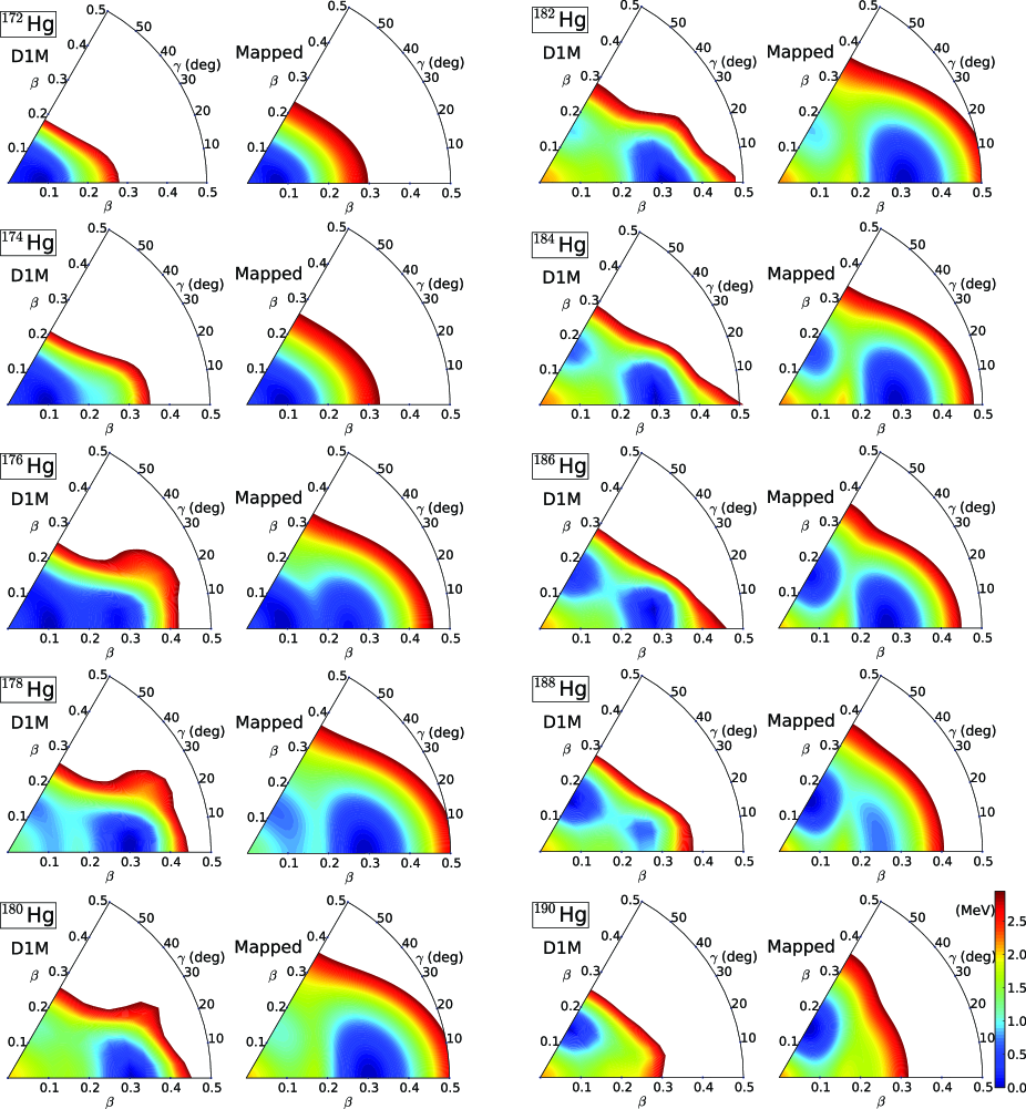
Figure 1: (Color online) Microscopic (“D1M”) and mapped (“Mapped”) potential energy surfaces for the isotopes ^172-190Hg in the ($\beta,\gamma$)-plane are plotted up to 3 MeV from the absolute minimum. The microscopic results are obtained with the Gogny-D1M EDF.

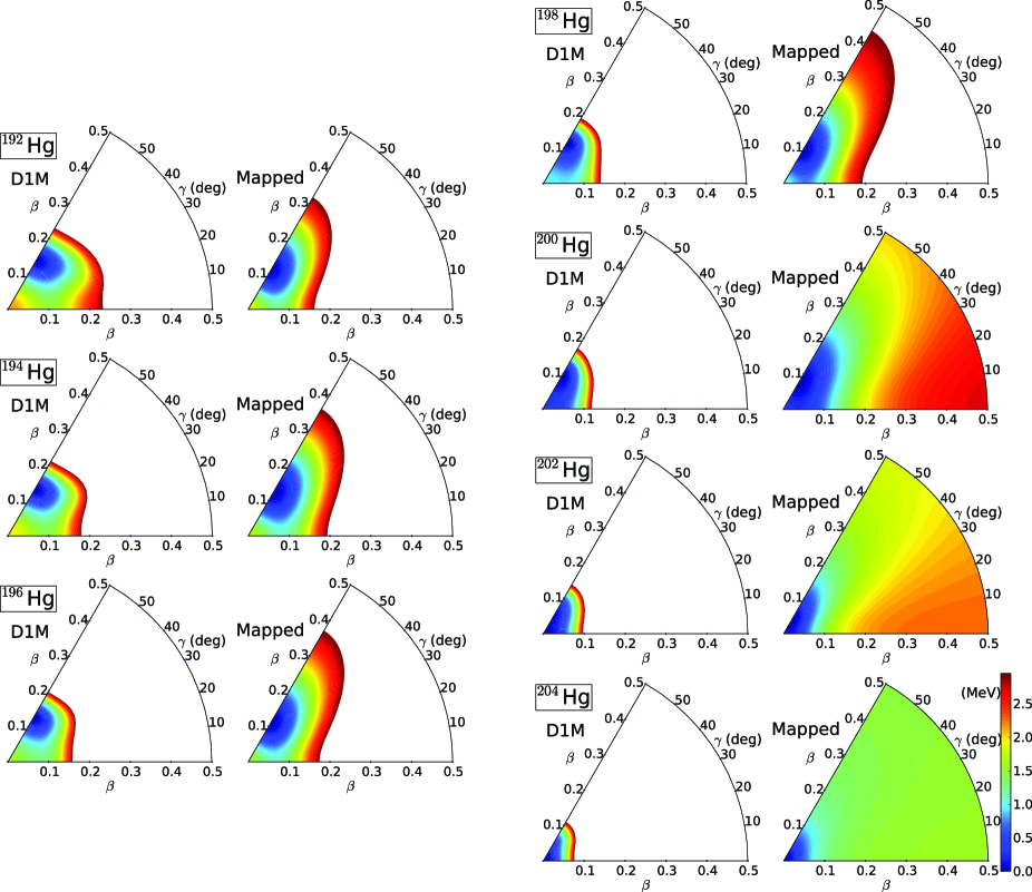
Figure 2: (Color online) Same as Fig. 1, but for ^192-204Hg.

The Gogny-D1M and the mapped energy surfaces of the ^172-204Hg nuclei are plotted in Figs. 1 and 2 in terms of the $q=(\beta,\gamma)$ deformations. We have restricted the plots to configurations up to 3 MeV from the global minimum. Both the microscopic and the mapped energy surfaces give $\beta_{2}$ values consistent with earlier calculations such as the Nilsson-Strutinsky method Nazarewicz (1993) and the collective model approach based on the Gogny-D1S EDF Delaroche et al. (1994), where $\beta_{2}\approx-0.15$ and 0.25-0.3 for the oblate and prolate configurations, respectively. Overall, for each individual nucleus, the topology of the mapped IBM energy surface looks rather similar to the Gogny-D1M one. They both also follow similar systematic changes as a function of the neutron number, as expected.

Starting from ¹⁷²Hg in Fig. 1, one sees a nearly spherical structure with a weakly deformed prolate configuration in both ^172,174Hg. The energy surface suddenly becomes softer along the $\gamma=0^{\circ}$ axis from ¹⁷⁴Hg to ¹⁷⁶Hg. The latter shows two minima with energies within a range of $\approx$ 120 keV. Both minima in ¹⁷⁶Hg are prolate with $\beta\approx 0.1$ and $\beta\approx 0.25$, respectively. On the other hand, the prolate minimum with $\beta\approx 0.3$ becomes more pronounced in ¹⁷⁸Hg while a second one appears in the oblate side with $\beta\approx 0.13$.

The Gogny-D1M energy surfaces for both ^180,182Hg display more developed prolate minima at $\beta\approx 0.3$ while the oblate minimum at $\beta\approx 0.15$ becomes gradually lower in energy when approaching ¹⁸⁴Hg for which the energy surface exhibit a softer $\gamma$-behavior. Within the HFB approximation, the prolate-oblate energy difference in the energy surface reaches a minimum in ¹⁸⁶Hg which signals the most prominent case of shape coexistence in the considered Hg chain. Note that, in ¹⁸⁶Hg, the higher minimum on the prolate side is a bit off the $\gamma=0^{\circ}$ axis, locating at $\gamma\approx 5^{\circ}$. In ¹⁸⁸Hg, one can clearly see that the oblate minimum becomes energetically favoured over the one around $\gamma\approx 10^{\circ}$ on the prolate side. In ¹⁹⁰Hg only the oblate minimum survives.

For the heavier nuclei with $A\geq 192$ in Fig. 2, the prolate minimum diminishes and only the oblate one is seen in ^194-196Hg. This single oblate minimum becomes softer for $A\geq 198$, and approaches $\beta=0$. This implies a structural change from weakly oblate deformed to nearly spherical states. We have also found an almost pure spherical minimum in ²⁰⁴Hg. It should be noted that the corresponding mapped IBM energy surfaces for ^198-204Hg look rather flat when compared with the Gogny-D1M ones. This is a consequence of the limited valance space in these nuclei, close to the shell closure $N=126$, which is not large enough to reproduce the topology of the configurations with energies $\Delta E\geq 1$ MeV. Therefore, we have considered an energy range of up to 1 MeV for the IBM description of the nuclei ^198-204Hg.

The present calculations, based on the Gogny-D1M EDF, predict the oblate minimum to become the dominant one around ^188,190Hg. This is consistent with earlier mean-field calculations based on the D1 Girod and Reinhard (1982) and D1S Delaroche et al. (1994) parametrizations of the Gogny-EDF. Similar results have also been found using the Skyrme-SLy4 EDF Moreno et al. (2006). On the other hand, and at variance with earlier studies with a deformed Woods-Saxson potential Bengtsson and Nazarewicz (1989); Nazarewicz (1993), our calculations predict prolate deformed ground states for some of the considered neutron deficient Hg isotopes. Let us stress that similar results, i.e., prolate ground states, are predicted with the Gogny-D1S parameter set (see compilation of the Gogny-D1S HFB results in CEA ) as well as with other non-relativistic Skyrme Moreno et al. (2006); Bender et al. (2006); Yao et al. (2013) and relativistic NL3 Nikšić et al. (2002) parametrizations. In fact, the so-called NL-SC (Shape Coexistence) parametrization of the relativistic mean-field Lagrangian, which has been specifically adjusted to describe binding energies, radii and deformation in the Lead region, has been introduced in Ref.Nikšić et al. (2002) to account for these problem in the more standard NL3 set. All in all, the most standard relativistic and non-relativistic parametrizations, used to compute nuclear properties all over the nuclear chart, seem to predict prolate ground states at least for some of the neutron deficient Hg isotopes.

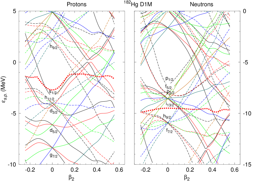
Figure 3: (Color online) The single particle energies obtained by diagonalizing the Hartree- Fock Hamiltonian are plotted as a function of the deformation parameter $\beta_{2}$ for both protons and neutrons and the nucleus ¹⁸²Hg. Full (dashed) lines correspond to positive (negative) parity orbitals. The thick dashed line corresponds to the Fermi level. Also the spherical orbit quantum numbers are given at zero deformation allowing the identification of each orbital by following its evolution from sphericity.

In order to clarify the origin of this result we display in Fig 3 a Nilsson-like plot showing the evolution of the single particle energies of the Hartree-Fock Hamiltonian as a function of the axially symmetric quadrupole deformation parameter $\beta_{2}$ in the nucleus ¹⁸²Hg. The choice of this nucleus is guided by its two minima, one oblate and the other prolate. In the plot, we observe that the deformation of the prolate and oblate minima corresponds to the deformation where the proton $h_{9/2}$ and neutron $i_{13/2}$ orbitals cross the Fermi level. The prolate minimum is to be associated to the crossing of the $K=1/2$ members of the orbitals whereas the oblate minimum to the occupancy of the high-K $K=j$ members.

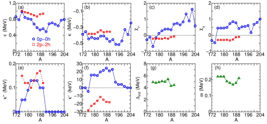
Figure 4: (Color online) Derived IBM parameters (a) $\epsilon_{i}$, (b) $\kappa_{i}$, (c) $\chi_{\nu,i}$, (d) $\chi_{\pi,i}$, (e) $\kappa_{i}^{\prime\prime}$, (f) $\kappa^{\prime}_{i}$, (g) $\Delta_{intr}$ and (h) $\omega$ for the considered ^172-204Hg nuclei as functions of mass number $A$. Note that, in panel (f), the parameter $\kappa^{\prime}_{i}$ is plotted in keV unit. Figure legends in panels (a-f) are indicated in panel (a).

The derived IBM parameters [Eq. (1)] are depicted in Fig. 4 as a function of the mass number $A$. Similarly to its empirical boson number dependence Iachello and Arima (1987); Otsuka et al. (1978b), as well as to our previous findings Nomura et al. (2008, 2010, 2011b), the single $d-$boson energy $\epsilon$ shown in panel a) exhibits a parabolic behavior centered at mid-shell. This also agrees, with the empirical evolution of the $2^{+}$ excited state expected in a given isotope/isotone sequence. The $\epsilon_{1}$ and $\epsilon_{3}$ parameters roughly follow this empirical trend. Contrary to earlier phenomenological fitting calculations within the IBM with configuration mixing Duval and Barrett (1981, 1982), the $d$ boson energy for the intruder configuration $\epsilon_{3}$ is always larger than the one for the normal configuration $\epsilon_{1}$. The interaction strengths $\kappa_{1,3}$, shown in panel b), do not change too much. Nevertheless, they are several times larger than the phenomenological ones ( $\kappa_{1}\approx-0.17\sim-0.14$ MeV and $\kappa_{3}\approx-0.14\sim-0.11$ MeV) Barfield et al. (1983). The reason is that the deformation energy, given by the depth of the minimum in the Gogny-D1M energy surface, turns out to be large compared to what is expected from the $\kappa$ value used phenomenologically.

We observe in Figs. 4(c) and 4(d) that the sum $\chi_{\nu}+\chi_{\pi}$ is positive (negative) for the oblate (prolate) configuration, being consistent with the microscopic energy surface. In many of the phenomenological IBM configuration mixing calculations (e.g., Duval and Barrett (1982)), the $2p$-$2h$ configuration has been considered in the rotational SU(3) limit of the IBM Iachello and Arima (1987) by taking $\chi_{\nu,\pi}=-\sqrt{7}/2\approx-1.3$. The present result does not follow this trend as both the $\chi_{\nu}$ and $\chi_{\pi}$ values for the $2p$-$2h$ configuration are smaller in magnitude than the SU(3) limit of $-\sqrt{7}/2$, reflecting a more pronounced $\gamma$-soft character for the intruder prolate minimum in the Gogny-D1M energy surface.

From Fig. 4(e), one sees that the derived $\kappa^{\prime\prime}_{2}$ value for both ¹⁸⁶Hg and ¹⁸⁸Hg is particularly large in agreement with the Gogny-D1M energy surface [Fig.1] of the two nuclei displaying the most notable $\gamma$ softness on the prolate side in the considered isotopic chain. On the other hand, we assume the $\kappa^{\prime\prime}_{1}$ value, for the single-configuration nuclei ^{172-174,192-204}Hg, to be zero, because neither a triaxial minimum nor notable $\gamma$ softness are observed in the microscopic energy surfaces shown in Figs. 1 and 2.

The $\hat{L}\cdot\hat{L}$ coefficient $\kappa^{\prime}_{i}$, shown in panel f), appears to be stable for the $0p$-$0h$ configuration in ^178-192Hg while a certain decrease in magnitude is observed for the $2p$-$2h$ configuration towards the mid-shell. The sign of $\kappa^{\prime}_{i}$ is of much relevance. In particular, a positive (negative) sign for the normal ($2p$-$2h$) configuration implies that the inclusion of the $\hat{L}\cdot\hat{L}$ term reduces (enlarges) the moment of inertia of the corresponding unperturbed collective band. For the weakly deformed nuclei ^172-176Hg and ^194-204Hg, where only a single configuration is considered, the derived $\kappa^{\prime}_{1}$ value is almost zero or very small in magnitude.

The energy offset $\Delta_{intr}$ in Fig. 4(g) changes with neutron number symmetrically with respect to ¹⁸⁶Hg. The energy needed to excite two protons across the $Z=82$ closed shell becomes maximal for this mid-shell nucleus because the intruder $2p$-$2h$ configuration gains maximal energy through deformation. As can be observed from panel h), the mixing strength $\omega$ decreases with boson number toward the midshell.

IV Results and discussion

In what follows, we compare the results obtained by diagonalizing the mapped IBM-2 Hamiltonian with the available experimental data. Results for spectroscopic observables, including excitation energies, $B$(E2) transition rates and quadrupole moments as well as ground-state properties (mean square charge radii and binding energies) are discussed.

IV.1 Level energy systematics

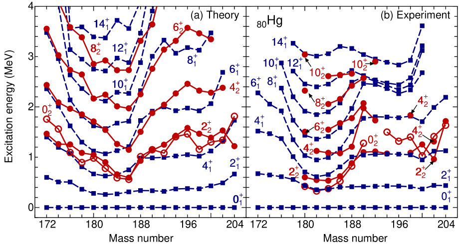
Figure 5: (Color online) Level-energy systematics for ^180-190Hg isotopes with mass number. Theoretical level energies coming from the mapped IBM-2 Hamiltonian based on the Gogny-D1M EDF (a) are compared with the experimental Sandzelius et al. (2009); Julin et al. (2001); Brookhaven National Nuclear Data Center ; Page et al. (2011); Elseviers et al. (2011) (b) energies. The yrast (square) and the non-yrast (circle) states are connected by dashed and solid lines, respectively.

The systematics of the excitation energies in the isotopes ^172-204Hg is shown in Fig. 5. Results are presented for states with excitation energies up to 4 MeV. The theoretical energy levels, obtained through the diagonalization of the mapped IBM-2 Hamiltonian, are compared with the corresponding experimental data Sandzelius et al. (2009); Julin et al. (2001); Brookhaven National Nuclear Data Center ; Page et al. (2011); Elseviers et al. (2011), shown in panel (b). As can be seen in Fig. 5(a), the calculated spectra for ^172,174Hg resemble a vibrational-like behaviour with $R_{4/2}=E(4^{+}_{1})/E(2^{+}_{1})=$2.34 and 2.36, respectively. We also observe close lying $4^{+}_{1}$, $2^{+}_{2}$ and $0^{+}_{2}$ levels, characteristic for the vibrational level structure. Although, the excitation energies for the non-yrast states have not been experimentally measured, the experimental $R_{4/2}$ ratios, i.e., 2.26 (¹⁷²Hg) and 2.27 (¹⁷⁴Hg) deduced from Fig. 5(b), are reproduced well. Going from ¹⁷⁴Hg to ^176,178Hg, the $0^{+}_{2}$ level comes down rapidly in our calculations, being close in energy to the $4^{+}_{1}$ one. This implies that the intruder prolate configuration arises in ¹⁷⁶Hg as a consequence of the IBM-2 configuration mixing. This agrees well with what could be expected from the microscopic energy surface in Fig. 1.

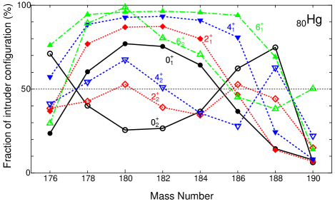
Figure 6: (Color online) Fraction of the intruder $2p$-$2h$ configuration in the wave functions of the $0^{+}_{1,2}$, the $2^{+}_{1,2}$, the $4^{+}_{1,2}$ and the $6^{+}_{1,2}$ excited states of the ^176-190Hg isotopes (in %).

In order to understand the nature of the calculated $0^{+}_{2}$ state for Hg nuclei with $A\geq 176$, we have calculated the probabilities of the different basis states in the wave function of the state of interest. In Fig. 6, we have plotted the fraction of the $2p$-$2h$ component in the wave functions of the $0^{+}_{1,2}$, $2^{+}_{1,2}$, $4^{+}_{1,2}$ and the $6^{+}_{1,2}$ states. The ground-state $0^{+}_{1}$ level for ¹⁷⁶Hg and ¹⁷⁸Hg are predominantly $0p$-$0h$ and $2p$-$2h$, respectively. On the other hand, the opposite behaviour is predicted for the $0^{+}_{2}$ state in each of the two nuclei. Therefore, the present calculation suggests that the bandhead of the intruder configuration becomes energetically favoured at ¹⁷⁸Hg over the lowest $0^{+}$ state of the normal configuration. Note that, from the energy surfaces in Fig. 1, both the $0p$-$0h$ and the $2p$-$2h$ configurations correspond to the prolate deformation in ^176,178Hg.

For the ^180,182Hg nucleus in Fig. 5(a), however, the level energy of the $0^{+}_{2}$ state is much higher than the corresponding experimental data Brookhaven National Nuclear Data Center ; Page et al. (2011); Elseviers et al. (2011). As we will show later, this deviation of the $0^{+}_{2}$ state is mainly due to the fact that the prolate-oblate energy difference is too large in the Gogny-D1M energy surface. Moreover, the present calculation predicts that the ground-state $0^{+}_{1}$ state in the ^180,182Hg nuclei is comprised mainly of the intruder prolate configuration. Precisely, 77.0% (75.4%) of the $0^{+}_{1}$ state of the ¹⁸⁰Hg (¹⁸²Hg) is dominated by the $2p$-$2h$ configuration (see, Fig. 6). However, this contradicts the experimental finding Ulm et al. (1986); Grahn et al. (2009); Elseviers et al. (2011) that the ground-state of these nuclei is weakly deformed oblate configuration. The reason for the contradiction is that, in the microscopic energy surfaces of ^180,182Hg (cf. Fig. 1), the prolate minimum is lower than the oblate one.

In both ^184,186Hg in Fig. 5(a), the excited $0^{+}$ state comes lower in energy, below the $4^{+}_{1}$ energy level. In ¹⁸⁶Hg, in particular, while the $2^{+}_{1}$ level energy is lower than the experimental Brookhaven National Nuclear Data Center value, the $0^{+}_{2}$ excited state is predicted to be the intruder configuration and the oblate bandhead becomes the ground state, as shown in Fig. 6. Also worth noting is that, similarly to ^180,182Hg, the ¹⁸⁴Hg is predicted to have the prolate ground state (see Fig. 6) in contradiction with the data Brookhaven National Nuclear Data Center . From Fig. 6, we notice that the two configurations are strongly mixed for each of the low-lying states of ^184,186Hg. This strong mixing and the subsequent level repulsion may partly account for the kink observed in the calculated yrast states with $J^{\pi}\geq 10^{+}$ at ¹⁸⁴Hg in Fig. 5(a).

In accordance with the evolution of deformation in each configuration, in Fig. 5(a) the yrast and the non-yrast states other than $0^{+}_{2}$ states keep lowering toward the mid-shell $N=104$, while these levels are generally higher than the experimental ones in Fig. 5(b).

Most of the levels in Fig. 5(a) increase their energies when going from the near mid-shell nuclei ^184,186Hg to ¹⁸⁸Hg, a behaviour that is consistent with the experimental data in Fig. 5(b). This sudden change in the energy level is also consistent with the Gogny EDF mean-field energy surface in Fig. 1, where we observe that the intruder prolate minimum becomes less significant in ¹⁸⁸Hg than in ¹⁸⁶Hg. In the ground state of ¹⁸⁸Hg, the oblate normal configuration becomes much more populated than the intruder prolate configuration in Fig. 6.

From Fig. 6, one sees that only a small fraction of the intruder component plays a role in the low-lying states of ¹⁹⁰Hg. The excited $0^{+}$ state is originated almost purely from a single oblate configuration, consistently with the empirical observation Delaroche et al. (1994).

Back to Fig. 5, from ¹⁹⁰Hg to heavier isotopes, the calculated energy levels of yrast states are almost constant as a function of mass number in agreement with the experimental trend. The energy of most of the non-yrast states keep increasing as the $N=126$ shell closure is approached. In the present model, only the single oblate configuration is required to describe those nuclei with $192\leq A\leq 204$. A comparison between the experimental and theoretical level structures for ^192-200Hg in Figs.5(a) and 5(b) reveals that, while the signatures of a vibrational-like level distribution ($R_{4/2}$ ratio and similar $4^{+}_{1}$, $2^{+}_{2}$, and $0^{+}_{2}$ energies) suggested experimentally is roughly reproduced, the calculations suggest a slightly more deformed rotational character than the experiment. This means that the predicted ground-state band is more compressed for the $2^{+}_{1}$ state but more stretched for $J^{\pi}\geq 6^{+}$ levels than in the experiment. In particular, the theoretical $R_{4/2}$ ratio is generally $R_{4/2}\approx 2.7\sim 2.8$, while experimental values are $R_{4/2}\approx 2.5\sim 2.6$.

The nuclei ^200-204Hg show deep spherical minima in their energy surfaces as seen in Fig. 2. As a consequence, the theoretical $2^{+}_{1}$, $4^{+}_{1}$ and $0^{+}_{2}$ level energies rapidly increase when the $N=126$ shell closure is approached. The excitation energies are much larger than the experimental values as a consequence of the IBM model space that excludes pure spherical configurations.

To summarize the results in Fig. 5(a), we have shown that the present method describes the shape transition from the near spherical or weakly deformed structures to the manifest shape coexistence near the mid-shell nucleus ¹⁸⁴Hg, and to the weakly oblate deformed shapes and the vibrational structure near the $N=126$ shell closure. Although the empirical evidence that the lowest two $0^{+}$ states of the nuclei around ¹⁸⁴Hg are originated either from the $0p$-$0h$ or the $2p$-$2h$ configurations is reproduced, a major deviation from experiment and from earlier phenomenological studies arises in the inverted level structure in ^180,182,184Hg and the too compressed $2^{+}_{1}$ level energies overall. In the next section, Sec. IV.2, we address these problems in more detail.

IV.2 Shape coexistence

Of all the Hg isotopes, the nuclei ^{182,184,186,188}Hg near the neutron mid-shell $N\approx 104$ are the ones exhibiting the most clear signatures of coexistence of different shapes. In order to identify the different components the level scheme, including both the in-band and the inter-band E2 transition rates is analyzed. To facilitate the comparison with the experimental data, the excited states shown below will be classified as either oblate or prolate bands based on the prolate-oblate predominance of the wave function of the state, shown in Fig. 6, or alternatively on the E2 transition sequence.

The $B({\rm E2};J\rightarrow J^{\prime})$ transition rate reads

$$B({\rm E2};J\rightarrow J^{\prime})=\frac{1}{2J+1}|\langle J^{\prime}||\hat{T}^{({\rm E2})}||J\rangle|^{2},$$ (10)

where $|J\rangle$ ($|J^{\prime}\rangle$) represents the wave function of the initial (final) state with spin $J$ ($J^{\prime}$). The E2 operator $\hat{T}^{\rm(E2)}$ is given as $\hat{T}^{\rm(E2)}=\sum_{\rho,i=1,3}{\cal\hat{P}}_{i}e_{\rho,i}\hat{Q}_{\rho}^{\chi_{\rho,i}}{\cal\hat{P}}_{i}$, where $\hat{Q}_{\rho}^{\chi_{\rho,i}}$ is identified with the quadrupole operator in Eq. (2). We consider the same $\chi_{\rho,i}$ value as the one used in the diagonalization of the Hamiltonian in Eq. (1). This is equivalent to the so-called consistent-Q formalism in the IBM-1 Warner and Casten (1983). The boson effective charge $e_{\rho,i}$ is assumed to be the same for protons and neutrons, i.e., $e_{\nu,i}=e_{\pi,i}\equiv e_{i}$. In order to obtain an overall systematic agreement with the typical experimental $B({\textnormal{E2}};2^{+}_{1}\rightarrow 0^{+}_{1})$ value of $\approx 40-60$ Weisskopf units (W.u.), we adopt the values $e_{1}=e_{3}=0.11$ $e$b for ^182,184Hg, $e_{1}=0.07$ $e$b and $e_{3}=0.15$ $e$b for ¹⁸⁶Hg, $e_{1}=0.15$ $e$b and $e_{3}=0.07$ $e$b for ^{176,178,180,188,190}Hg, and $e_{1}=0.15$ $e$b for all other nuclei described only with a single configuration.

IV.2.1 ¹⁸²Hg

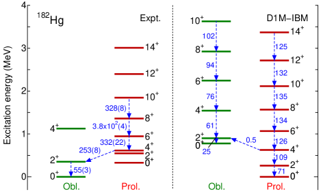
Figure 7: (Color online) Detailed level scheme for the ¹⁸²Hg nucleus. The level energies and the $B$(E2) values in Weisskopf units (numbers written along arrows) obtained from the mapped IBM-2 Hamiltonian based on the Gogny-D1M EDF are shown. The oblate and the prolate bands are indicated by “Obl.” and “Prol.”, respectively. The experimental data are taken from Ref. Brookhaven National Nuclear Data Center .

The detailed level scheme of the nucleus ¹⁸²Hg is shown in Fig. 7. The spectra and the $B$(E2) transition strengths, computed from the mapped IBM-2 Hamiltonian based on the Gogny-D1M EDF, are compared with the relevant experimental Brookhaven National Nuclear Data Center level scheme in the same figure.

The calculation predicts the ground-state band to have an intruder prolate nature, whereas experimentally the ground state of ¹⁸²Hg has been suggested to be of oblate nature Ulm et al. (1986). A clear collective pattern is seen from the calculated E2 transition sequence for both the predicted prolate and oblate bands, while the experimental $10^{+}\rightarrow 8^{+}$, $8^{+}\rightarrow 6^{+}$ and $6^{+}\rightarrow 4^{+}$ E2 transition rates in the prolate band are underestimated in the present calculation. Major deviation from the experimental data occurs in the inter-band transition from the $4^{+}$ state in the prolate band to the $2^{+}$ state in the oblate band. The corresponding experimental value, $B({\rm E2};4^{+}_{1}\rightarrow 2^{+}_{1})=253(8)$ W.u, is quite large in comparison to the $2^{+}_{1}\rightarrow 0^{+}_{1}$ E2 transition strength reflecting the very strong mixing between the different configurations. In our calculations, however, relative to the $B({\rm E2};2^{+}_{1}\rightarrow 0^{+}_{1})=71$ W.u., the inter-band transition $B({\rm E2};4^{+}_{1}\rightarrow 2^{+}_{2})=0.5$ W.u. appears to be too small, implying that the mixing effect is not significant. This could be relevant for the predicted level structure where, in comparison to the experimental data, the energy levels of the second band (which is of oblate nature in the present work) are systematically higher than those of the ground-state band, giving rise to a weak E2 transition. This problem is traced back to the unexpectedly large energy difference between the prolate and the oblate HFB minima (see, Fig. 1).

A similar argument holds for ¹⁸⁰Hg, where the contents of the two configurations in the wave functions of the low-lying states look similar to the ones of ¹⁸²Hg (see Fig. 6).

IV.2.2 ¹⁸⁴Hg

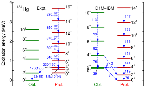
Figure 8: (Color online) Same as Fig. 7, but for ¹⁸⁴Hg. The experimental data are taken from Ref. Brookhaven National Nuclear Data Center .

The results for the ¹⁸⁴Hg nucleus shown in Fig. 8 look rather similar to the ones obtained for ¹⁸²Hg depicted in Fig. 7. Both show a prolate ground state and the $B$(E2) systematics in each band looks similar. In particular, the weak inter-band $B$(E2) transitions between the $4^{+}_{1}$ and the $2^{+}_{2}$ excited states as well as between $4^{+}_{2}$ and the $2^{+}_{1}$ states indicate that the mixing between the two configurations may not have a significant effect. The reason for this discrepancy seems to be the same as in ¹⁸²Hg.

IV.2.3 ¹⁸⁶Hg

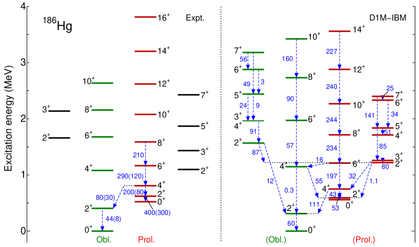
Figure 9: (Color online) Same as Fig. 7, but for ¹⁸⁶Hg nucleus. The experimental data are taken from Ref. Brookhaven National Nuclear Data Center . To help identify the energies of $3^{+}_{2}$ and $4^{+}_{4}$ states, closely lying to with other, $E(3^{+}_{2})=1.970$, $E(4^{+}_{4})=1.959$ (in MeV), and the relevant $B$(E2) transitions are $B({\rm E2};3^{+}_{2}\rightarrow 2^{+}_{4})=91$, $B({\rm E2};5^{+}_{2}\rightarrow 3^{+}_{2})=9$, $B({\rm E2};5^{+}_{2}\rightarrow 4^{+}_{4})=24$ (in W.u.) in the right panel.

The empirical prolate-oblate assignment of the lowest two collective bands in ¹⁸⁶Hg suggests Ma et al. (1993) that the band built on the $0^{+}_{1}$ state is of oblate nature while the one on the $0^{+}_{2}$ state is of prolate. Following this assignment, the $0^{+}$ ground-state in ¹⁸⁶Hg (see, Fig. 9) is predicted to be of oblate nature in the present work. The $0p$-$0h$ and the intruder $2p$-$2h$ configurations are substantially mixed in the wave functions of the lowest two $0^{+}$ states. According to the results of Fig. 6, the $0^{+}_{1}$ ($0^{+}_{2}$) state contains 36.7 (62.3)% of the intruder $2p$-$2h$ configuration. In fact, the prolate configuration is quite notable in the mean-field energy surface shown in Fig. 1. Our calculations seem to follow the experimental energy levels with up to $J^{\pi}=4^{+}$ in the oblate band, the energy levels in the intruder prolate band, and some of the available $B$(E2) data. The deviation is seen in the stretching of the $J^{\pi}=6^{+}_{2}$ and the $8^{+}_{2}$ energy levels in the oblate band, and in the $B({\textnormal{E2}};4^{+}_{1}\rightarrow 2^{+}_{2})$ and $B({\textnormal{E2}};2^{+}_{2}\rightarrow 0^{+}_{2})$ in the prolate band. In addition, rather irregular in-band $B$(E2) transitions are found in the $4^{+}\rightarrow 2^{+}$ transitions, which are indeed quite weak compared to the inter-band $4^{+}\rightarrow 2^{+}$ transitions. This implies a pronounced mixing between the two configurations.

We also analyze the structure of higher-lying bands, including odd-spin states as there are sufficient experimental data to compare with. From Fig. 9 one sees that the present calculation also reproduces the excitation energies of odd-spin states rather well. The odd-spin states, $3^{+}_{1}$, $5^{+}_{1}$ and $7^{+}_{1}$ ($3^{+}_{2}$, $5^{+}_{2}$ and $7^{+}_{2}$), are predicted to be the members of the prolate (oblate) band. Due to the strong E2 transition sequence, it is also likely that a set of the states $2^{+}_{3}$, $3^{+}_{1}$, $4^{+}_{3}$, $5^{+}_{1}$, $6^{+}_{3}$ and $7^{+}_{1}$ ($2^{+}_{4}$, $3^{+}_{2}$, $4^{+}_{4}$, $5^{+}_{2}$, $6^{+}_{4}$ and $7^{+}_{2}$), forms a quasi-$\gamma$, i.e., $K^{\pi}=2^{+}$, band for the prolate (oblate) configuration. These two quasi-$\gamma$ bands seem to be close in energy, with $2^{+}$ bandheads being within 400 keV. One can also observe in both quasi-$\gamma$ bands quite strong E2 transitions from the $3^{+}$ level to the corresponding $2^{+}$ bandhead, which is in the same order of magnitude as the $2^{+}\rightarrow 0^{+}$ E2 transition in each $K^{\pi}=0^{+}$ band, and those between the members of the quasi-$\gamma$ band. Note that this prediction (i.e., the existence of the two quasi-$\gamma$ bands) is consistent with the empirical assignment of these levels Delaroche et al. (1994), including the collective model description based on Gogny-D1S EDF. In addition, one should notice that the quasi-$\gamma$ band in the prolate configuration looks similar to the one predicted within the rigid-triaxial rotor model of Davydov and Filippov, characterized by the the doublets ($2^{+}_{\gamma}$,$3^{+}_{\gamma}$), ($4^{+}_{\gamma}$,$5^{+}_{\gamma}$), ($6^{+}_{\gamma}$,$7^{+}_{\gamma}$), …etc Davydov and Filippov (1958). Empirically the Davydov-Filippov picture is rarely realized. Therefore, the level structure in the proposed quasi-$\gamma$ band of prolate nature (in Fig. 9) seems to be just a consequence of the mixing, which pushes up the energy levels of the even-spin states in the band.

From the comparison with the IBM phenomenology for ¹⁸⁶Hg Barfield et al. (1983), we notice that the present result exhibits a similar level of agreement with the experiment regarding the energy spectra of the oblate ground-state band with $J\leq 6^{+}$. Our result reproduces slightly better the $3^{+}_{1}$ state while, as discussed in Sec. IV.1, the prolate $0^{+}_{2}$ band-head energy is a bit more overestimated.

That the oblate band is the ground state and that the intruder prolate band is built on the $0^{+}_{2}$ state, are consistent with the result of the most recent projected GCM calculation of the ¹⁸⁶Hg nucleus with the Skyrme SLy6 functional Chabanat et al. (1998) (see Fig. 16 in Yao et al. (2013)). However, there is a certain quantitative difference between the two descriptions.

IV.2.4 ¹⁸⁸Hg

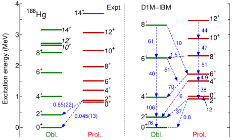
Figure 10: (Color online) Same as Fig. 7, but for ¹⁸⁸Hg nucleus. The experimental data are taken from Ref. Brookhaven National Nuclear Data Center .

For the ¹⁸⁸Hg nucleus, the results shown in Fig. 10 show a rather reasonable agreement between theory and experiment regarding the band structure and including the energy level of the $0^{+}_{2}$ state. Note that the experimental $10^{+}_{1}$, $12^{+}_{1}$ and $14^{+}$ states, written in italic in Fig. 10, are assigned to be members of a oblate band different from the ground-state oblate band Brookhaven National Nuclear Data Center . A pronounced mixing between the two configurations is confirmed from the $B$(E2) values of the $6^{+}_{1,2}\rightarrow 4^{+}_{1,2}$ transitions. They reflect the sizable amount of mixing seen in the wave functions of the two $6^{+}$ excited states in Fig. 6 [the wave function of the $6^{+}_{1}$ ($6^{+}_{2}$) state contains 69.1 (38.2)% of the $2p$-$2h$ component]. While the dominance of the $2^{+}_{2}\rightarrow 2^{+}_{1}$ E2 transition over the $2^{+}_{2}\rightarrow 0^{+}_{1}$ transition roughly follows the experimental trend, their absolute values are much larger than the data. The reason is again the very strong mixing between the low-spin states. In ¹⁸⁸Hg, any sequence of the quasi-$\gamma$ band structure has not been obtained in our calculations. On the other hand, the predicted $3^{+}_{1}$ energy (1.437 MeV) agrees well with the data (1.455 MeV) Brookhaven National Nuclear Data Center .

IV.2.5 Mixing matrix element

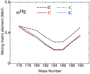
Figure 11: (Color online) Matrix element of the mixing interaction $|\langle\hat{H}_{mix}\rangle|$ between the $0^{+}_{1}$, $2^{+}_{1}$, $4^{+}_{1}$ and the $6^{+}_{1}$ excited states diagonalized in the unperturbed $0p$-$0h$ configuration space and the corresponding states resulting from the diagonalization in the unperturbed $2p$-$2h$ configuration space for the nuclei for which configuration mixing calculation is performed.

In the last two sections we have found that, in the ^186,188Hg nuclei, the mixing between the two configurations can be too large for the low-spin states, resulting in some discrepancies with the experimental data. To shed some light into the origin of the mixing we display in Fig. 11 the matrix element of the mixing interaction $\langle\hat{H}_{mix}\rangle$, that couples the $0^{+}_{1}$, $2^{+}_{1}$, $4^{+}_{1}$ and $6^{+}_{1}$ excited states resulting from the unperturbed $0p$-$0h$ and $2p$-$2h$ Hamiltonians for ^176-190Hg.

These results for the mixing matrix elements may explain the calculated level energy spacings, e.g., between $2^{+}_{1}$ and $2^{+}_{2}$ states in ¹⁸⁶Hg which is larger than the corresponding experimental data, and also confirm the too strong mixing in these low-spin states. To compare with the schematic two-level mixing calculations, the present $|\langle\hat{H}_{mix}\rangle_{0^{+}_{1}}|$ value of 281 keV for ¹⁸⁶Hg is of the same order of magnitude as the earlier result of $>110$ keV JOSHI et al. (1994), but is much larger than a more recent result of $69^{+25}_{-41}$ keV Scheck et al. (2010).

For the ¹⁸⁸Hg nucleus, the mixing matrix element $|\langle\hat{H}_{mix}\rangle|\approx 280$ keV for the unperturbed $2^{+}_{1}$ and $6^{+}_{1}$ states (cf. Fig. 11) could explain the quenching of the $2^{+}$ level and the stretching of $J^{\pi}\geq 6^{+}$ level in the ground-state band, as shown in Fig. 10. On the other hand, the mixing matrix element for the unperturbed $0^{+}_{1}$ state for ¹⁸⁸Hg is 371 keV, which seems to be large enough to account for the calculated $0^{+}_{2}$ excitation energy of 1012 keV.

IV.2.6 Discussion

To summarize the results of Sec. IV.2, we list the main deficiencies of our model in its current version: (i) In ¹⁸²Hg (as well as ¹⁸⁴Hg), the predicted band structure is in contradiction with the empirical assignment, i.e., the ground-state band is of weakly deformed oblate nature. (ii) In ^184,186,188Hg, irregular patterns appeared in some of the energy levels in the oblate band and in the $B$(E2) transitions between low-spin states. Overall, the $2^{+}_{1}$ energy level has been predicted to have an energy too low in comparison with the experimental data.

A major reason for the inversion of the prolate and the oblate bands in ^180,182,184Hg could be the peculiar topology of the microscopic energy surface, i.e., the energy difference between the prolate and oblate mean-field minima. This seems to be quite likely since, as we have shown in the Gogny-D1M energy surfaces e.g., for ¹⁸⁰Hg (¹⁸²Hg) in Fig. 1, the oblate minimum at $\beta\approx 0.15$ looks higher in energy approximately by 1.1 (0.9) MeV than intruder prolate minimum at $\beta\approx 0.3$. This prolate-oblate energy difference is too large to reproduce the energy spacing of the experimental $0^{+}_{1}$ and $0^{+}_{2}$ levels of $\approx 400$ keV in ^180,182Hg, and to explain the empirical systematics, i.e., the weakly oblate deformed ground-state band. On the other hand, as pointed out in Sec. III, most of the standard EDF parameterizations, used for the global description of the nuclear properties over the whole periodic table, commonly predict the prolate ground state in the mean-field energy surface. We note that, in the recent beyond mean-field calculation on the low-lying structure in the neutron deficient Hg isotopes Yao et al. (2013), the prolate ground state has been predicted in the ^180,182,184Hg nuclei, similarly to our results.

Another reason can be that the IBM-2 parameters deduced with our method are not good enough to describe all the details of the experimental low-lying states. For instance, the too strong mixing in the low-spin states in ^186,188Hg can be traced back to the value for the mixing strength $\omega$ used in this work that perhaps is so large as to make the energy spacing between $0^{+}_{1}$ and $0^{+}_{2}$ states larger than experimental data. The discrepancies in the $B$(E2) systematics, as well as the stretching of the lower band, may arise from the fact that the derived quadrupole-quadrupole interaction $\kappa_{i}$ is rather large, being more than twice as large as the one used in the earlier IBM-2 phenomenology Duval and Barrett (1981, 1982); Barfield et al. (1983). Such large value of $|\kappa_{i}|$ reflects that the deformation energy, measured by the depth of the minimum, in the Gogny-D1M is unexpectedly large. This seems to be a common feature for any EDF parametrization, and is consistent with the conclusions in our previous studies in other isotopic chains (e.g., Nomura et al. (2010, 2011b)). In the case where only a single minimum is concerned, the effect of the too strong quadrupole-quadrupole interaction could be effectively included in the boson effective charge, leading to a reasonable agreement with the experiment Nomura et al. (2012b). However, this is not the case with the present work because we consider much more complex systems with more then one configurations and also there are so many Hamiltonian parameters and (four) adjustable effective charges. Therefore, it is quite unlikely that a significantly better agreement with the experimental $B$(E2) systematics could be obtained only by adjusting the effective charges.

IV.3 Spectroscopic quadrupole moment

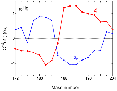
Figure 12: (Color online) Calculated spectroscopic quadrupole moments $Q^{(s)}$ for the lowest two excited $2^{+}$ states of the considered Hg nuclei as functions of mass number.

To confirm from an alternative perspective whether each individual Hg nucleus is oblate or prolate deformed we have also analyzed the spectroscopic quadrupole moments for the lowest two $2^{+}$ excited states, which belong either to the first oblate or prolate band for the near mid-shell nuclei. The spectroscopic quadrupole moment $Q^{(s)}$ for a state with spin $J$ reads

$$Q^{(s)}(J)=\sqrt{\frac{16\pi}{5}}\left(\begin{array}[]{ccc}J&2&J\\ -J&0&J\\ \end{array}\right)\langle J||\hat{T}^{({\rm E2})}||J\rangle.$$ (13)

The overall systematic trend in $Q^{(s)}(2^{+}_{1,2})$ seems to correlate well with the evolution of mean-field minima shown in Figs. 1 and 2 and with the structure of the corresponding wave functions in Fig. 6.

The calculated quadrupole moments for the $2^{+}_{1}$ and the $2^{+}_{2}$ states in all the considered nuclei ^172-204Hg, are shown in Fig. 12. For the lightest isotopes ^172,174Hg, considered in a single configuration, $Q^{(s)}(2^{+}_{1})<0$ confirms the prolate deformation in the ground state. At the ¹⁷⁶Hg nucleus, where the two prolate configurations are considered, both $Q^{(s)}(2^{+}_{1})$ and $Q^{(s)}(2^{+}_{2})$ are negative, as expected. From ¹⁷⁸Hg to ¹⁸⁴Hg, $Q^{(s)}(2^{+}_{1})<0$ ($Q^{(s)}(2^{+}_{2})>0$) gradually increases in magnitude, consistently with the growing prolate (oblate) minimum in the ground state. For ¹⁸⁶Hg, $Q^{(s)}(2^{+}_{2})$ changes its sign as the $2^{+}_{2}$ belongs to the prolate band, while the negative value of $Q^{(s)}(2^{+}_{1})$ contradicts the corresponding energy surface in Fig. 1 and the level scheme in Fig. 9, where the ground state is oblate deformed. Nevertheless, the magnitude of $Q^{(s)}(2^{+}_{1})<0$ for the ¹⁸⁶Hg nucleus is quite small, due to the significant effects of the configuration mixing in the $2^{+}_{1}$ state (Fig. 6) and the triaxiality (Fig. 1), as compared to other isotopes. From ¹⁸⁸Hg to the heavier isotopes, the predicted $Q^{(s)}$ systematics is in agreement with the energy surfaces in Figs. 1 and 2, with $Q^{(s)}(2^{+}_{1})>0$ and $Q^{(s)}(2^{+}_{2})<0$), indicating the oblate ground-state band, both decreasing in magnitude as approaching the neutron shell closure $N=126$.

IV.4 Transition quadrupole moment

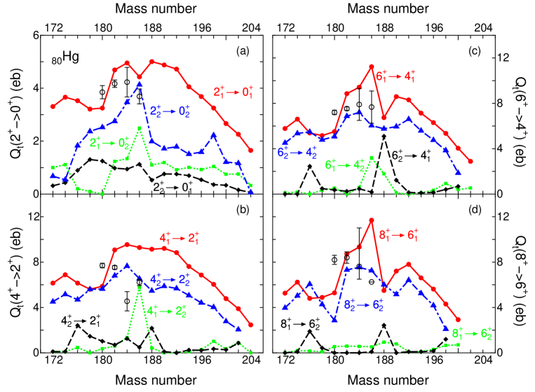
Figure 13: (Color online) The calculated transition quadrupole moment $Q_{t}(J\rightarrow J-2)$ for $J^{\pi}=2^{+}$ (a), $4^{+}$ (b), $6^{+}$ (c) and $8^{+}$ (d) states compared with the experimental $Q_{t}$ values for transitions between the yrast states Grahn et al. (2009); Proetel et al. (1974); Ma et al. (1986) (open circles).

From the $B({\textnormal{E2}};J\rightarrow J^{\prime})$ transition rates, one can extract the transition quadrupole moment $Q_{t}(J\rightarrow J^{\prime})$ for which there are a number of available experimental data to compare with. $Q_{t}(J\rightarrow J^{\prime})$ is related to the $B({\textnormal{E2}};J\rightarrow J^{\prime})$ value through

$$B({\textnormal{E2}};J\rightarrow J^{\prime})=\frac{5}{16\pi}(J200|J^{\prime}0)^{2}\{Q_{t}(J\rightarrow J^{\prime})\}^{2}$$ (14)

Figure 13 exhibits the calculated $Q_{t}(J\rightarrow J-2)$ value for $J^{\pi}=2^{+}$ (a), $4^{+}$ (b), $6^{+}$ (c) and $8^{+}$ (d) states compared with the experimental $Q_{t}$ values for the transition between the yrast states Proetel et al. (1974); Ma et al. (1986); Grahn et al. (2009). In each panel, the transitions between the yrast $J^{+}$ and $(J-2)^{+}$ states and between the non-yrast ones are strong in most of the nuclei. In the nuclei around the mid-shell nucleus ¹⁸⁴Hg, the transition between the yrast states correspond to the in-band E2 transitions within $0p$-$0h$ or $2p$-$2h$ band with strong collectivity and are particularly large in Fig. 13. One of the $Q_{t}$ values for the two in-band transitions follows the experimental data. On the other hand, the transitions between the yrast $J^{+}$ and the non-yrast $(J-2)^{+}$, or vice versa, are overall weak other than the ¹⁸⁶Hg nucleus in Figs. 13(a), 13(b) and 13(c), and the ¹⁸⁸Hg in Figs. 13(c) and 13(d), where the mixing between the two configurations turned out to be significant in the present calculation.

One can also deduce the deformation parameter $\beta_{t}(J\rightarrow J-2)$ from $Q_{t}$ through the relation

$$\beta_{t}(J\rightarrow J-2)=\frac{\sqrt{5\pi}}{3ZR^{2}}Q_{t}(J\rightarrow J-2),$$ (15)

where $R=1.2A^{1/3}$ fm. As examples, the calculated values $\beta_{t}(2^{+}_{1}\rightarrow 0^{+}_{1})\approx 0.15-0.17$ of ^184,186,188Hg, corresponding to the oblate configuration, is consistent with the experimental values $\beta_{t}(2^{+}_{1}\rightarrow 0^{+}_{1})=0.15(2)$ for ¹⁸⁴Hg Ma et al. (1986) and $0.13(1)$ for ¹⁸⁶Hg Proetel et al. (1974), and as well as with the minimum at $\beta\approx 0.15$ in the mean-field energy surfaces in Fig. 1. However, the present $\beta_{t}(2^{+}_{2}\rightarrow 0^{+}_{2})$ value for the ¹⁸⁶Hg (¹⁸⁸Hg) nucleus, corresponding to the prolate deformation, is too small, $\beta_{t}(2^{+}_{2}\rightarrow 0^{+}_{2})\approx 0.15$ (0.17) than the prolate mean-field minimum at $\beta\approx 0.3$ (cf. Fig. 1). The reason are the too strong mixing in these nuclei and also the $\gamma$-softness in the prolate configuration. For ¹⁸²Hg (¹⁸⁰Hg), where the prolate band is predicted to be the lowest band (cf. Fig. 7), $\beta_{t}(2^{+}_{1}\rightarrow 0^{+}_{1})=0.12$ (0.12), which is again too small compared to the prolate mean-field minimum at $\beta\approx 0.3$, whereas the present $\beta_{t}(2^{+}_{2}\rightarrow 0^{+}_{2})=0.12$ (0.09) for oblate configuration agrees with the oblate mean-field minimum at $\beta\approx 0.15$.

IV.5 Ground-state properties

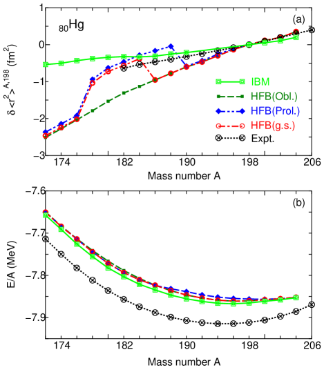
Figure 14: (Color online) The mean square charge radii $\delta\langle r^{2}\rangle^{A,198}$ (a) and the ground-state energy per nucleon $E/A$ (b) for the considered ^172-204Hg. In each panel, the HFB results corresponding to the oblate and the prolate minima, as well as the global minima (one of the former two), and the IBM mixing results for the $0^{+}_{1}$ state are shown. The experimental data have been taken from Angeli (2004) and WWW Table of Atomic Masses for $\delta\langle r^{2}\rangle^{A,198}$ and $E/A$, respectively.

It is worthwhile to compare the ground-state properties of the considered Hg nuclei obtained with the mean field calculation, with the wealth of the available experimental data. In this section we analyze the mean square charge radii and the binding energies. The former plays a relevant role as an indicator of the character of the ground state deformation.

In the HFB method, the charge radius is obtained as the mean value of the $r^{2}$ operator for each of the oblate and prolate minima. In the configuration mixing IBM-2 framework, the charge radius $\langle r^{2}\rangle$ is connected to the matrix element of the E0 operator. The E0 operator $\hat{T}^{\textnormal{(E0)}}$ is given as Iachello and Arima (1987)

$$\hat{T}^{\textnormal{(E0)}}=\sum_{i=1,3}\sum_{\rho=\nu,\pi}\hat{\cal P}_{i}(\beta_{i,\rho}\hat{n}_{d\rho,i}+\gamma_{i,\rho}N_{\rho,i})\hat{\cal P}_{i},$$ (16)

with four parameters $\beta_{i,\rho}$ and $\gamma_{i,\rho}$. The mean square radius $\langle r^{2}\rangle$ is written as

$$\langle r^{2}\rangle=\langle r^{2}_{c}\rangle+\langle\hat{T}^{\textnormal{(E0)}}\rangle_{0^{+}_{1}}.$$ (17)

$\langle r^{2}_{c}\rangle$ represents the contribution from the inert core, which is omitted here since we discuss the $\langle r^{2}\rangle$ values relative to a particular nucleus. For the parameters in the E0 operator of the IBM-2, we adapt the values used in the study of the isomer shift in ^184-200Hg Barfield et al. (1983), $\beta_{1,\nu}=\beta_{3,\nu}=-0.068$ fm², $\beta_{1,\pi}=\beta_{3,\pi}=0$ fm², $\gamma_{1,\nu}+\gamma_{3,\nu}=-0.083$ fm² and $\gamma_{1,\pi}=\gamma_{3,\pi}=0$ fm². For $\gamma_{1,\nu}$ and $\gamma_{3,\nu}$, the average $\gamma_{1,\nu}=\gamma_{3,\nu}=-0.0415$ fm² is taken. Also, to make the radius in the IBM-2 change linearly when crossing the mid-shell, we approximately correct the boson number $N_{\nu,i}$ in Eq. (16) so that $N_{\nu}$ runs from 2 (²⁰⁴Hg) to 17 (¹⁷²Hg) and should be replaced with $N_{\nu}^{\prime}=(126-2N_{\nu})/2$.

In Fig. 14(a) we compare the mean square charge radii relative to the ¹⁹⁸Hg nucleus, $\delta\langle r^{2}\rangle^{A,198}=\langle r^{2}\rangle^{A}-\langle r^{2}\rangle^{198}$, calculated within the HFB and the IBM-2, with the experimental data taken from Angeli (2004). The HFB results for both the oblate and prolate minima have similar values for $A=174-176$ and $A=190-204$ and change linearly with mass. But around the near mid-shell nucleus ¹⁸⁴Hg, the HFB charge radius computed with the prolate minimum wave function becomes significantly larger than the one for the oblate minimum, being in a better agreement with the data for these nuclei exhibiting the prolate intruder configuration. The reason for this behaviour is the large quadrupole deformation for the minima in these nuclei. In this region, shape mixing would lead to a ground state charge radius in between the prolate and oblate results. Both the HFB radii obtained at the prolate and oblate minima have a linear behaviour with mass number similar to the experimental data. For the IBM-2 result, on the other hand, one should also notice the linear change with $A$, which furthermore turns out to be quite consistent with the data for ^182-204Hg, apart from a potential ambiguity in a particular choice of the E0 parameters. A future experiment should clarify how the $\delta\langle r^{2}\rangle$ systematics is extrapolated to $A\leq 180$.

Using the E0 operator in Eq. (16), we also calculate the $\rho^{2}_{\textnormal{E0}}$ value between $0^{+}_{1}$ and $0^{+}_{2}$ states. $\rho_{\textnormal{E0}}(0^{+}_{2}\rightarrow 0^{+}_{1})$ is written as

$$\rho_{\textnormal{E0}}(0^{+}_{2}\rightarrow 0^{+}_{1})=\frac{Z}{R^{2}}\langle 0^{+}_{1}|\hat{T}^{\textnormal{(E0)}}|0^{+}_{2}\rangle$$ (18)

To compare with a few available data for ¹⁸⁴Hg (¹⁸⁸Hg) nucleus, the calculated and the experimental Kibédi and Spear (2005) $\rho^{2}_{\textnormal{E0}}(0^{+}_{2}\rightarrow 0^{+}_{1})\times 10^{3}$ values are 4.670 (1.447) and 3.2$\pm$1.1 (7$\pm$3), respectively, which are in the same order of magnitude.

It is also possible, in the present framework, to compare the calculated binding energy with the experiment. Figure 14(b) displays the comparison between theoretical and the experimental WWW Table of Atomic Masses ground-state energy per nucleon $E/A$. The HFB results are based on the mean-field ground-state energies for oblate and prolate minima. In the IBM-2, on the other hand, the ground-state energy is obtained by including the global term in the Hamiltonian Eq. (1) which linearly depends on the number of bosons and is irrelevant to the deformation/excitation Iachello and Arima (1987). The global term is determined by adjusting the minimum of the boson energy surface to the HFB minimum (see Nomura et al. (2010), for details). We observe in Fig. 14(b) that the calculated $E/A$ for both IBM and HFB ground states exhibits similar pattern with mass number with respect to $A\approx 196$ but that suggests a systematic underbinding by $\approx 50$ keV in energy compare to the experimental data WWW Table of Atomic Masses . The relativistic Hartree-Bogoliubov calculation of $E/A$ in Hg isotopes with the NL-SC functional also suggested Nikšić et al. (2002) underbinding but those results with a deviation from the experiment $\approx 10$ keV are more accurate than our result.

V Summary

The method used to derive the parameters of the Hamiltonian of the interacting boson model with configuration mixing from the constrained HFB calculations with Gogny D1M energy density functional has been applied to analyze the shape evolution and the relevant systematics of the low-lying collective states in Hg isotopes. The two independent Hamiltonians corresponding to the $0p$-$0h$ and the $2p$-$2h$ configurations, and the parameters relevant to the mixing, are derived without any fit to the data, by mapping the microscopic constrained energy surface onto the appropriate IBM-2 Hamiltonian in the boson condensate. The energy levels, $B$(E2) transition rates, quadrupole moments, and some ground-state properties (mean square charge radii and binding energies) are computed from this procedure.

From the microscopic mean-field calculation (cf. Figs.1 and 2) we observed: (i) a near spherical ground state shape with weak prolate deformation at $\beta\approx 0.08-0.10$ in ^172,174Hg, (ii) onset of second minimum on the prolate axis at $\beta\approx 0.25$ in ¹⁷⁶Hg, (iii) transition of the first minimum from axial prolate axis to oblate axis in ¹⁷⁸Hg, (iv) coexistence of oblate ($\beta\approx 0.15$) and prolate $\beta\approx 0.3$ minima for ^178-190Hg, (v) disappearance of the prolate minimum in ¹⁹²Hg and the subsequent weakly oblate deformed structure from ¹⁹²Hg to around ¹⁹⁸Hg, and (vi) near spherical vibrational structure in ^200-204Hg approaching the neutron $N=126$ shell closure.

The energy levels resulting from the mapped IBM-2 Hamiltonian for ^{172-174,192-204}Hg nuclei with a single configuration follows the experimental trend rather well, and they correlate with the expectations from the microscopic calculation mentioned above. Also for the near mid-shell nucleus ¹⁸⁴Hg, the configuration mixing calculation reveals that the low-lying $0^{+}_{2}$ arises either from the intruder $2p$-$2h$ or from the normal $0p$-$0h$ configuration. The theoretical prediction for ^186,188Hg, that the oblate band is the ground-state band and that the intruder prolate band is the second lowest band, turned out to be consistent with the empirical assignment suggested experimentally.

Through the investigation of the detailed level scheme for each individual nucleus showing manifest shape coexistence we can point out the following discrepancies between the present calculation and experiment: (i) Particularly in ^180,182Hg, the $0^{+}_{2}$ energy level is too high compared to the data and, (ii) contrary to the empirical assignment, the prolate intruder band becomes the ground-state band in ^180,182,184Hg. (iii) Overall, level structure and $B$(E2) systematics have not been fully reproduced, characterized by, e.g., too low $2^{+}_{1}$ energy levels and the stretching in the energy levels of the higher-spin states in each band.

We have considered several possibilities to explain these problems: A peculiar topology of the microscopic energy surface and the too strong mixing between the two configurations in the IBM. The first possibility concerns the above-mentioned problems (i) and (ii), and is attributed to the property of the currently used density functional itself. This is perhaps most related to how the single-particle spectrum looks like in these ^180,182Hg nuclei, which should determine the shell gap at $Z=82$ and thus the energy to create $2p$-$2h$ excitation of major importance in the description of the correct oblate-prolate dominance in the mean field. In this respect, as investigated in Nikšić et al. (2002), it would be of interest to extend the EDF framework encompassing the complex nuclei showing different shapes as considered here. Concerning the latter possibility related to the mapping procedure, one could use a smaller mixing strength and offset in order to describe the correct level energy spacings and $B$(E2) systematics. Although these parameters relevant to the mixing are mainly dependent on the topology of the microscopic energy surface, the present Hamiltonian in Eq. (1) might be, therefore, too simple to reproduce every detail of the experimental low-lying structure. In fact, many of the phenomenological IBM calculations with configuration mixing considered more interaction terms and parameters in the Hamiltonian. However, determining even larger number of these parameters, including effective charges, from a single mean-field energy surface is apparently not reasonable. For this reason, an improved/extended mapping procedure to efficiently extract these interaction strengths may be worth to study.

Appendix A Procedure to extract parameters for the IBM Hamiltonian with configuration mixing

A number of parameters are involved in the configuration mixing IBM Hamiltonian in Eq. (1), including offset energy $\Delta_{intr}$ and mixing strength $\omega$. It is, therefore, not feasible to determine these parameters simultaneously through the mapping of the microscopic energy surface onto the boson energy surface. It is then necessary to determine the parameters with certain approximations.

First, we fix the parameters for each individual Hamiltonian $\hat{H}_{1}$ and $\hat{H}_{3}$ (cf. Eq. (1)). This is done by fitting the coherent-state expectation value of the $0p$-$0h$ ($E_{11}(\beta,\gamma)$) and the $2p$-$2h$ ($E_{33}(\beta,\gamma)$) Hamiltonians (cf. Eq. (7)) to the oblate $\beta_{min}\approx 0.15$ and to the prolate $\beta_{min}\approx 0.3$ minima, respectively. We here assume that the mean-field energy surface can be separated into two parts in terms of $\gamma$ variable, namely, $0^{\circ}\leq\gamma\leq\gamma_{bar}$ and $\gamma_{bar}\leq\gamma\leq 60^{\circ}$ for prolate and oblate configurations, respectively. Here $\gamma_{bar}$ ($0^{\circ}\leq\gamma_{bar}\leq 60^{\circ}$) denotes the $\gamma$ value corresponding to the barrier between the two minima ($\gamma_{bar}=25^{\circ}$ for ¹⁸⁶Hg). In the case of ¹⁸⁶Hg, for instance, within the ranges $25^{\circ}\leq\gamma\leq 60^{\circ}$ and $0^{\circ}\leq\gamma\leq 25^{\circ}$ for the $0p$-$0h$ and the $2p$-$2h$ Hamiltonians, respectively, the parameters for $\hat{H}_{1}$ and $\hat{H}_{3}$ can be fixed separately, using the method of Refs. Nomura et al. (2008, 2010): The boson energy surface matches the microscopic energy surface in the basic topology only in the neighbourhood of each minimum, i.e., curvatures in both $\beta$ and $\gamma$ directions up to typically 2 MeV in energy from the minimum, of the microscopic energy surface. In this way, the mean effect of the fermion properties relevant to determining the low-energy structure of a given nucleus is simulated in the boson system Nomura et al. (2008, 2010). Note that, at this point, the mixing interaction is not introduced yet.

Secondly, having determined the strength parameters for each individual unperturbed Hamiltonian $\hat{H}_{i}$ ($i=1,3$) $\epsilon_{i}^{\prime}$, $\kappa_{i}$, $\chi_{\nu,i}$, $\chi_{\pi,i}$, $\kappa_{i}^{\prime\prime}$ and $C_{\beta,i}$, which also appeared in Eq. (8), we then obtain the off-set energy $\Delta_{intr}$ so that the relative energy location of the oblate and the prolate HFB minima, denoted as $\delta E_{\textnormal{HFB}}^{ob-pr}$, is reproduced:

$$\delta E_{\textnormal{HFB}}^{ob-pr}=\{E_{33}(q_{min}^{intr})+\Delta_{intr}\}-E_{11}(q_{min}^{nor})$$ (19)

with $q_{min}^{nor}=(\beta_{min}^{nor},\gamma_{min}^{nor})$ and $q_{min}^{intr}=(\beta_{min}^{intr},\gamma_{min}^{intr})$ corresponding to the energy minima for the normal and the intruder configurations, respectively.

Finally, the mixing interaction $\hat{H}_{mix}$ is considered with the simplification of $\omega_{s}=\omega_{d}=\omega$ (see, main text). Partly due to this simplification, the analytical expression of the expectation value of the mixing interaction has not have an enough flexibility able to reproduce every detail of the topology around the barrier between the two mean-field minima. Because of this restriction, we assume that the interaction $\hat{H}_{mix}$ should only perturbatively contribute to the energy surface, and the $\omega$ value is fixed so that the overall topology around the barrier becomes similar to the one in the mean-field energy surface. This assumption, as well as the approximate equality in Eq. (19), seems to be valid, so long as the moderate value $\omega\approx 0.15-0.22$ MeV, which is not too far from value used in the earlier IBM-2 phenomenology on the Hg isotopes Barfield et al. (1983); Duval and Barrett (1981, 1982), is chosen. We have also confirmed that, e.g., in ¹⁸⁶Hg, the oblate and the prolate minima of the boson energy surface changes only by 20-30 keV in energy when the mixing interaction $\hat{H}_{mix}$ is introduced.

We here comment on the uniqueness of the parameters used in the present work. There may exist other parameter sets which are very different from the one used here but which equally give a good fit to the microscopic energy surface. It is then necessary to adapt one set of parameters, which fits the microscopic energy surface but at the same time physically makes sense. We consider the following criteria, concerning the range and the boson-number dependencies, of the parameters so as to be more or less consistent with the knowledge from our previous results Nomura et al. (2008, 2010, 2012b) for other isotopic chain and from earlier microscopic study of IBM base on the shell-model configuration (for instance, Otsuka et al. (1978b)): (i) $d$-boson energy $\epsilon_{i}$ should decrease in an isotopic chain with the number of neutron bosons toward near midshell. (ii) Quadrupole-quadrupole interaction strength $\kappa_{i}$ should be stable against nucleon number, but can slightly increase in its magnitude toward the shell closures. (iii) For oblate (neutron) deformation, the sign of the sum $\chi_{\nu,i}+\chi_{\pi,i}$ must be positive (negative), (iv) $\chi_{\pi,i}$ can change but should be almost constant with proton boson number $N_{\pi}$, and (v) if the minimum is soft in $\gamma$, the cubic term should have the non-zero interaction strength with the typical range $\kappa^{\prime\prime}_{i}\approx 0.1-0.2$ MeV according to our earlier study Nomura et al. (2012b) and other IBM-1 phenomenology, and the sum $|\chi_{\nu,i}+\chi_{\pi,i}|$ should be small in magnitude.

By performing the approximate mapping procedure step-by-step, we have employed the set of parameters which best fits the microscopic energy surface and which satisfies the conditions consistent with our earlier results. Nevertheless, due to a large number of parameters, restrictions in the analytical formula of the IBM energy surface and approximations mentioned above, taking a quantitative measure to evaluate the quality of the mapping is not as simple as in the case of a single configuration/minimum.

Finally, we mention the difference between the procedure to determine the off-set energy $\Delta_{intr}$ in the present paper and the procedure taken in our previously published work on the Pb isotopes exhibiting spherical, oblate and prolate mean-field minima Nomura et al. (2012a). In Ref. Nomura et al. (2012a), the offset energy (denoted here as $\Delta_{A}$) was fixed to reproduce the energy difference between the spherical and the oblate/prolate HFB minima, as shown in Eq. (5) in Nomura et al. (2012a). Thus, the procedure to extract the $\Delta_{A}$ value in Ref. Nomura et al. (2012a) is exactly the same as the one taken in the present paper to determine the $\Delta_{intr}$ value through Eq. (19). In Ref. Nomura et al. (2012a), however, when diagonalizing the full Hamiltonian the $\Delta_{A}$ value had to be corrected by replacing it with the one defined in terms of the unperturbed $0^{+}_{1}$ eigenenergies, denoted here as $\Delta_{B}$, (see Eq. (8) in Ref. Nomura et al. (2012a) and Appendix C of Ref. Duval and Barrett (1982)). The reason was that the $0p$-$0h$ Hamiltonian used in Nomura et al. (2012a) did not gain the correlation energy (the $\hat{Q}_{\nu}\cdot\hat{Q}_{\pi}$ interaction term vanishes for the $0p$-$0p$ spherical configuration with $N_{\pi}=0$ in Pb nuclei) so that the $\Delta_{A}$ was too small a value to reproduce the empirical spherical-oblate/prolate band structure. In the present work, on the other side, since the $0p$-$0h$ configuration gains correlation energy for the ^176-190Hg isotopes considered here, we do not need to correct the $\Delta_{intr}$ value and use it in diagonalization without any modification. This is in contrast with the replacement of $\Delta_{A}$ with $\Delta_{B}$ in Ref. Nomura et al. (2012a).

References

- Heyde et al. (1983) K. Heyde, P. Van Isacker, M. Waroquier, J. L. Wood, and R. A. Meyer, Phys. Rep. 102, 291 (1983).
- Wood et al. (1992) J. L. Wood, K. Heyde, W. Nazarewicz, M. Huyse, and P. van Duppen, Phys. Rep. 215, 101 (1992).
- Andreyev et al. (2000) A. N. Andreyev, M. Huyse, P. Van Duppen, L. Weissman, D. Ackermann, J. Gerl, F. P. Hessberger, S. Hofmann, A. Kleinböhl, G. Münzenberg, et al., Nature (London) 405, 430 (2000).
- Julin et al. (2001) R. Julin, K. Helariutta, and M. Muikku, J. Phys. G 27, R109 (2001).
- Heyde and Wood (2011) K. Heyde and J. L. Wood, Rev. Mod. Phys. 83, 1467 (2011).
- Federman and Pittel (1977) P. Federman and S. Pittel, Phys. Lett. B 69, 385 (1977).
- Van Duppen et al. (1984) P. Van Duppen, E. Coenen, K. Deneffe, M. Huyse, K. Heyde, and P. Van Isacker, Phys. Rev. Lett. 52, 1974 (1984).
- Heyde et al. (1985) K. Heyde, P. Van Isacker, R. F. Casten, and J. L. Wood, Phys. Lett. B 155, 303 (1985).
- Heyde et al. (1987) K. Heyde, J. Jolie, J. Moreau, J. Ryckebusch, M. Waroquier, P. Van Duppen, M. Huyse, and J. L. Wood, Nucl. Phys. A 466, 189 (1987).
- Heyde and Meyer (1988) K. Heyde and R. A. Meyer, Phys. Rev. C 37, 2170 (1988).
- Heyde et al. (1995) K. Heyde, J. Jolie, H. Lehmann, C. De Coster, and J. L. Wood, Nucl. Phys. A 586, 1 (1995).
- Elseviers et al. (2011) J. Elseviers, A. N. Andreyev, S. Antalic, A. Barzakh, N. Bree, T. E. Cocolios, V. F. Comas, J. Diriken, D. Fedorov, V. N. Fedosseyev, et al., Phys. Rev. C 84, 034307 (2011).
- (13) Brookhaven National Nuclear Data Center, http://www.nndc.bnl.gov.
- Iachello and Arima (1987) F. Iachello and A. Arima, The interacting boson model (Cambridge University Press, Cambridge, 1987).
- Arima et al. (1977) A. Arima, T. Otsuka, F. Iachello, and I. Talmi, Phys. Lett. B 66, 205 (1977).
- Otsuka et al. (1978a) T. Otsuka, A. Arima, F. Iachello, and I. Talmi, Phys. Lett. B 76, 139 (1978a).
- Otsuka et al. (1978b) T. Otsuka, A. Arima, and F. Iachello, Nucl. Phys. A 309, 1 (1978b).
- Duval and Barrett (1981) P. D. Duval and B. R. Barrett, Phys. Lett. B 100, 223 (1981).
- Duval and Barrett (1982) P. D. Duval and B. R. Barrett, Nucl. Phys. A 376, 213 (1982).
- Barfield et al. (1983) A. F. Barfield, B. R. Barrett, K. A. Sage, and P. D. Duval, Z. Phys. A 311, 205 (1983).
- De Coster et al. (1999) C. De Coster, B. Decroix, K. Heyde, J. Jolie, H. Lehmann, and J. L. Wood, Nucl. Phys. A 651, 31 (1999).
- Fossion et al. (2003) R. Fossion, K. Heyde, G. Thiamova, and P. Van Isacker, Phys. Rev. C 67, 024306 (2003).
- García-Ramos et al. (2011) J. E. García-Ramos, V. Hellemans, and K. Heyde, Phys. Rev. C 84, 014331 (2011).
- Frank et al. (2004) A. Frank, P. Van Isacker, and C. E. Vargas, Phys. Rev. C 69, 034323 (2004).
- Frank et al. (2006) A. Frank, P. Van Isacker, and F. Iachello, Phys. Rev. C 73, 061302 (2006).
- Irving Morales et al. (2008) O. Irving Morales, A. Frank, C. E. Vargas, and P. Van Isacker, Phys. Rev. C 78, 024303 (2008).
- Heyde et al. (1992) K. Heyde, C. De Coster, J. Jolie, and J. L. Wood, Phys. Rev. C 46, 541 (1992).
- De Coster et al. (1996) C. De Coster, K. Heyde, B. Decroix, P. Van Isacker, J. Jolie, H. Lehmann, and J. L. Wood, Nucl. Phys. A 600, 251 (1996).
- Lehmann et al. (1997) H. Lehmann, J. Jolie, C. De Coster, B. Decroix, K. Heyde, and J. L. Wood, Nucl. Phys. A 621, 767 (1997).
- Bender et al. (2003) M. Bender, P.-H. Heenen, and P.-G. Reinhard, Rev. Mod. Phys. 75, 121 (2003).
- Skyrme (1958) T. H. R. Skyrme, Nucl. Phys. 9, 615 (1958).
- Vautherin and Brink (1972) D. Vautherin and D. M. Brink, Phys. Rev. C 5, 626 (1972).
- J. Decharge and M. Girod and D. Gogny (1975) J. Decharge and M. Girod and D. Gogny, Phys. Lett. B 55, 361 (1975).
- Vretenar et al. (2005) D. Vretenar, A. Afanasjev, G. Lalazissis, and P. Ring, Phys. Rep. 409, 101 (2005).
- Nikšić et al. (2011) T. Nikšić, D. Vretenar, and P. Ring, Prog. Part. Nucl. Phys. 66, 519 (2011).
- Nazarewicz (1993) W. Nazarewicz, Phys. Lett. B 305, 195 (1993).
- Duguet et al. (2003) T. Duguet, M. Bender, P. Bonche, and P.-H. Heenen, Phys. Lett. B 559, 201 (2003).
- Bender et al. (2004) M. Bender, P. Bonche, T. Duguet, and P.-H. Heenen, Phys. Rev. C 69, 064303 (2004).
- Girod and Reinhard (1982) M. Girod and P. G. Reinhard, Phys. Lett. B 117, 1 (1982).
- Delaroche et al. (1994) J. P. Delaroche, M. Girod, G. Bastin, I. Deloncle, F. Hannachi, J. Libert, M. G. Porquet, C. Bourgeois, D. Hojman, P. Kilcher, et al., Phys. Rev. C 50, 2332 (1994).
- Chasman et al. (2001) R. R. Chasman, J. L. Egido, and L. M. Robledo, Phys. Lett. B 513, 325 (2001).
- Rodríguez-Guzmán et al. (2004) R. R. Rodríguez-Guzmán, J. L. Egido, and L. M. Robledo, Phys. Rev. C 69, 054319 (2004).
- Egido et al. (2004) J. L. Egido, L. M. Robledo, and R. R. Rodríguez-Guzmán, Phys. Rev. Lett. 93, 082502 (2004).
- Moreno et al. (2006) O. Moreno, P. Sarriguren, R. Álvarez-Rodríguez, and E. Moya de Guerra, Phys. Rev. C 73, 054302 (2006).
- Nikšić et al. (2002) T. Nikšić, D. Vretenar, P. Ring, and G. A. Lalazissis, Phys. Rev. C 65, 054320 (2002).
- Bengtsson and Nazarewicz (1989) R. Bengtsson and W. Nazarewicz, Z. Phys. A 334 (1989).
- Yao et al. (2013) J. M. Yao, M. Bender, and P.-H. Heenen, Phys. Rev. C 87, 034322 (2013).
- Nomura et al. (2008) K. Nomura, N. Shimizu, and T. Otsuka, Phys. Rev. Lett. 101, 142501 (2008).
- Nomura et al. (2012a) K. Nomura, R. Rodríguez-Guzmán, L. M. Robledo, and N. Shimizu, Phys. Rev. C 86, 034322 (2012a).
- Goriely et al. (2009) S. Goriely, S. Hilaire, M. Girod, and S. Péru, Phys. Rev. Lett. 102, 242501 (2009).
- Rodríguez-Guzmán et al. (2010a) R. Rodríguez-Guzmán, P. Sarriguren, L. M. Robledo, and S. Perez-Martin, Phys. Lett. B 691, 202 (2010a).
- Rodríguez-Guzmán et al. (2010b) R. Rodríguez-Guzmán, P. Sarriguren, and L. M. Robledo, Phys. Rev. C 82, 044318 (2010b).
- Rodríguez-Guzmán et al. (2010c) R. Rodríguez-Guzmán, P. Sarriguren, and L. M. Robledo, Phys. Rev. C 82, 061302 (2010c).
- Berger et al. (1984) J. F. Berger, M. Girod, and D. Gogny, Nucl. Phys. A 428, 23 (1984).
- Bohr and Mottelsson (1975) A. Bohr and B. M. Mottelsson, Nuclear Structure, vol. 2 (Benjamin, New York, USA, 1975).
- Nomura et al. (2012b) K. Nomura, N. Shimizu, D. Vretenar, T. Nikšić, and T. Otsuka, Phys. Rev. Lett. 108, 132501 (2012b).
- Nomura et al. (2011a) K. Nomura, T. Otsuka, N. Shimizu, and L. Guo, Phys. Rev. C 83, 041302 (2011a).
- Ginocchio and Kirson (1980) J. N. Ginocchio and M. W. Kirson, Nucl. Phys. A 350, 31 (1980).
- Schaaser and Brink (1986) H. Schaaser and D. M. Brink, Nucl. Phys. A 452, 1 (1986).
- Thouless and Valatin (1962) D. J. Thouless and J. G. Valatin, Nucl. Phys. 31, 211 (1962).
- (61) http://www-phynu.cea.fr/science_en_ligne/carte_potentiels_microscopiques/carte_potentiel_nucleaire_eng.htm.
- Bender et al. (2006) M. Bender, G. F. Bertsch, and P.-H. Heenen, Phys. Rev. C 73, 034322 (2006).
- Nomura et al. (2010) K. Nomura, N. Shimizu, and T. Otsuka, Phys. Rev. C 81, 044307 (2010).
- Nomura et al. (2011b) K. Nomura, T. Otsuka, R. Rodríguez-Guzmán, L. M. Robledo, and P. Sarriguren, Phys. Rev. C 84, 054316 (2011b).
- Sandzelius et al. (2009) M. Sandzelius, E. Ganioğlu, B. Cederwall, B. Hadinia, K. Andgren, T. Bäck, T. Grahn, P. Greenlees, U. Jakobsson, A. Johnson, et al., Phys. Rev. C 79, 064315 (2009).
- Page et al. (2011) R. D. Page, A. N. Andreyev, D. R. Wiseman, P. A. Butler, T. Grahn, P. T. Greenlees, R.-D. Herzberg, M. Huyse, G. D. Jones, P. M. Jones, et al., Phys. Rev. C 84, 034308 (2011).
- Ulm et al. (1986) G. Ulm, S. Bhattacherjee, P. Dabkiewicz, G. Huber, H.-J. Kluge, T. Kühl, H. Lochmann, E.-W. Otten, K. Wendt, S. Ahmad, et al., Z. Phys. A 325 (1986).
- Grahn et al. (2009) T. Grahn, A. Petts, M. Scheck, P. A. Butler, A. Dewald, M. B. G. Hornillos, P. T. Greenlees, A. Görgen, K. Helariutta, J. Jolie, et al., Phys. Rev. C 80, 014324 (2009).
- Warner and Casten (1983) D. D. Warner and R. F. Casten, Phys. Rev. C 28, 1798 (1983).
- Ma et al. (1993) W. C. Ma, J. H. Hamilton, A. V. Ramayya, L. Chaturvedi, J. K. Deng, W. B. Gao, Y. R. Jiang, J. Kormicki, X. W. Zhao, N. R. Johnson, et al., Phys. Rev. C 47, R5 (1993).
- Davydov and Filippov (1958) A. S. Davydov and G. F. Filippov, Nucl. Phys. 8, 237 (1958).
- Chabanat et al. (1998) E. Chabanat, P. Bonche, P. Haensel, J. Meyer, and R. Schaeffer, Nucl. Phys. A 635, 231 (1998).
- JOSHI et al. (1994) P. JOSHI, E. ZGANJAR, D. RUPNIK, S. ROBINSON, P. MANTICA, H. CARTER, J. KORMICKI, R. GILL, W. WALTERS, C. BINGHAM, et al., International Journal of Modern Physics E 03, 757 (1994).
- Scheck et al. (2010) M. Scheck, T. Grahn, A. Petts, P. A. Butler, A. Dewald, L. P. Gaffney, M. B. G. Hornillos, A. Görgen, P. T. Greenlees, K. Helariutta, et al., Phys. Rev. C 81, 014310 (2010).
- Proetel et al. (1974) D. Proetel, R. Diamond, and F. Stephens, Phys. Lett. B 48, 102 (1974).
- Ma et al. (1986) W. Ma, A. Ramayya, J. Hamilton, S. Robinson, J. Cole, E. Zganjar, E. Spejewski, R. Bengtsson, W. Nazarewicz, and J.-Y. Zhang, Phys. Lett. B 167, 277 (1986).
- Angeli (2004) I. Angeli, At. Data and Nucl. Data Tables 87, 185 (2004).
- (78) WWW Table of Atomic Masses, http://ie.lbl.gov/toi2003/MassSearch.asp.
- Kibédi and Spear (2005) T. Kibédi and R. Spear, At. Data and Nucl. Data Tables 89, 77 (2005).