Some remarks about the domain statistics in the Ising model

Abstract

In this paper we describe a relation between the Zipf law and statistical distributions for the Fortuin-Kasteleyn clusters in the Ising model.It has been shown,that histograms for fixed domain masses present the right-skewed distributions.

In our paper we consider power law distributions, especially the Pareto distributions. These distributions have been investigated for the last few decades in connection with various subjects for examples languages Zip , analysis of populations in citiesBat ,the turnover of Europes’s largest companiesBou , biologyWuc and physicsMa ,Sci ,Car ,Klt , Klt2 .
Although in this paper we consider a problem rather well understood qualitatively, it is still far from being closed and it requires some explanation. We study the size distributions of the Fortuin-Kasteleyn( F-K)clusters obtained by the Monte Carlo simulations in the two- dimensional Ising model. It is well known,these clusters obey the power law at criticality. In our case the measure of size is the number of spins in the cluster ( the mass of the cluster), but it can be also another measure of size as a disk covering cluster or an area enclosed by boundaries Car . The corresponding fractal exponent may be related to the criticality exponent as is shown inCog ,or more recently in Jan . Similar situation we have for a percolation.This idea for the Ising model in 2d may be found inOno .
The idea of the power law is explaned as consequence of the scale invariance at a criticality due to the divergence of the correlation length . Away from the criticality, the range of lengths, where the system is fractal, is limited by the finite correlation lenght, so that the power-law tail of the distribution is suppressed.

We consider the Hamiltonian for the Ising model :

$$H=-\frac{1}{2}\sum_{ij}J_{ij}\;S_{i}^{z}\;S_{j}^{z}\$$ (1)

with a sum over all neighbouring pairs (z-$th$ components) of spins. Usually it is assumed that the crystal lattice of a ferromagnet is regular and in each site of a lattice the spin is localized with the value $\,S^{z}=1\,$ or $\,S^{z}=-1$. Further we have:

$$J_{ij}=\left\{\begin{array}[]{l}J\quad\mbox{if \ $i,j$ are neighbouring pairs of spins}\\[5.69054pt] 0\quad\mbox{ if \ $i,j$ are opposite each other}.\end{array}\right\}$$ (2)

Two spins $\,i\,$ and $\,j\,$ interact with each other by an energy $\ \pm J,S_{i}^{z}\,S_{k}^{z}\,$ with $-J\,$ if both spins are parallel and $+J\,$ if they are opposite each other. The energy needed for flipping of one spin is $\,2J$.

Results presented hereafter are obtained by applying the Monte Carlo techniques, based on the Swendsen-Wang cluster algorithm Sww to the two-dimensional Ising model with periodic boundary conditions. In this algorithm clusters of spins are created by introducing bonds between neighboring spins of the same orientation, with the probability $1-\exp(-\frac{\Delta E}{k_{B}T}),\,$ where $\,k_{B}\,$ is the Boltzmann constant and $\,\Delta E\,$ is the energy required to transform a pair of equal spins to a pair of opposite spins. To each cluster we assign at random $-1$ or $+1$ orientation.
The different clusters are getting independent orientations. Starting with the simulation having a random distribution of a half of the spins up and a half of the spins down and using the Swendsen-Wang algorithm with a low temperature one sees the growing domains, in which spins are parallel. We have two kinds of domains: with spin up and with spins down.

The phase transition appears at the critical point $\,T=T_{c}\,$ ($\,T_{c}=2J/k_{B}\,\ln(1+\sqrt{2})\,$). The difference between the number of spins up and down $\,M\,$ is proportional to the magnetization and near the critical point vanishes as $\,(T-T_{c})^{\beta}$, where for the dimension $\,d=2$, $\,\beta=\frac{1}{8}$. The correlation length $\,\xi\sim|T-T_{c}|^{\nu}$, while the magnetization is proportional to $\,\xi^{-\beta/\nu}$. In a finite system at the critical temperature $T_{c}$ one can replace $\,\xi$ by $L$, hence $\,M\sim L^{d-\beta/\nu}=L^{D}\,$ with the fractal dimension $\,D=d-\beta/\nu\ \ (d\leq 4)$.
In this paper we want to show that the right-skewed distributions of the clusters are present in the histograms with the fixed masses and we explain the relation between the phase transition , the Zipf law ,the power law and the Pareto distributions.
Firstly in this paper we want to underline that the Zipf law denotes greater restriction than the existence of the power law expansion. The power law is presented by the Mandelbrot law in the form Man :

$$x=C/(k+\alpha)^{1/\mu}$$ (3)

where C and $\alpha$ and $\mu$ are some constants and $x$ denotes the value of the object, $k$ is the rank order of the object.The object with the largest variable value is ranked as the first, the next with a smaller value is ranked as the second and so on.In this way we obtain the rank order $k$ of the object. The Mandelbrot law undergoes the Zipf law when $\alpha=0$ and $\mu=1$ :

$$x=C/k$$ (4)

This equation performs a straight line in a double logarythmic plot with the slope equal to $\pi/4$.
In the case of the Ising model $x$ denotes the domain mass of the rank $k$(see Fig. 1).

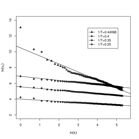
Figure 1: The log-log distribution of the domain masses $x_{k}$ versus the rank order index $k$ for the two-dimensional Ising model for $T=2.2692$(the critical temperature) ($\Diamond$),$T=2.5000$ ($\ast$), $T=2.8571$ ($\Box$) and $T=4.0000$ ($\circ$) for $L=1000$.

The straight lines with the slopes near $-1/\mu$ are given in Table 1, correspond to temperatures greater than the critical temperature $T_{c}$ ($T_{c}=2.2692$).

Table 1: The estimation of indexes $\mu$ with standard deviations $s$.

$T$	$\mu$	$s$
$4.0000$	$6.7136$	$0.0477$
$2.8571$	$4.7018$	$0.0603$
$2.5000$	$3.8240$	$0.0695$
$T_{c}\simeq 2.2692,\quad$	$0.9854$	$0.0874$

The estimations of the indexes $\mu$ for the two-dimensional Ising model with different temperatures based on 1000 realisations for $L=1000$ lattice are presented in Table 1. and Fig. 1.
It is seen from Fig. 1. that a slope $arctan(1/{\mu})$ of the line only for the critical temperature is near $\pi/4$ for the critical temperature and the Zipf law is satisfied. For the temperatures above critical temperature, slopes are smaller than $\pi/4$ and the Zipf law is not valid. One can notice that the validity of the Zipf law when the phase transition is present is in agreement with the relation $1/\mu=|2H-1|$ Czi , where $H$ is the Hurst exponent.It is well known that the system exhibits infinite long correlations at the critical point,which corresponds to the biggest value of the Hurst exponent.In such a case one obtains $\mu=1$.
The Pareto distribution implies the Zipf law Tro ,Klt ,but not inversally - for instance the Zipf law is satysfied also in the case of the hyperbolic distributionsHar .
The probability density of the Pareto distributions is defined as follows:

$$\rho(x)=(\mu/x_{0})(x{{}_{0}}/x)^{\mu+1}$$ (5)

for $x>x_{0}$, where $x_{0}$ denotes a typical scale.

One can define so called $\mu$-variableBou ,Bou1 .The main property of $[\mu]$-variable is that all its moments $m_{q}=<X^{q}>$ with $q\geq\mu$ are infinite. The question in classic probabilistic theory answered by Lévy and Khintchine shows how to characterize the limit distribution of the sum of N independent random variables $x$. Suppose that $\rho(x)$ decreases for a large x such as $x^{-1-\mu}$, then considering power-law distributions we can distinquish the following ranges for the critical exponents $\mu$ :

(i)For $\mu>2$, the moment of the first order $m_{1}$ and the moment of the second order $m_{2}$ are finite.
For this range of $\mu$,the two parameters $m_{1}$ and $m_{2}$ are finite and for large N the central limit theorem applies and the statistical distribution of the system tends towards a Gaussian distribution.
( ii)For $1<\mu<2$ only the moment of the first order is finite but the moment of the second order is infinite.
(iii) For $\mu<1$ the moments of the first and the second order are infinite.For a large number of elements of the system it is described according to the Lévy stable distribution, for instance the Pareto distribution.
But magnetic domains described by the clusters of the Ising or the Potts models are not independent variabes. Although we do not have a correspondence between $\mu$ and the slope of distributions described in (i)-(iii), respectively, the presence of the Pareto-type dystrybutions are also possible in the case of the dependent variables .

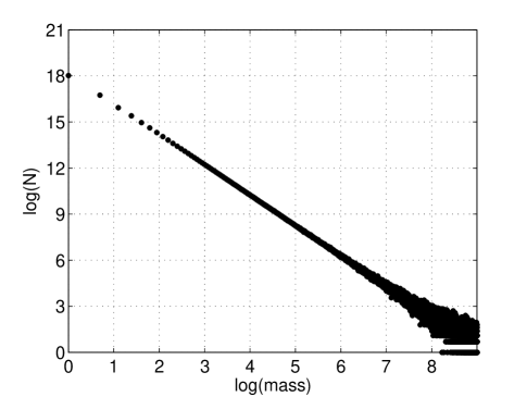
Figure 2: The dependence between the number of domains with mass x normalizedby the number of configurations $(N_{x}/N)$ from the mass $(x)$in the log-log scale, for the two dimensional Ising model near the criticalpoint $T_{c}$, for $10000$ configurations and $L=600$.

The straight line of Fig. 2 presents the Pareto distribution.

In our case, away from the criticality, the Gaussian-type distributions are not present when $\mu>2$. In this region the range of lengths, where the system is fractal, it is limited by the finite correlation length and the power-law tail in the distribution is suppressed.

Fig. 3 presents the distributions of the number of configurations with defined mass.The total number of configurations is $10000$.Histograms are presented for masses $x=5$, $x=10$, $x=50$ and$x=70$ for , for a system with $L=600$, beyond the phase transition inverse temperature $\beta=0.25$.

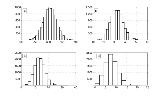
Figure 3: Histogram of the fixed domain mass $m=5$(a),$m=10$(b), $m=50$(c) and $m=70$(d) for the inverse temperature $\beta=025$, for the system with $L=600$, for $10000$ configurations.

The test for the Gaussian distribution was performed using the Kolmogorow-Smirnov method and the chi-square test. The Gaussian distributions for the number of clusters of a fixed size are present only for the masses smaller than 5. For example for the temperature $T=4.000$ and the cluster of size 5 the p-value of the chi-squared test was equal to$0.0771$.For the clusters of larger size we obtain the right-skewed distributions.

Fig. 4 presents the distribution of the number of configurations with a defined mass.The total number of configurations is $10000$.Histograms are presented for masses $x=5$, $x=10$, $x=50$ and $x=70$ for ,for a system with $L=600$ near critical point ($T_{c}=2.2692$).

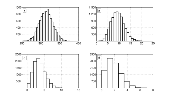
Figure 4: Histogram of the fixed mass $m=5$(a), $m=10$(b), $m=50$(c) and $m=70$(d) for the critical temperature, for the system with $L=600$, for 10000 configurations.

In this case the right-skewed distributions are present.The Gaussian distributions we observe only for masses smaller than 3. For example for the cluster of size 5 the p-value of the chi-square test was equal to 0.01174.

The main conclusion from this paper is following: In the critical region the Zipf law is satisfied and the power law distributions, the Pareto distributions are present.The histograms of the numbers od domain configurations,which possess the same number of domains present the right-skewed distributions mainly, for the critical point as well beyond it. The Gaussian-type distributions appear only for small masses .

References

- (1) G.H.Zipf,Human Behaviour and the Principle of Least effort Cambridge,MA:Addison-Wensley,1949.
- (2) M.Batty, Hierarchy in Cities and City Systems,CASA UCL London,2004
- (3) J.P.Bouchaud, Workshop on Levy Flights and Related Topics in Physics(Nicea,France 27-30 June 1994)ed.M.F.Shlesinger,G.M.Zasławsky(Berlin-Springer).
- (4) S.Wuchty,Mol.Biol.Evol.18 (2001),1694.
- (5) Y.G.Ma,Phys. Rev.Lett.83(1999),3617.
-
(6)
A.Sicilia,J.J.Arenzon,I.Dierking,A.J.Bray,L.F.Cugliandolo,
J.Martinez-Perdiguero,I.Alonso, I.C.Pintre,Phys.Rev.Lett.101,197801(2008). - (7) J.Cardy and R.M.Ziff,Journal of Statistical Physics,110(2003).
- (8) K.Lukierska-Walasek,K.Topolski,Rev.Adv.Matter Sci.23(2010)141.
-
(9)
K.Lukierska-Walasek,K.Topolski,Comp.Meth.Techn.16,
173(2010). - (10) A.Cognilio,W.Klein,J.Phys.13,2775(1980).
- (11) W.Janke,A.M.J.Schakel,Phys.Rev.E71, 0367039(2005)
- (12) Marco D’onorio De Meo,Dieter W.Heermann,Kurt Binder, J.Stat. Phys.60,585(1990).
- (13) R.Swendsen,J.Wang,Phys.Rev.lett.58,86( 1986).
- (14) B.B.Mandelbrot,The Fractal Geometry of the Nature,(W.H.Freeman and Company, New York 1983)
-
(15)
A.Czirok,R.Mantegna,S.HavlinandH.E.Stanley,
Phys.Rev.E52,446,(1995). - (16) J.P.Bouchaud,A.Georges, Physics Reports195,127(1995).
- (17) G.Troll,P.Beim Graben, Phys.Rev.E57,1347(1998).
- (18) P.Harremoes,F.Topsoe,Entropy3, 191(2001).