Worldline techniques and QCD observables

Abstract

This report attempts to capture the essential workings of gauge links (Wilson lines) inside gauge-invariant formulations of parton distribution functions in QCD and gain some deeper insight into their key (renormalization) properties. We show, in particular, that the one-loop anomalous dimension of the Cherednikov-Stefanis quark TMD PDF is in the lightcone gauge $A^{+}=0$, combined with the Mandelstam–Leibbrandt pole prescription, the same as that obtained in the special covariant gauge $a=-3$, leaving no uncanceled rapidity singularities.

11.15.-q, 11.10.Gh, 12.38.Aw, 12.39.St

1 Introduction

The standard way to remove the gauge-dependence of nonlocal correlators in gauge theories, like QCD, is to include path-ordered exponential factors of the gauge field that are absent in the original Lagrangian of a local quantum field theory. These operators are in general contour-dependent and give rise to new divergences, called in modern jargon rapidity divergences, that are not related to the standard singularities — ultraviolet (UV) and infrared (IR) — that appear in Feynman diagrams. They originate from contour irregularities caused by topological obstructions — endpoints, cusps, self-crossings — of the gauge contours entering the exponents of the gauge links and affect the renormalization properties of the QCD correlators [1]. The trouble is, such divergences have to be regularized and there is great ambiguity in adopting an appropriate subtraction procedure within a valid factorization scheme. Moreover, the use of the lightcone gauge quantization depends crucially on the adopted boundary conditions imposed on the gluon propagator in order to treat the gauge links at infinity.

These issues will be considered here in some detail. In Sec. 1, we will address the one-loop virtual corrections of the quark propagator in a general covariant gauge within two different gauge-invariant schemes: The Mandelstam formalism [2] and the $z$-field algorithm [3, 4]. Then, in Sec. 3, we will discuss — as an example of a transverse-momentum dependent (TMD) parton distribution function (PDF) — the quark in a quark TMD PDF, $f_{q/q}$, using the lightcone gauge subject to various boundary conditions on the gluon propagator. Finally, the conclusions will be presented in Sec. 4.

2 Mesonic correlator

In this section, we consider a gauge-invariant mesonic type correlator in QCD, viz.,

$$M(x_{1},x_{2}|\Gamma)=\bar{q}_{i}(x_{2})[x_{2},x_{1}|\Gamma]_{ij}q_{j}(x_{1})\,,$$ (1)

where

$$[x_{2},x_{1}|\Gamma]_{ij}=\mathcal{P}\exp\left[ig\int_{x_{1}[\Gamma]}^{x_{2}}dz_{\mu}A_{a}^{\mu}(z)t_{ij}^{a}\right]$$ (2)

is a path-ordered gauge link along some arbitrary contour $\Gamma$ between $x_{1}$ and $x_{2}$ and $t_{ij}^{a}=(1/2)\lambda_{ij}^{a}$ are the Gell-Mann matrices of $SU(3)_{c}$. In principle, any contour between the points $x_{1}$ and $x_{2}$ is admissible. Contour obstructions give rise to rapidity divergences and hence contribute to the anomalous dimension of the correlator. For our considerations in this section, we assume that the contour is smooth. Because only the two endpoints entail rapidity divergences, it is sufficient to employ the straight line $\bar{\Gamma}$ joining $x_{1}$ and $x_{2}$. The reason is that other features of smooth contours, e.g., their length, do not affect the renormalization properties of the twist-two mesonic correlator and hence $\bar{\Gamma}$ can be used as a subtraction contour for its renormalization for all members of the universality class of smooth contours. Differences in the definition of the mesonic correlator for different smooth contours show up at the next higher twist level [5].

The gauge link can be treated in two different ways. One can evaluate the path-ordered exponential as a power series in the coupling using the Mandelstam formalism [2]. This approach [6] will be on focus in the first subsection below. Another option is to apply the $z$-field algorithm [3, 4], which is based on an effective Lagrangian describing the interaction of one-dimensional auxiliary Fermion fields with the gluon field and trade contours for “particle trajectories”. Fully quantized results are finally obtained by performing a functional integral over the $z$-field fluctuations to get the mesonic correlator in second quantization. Our presentation here follows the analysis of [7] with more details to be given in a future publication.

2.1 Mandelstam formalism

We carry out the vacuum expectation value of $M(x_{1},x_{2}|\Gamma)$ to the second order of the unrenormalized coupling constant $g$, i.e.,

$$\langle 0|T\left(\bar{q}(x_{2})[x_{2},x_{1}|\Gamma]q(x_{1})\right)\!|0\rangle^{(2)} \!\!=\!\! \langle 0|T\left(\bar{q}(x_{2})[x_{2},x_{1}|\Gamma]q(x_{1})\right)\!|0\rangle^{(2)}$$ (3)

$$\!\!+\langle 0|T\left(\bar{q}(x_{2})[x_{2},x_{1}|\Gamma]^{(1)}q(x_{1})\right)\!|0\rangle^{(1)}$$

$$\!\!+\langle 0|T\left(\bar{q}(x_{2})[x_{2},x_{1}|\Gamma]^{(2)}q(x_{1})\right)\!|0\rangle^{(0)}$$

with each contribution evaluated to the appropriate order. The first term is the usual gauge-dependent quark self-energy to $\mathcal{O}(g^{2})$, whereas the second and the third term represent the $\mathcal{O}(g^{1})$ and the $\mathcal{O}(g^{2})$ contributions stemming from the gauge link (termed in [6] the connector), respectively:

$$[x_{2},x_{1}|\Gamma]^{(1)} = ig\int_{x_{1}[\Gamma]}^{x_{2}}dz_{\mu}A^{\mu}(z)\ ,$$ (4)

$$[x_{2},x_{1}|\Gamma]^{(2)} = \frac{(ig)^{2}}{2!}\int_{x_{1}[\Gamma]}^{x_{2}}dz_{\mu}\int_{x_{1}[\Gamma]}^{x_{2}}dz_{\nu}^{\prime}\mathcal{P}\left(A^{\mu}(z)A^{\nu}(z^{\prime})\right)\ .$$ (5)

The three terms displayed in Eq. (3) are shown graphically in Fig. 1.

          

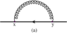
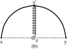
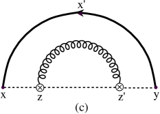
Figure 1: One-loop contributions to the vacuum expectation value of the mesonic correlator in Eq. (3) within the Mandelstam formalism. (a) Usual quark self-energy with gluon attachment denoted by a curly line; (b) and (c) contributions due to Eqs. (4) and (5), respectively. Curved solid lines denote quark propagators, whereas the gauge contours are represented by dashed straight lines with the symbol $\otimes$ denoting line integrals along them.

It was shown in [6] that the rapidity divergences entailed by the endpoints in diagrams (b) and (c) in Fig. 1 can be controlled by dimensional regularization with no need to involve additional regulators. The explicit calculation can be found there. Here we only quote the final results recalling that we are dealing with quark fields that are Heisenberg field operators in the interaction picture (where they are free operators) so that one has to perform all Wick contractions in

$$\mathcal{M}(x_{1},x_{2}|\Gamma)=\left\langle 0\left|T\!\left(\bar{q}_{0}(x_{2})[x_{2},x_{1}|\Gamma]q_{0}(x_{1})\exp\left(\!i\!\int d^{4}y\mathcal{L}_{\rm int}(y)\right)\!\right)\right|0\right\rangle.$$ (6)

The mesonic correlator in a general covariant gauge $a$ can be written in the form

$$\mathcal{M}^{(i,j)}(p|\bar{\Gamma})=\mathcal{M}_{1}^{(a,b)}(p)+(1-a)\mathcal{M}_{2}^{(a,b)}(p)$$ (7)

with

$$D_{\rm F}^{\mu\nu}(k)=-\frac{g^{\mu\nu}}{k^{2}+i\epsilon}+(1-a)\frac{k^{\mu}k^{\nu}/k^{2}}{k^{2}+i\epsilon}\ ,\quad S_{\rm F}(p)=\frac{1}{\hat{p}-m+i\epsilon}\ ,$$ (8)

where the first superscript in $\mathcal{M}^{(i,j)}$ indicates the order of the expansion of the gauge link, whereas the second one denotes the order of the coupling taken into account in the Wick contractions. One finds [6] that the connector parts are interrelated: $\mathcal{M}_{2}^{(1,1)}(p)=-2\mathcal{M}_{2}^{(2,0)}(p),$ while the remaining part of $\mathcal{M}_{2}^{(1,1)}(p)$ cancels the $(1-a)$ contribution of $\mathcal{M}_{2}^{(0,2)}(p),$ so that $\mathcal{M}^{(2)}(p|\bar{\Gamma})$ is gauge-parameter independent and multiplicatively renormalizable:

$$\mathcal{M}(p|\bar{\Gamma})|_{\rm ren}=Z_{\rm hybrid}^{-1}\mathcal{M}(p|\bar{\Gamma})|_{\rm bare}\ .$$ (9)

Using dimensional regularization we obtain in the $\overline{\rm MS}$ scheme the following renormalization constants ($D=4-\epsilon$) [6]

$$Z_{\rm hybrid} = Z_{2q}Z_{\rm con}=1+\frac{3g^{2}}{8\pi^{2}}C_{\rm F}\frac{1}{\epsilon}+\mathcal{O}(g^{4})$$ (10)

$$Z_{\rm con} = 1+\frac{g^{2}}{8\pi^{2}}C_{\rm F}(3+a)\frac{1}{\epsilon}+\mathcal{O}(g^{4})\ ,\quad$$ (11)

$$Z_{2q} = 1-\frac{g^{2}}{8\pi^{2}}C_{\rm F}a\frac{1}{\epsilon}+\mathcal{O}(g^{4})\ ,$$ (12)

where $C_{\rm F}=(N_{c}^{2}-1)/(2N_{\rm c})=4/3$ for $N_{\rm c}=3$ The associated anomalous dimensions ($\gamma=\frac{1}{2}\mu\frac{\partial}{\partial\mu}\ln Z$) are given by

$$\gamma_{\rm hybrid} = \gamma_{2q}+\gamma_{\rm con}=-\frac{3g^{2}}{16\pi^{2}}C_{\rm F}+\mathcal{O}(g^{4})$$ (13)

$$\gamma_{\rm con} = -\frac{g^{2}}{16\pi^{2}}C_{\rm F}(3+a)+\mathcal{O}(g^{4})\ ,\quad$$ (14)

$$\gamma_{2q} = \frac{g^{2}}{16\pi^{2}}C_{\rm F}a+\mathcal{O}(g^{4})$$ (15)

and bear no dependence on the geometric features of the contour, e.g., its length or its derivatives $d^{n}x(\tau)/(d\tau)^{n}$.

2.2 $z$-field formalism

Though the correlator $\mathcal{M}(x_{1},x_{2}|\Gamma)$ is multiplicatively renormalizable, it cannot be written contour-independently in the factorized form $M(x_{1},x_{2}|\Gamma)=\bar{Q}(x_{2}|\Gamma_{2})Q(x_{1}|\Gamma_{1})$ starting from the QCD Lagrangian in terms of the Mandelstam field $Q(x_{1}|\Gamma_{1})=\mathcal{P}\exp\left[ig\int_{-\infty[{\Gamma_{1}}]}^{x_{1}}dz_{\mu}A_{a}^{\mu}(z)t_{a}\right]q(x_{1}).$ However, for smooth contours one can factorize the connector $[x_{1},x_{2}|\Gamma]$ according to the algebraic identity $[B,A|\Gamma]=[B,C|\Gamma_{2}][C,A|\Gamma_{1}]$ with $\Gamma_{1}\cup\Gamma_{2}=\Gamma$ and then shift $C\to\infty$. This trick allows factorization and multiplicative renormalization, i.e., $Q(x|\Gamma)|_{\rm ren}=Z_{\rm hybrid}^{-1/2}Q(x|\Gamma)|_{\rm bare}.$

Figure 2: One-loop contributions to the mesonic correlator in the $z$-field formalism: (a) $z$-field (broken line) self-energy; (b) and (c) vertex corrections from $\bar{z}A^{\mu}\frac{dx_{\mu}(\sigma)}{d\sigma}z$.

A more far-sighted option is to trade gauge contours in favor of “trajectories” of fictitious particles described by the following effective Lagrangian

$$\mathcal{L}_{\rm eff}=\int_{0}^{1}d\sigma\left[\bar{z}(\sigma)\frac{\partial}{\partial\sigma}z(\sigma)+ig\bar{z}(\sigma)\frac{dx_{\mu}(\sigma)}{d\sigma}A^{\mu}(x(\sigma))z(\sigma)+i\bar{\lambda}z+i\bar{z}\lambda\right]$$ (16)

and supplement $\mathcal{L}_{\rm QCD}$ by two additional terms pertaining to two extra Feynman rules: one for the $z$-field propagator and the other for the $z$-field–gluon vertex (see [7]). This allows one to write the gauge link as a path integral:

$$\mathcal{P}\exp\left[ig\int_{\sigma_{1}}^{\sigma_{2}}d\sigma A_{a}^{\mu}(x(\sigma))t^{a}\frac{dx_{\mu}}{d\sigma}\right]_{ij}\equiv\langle 0|z_{i}(\sigma_{2})\bar{z}_{j}(\sigma_{1})|0\rangle\ ,$$ (17)

where $\langle\mathcal{Q}\rangle=\int\mathcal{D}\bar{z}\mathcal{D}z\mathcal{Q}\exp\left[\int_{\sigma_{1}}^{\sigma_{2}}d\sigma\bar{z}(\sigma)D_{\sigma}z(\sigma)\right].$ What is more, performing now the calculation of the radiative corrections to the mesonic correlator within this approach (see Fig. 2), one finds at $\mathcal{O}(g^{2})$ that the local combination $\bar{z}(\sigma_{x})q(x)$ (analogous to the nonlocal field $Q(x|\Gamma)$ in the Mandelstam formalism) gets renormalized by the renormalization constant [7] $Z_{\rm CF}^{-1/2}=\tilde{Z}_{\rm CF}^{-1/2}Z_{2q}^{-1/2}Z_{3z}^{1/2},$ where $Z_{3z}=1+\frac{g^{2}}{8\pi^{2}}C_{\rm F}(3-a)\frac{1}{\epsilon}$ resembles $Z_{\rm con}$, yielding to the same anomalous dimensions as before. As a result, the Slavnov-Taylor identities to $\mathcal{O}(g^{2})$ are fulfilled ($C_{\rm A}=N_{\rm c}=3$):

$$\frac{Z_{\rm con}Z_{1q}}{Z_{\rm hybrid}}=\frac{Z_{3}}{Z_{1}}=\frac{\tilde{Z}_{3}}{\tilde{Z}_{1}}=\frac{Z_{3z}}{Z_{1z}}=1+\frac{C_{\rm A}g^{2}}{32\pi^{2}}(3+a)\frac{1}{\epsilon}\ .$$ (18)

One can now use the $z$-field formalism and perform a short-distance expansion of $M(x_{1},x_{2}|\Gamma)$ for $x_{1}\longrightarrow x_{2}$:

$$M(x_{1},x_{2}|\Gamma) = \bar{q}(x_{2})[x_{2},x_{1}|\Gamma]q(x_{1})=\bar{q}(x_{2})z(\sigma_{2})\bar{z}(\sigma_{1})q(x_{1})$$

$$\approx \sum_{N,i}C_{N}^{(i)}(z^{2},g,C)z^{\mu_{1}}\ldots z^{\mu_{N}}\mathcal{O}_{z^{\mu_{1}}\ldots z^{\mu_{N}}}^{(i)}(x,C)\ ,$$

where $(x_{2}-x_{1})^{2}=z^{2}\simeq 0$, $z^{\mu}\neq 0$ and the composite non-singlet quark operator of lowest twist reads

$$\mathcal{O}_{z^{\mu_{1}}\ldots z^{\mu_{N}}}^{(i)}(x,C)=\bar{q}(x)\gamma_{\mu_{1}}\overleftrightarrow{D}_{\mu_{1}}\ldots\overleftrightarrow{D}_{\mu_{N}}[x,x|C]q(x)\ .$$ (20)

Here $[x,x|C]$ is a gauge link along the closed loop $C=\Gamma\cup\Gamma^{\prime}$ and the short-distance expansion is valid for any point $x$ because the smooth contour $\Gamma^{\prime}$ can be stretched to $\infty$ by virtue of the independence of the renormalization constants on $L(\Gamma^{\prime})$. An immediate important conclusion is that in the special gauge $a=-3$ all contour- (or $z$-field-) related divergences cancel among themselves so that the residual renormalization effects can be absorbed into $Z_{3}$, while the Ward identity $Z_{1q}=Z_{2q}$ is preserved like in QED. It is expected that going to the next higher loop, one will obtain a similar result but for $a^{*}=-3+\mathcal{O}(g^{2})$ as found in [8] in the context of multiloop contributions to the nonsinglet QCD evolution equations.

3 Gauge-invariant correlators for TMD PDFs

With such issues in mind, let us focus attention on the question of the appropriate definition of a TMD PDF (e.g., [9] and references cited therein). In [10] we have shown that $f_{q/q}(x,\bm{k}_{\perp})$ given in [11] cannot be regularized completely using dimensional regularization in the lightcone gauge $A^{+}=(A\cdot n^{-})=0$ with $(n^{-})^{2}=0$ in conjunction with the retarded (ret), advanced (adv), or principal-value (PV) pole prescription on the gluon propagator:

$$D_{\mu\nu}^{\rm LC}(q)=\frac{-i}{q^{2}-\lambda^{2}+i0}\left(g_{\mu\nu}-\frac{q_{\mu}n^{-}_{\nu}+q_{\nu}n^{-}_{\mu}}{[q^{+}]}\right)\ ,$$ (21)

where

$$\frac{1}{[q^{+}]}\Bigg{|}_{\rm Ret/Adv}=\frac{1}{q^{+}\pm i\eta}\ \ \ ,\ \ \ \frac{1}{[q^{+}]}\Bigg{|}_{\rm PV}=\frac{1}{2}\left[\frac{1}{q^{+}+i\eta}+\frac{1}{q^{+}-i\eta}\right]\ .$$ (22)

The reason is that the residue of the $\epsilon$ pole contains a rapidity divergence that entails an extra anomalous dimension and calls for an additional subtraction procedure. This can be achieved in terms of a soft factor $R$ that has to be included into the definition of the TMD PDF [10]. Its anomalous dimension $\gamma_{R}$ serves to cancel $\delta\gamma$ with the effect that the anomalous dimension of $f_{q/q}^{R}$ coincides with the result one would obtain in a covariant gauge for a direct smooth contour between the two field points i.e., Eq. (13). It turns out [10] that this anomalous-dimension artifact has at one loop the same structure as the universal anomalous dimension of a cusped contour [12], $\delta\gamma=-\frac{\alpha_{s}}{\pi}C_{\rm F}\ln\frac{\eta}{p^{+}},$ which becomes infinite when $\eta\to 0$. For such $q^{-}$-independent pole prescriptions the gluon propagator is not transverse: $n_{\mu}D^{\mu\nu}\neq 0$. On the other hand, it was shown in [13] that using instead the $q^{-}$-dependent Mandelstam–Leibbrandt (ML) [14] pole prescription

$$D_{\rm ML}^{\mu\nu}(q^{2})=\frac{i}{q^{2}}\left[-g^{\mu\nu}+\frac{q^{\mu}n^{\nu}+q^{\nu}n^{\mu}}{[q^{+}]}\right];~{}~{}~{}\frac{1}{[q^{+}]_{\rm ML}}=\left\{\begin{array}[]{ll}&\!\!\!\!\!\!\!\frac{1}{q^{+}+i0q^{-}}\\ &\!\!\!\!\!\!\!\frac{q^{-}}{q^{+}q^{-}+i0}\end{array}\right.$$ (25)

one has $n_{\mu}D_{\rm ML}^{\mu\nu}=0$. The opposite claims by Collins in [15] are likely the result of misunderstanding, as his equation (15) shows the gluon propagator subject to the Principal Value pole prescription, i.e., Eq. (22). This gluon propagator is indeed not transverse. The same applies to those obtained with the advanced or retarded pole prescription, because in all these cases the transverse gauge field $\mathbf{A}^{\perp}(\infty^{-};\bm{\xi}_{\perp})=\frac{g}{4\pi}C_{\infty}\bm{\nabla}^{\perp}\ln\Lambda|\bm{\xi}_{\perp}|$ is not purely transverse (in contrast to the ML case) but depends through $C_{\infty}=\{0(\rm adv),-1(ret),-\frac{1}{2}(PV)\}$ on the imposed boundary conditions.

Another issue raised by Collins in [15] is whether the definition of $f_{q/q}^{R}$ contains uncanceled divergences originating from the self-energy of the gauge links. We have shown in [10, 13] that all UV divergences from the $q$ momentum integrations can be regularized dimensionally and give $1/\epsilon$ poles, while collinear poles are controlled by the quark virtuality $p^{2}<0$, and IR singularities are regularized by an auxiliary gluon mass $\lambda$ that drops out at the end. On the other hand, overlapping divergences have, in general, to be cured by a subtraction procedure encoded in the soft renormalization factor $R$ and appear in $\ln\frac{\eta}{p^{+}}$ in terms of an auxiliary mass $\eta$. In the $A^{+}=0$ gauge all diagrams with gluon attachments to the gauge links (longitudinal or transverse) either vanish identically or cancel partly against contributions from cross-talk diagrams with gluon attachments between the quark line and a gauge link. For the adv, ret, and PV pole prescriptions, all remaining divergences are taken care of by the soft factor rendering $f_{q/a}^{R}$ regular. Employing the ML prescription, one gets a result that is reminiscent of that obtained in the special covariant gauge $a=-3$ in which all rapidity divergences emerging from the endpoints of smooth contours cancel among themselves. At higher loops, the gauge $a=-3$ will receive $\alpha_{s}$ corrections with coefficients that can be determined by demanding the validity of the QED-like Ward identity $Z_{1q}=Z_{2q}$.

4 Conclusions

We have shown the multiplicative renormalization of the gauge-invariant mesonic vacuum correlator in the nonlocal Mandelstam approach for smooth contours and found that to $\mathcal{O}(g^{2})$ it is equivalent to the result obtained in the local $z$-field effective formalism. At one loop, all contour- (or $z$-field) related rapidity divergences cancel among themselves using the special gauge $a=-3$. We argued that a proper definition of the quark TMD PDF must account for the appropriate subtraction of a rapidity divergence that overlaps with the usual UV singularities and cannot be regularized dimensionally. Employing the lightcone gauge with $q^{-}$-independent pole prescriptions, this can be achieved via a soft renormalization factor [10]. The imposition of the $q^{-}$-dependent Mandelstam–Leibbrandt prescription removes all rapidity divergences and reproduces at one loop the results of the special covariant gauge $a=-3$ with the soft factor reducing to unity.

References

- [1] A.M. Polyakov, Nucl. Phys. B164, 171 (1979).
- [2] S. Mandelstam, Phys. Rev. 175, 1580 (1968).
- [3] M.B. Halpern, A. Jevicki, P. Senjanovic, Phys. Rev. D16, 2476 (1977).
- [4] J.-L. Gervais, A. Neveu, Nucl. Phys. B163, 189 (1980).
- [5] I.O. Cherednikov, A.I. Karanikas, N.G. Stefanis Nucl. Phys. B840, 379 (2010).
- [6] N.G. Stefanis, Nuovo Cim. A83, 205 (1984).
- [7] N.S. Craigie, H. Dorn, Nucl. Phys. B185, 204 (1981).
- [8] S.V. Mikhailov, Phys. Rev. D62, 034002 (2000); Phys. Lett. 431, 387 (1998).
- [9] J.C. Collins, T.C. Rogers, arXiv:1210.2100 [hep-ph].
- [10] I.O. Cherednikov, N.G. Stefanis, Phys. Rev. D77, 094001 (2008); Nucl. Phys. B802, 146 (2008); N.G. Stefanis, I.O. Cherednikov, Mod. Phys. Lett. A24, 2913 (2009).
- [11] A.V. Belitsky, X. Ji, F. Yuan, Nucl. Phys. B656, 165 (2003).
- [12] G.P. Korchemsky, A.V. Radyushkin, Nucl. Phys. B283, 342 (1987).
- [13] I.O. Cherednikov, N.G. Stefanis, Phys. Rev. D80, 054008 (2009).
- [14] S. Mandelstam, Nucl. Phys. B213, 149 (1983); G. Leibbrandt, S.L. Nyeo, Phys. Lett. B140, 417 (1984).
- [15] J.C. Collins, Int. J. Mod. Phys. Conf. Ser. 4, 85 (2011).