Concise Quantum Associative Memories with Nonlinear Search Algorithm

Abstract

The model of quantum associative memories (QAM) we propose here consists in simplifying and generalizing that of Rigui Zhou et al. [1] who uses the quantum matrix with the binary decision diagram put forth by David Rosenbaumand [2] and the Abrams and Lloyd’s nonlinear search algorithm [3]. Our model gives the possibility to retrieve one of the sought states in multi-values retrieving scheme when a measure on the first register is done in $\mathcal{O}(c-r)$ time complexity. It is better than Grover’s algorithm and its modified form which need $\mathcal{O}(\sqrt{\frac{2^{n}}{m}})$ steps when they are used as the retrieval algorithm. $n$ is the number of qubit of the first register and $m$ the number of values $x$ for which $f(x)=1$. As the nonlinearity makes the system highly susceptible to noise, an analysis of the influence of the single qubit noise channels on the Nonlinear Search Algorithm of our model of QAM, shows a fidelity of about $0.7$ whatever the number of qubits existing in the first register.

1 Introduction

Quantum Neural Networks are Artificial Neural Networks functioning according to quantum laws. One of the useful Neural Networks is the Associative Memory which is an important tool for pattern recognition, intelligent control and artificial intelligence. Ventura and Martinez have built a model of Quantum Associative Memory (QAM) where the stored patterns are considered as the basis states of the memory quantum state [4]. They used a modified version of the well-known Grover’s quantum search algorithm in an unsorted database as the retrieval algorithm. In order to overcome the limits of that model to only solve the completion problem by doing data retrieving from noisy data, Ezhov et al. have used an exclusive method of quantum superposition and Grover’s algorithm with distributed queries [5] . However, their model still produces non-negligible probability of irrelevant classification. We have recently put forth an improved model of QAM with distributed query that reduces the probability of this irrelevant classification [6].

The NonLinear Search Algorithm (NLSA) is based on the fact that it has been suggested that under some circumstances, the superposition principle of quantum theory might be violated. In other words, sometime a quantum system might have temporal nonlinear evolution. Therefore, nonlinear quantum computer could solve NP-complete and even #P problems in polynomial time that Abrams and Lloyd argued in 1998 in their nowadays classic paper [3]. We recall that the NLSA of Abrams and Lloyd uses the Weinberg’s prescription and they based their argument on a general property of nonlinear evolutions in Hilbert spaces. This nonlinear evolution is the non-conservation of scalar products between nonlinearly evolving solutions of a nonlinear Schrödinger equation. This effect is called a mobility phenomenon. In order to avoid the fact that the Weinberg’s formalism imply faster than light transmission [8], Czachor [7] has proposed another description, based on the Polchinski-type one. The state components evolution depend upon hyperbolic tangents. In the present paper, we follow the Czachor’s description. Meyer and Wong give in [9] another reason which can justify the use of nonlinear formalism in quantum mechanics:

“[…] An obvious question is whether a modest, physically motivated nonlinearity can still produce a computational advantage. In particular, consider Bose-Einstein condensates (BECs). […] In general, describing such many-body systems is difficult because of the many interaction terms. But under certain conditions, one can assume that only two-body contact interactions contribute and the s-wave scattering length $a$ is much less than the interparticle spacing. Then using mean field theory, one finds that the system is approximately described by a nonlinear Schrödinger equation […]”

Therefore, Meyer and Wongthey have used Gross-Pitaevskii equation to build their nonlinear search algorithm.

Rigui et al. [1] have recently proposed a model of Ventura’s associative memory which uses Binary Superposed Quantum Decision Diagram (BSQDD) as a learning process. They also used the above nonlinear algorithm of Abrams and Lloyd as a retrieving process for multi-values retrieval. Although the learning process of their model is good, there is some ambiguities on how the memory evolves and how the multi-values retrieval arises. First of all, there is no exact description about operator $U_{1}$ which links the first register denoted by ${\left|{\psi_{i}}\right\rangle}$ to the second register denoted by ${\left|{\gamma}\right\rangle}$. Secondly the use of simple binary decision diagram to represent states ${\left|{\Phi}\right\rangle}$ (see step 2 on section 3.2) seems to only show the way to attempt the needed state. Moreover the nonlinear operator denoted by $U_{3}$ seems to be use on particular state, not on supposed state (see step 3 on section 3.3 and section 4.2 in [1]). There is also no indication on how a measure will give a needed state according to the fact that nonlinear search algorithm leaves the first register in a superposed state.

In this paper, as the primary innovation, we propose a concise NLSA for QAM with a method to retrieve one of the sought states, especially in multi-values retrieving scheme when a measure is done only on the first register with $\mathcal{O}(c-r)$ time complexity. The parameters $c$ and $r$ are obtained as follow. If $n$ is the number of qubits of first register, $p\leq 2^{n}$ the number of stored patterns and if the values of $t$ qubits are known (i.e., $t$ qubits have been measured or are already be disentangled to others, or the oracle acts on a subspace of $(n-t)$ qubits), then we have the number of stored patterns $q\leq p$ and the number of values $x$ for which $f(x)=1$ $m\leq q$. If $c=\mathtt{ceil}(\log_{2}{q})$ is the least integer greater or equal to $\log_{2}{q}$ and $r=\mathtt{int}(\log_{2}{m})$ the integer part of $\log_{2}{m}$. Thus, our model simplifies and generalizes that of Rigui et al. [1].

However, if the strength of the nonlinearity provides a large computational advantage, it also makes the system highly susceptible to noise which appears as a true bottleneck that may limit the usefulness of the NLSA. As another innovation of this paper, we investigate the effects of noise in the algorithm by considering the bit-flip quantum channel modeling environmentally induced noise. We assume that at most a single complete bit-flip error occurs on one of the data qubits. It should be noted that the problem of the influence of noise on the Grover quantum search algorithm has been extensively studied by various researchers [10, 11].

The paper is organized as follows: section 2 clearly describes the NLSA proposed by Abrams and Lloyd. Section 3 presents the QAM with NLSA, hereafter noted QAM-NLSA, with a new method to retrieve one of the sought states in multi-values retrieving scheme. In section 4, we introduce the single qubit noise channels model to the NLSA and we analyze its influence on our model of QAM. At the end, a short conclusion is provided in section 5. But we start with a short description of parameters used in this paper.

The following parameters will be used throughout the paper:

• $n$ is the number of qubit of the first register,

• ${\left|{z}\right\rangle}$ is the initial state of the first register,

• $x$ is the needed value while ${\left|{x}\right\rangle}$ is the corresponding state,

• $p\leq 2^{n}$ the number of stored patterns,

• $q\leq p$ the number of stored patterns if the values of $t$ qubits are known,

• $c=\mathtt{ceil}(\log_{2}{q})$, i.e. the least integer greater or equal to $\log_{2}{q}$,

• $m\leq q$ the number of values $x$ for which $f(x)=1$,

• $r=\mathtt{int}(\log_{2}{m})$ is the integer part of $\log_{2}{m}$.

2 Nonlinear search algorithm

Suppose there is a unitary transformation $\mathtt{U}_{f}$: the oracle or the black box which acts as follows: for a set of inputs between $0$ and $2^{n}-1$, there is at most one $x$ for which $f(x)=1$ and the other values give $0$. Let us consider two registers; the first register which is an $n$-qubit system is to compute inputs and the second which is a single-qubit system is to compute the answer of the oracle. We can define the function $f$ as

$$\begin{split}f:&\mathcal{H}^{\otimes n}\longrightarrow\mathcal{H}\\ &{\left|{y}\right\rangle}\longmapsto{\left|{\delta_{xy}}\right\rangle}\end{split}$$ (1)

where $\mathcal{H}^{\otimes n}$ is a Hilbert space of $2^{n}$ dimensions.

The nonlinear algorithm of Abrams and Lloyd aims to disentangle the flag qubit from the first register as a measure on the flag qubit can tell us if there is at most a value $x$ for which $f(x)=1$. This is done by transforming the part of the flag qubit that is ${\left|{0}\right\rangle}$ to ${\left|{1}\right\rangle}$. They claim that it is not possible to do by using linear operators of quantum information. The Abrams and Lloyd nonlinear algorithm is summarized by the Algorithm 1.

Algorithm 1 Nonlinear search algorithm (NLSA)

1:  Put the first register in the superposed state of all the $N$ values and the flag qubit to ${\left|{0}\right\rangle}$

2:  Apply the oracle $\mathtt{U}_{f}$

3:  for each qubit of the first register with the flag qubit do

4:      Apply the unitary operator $\mathtt{U}$

5:     

1. apply the nonlinear operator $\mathtt{NL}^{-}$

2. apply the nonlinear operator $\mathtt{NL}^{+}$

6:      Apply the Hadamard operator $\mathtt{W}$ on the qubit of the first register and the NOT operator $\mathtt{X}$ on the flag qubit

7:  end for

8:  Observe the flag qubit

Let ${\left|{\psi}\right\rangle}$ be the state which describes all the system and assume that all $N=2^{n}$ inputs are computed in the first register with equal amplitude:

$${\left|{\psi}\right\rangle}=\frac{1}{\sqrt{N}}\sum_{y}^{N}{\left|{y}\right\rangle}{\left|{0}\right\rangle}.$$ (2)

Applying the oracle yields

$$\begin{split}\mathtt{U}_{f}{\left|{\psi}\right\rangle}&=\frac{1}{\sqrt{N}}\sum_{y}^{N}{\left|{y}\right\rangle}{\left|{f(y)}\right\rangle}\\ &=\frac{1}{\sqrt{N}}\left(\sum_{y\neq x}^{N}{\left|{y}\right\rangle}{\left|{0}\right\rangle}+{\left|{x}\right\rangle}{\left|{1}\right\rangle}\right).\end{split}$$ (3)

To describe the disentanglement algorithm, we consider the binary forms of values and assume that there is at most one value $x$ which gives $f(x)=1$. Let ${\left|{j_{n}j_{n-1}\ldots j_{1}}\right\rangle}$ and ${\left|{i_{n}i_{n-1}\ldots i_{1}}\right\rangle}$ be the binary forms of states ${\left|{y}\right\rangle}$ and ${\left|{x}\right\rangle}$ respectively, with $j_{k},i_{k}\in\{0,1\}$. Equations (2) and (3) can be rewritten as

$${\left|{\psi}\right\rangle}=\frac{1}{\sqrt{2^{n}}}\left[\sum_{\begin{subarray}{c}j_{n}j_{n-1}\ldots j_{1}=0\\ j_{n}j_{n-1}\ldots j_{1}\neq i_{n}i_{n-1}\ldots i_{1}\end{subarray}}^{1}{\left|{j_{n}j_{n-1}\ldots j_{1}}\right\rangle}+{\left|{i_{n}i_{n-1}\ldots i_{1}}\right\rangle}\right]{\left|{0}\right\rangle},$$ (4)

and

$$\mathtt{U}_{f}{\left|{\psi}\right\rangle}={\left|{\Psi}\right\rangle}=\frac{1}{\sqrt{2^{n}}}\left[\sum_{\begin{subarray}{c}j_{n}j_{n-1}\ldots j_{1}=0\\ j_{n}j_{n-1}\ldots j_{1}\neq i_{n}i_{n-1}\ldots i_{1}\end{subarray}}^{1}{\left|{j_{n}j_{n-1}\ldots j_{1}}\right\rangle}{\left|{0}\right\rangle}+{\left|{i_{n}i_{n-1}\ldots i_{1}}\right\rangle}{\left|{1}\right\rangle}\right].$$ (5)

Highlighting the least significant qubit (LSQ) of the first register, equation (5) can be helpfully written as

$${\left|{\Psi}\right\rangle}=\frac{1}{\sqrt{2^{n}}}\left[\sum_{\begin{subarray}{c}j_{n}j_{n-1}\ldots j_{1}=0\\ j_{n}j_{n-1}\ldots j_{2}\neq i_{n}i_{n-1}\ldots i_{2}\end{subarray}}^{1}{\left|{j_{n}j_{n-1}\ldots j_{1}}\right\rangle}{\left|{0}\right\rangle}+{\left|{i_{n}i_{n-1}\ldots(1-i_{1})}\right\rangle}{\left|{0}\right\rangle}+{\left|{i_{n}i_{n-1}\ldots i_{1}}\right\rangle}{\left|{1}\right\rangle}\right].$$ (6)

The state (6) must be viewed as the general binary form of the system after the action of the oracle. It summarizes all particular states given by Czachor in [7] and removes ambiguities given by his notation. Indeed, his equation

$$\frac{1}{\sqrt{2^{n}}}\sum_{j_{n}j_{n-1}\ldots j_{2}=0}^{1}[{\left|{j_{n}j_{n-1}\ldots 0_{1}}\right\rangle}{\left|{1}\right\rangle}+{\left|{j_{n}j_{n-1}\ldots 1_{1}}\right\rangle}{\left|{0}\right\rangle}],$$ (7)

suggests that there is $2^{n-1}$ values $x$ for which $f(x)=1$, and not $s=1$ as he claims.

Considering the subsystem of only the LSQ of the first register ${\left|{\ell}\right\rangle}$ and the flag qubit ${\left|{k}\right\rangle}$, $k,\ell\in\{0,1\}$, the computer will be in one of the following states where we ignore the normalization constants,

$${\left|{00}\right\rangle}+{\left|{10}\right\rangle},$$ (8a)

$${\left|{10}\right\rangle}+{\left|{01}\right\rangle},$$ (8b)

$${\left|{00}\right\rangle}+{\left|{11}\right\rangle}.$$ (8c)

The left part of the equation (6) suggests that the state (8a) occurs with the highest probability whereas the state ${\left|{01}\right\rangle}+{\left|{11}\right\rangle}$ does not appear because the variable $x$ is supposed to be unique.

The nonlinear evolution (NLE), step 4 to step 6 of Algorithm 1, aims to transform the states (8b) and (8c) to ${\left|{01}\right\rangle}+{\left|{11}\right\rangle}$ while leaving the state (8a) unchanged. The NLE part of the algorithm then acts as follows:

• Apply the 2-qubit operator

  $$\mathtt{U}=\frac{1}{\sqrt{2}}\begin{pmatrix}1&0&0&1\\ 0&1&1&0\\ 0&1&-1&0\\ 1&0&0&-1\end{pmatrix}$$ (9)

  on the states (8):

  $$\mathtt{U}({\left|{00}\right\rangle}+{\left|{10}\right\rangle})=\frac{1}{\sqrt{2}}({\left|{00}\right\rangle}+{\left|{01}\right\rangle}-{\left|{10}\right\rangle}+{\left|{11}\right\rangle}),$$ (10a)

  $$\mathtt{U}({\left|{10}\right\rangle}+{\left|{01}\right\rangle})=\sqrt{2}{\left|{01}\right\rangle},$$ (10b)

  $$\mathtt{U}({\left|{00}\right\rangle}+{\left|{11}\right\rangle})=\sqrt{2}{\left|{00}\right\rangle}.$$ (10c)

• Apply the nonlinear 1-qubit operator $\mathtt{NL}^{-}$ on the flag qubit:

  $$\mathtt{NL}^{-}[\frac{1}{\sqrt{2}}({\left|{00}\right\rangle}+{\left|{01}\right\rangle}-{\left|{10}\right\rangle}+{\left|{11}\right\rangle})]=\sqrt{2}{\left|{0}\right\rangle}(\alpha{\left|{0}\right\rangle}+\beta{\left|{1}\right\rangle}),$$ (11a)

  $$\mathtt{NL}^{-}(\sqrt{2}{\left|{01}\right\rangle})=\sqrt{2}{\left|{00}\right\rangle},$$ (11b)

  $$\mathtt{NL}^{-}(\sqrt{2}{\left|{00}\right\rangle})=\sqrt{2}{\left|{00}\right\rangle}.$$ (11c)

  where $\alpha,\beta\in\mathbb{C},\,|\alpha|^{2}+|\beta|^{2}=1$. As we see on the state (11a), the action of the 1-qubit nonlinear operator $\mathtt{NL}^{-}$ on the state $\frac{1}{\sqrt{2}}({\left|{0}\right\rangle}\pm{\left|{1}\right\rangle})$ is not specified. This gives some flexibility to choose the nonlinear gate $\mathtt{NL}^{-}$[3]. On the states (11b) and (11c), the operator $\mathtt{NL}^{-}$ maps the two flag qubits ${\left|{0}\right\rangle}$ and ${\left|{1}\right\rangle}$ to the state ${\left|{0}\right\rangle}$. Thus, it must be seen as the NOT gate $\mathtt{X}$ in case of the state (11b) and the identity gate $\mathbb{I}$ in case of the state (11c).

• Apply the second nonlinear 1-qubit operator $\mathtt{NL}^{+}$ on the flag qubit:

  $$\mathtt{NL}^{+}[\sqrt{2}{\left|{0}\right\rangle}(\alpha{\left|{0}\right\rangle}+\beta{\left|{1}\right\rangle})]=\sqrt{2}{\left|{01}\right\rangle},$$ (12a)

  $$\mathtt{NL}^{+}(\sqrt{2}{\left|{00}\right\rangle})=\sqrt{2}{\left|{00}\right\rangle}.$$ (12b)

  The nonlinear operator $\mathtt{NL}^{+}$ acts as the identity gate $\mathbb{I}$ on the state ${\left|{0}\right\rangle}$. The general form of the unitary matrix $\mathtt{NL}^{+}$ which maps the generic 1-qubit $\alpha{\left|{0}\right\rangle}+\beta{\left|{1}\right\rangle}$ to ${\left|{1}\right\rangle}$ is

  $$\mathtt{M}=\begin{pmatrix}\mp\gamma\beta&\pm\gamma\alpha\\ \alpha^{\ast}&\beta^{\ast}\end{pmatrix},\,\,\gamma=\pm i\text{ or }\pm 1\;(i^{2}=-1),$$ (13)

  where $\,\alpha,\,\beta\in\mathbb{C},\,|\alpha|^{2}+|\beta|^{2}=1$.

  It is noteworthy the matrix (13) corrects that of Rigui et al. [1] who claim that matrix $\mathtt{M}$ must be

  $$\mathtt{V}=\begin{pmatrix}1&\frac{1}{\beta}\\ 0&-\frac{\alpha}{\beta}\end{pmatrix},$$ (14)

  which is unfortunately not a unitary matrix like matrix (13) as required by quantum information processing. Furthermore, the matrix $\mathtt{V}$ yields a wrong result

  $$\mathtt{V}[\sqrt{2}{\left|{0}\right\rangle}(\alpha{\left|{0}\right\rangle}+\beta{\left|{1}\right\rangle})]=\sqrt{2}{\left|{0}\right\rangle}[(\alpha+1){\left|{0}\right\rangle}-\alpha{\left|{1}\right\rangle}],$$ (15)

  and not $\sqrt{2}{\left|{01}\right\rangle}$ as expected.

• Apply the NOT gate $\mathtt{X}$ on the flag qubit and the Hadamard gate $\mathtt{W}$ on the first qubit.

We summarize below the nonlinear evolution of the states of equations (8) and give their corresponding circuits:

$${\left|{00}\right\rangle}+{\left|{10}\right\rangle}\xrightarrow{\mathtt{U}}\frac{1}{\sqrt{2}}({\left|{00}\right\rangle}+{\left|{01}\right\rangle}-{\left|{10}\right\rangle}+{\left|{11}\right\rangle})\xrightarrow{\mathtt{NL}^{-}}\sqrt{2}{\left|{0}\right\rangle}(\alpha{\left|{0}\right\rangle}+\beta{\left|{1}\right\rangle})\xrightarrow{\mathtt{NL}^{+}}\sqrt{2}{\left|{01}\right\rangle}\xrightarrow{\mathtt{W}\otimes\mathtt{X}}{\left|{00}\right\rangle}+{\left|{10}\right\rangle}.$$ (16a)

Figure 1: Equivalent circuit of the nonlinear evolution (16a).

$${\left|{10}\right\rangle}+{\left|{01}\right\rangle}\xrightarrow{\mathtt{U}}\sqrt{2}{\left|{01}\right\rangle}\xrightarrow{\mathtt{NL}^{-}}\sqrt{2}{\left|{00}\right\rangle}\xrightarrow{\mathtt{NL}^{+}}\sqrt{2}{\left|{00}\right\rangle}\xrightarrow{\mathtt{W}\otimes\mathtt{X}}{\left|{01}\right\rangle}+{\left|{11}\right\rangle}.$$ (16b)

Figure 2: Equivalent circuit of the nonlinear evolution (16b).

$${\left|{00}\right\rangle}+{\left|{11}\right\rangle}\xrightarrow{\mathtt{U}}\sqrt{2}{\left|{00}\right\rangle}\xrightarrow{\mathtt{NL}^{-}}\sqrt{2}{\left|{00}\right\rangle}\xrightarrow{\mathtt{NL}^{+}}\sqrt{2}{\left|{00}\right\rangle}\xrightarrow{\mathtt{W}\otimes\mathtt{X}}{\left|{01}\right\rangle}+{\left|{11}\right\rangle}.$$ (16c)

Figure 3: Equivalent circuit of the nonlinear evolution (16c).

Example 1.

For a better understanding, let us consider a simple case of an 4-qubit register in the superposition states of all the $$16 {\left|{2}\right\rangle}={\left|{0010}\right\rangle}$$ possible values, plus a flag qubit. The marked state is . We start with

$${\left|{\psi}\right\rangle}=\frac{1}{4}({\left|{0000}\right\rangle}+{\left|{0001}\right\rangle}+{\left|{0010}\right\rangle}+{\left|{0011}\right\rangle}+{\left|{0100}\right\rangle}+{\left|{0101}\right\rangle}+{\left|{0110}\right\rangle}+{\left|{0111}\right\rangle}\\ +{\left|{1000}\right\rangle}+{\left|{1001}\right\rangle}+{\left|{1010}\right\rangle}+{\left|{1011}\right\rangle}+{\left|{1100}\right\rangle}+{\left|{1101}\right\rangle}+{\left|{1110}\right\rangle}+{\left|{1111}\right\rangle}){\left|{0}\right\rangle}.$$ (17a)

The action of the oracle operator $$\mathtt{U}_{f}$$ yields

$${\left|{\Psi}\right\rangle}=\frac{1}{4}({\left|{0000}\right\rangle}{\left|{0}\right\rangle}+{\left|{0001}\right\rangle}{\left|{0}\right\rangle}+{\left|{0010}\right\rangle}{\left|{1}\right\rangle}+{\left|{0011}\right\rangle}{\left|{0}\right\rangle}+{\left|{0100}\right\rangle}{\left|{0}\right\rangle}+{\left|{0101}\right\rangle}{\left|{0}\right\rangle}+{\left|{0110}\right\rangle}{\left|{0}\right\rangle}\\ +{\left|{0111}\right\rangle}{\left|{0}\right\rangle}+{\left|{1000}\right\rangle}{\left|{0}\right\rangle}+{\left|{1001}\right\rangle}{\left|{0}\right\rangle}+{\left|{1010}\right\rangle}{\left|{0}\right\rangle}+{\left|{1011}\right\rangle}{\left|{0}\right\rangle}+{\left|{1100}\right\rangle}{\left|{0}\right\rangle}+{\left|{1101}\right\rangle}{\left|{0}\right\rangle}\\ +{\left|{1110}\right\rangle}{\left|{0}\right\rangle}+{\left|{1111}\right\rangle}{\left|{0}\right\rangle}).$$ (17b)

Now we will describe the process as in [7], but with details on how the system is when the NLE gate is applied. $\mathtt{W_{r}}$ acts on the significant qubit and $\mathtt{X_{f}}$ acts on flag qubit.

We start by looking on the LSQ of the register

$$\begin{split}{\left|{\Psi}\right\rangle}=\frac{1}{4}&({\left|{000{\boxed{{\color[rgb]{0,0,1}0}}}}\right\rangle}{\left|{{\boxed{{\color[rgb]{0,0,1}0}}}}\right\rangle}+{\left|{000{\boxed{{\color[rgb]{0,0,1}1}}}}\right\rangle}{\left|{\boxed{{\color[rgb]{0,0,1}0}}}\right\rangle}+{\left|{001{\boxed{{\color[rgb]{0,0,1}0}}}}\right\rangle}{\left|{{\boxed{{\color[rgb]{0,0,1}1}}}}\right\rangle}+{\left|{001{\boxed{{\color[rgb]{0,0,1}1}}}}\right\rangle}{\left|{{\boxed{{\color[rgb]{0,0,1}0}}}}\right\rangle}+{\left|{010{\boxed{{\color[rgb]{0,0,1}0}}}}\right\rangle}{\left|{{\boxed{{\color[rgb]{0,0,1}0}}}}\right\rangle}+{\left|{010{\boxed{{\color[rgb]{0,0,1}1}}}}\right\rangle}{\left|{{\boxed{{\color[rgb]{0,0,1}0}}}}\right\rangle}\\ &+{\left|{011{\boxed{{\color[rgb]{0,0,1}0}}}}\right\rangle}{\left|{{\boxed{{\color[rgb]{0,0,1}0}}}}\right\rangle}+{\left|{011{\boxed{{\color[rgb]{0,0,1}1}}}}\right\rangle}{\left|{{\boxed{{\color[rgb]{0,0,1}0}}}}\right\rangle}+{\left|{100{\boxed{{\color[rgb]{0,0,1}0}}}}\right\rangle}{\left|{{\boxed{{\color[rgb]{0,0,1}0}}}}\right\rangle}+{\left|{100{\boxed{{\color[rgb]{0,0,1}1}}}}\right\rangle}{\left|{{\boxed{{\color[rgb]{0,0,1}0}}}}\right\rangle}+{\left|{101{\boxed{{\color[rgb]{0,0,1}0}}}}\right\rangle}{\left|{{\boxed{{\color[rgb]{0,0,1}0}}}}\right\rangle}+{\left|{101{\boxed{{\color[rgb]{0,0,1}1}}}}\right\rangle}{\left|{{\boxed{{\color[rgb]{0,0,1}0}}}}\right\rangle}\\ &+{\left|{110{\boxed{{\color[rgb]{0,0,1}0}}}}\right\rangle}{\left|{{\boxed{{\color[rgb]{0,0,1}0}}}}\right\rangle}+{\left|{110{\boxed{{\color[rgb]{0,0,1}1}}}}\right\rangle}{\left|{{\boxed{{\color[rgb]{0,0,1}0}}}}\right\rangle}+{\left|{111{\boxed{{\color[rgb]{0,0,1}0}}}}\right\rangle}{\left|{{\boxed{{\color[rgb]{0,0,1}0}}}}\right\rangle}+{\left|{111{\boxed{{\color[rgb]{0,0,1}1}}}}\right\rangle}{\left|{{\boxed{{\color[rgb]{0,0,1}0}}}}\right\rangle})\\ =\frac{1}{4}&\left[({\left|{000}\right\rangle}+{\left|{010}\right\rangle}+{\left|{011}\right\rangle}+{\left|{100}\right\rangle}+{\left|{101}\right\rangle}+{\left|{110}\right\rangle}+{\left|{111}\right\rangle})({\left|{00}\right\rangle}+{\left|{10}\right\rangle})+{\left|{001}\right\rangle}({\left|{01}\right\rangle}+{\left|{10}\right\rangle})\right]\end{split}$$ (18a)

Applying the NLE gate the first time produces

$$\begin{split}{\left|{\Psi_{1}}\right\rangle}=\frac{1}{4}&(\mathtt{W_{r}}\mathtt{X_{f}})\mathtt{NL^{+}}\mathtt{NL^{-}}\mathtt{U}\left[({\left|{000}\right\rangle}+{\left|{010}\right\rangle}+{\left|{011}\right\rangle}+{\left|{100}\right\rangle}+{\left|{101}\right\rangle}+{\left|{110}\right\rangle}+{\left|{111}\right\rangle})({\left|{00}\right\rangle}+{\left|{10}\right\rangle})+{\left|{001}\right\rangle}({\left|{10}\right\rangle}+{\left|{01}\right\rangle})\right]\\ =\frac{1}{4}&(\mathtt{W_{r}}\mathtt{X_{f}})\mathtt{NL^{+}}\mathtt{NL^{-}}\left[({\left|{000}\right\rangle}+{\left|{010}\right\rangle}+{\left|{011}\right\rangle}+{\left|{100}\right\rangle}+{\left|{101}\right\rangle}+{\left|{110}\right\rangle}+{\left|{111}\right\rangle})(\frac{1}{\sqrt{2}}({\left|{00}\right\rangle}+{\left|{01}\right\rangle}-{\left|{10}\right\rangle}+{\left|{11}\right\rangle})+{\left|{001}\right\rangle}(\sqrt{2}{\left|{01}\right\rangle})\right]\\ =\frac{1}{4}&(\mathtt{W_{r}}\mathtt{X_{f}})\mathtt{NL^{+}}\left[({\left|{000}\right\rangle}+{\left|{010}\right\rangle}+{\left|{011}\right\rangle}+{\left|{100}\right\rangle}+{\left|{101}\right\rangle}+{\left|{110}\right\rangle}+{\left|{111}\right\rangle})(\sqrt{2}{\left|{0}\right\rangle}(\alpha{\left|{0}\right\rangle}+\beta{\left|{1}\right\rangle}))+{\left|{001}\right\rangle}(\sqrt{2}{\left|{00}\right\rangle})\right]\\ =\frac{1}{4}&(\mathtt{W_{r}}\mathtt{X_{f}})\left[({\left|{000}\right\rangle}+{\left|{010}\right\rangle}+{\left|{011}\right\rangle}+{\left|{100}\right\rangle}+{\left|{101}\right\rangle}+{\left|{110}\right\rangle}+{\left|{111}\right\rangle})(\sqrt{2}{\left|{00}\right\rangle})+{\left|{001}\right\rangle}(\sqrt{2}{\left|{00}\right\rangle})\right]\\ =\frac{1}{4}&({\left|{000{\boxed{{\color[rgb]{0,0,1}0}}}}\right\rangle}{\left|{{\boxed{{\color[rgb]{0,0,1}0}}}}\right\rangle}+{\left|{000{\boxed{{\color[rgb]{0,0,1}1}}}}\right\rangle}{\left|{\boxed{{\color[rgb]{0,0,1}0}}}\right\rangle}+{\left|{001{\boxed{{\color[rgb]{0,0,1}0}}}}\right\rangle}{\left|{{\boxed{{\color[rgb]{0,0,1}1}}}}\right\rangle}+{\left|{001{\boxed{{\color[rgb]{0,0,1}1}}}}\right\rangle}{\left|{{\boxed{{\color[rgb]{0,0,1}1}}}}\right\rangle}+{\left|{010{\boxed{{\color[rgb]{0,0,1}0}}}}\right\rangle}{\left|{{\boxed{{\color[rgb]{0,0,1}0}}}}\right\rangle}+{\left|{010{\boxed{{\color[rgb]{0,0,1}1}}}}\right\rangle}{\left|{{\boxed{{\color[rgb]{0,0,1}0}}}}\right\rangle}\\ &+{\left|{011{\boxed{{\color[rgb]{0,0,1}0}}}}\right\rangle}{\left|{{\boxed{{\color[rgb]{0,0,1}0}}}}\right\rangle}+{\left|{011{\boxed{{\color[rgb]{0,0,1}1}}}}\right\rangle}{\left|{{\boxed{{\color[rgb]{0,0,1}0}}}}\right\rangle}+{\left|{100{\boxed{{\color[rgb]{0,0,1}0}}}}\right\rangle}{\left|{{\boxed{{\color[rgb]{0,0,1}0}}}}\right\rangle}+{\left|{100{\boxed{{\color[rgb]{0,0,1}1}}}}\right\rangle}{\left|{{\boxed{{\color[rgb]{0,0,1}0}}}}\right\rangle}+{\left|{101{\boxed{{\color[rgb]{0,0,1}0}}}}\right\rangle}{\left|{{\boxed{{\color[rgb]{0,0,1}0}}}}\right\rangle}+{\left|{101{\boxed{{\color[rgb]{0,0,1}1}}}}\right\rangle}{\left|{{\boxed{{\color[rgb]{0,0,1}0}}}}\right\rangle}\\ &+{\left|{110{\boxed{{\color[rgb]{0,0,1}0}}}}\right\rangle}{\left|{{\boxed{{\color[rgb]{0,0,1}0}}}}\right\rangle}+{\left|{110{\boxed{{\color[rgb]{0,0,1}1}}}}\right\rangle}{\left|{{\boxed{{\color[rgb]{0,0,1}0}}}}\right\rangle}+{\left|{111{\boxed{{\color[rgb]{0,0,1}0}}}}\right\rangle}{\left|{{\boxed{{\color[rgb]{0,0,1}0}}}}\right\rangle}+{\left|{111{\boxed{{\color[rgb]{0,0,1}1}}}}\right\rangle}{\left|{{\boxed{{\color[rgb]{0,0,1}0}}}}\right\rangle})\end{split}$$ (18b)

Next looking on the second LSQ

$$\begin{split}{\left|{\Psi_{1}}\right\rangle}=\frac{1}{4}&({\left|{00{\boxed{{\color[rgb]{0,0,1}0}}}0}\right\rangle}{\left|{{\boxed{{\color[rgb]{0,0,1}0}}}}\right\rangle}+{\left|{00{\boxed{{\color[rgb]{0,0,1}1}}}0}\right\rangle}{\left|{{\boxed{{\color[rgb]{0,0,1}1}}}}\right\rangle}+{\left|{00{\boxed{{\color[rgb]{0,0,1}0}}}1}\right\rangle}{\left|{{\boxed{{\color[rgb]{0,0,1}0}}}}\right\rangle}+{\left|{00{\boxed{{\color[rgb]{0,0,1}1}}}1}\right\rangle}{\left|{{\boxed{{\color[rgb]{0,0,1}1}}}}\right\rangle}+{\left|{01{\boxed{{\color[rgb]{0,0,1}0}}}1}\right\rangle}{\left|{{\boxed{{\color[rgb]{0,0,1}0}}}}\right\rangle}+{\left|{01{\boxed{{\color[rgb]{0,0,1}1}}}1}\right\rangle}{\left|{{\boxed{{\color[rgb]{0,0,1}0}}}}\right\rangle}\\ &+{\left|{01{\boxed{{\color[rgb]{0,0,1}0}}}0}\right\rangle}{\left|{{\boxed{{\color[rgb]{0,0,1}0}}}}\right\rangle}+{\left|{01{\boxed{{\color[rgb]{0,0,1}1}}}0}\right\rangle}{\left|{{\boxed{{\color[rgb]{0,0,1}0}}}}\right\rangle}+{\left|{10{\boxed{{\color[rgb]{0,0,1}0}}}1}\right\rangle}{\left|{{\boxed{{\color[rgb]{0,0,1}0}}}}\right\rangle}+{\left|{10{\boxed{{\color[rgb]{0,0,1}1}}}1}\right\rangle}{\left|{{\boxed{{\color[rgb]{0,0,1}0}}}}\right\rangle}+{\left|{10{\boxed{{\color[rgb]{0,0,1}0}}}0}\right\rangle}{\left|{{\boxed{{\color[rgb]{0,0,1}0}}}}\right\rangle}+{\left|{10{\boxed{{\color[rgb]{0,0,1}1}}}0}\right\rangle}{\left|{{\boxed{{\color[rgb]{0,0,1}0}}}}\right\rangle}\\ &+{\left|{11{\boxed{{\color[rgb]{0,0,1}0}}}1}\right\rangle}{\left|{{\boxed{{\color[rgb]{0,0,1}0}}}}\right\rangle}+{\left|{11{\boxed{{\color[rgb]{0,0,1}1}}}1}\right\rangle}{\left|{{\boxed{{\color[rgb]{0,0,1}0}}}}\right\rangle}+{\left|{11{\boxed{{\color[rgb]{0,0,1}0}}}0}\right\rangle}{\left|{{\boxed{{\color[rgb]{0,0,1}0}}}}\right\rangle}+{\left|{11{\boxed{{\color[rgb]{0,0,1}1}}}0}\right\rangle}{\left|{{\boxed{{\color[rgb]{0,0,1}0}}}}\right\rangle})\\ =\frac{1}{4}&\left[({\left|{010}\right\rangle}+{\left|{011}\right\rangle}+{\left|{100}\right\rangle}+{\left|{101}\right\rangle}+{\left|{110}\right\rangle}+{\left|{111}\right\rangle})({\left|{00}\right\rangle}+{\left|{10}\right\rangle})+({\left|{000}\right\rangle}+{\left|{001}\right\rangle})({\left|{00}\right\rangle}+{\left|{11}\right\rangle})\right]\end{split}$$ (18c)

Applying the NLE gate the second time produces

$$\begin{split}{\left|{\Psi_{2}}\right\rangle}=\frac{1}{4}&(\mathtt{W_{r}}\mathtt{X_{f}})\mathtt{NL^{+}}\mathtt{NL^{-}}\mathtt{U}\left[({\left|{010}\right\rangle}+{\left|{011}\right\rangle}+{\left|{100}\right\rangle}+{\left|{101}\right\rangle}+{\left|{110}\right\rangle}+{\left|{111}\right\rangle})({\left|{00}\right\rangle}+{\left|{10}\right\rangle})+({\left|{000}\right\rangle}+{\left|{001}\right\rangle})({\left|{00}\right\rangle}+{\left|{11}\right\rangle})\right]\\ =\frac{1}{4}&(\mathtt{W_{r}}\mathtt{X_{f}})\mathtt{NL^{+}}\mathtt{NL^{-}}\left[({\left|{010}\right\rangle}+{\left|{011}\right\rangle}+{\left|{100}\right\rangle}+{\left|{101}\right\rangle}+{\left|{110}\right\rangle}+{\left|{111}\right\rangle})(\frac{1}{\sqrt{2}}({\left|{00}\right\rangle}+{\left|{01}\right\rangle}-{\left|{10}\right\rangle}+{\left|{11}\right\rangle})+({\left|{000}\right\rangle}+{\left|{001}\right\rangle})(\sqrt{2}{\left|{00}\right\rangle})\right]\\ =\frac{1}{4}&(\mathtt{W_{r}}\mathtt{X_{f}})\mathtt{NL^{+}}\left[({\left|{010}\right\rangle}+{\left|{011}\right\rangle}+{\left|{100}\right\rangle}+{\left|{101}\right\rangle}+{\left|{110}\right\rangle}+{\left|{111}\right\rangle})(\sqrt{2}{\left|{0}\right\rangle}(\alpha{\left|{0}\right\rangle}+\beta{\left|{1}\right\rangle}))+({\left|{000}\right\rangle}+{\left|{001}\right\rangle})(\sqrt{2}{\left|{00}\right\rangle})\right]\\ =\frac{1}{4}&(\mathtt{W_{r}}\mathtt{X_{f}})\left[({\left|{010}\right\rangle}+{\left|{011}\right\rangle}+{\left|{100}\right\rangle}+{\left|{101}\right\rangle}+{\left|{110}\right\rangle}+{\left|{111}\right\rangle})(\sqrt{2}{\left|{00}\right\rangle})+({\left|{000}\right\rangle}+{\left|{001}\right\rangle})(\sqrt{2}{\left|{00}\right\rangle})\right]\\ =\frac{1}{4}&({\left|{00{\boxed{{\color[rgb]{0,0,1}0}}}0}\right\rangle}{\left|{{\boxed{{\color[rgb]{0,0,1}1}}}}\right\rangle}+{\left|{00{\boxed{{\color[rgb]{0,0,1}1}}}0}\right\rangle}{\left|{{\boxed{{\color[rgb]{0,0,1}1}}}}\right\rangle}+{\left|{00{\boxed{{\color[rgb]{0,0,1}0}}}1}\right\rangle}{\left|{{\boxed{{\color[rgb]{0,0,1}1}}}}\right\rangle}+{\left|{00{\boxed{{\color[rgb]{0,0,1}1}}}1}\right\rangle}{\left|{{\boxed{{\color[rgb]{0,0,1}1}}}}\right\rangle}+{\left|{01{\boxed{{\color[rgb]{0,0,1}0}}}1}\right\rangle}{\left|{{\boxed{{\color[rgb]{0,0,1}0}}}}\right\rangle}+{\left|{01{\boxed{{\color[rgb]{0,0,1}1}}}1}\right\rangle}{\left|{{\boxed{{\color[rgb]{0,0,1}0}}}}\right\rangle}\\ &+{\left|{01{\boxed{{\color[rgb]{0,0,1}0}}}0}\right\rangle}{\left|{{\boxed{{\color[rgb]{0,0,1}0}}}}\right\rangle}+{\left|{01{\boxed{{\color[rgb]{0,0,1}1}}}0}\right\rangle}{\left|{{\boxed{{\color[rgb]{0,0,1}0}}}}\right\rangle}+{\left|{10{\boxed{{\color[rgb]{0,0,1}0}}}1}\right\rangle}{\left|{{\boxed{{\color[rgb]{0,0,1}0}}}}\right\rangle}+{\left|{10{\boxed{{\color[rgb]{0,0,1}1}}}1}\right\rangle}{\left|{{\boxed{{\color[rgb]{0,0,1}0}}}}\right\rangle}+{\left|{10{\boxed{{\color[rgb]{0,0,1}0}}}0}\right\rangle}{\left|{{\boxed{{\color[rgb]{0,0,1}0}}}}\right\rangle}+{\left|{10{\boxed{{\color[rgb]{0,0,1}1}}}0}\right\rangle}{\left|{{\boxed{{\color[rgb]{0,0,1}0}}}}\right\rangle}\\ &+{\left|{11{\boxed{{\color[rgb]{0,0,1}0}}}1}\right\rangle}{\left|{{\boxed{{\color[rgb]{0,0,1}0}}}}\right\rangle}+{\left|{11{\boxed{{\color[rgb]{0,0,1}1}}}1}\right\rangle}{\left|{{\boxed{{\color[rgb]{0,0,1}0}}}}\right\rangle}+{\left|{11{\boxed{{\color[rgb]{0,0,1}0}}}0}\right\rangle}{\left|{{\boxed{{\color[rgb]{0,0,1}0}}}}\right\rangle}+{\left|{11{\boxed{{\color[rgb]{0,0,1}1}}}0}\right\rangle}{\left|{{\boxed{{\color[rgb]{0,0,1}0}}}}\right\rangle})\end{split}$$ (18d)

Now looking on the third qubit

$$\begin{split}{\left|{\Psi_{2}}\right\rangle}=\frac{1}{4}&({\left|{0{\boxed{{\color[rgb]{0,0,1}0}}}00}\right\rangle}{\left|{{\boxed{{\color[rgb]{0,0,1}1}}}}\right\rangle}+{\left|{0{\boxed{{\color[rgb]{0,0,1}1}}}00}\right\rangle}{\left|{{\boxed{{\color[rgb]{0,0,1}0}}}}\right\rangle}+{\left|{0{\boxed{{\color[rgb]{0,0,1}0}}}01}\right\rangle}{\left|{{\boxed{{\color[rgb]{0,0,1}1}}}}\right\rangle}+{\left|{0{\boxed{{\color[rgb]{0,0,1}1}}}01}\right\rangle}{\left|{{\boxed{{\color[rgb]{0,0,1}0}}}}\right\rangle}+{\left|{0{\boxed{{\color[rgb]{0,0,1}0}}}10}\right\rangle}{\left|{{\boxed{{\color[rgb]{0,0,1}1}}}}\right\rangle}+{\left|{0{\boxed{{\color[rgb]{0,0,1}1}}}10}\right\rangle}{\left|{{\boxed{{\color[rgb]{0,0,1}0}}}}\right\rangle}\\ &+{\left|{0{\boxed{{\color[rgb]{0,0,1}0}}}11}\right\rangle}{\left|{{\boxed{{\color[rgb]{0,0,1}1}}}}\right\rangle}+{\left|{0{\boxed{{\color[rgb]{0,0,1}1}}}11}\right\rangle}{\left|{{\boxed{{\color[rgb]{0,0,1}0}}}}\right\rangle}+{\left|{1{\boxed{{\color[rgb]{0,0,1}0}}}01}\right\rangle}{\left|{{\boxed{{\color[rgb]{0,0,1}0}}}}\right\rangle}+{\left|{1{\boxed{{\color[rgb]{0,0,1}1}}}01}\right\rangle}{\left|{{\boxed{{\color[rgb]{0,0,1}0}}}}\right\rangle}+{\left|{1{\boxed{{\color[rgb]{0,0,1}0}}}11}\right\rangle}{\left|{{\boxed{{\color[rgb]{0,0,1}0}}}}\right\rangle}+{\left|{1{\boxed{{\color[rgb]{0,0,1}1}}}11}\right\rangle}{\left|{{\boxed{{\color[rgb]{0,0,1}0}}}}\right\rangle}\\ &+{\left|{1{\boxed{{\color[rgb]{0,0,1}0}}}00}\right\rangle}{\left|{{\boxed{{\color[rgb]{0,0,1}0}}}}\right\rangle}+{\left|{1{\boxed{{\color[rgb]{0,0,1}1}}}00}\right\rangle}{\left|{{\boxed{{\color[rgb]{0,0,1}0}}}}\right\rangle}+{\left|{1{\boxed{{\color[rgb]{0,0,1}0}}}10}\right\rangle}{\left|{{\boxed{{\color[rgb]{0,0,1}0}}}}\right\rangle}+{\left|{1{\boxed{{\color[rgb]{0,0,1}1}}}10}\right\rangle}{\left|{{\boxed{{\color[rgb]{0,0,1}0}}}}\right\rangle})\\ =\frac{1}{4}&\left[({\left|{000}\right\rangle}+{\left|{001}\right\rangle}+{\left|{010}\right\rangle}+{\left|{011}\right\rangle})({\left|{10}\right\rangle}+{\left|{01}\right\rangle})+({\left|{100}\right\rangle}+{\left|{101}\right\rangle}+{\left|{110}\right\rangle}+{\left|{111}\right\rangle})({\left|{00}\right\rangle}+{\left|{10}\right\rangle})\right]\end{split}$$ (18e)

Applying the NLE gate the third time produces

$$\begin{split}{\left|{\Psi_{3}}\right\rangle}=\frac{1}{4}&(\mathtt{W_{r}}\mathtt{X_{f}})\mathtt{NL^{+}}\mathtt{NL^{-}}\mathtt{U}\left[({\left|{000}\right\rangle}+{\left|{001}\right\rangle}+{\left|{010}\right\rangle}+{\left|{011}\right\rangle})({\left|{10}\right\rangle}+{\left|{01}\right\rangle})+({\left|{100}\right\rangle}+{\left|{101}\right\rangle}+{\left|{110}\right\rangle}+{\left|{111}\right\rangle})({\left|{00}\right\rangle}+{\left|{10}\right\rangle})\right]\\ =\frac{1}{4}&(\mathtt{W_{r}}\mathtt{X_{f}})\mathtt{NL^{+}}\mathtt{NL^{-}}\left[({\left|{000}\right\rangle}+{\left|{001}\right\rangle}+{\left|{010}\right\rangle}+{\left|{011}\right\rangle})(\sqrt{2}{\left|{01}\right\rangle})+({\left|{100}\right\rangle}+{\left|{101}\right\rangle}+{\left|{110}\right\rangle}+{\left|{111}\right\rangle})(\sqrt{2}({\left|{00}\right\rangle}+{\left|{01}\right\rangle}-{\left|{10}\right\rangle}+{\left|{11}\right\rangle}))\right]\\ =\frac{1}{4}&(\mathtt{W_{r}}\mathtt{X_{f}})\mathtt{NL^{+}}\left[({\left|{000}\right\rangle}+{\left|{001}\right\rangle}+{\left|{010}\right\rangle}+{\left|{011}\right\rangle})(\sqrt{2}{\left|{00}\right\rangle})+({\left|{100}\right\rangle}+{\left|{101}\right\rangle}+{\left|{110}\right\rangle}+{\left|{111}\right\rangle})(\sqrt{2}{\left|{0}\right\rangle}(\alpha{\left|{0}\right\rangle}+\beta{\left|{1}\right\rangle}))\right]\\ =\frac{1}{4}&(\mathtt{W_{r}}\mathtt{X_{f}})\left[({\left|{000}\right\rangle}+{\left|{001}\right\rangle}+{\left|{010}\right\rangle}+{\left|{011}\right\rangle})(\sqrt{2}{\left|{00}\right\rangle})+({\left|{100}\right\rangle}+{\left|{101}\right\rangle}+{\left|{110}\right\rangle}+{\left|{111}\right\rangle})(\sqrt{2}{\left|{0}\right\rangle}(\sqrt{2}{\left|{00}\right\rangle})\right]\\ =\frac{1}{4}&({\left|{0{\boxed{{\color[rgb]{0,0,1}0}}}00}\right\rangle}{\left|{{\boxed{{\color[rgb]{0,0,1}1}}}}\right\rangle}+{\left|{0{\boxed{{\color[rgb]{0,0,1}1}}}00}\right\rangle}{\left|{{\boxed{{\color[rgb]{0,0,1}1}}}}\right\rangle}+{\left|{0{\boxed{{\color[rgb]{0,0,1}0}}}10}\right\rangle}{\left|{{\boxed{{\color[rgb]{0,0,1}1}}}}\right\rangle}+{\left|{0{\boxed{{\color[rgb]{0,0,1}1}}}10}\right\rangle}{\left|{{\boxed{{\color[rgb]{0,0,1}1}}}}\right\rangle}+{\left|{0{\boxed{{\color[rgb]{0,0,1}0}}}01}\right\rangle}{\left|{{\boxed{{\color[rgb]{0,0,1}1}}}}\right\rangle}+{\left|{0{\boxed{{\color[rgb]{0,0,1}1}}}01}\right\rangle}{\left|{{\boxed{{\color[rgb]{0,0,1}1}}}}\right\rangle}\\ &+{\left|{0{\boxed{{\color[rgb]{0,0,1}0}}}11}\right\rangle}{\left|{{\boxed{{\color[rgb]{0,0,1}1}}}}\right\rangle}+{\left|{0{\boxed{{\color[rgb]{0,0,1}1}}}11}\right\rangle}{\left|{{\boxed{{\color[rgb]{0,0,1}1}}}}\right\rangle}+{\left|{1{\boxed{{\color[rgb]{0,0,1}0}}}01}\right\rangle}{\left|{{\boxed{{\color[rgb]{0,0,1}0}}}}\right\rangle}+{\left|{1{\boxed{{\color[rgb]{0,0,1}1}}}01}\right\rangle}{\left|{{\boxed{{\color[rgb]{0,0,1}0}}}}\right\rangle}+{\left|{1{\boxed{{\color[rgb]{0,0,1}0}}}11}\right\rangle}{\left|{{\boxed{{\color[rgb]{0,0,1}0}}}}\right\rangle}+{\left|{1{\boxed{{\color[rgb]{0,0,1}1}}}11}\right\rangle}{\left|{{\boxed{{\color[rgb]{0,0,1}0}}}}\right\rangle}\\ &+{\left|{1{\boxed{{\color[rgb]{0,0,1}0}}}00}\right\rangle}{\left|{{\boxed{{\color[rgb]{0,0,1}0}}}}\right\rangle}+{\left|{1{\boxed{{\color[rgb]{0,0,1}1}}}00}\right\rangle}{\left|{{\boxed{{\color[rgb]{0,0,1}0}}}}\right\rangle}+{\left|{1{\boxed{{\color[rgb]{0,0,1}0}}}10}\right\rangle}{\left|{{\boxed{{\color[rgb]{0,0,1}0}}}}\right\rangle}+{\left|{1{\boxed{{\color[rgb]{0,0,1}1}}}10}\right\rangle}{\left|{{\boxed{{\color[rgb]{0,0,1}0}}}}\right\rangle})\end{split}$$ (18f)

Finally, we look on the most significant qubit

$$\begin{split}{\left|{\Psi_{3}}\right\rangle}=\frac{1}{4}&({\left|{{\boxed{{\color[rgb]{0,0,1}0}}}000}\right\rangle}{\left|{{\boxed{{\color[rgb]{0,0,1}1}}}}\right\rangle}+{\left|{{\boxed{{\color[rgb]{0,0,1}1}}}000}\right\rangle}{\left|{{\boxed{{\color[rgb]{0,0,1}0}}}}\right\rangle}+{\left|{{\boxed{{\color[rgb]{0,0,1}0}}}001}\right\rangle}{\left|{{\boxed{{\color[rgb]{0,0,1}1}}}}\right\rangle}+{\left|{{\boxed{{\color[rgb]{0,0,1}1}}}001}\right\rangle}{\left|{{\boxed{{\color[rgb]{0,0,1}0}}}}\right\rangle}+{\left|{{\boxed{{\color[rgb]{0,0,1}0}}}010}\right\rangle}{\left|{{\boxed{{\color[rgb]{0,0,1}1}}}}\right\rangle}+{\left|{{\boxed{{\color[rgb]{0,0,1}1}}}010}\right\rangle}{\left|{{\boxed{{\color[rgb]{0,0,1}0}}}}\right\rangle}\\ &+{\left|{{\boxed{{\color[rgb]{0,0,1}0}}}011}\right\rangle}{\left|{{\boxed{{\color[rgb]{0,0,1}1}}}}\right\rangle}+{\left|{{\boxed{{\color[rgb]{0,0,1}1}}}011}\right\rangle}{\left|{{\boxed{{\color[rgb]{0,0,1}0}}}}\right\rangle}+{\left|{{\boxed{{\color[rgb]{0,0,1}0}}}100}\right\rangle}{\left|{{\boxed{{\color[rgb]{0,0,1}1}}}}\right\rangle}+{\left|{{\boxed{{\color[rgb]{0,0,1}1}}}100}\right\rangle}{\left|{{\boxed{{\color[rgb]{0,0,1}0}}}}\right\rangle}+{\left|{{\boxed{{\color[rgb]{0,0,1}0}}}101}\right\rangle}{\left|{{\boxed{{\color[rgb]{0,0,1}1}}}}\right\rangle}+{\left|{{\boxed{{\color[rgb]{0,0,1}1}}}101}\right\rangle}{\left|{{\boxed{{\color[rgb]{0,0,1}0}}}}\right\rangle}\\ &+{\left|{{\boxed{{\color[rgb]{0,0,1}0}}}110}\right\rangle}{\left|{{\boxed{{\color[rgb]{0,0,1}1}}}}\right\rangle}+{\left|{{\boxed{{\color[rgb]{0,0,1}1}}}110}\right\rangle}{\left|{{\boxed{{\color[rgb]{0,0,1}0}}}}\right\rangle}+{\left|{{\boxed{{\color[rgb]{0,0,1}0}}}111}\right\rangle}{\left|{{\boxed{{\color[rgb]{0,0,1}1}}}}\right\rangle}+{\left|{{\boxed{{\color[rgb]{0,0,1}1}}}111}\right\rangle}{\left|{{\boxed{{\color[rgb]{0,0,1}0}}}}\right\rangle})\\ =\frac{1}{4}&\left[({\left|{000}\right\rangle}+{\left|{001}\right\rangle}+{\left|{010}\right\rangle}+{\left|{011}\right\rangle}+{\left|{100}\right\rangle}+{\left|{101}\right\rangle}+{\left|{110}\right\rangle}+{\left|{111}\right\rangle})({\left|{10}\right\rangle}+{\left|{01}\right\rangle})\right]\end{split}$$ (18g)

Applying the NLE gate the last time produces

$$\begin{split}{\left|{\Psi_{4}}\right\rangle}=\frac{1}{4}&(\mathtt{W_{r}}\mathtt{X_{f}})\mathtt{NL^{+}}\mathtt{NL^{-}}\mathtt{U}\left[({\left|{000}\right\rangle}+{\left|{001}\right\rangle}+{\left|{010}\right\rangle}+{\left|{011}\right\rangle}+{\left|{100}\right\rangle}+{\left|{101}\right\rangle}+{\left|{110}\right\rangle}+{\left|{111}\right\rangle})({\left|{10}\right\rangle}+{\left|{01}\right\rangle})\right]\\ =\frac{1}{4}&(\mathtt{W_{r}}\mathtt{X_{f}})\mathtt{NL^{+}}\mathtt{NL^{-}}\left[({\left|{000}\right\rangle}+{\left|{001}\right\rangle}+{\left|{010}\right\rangle}+{\left|{011}\right\rangle}+{\left|{100}\right\rangle}+{\left|{101}\right\rangle}+{\left|{110}\right\rangle}+{\left|{111}\right\rangle})(\sqrt{2}{\left|{01}\right\rangle})\right]\\ =\frac{1}{4}&(\mathtt{W_{r}}\mathtt{X_{f}})\mathtt{NL^{+}}\left[({\left|{000}\right\rangle}+{\left|{001}\right\rangle}+{\left|{010}\right\rangle}+{\left|{011}\right\rangle}+{\left|{100}\right\rangle}+{\left|{101}\right\rangle}+{\left|{110}\right\rangle}+{\left|{111}\right\rangle})(\sqrt{2}{\left|{00}\right\rangle})\right]\\ =\frac{1}{4}&(\mathtt{W_{r}}\mathtt{X_{f}})\left[({\left|{000}\right\rangle}+{\left|{001}\right\rangle}+{\left|{010}\right\rangle}+{\left|{011}\right\rangle}+{\left|{100}\right\rangle}+{\left|{101}\right\rangle}+{\left|{110}\right\rangle}+{\left|{111}\right\rangle})(\sqrt{2}{\left|{00}\right\rangle})\right]\\ =\frac{1}{4}&({\left|{{\boxed{{\color[rgb]{0,0,1}0}}}000}\right\rangle}+{\left|{{\boxed{{\color[rgb]{0,0,1}1}}}000}\right\rangle}+{\left|{{\boxed{{\color[rgb]{0,0,1}0}}}001}\right\rangle}+{\left|{{\boxed{{\color[rgb]{0,0,1}1}}}001}\right\rangle}+{\left|{{\boxed{{\color[rgb]{0,0,1}0}}}010}\right\rangle}+{\left|{{\boxed{{\color[rgb]{0,0,1}1}}}010}\right\rangle}+{\left|{{\boxed{{\color[rgb]{0,0,1}0}}}011}\right\rangle}+{\left|{{\boxed{{\color[rgb]{0,0,1}1}}}011}\right\rangle}\\ &+{\left|{{\boxed{{\color[rgb]{0,0,1}0}}}100}\right\rangle}+{\left|{{\boxed{{\color[rgb]{0,0,1}1}}}100}\right\rangle}+{\left|{{\boxed{{\color[rgb]{0,0,1}0}}}101}\right\rangle}+{\left|{{\boxed{{\color[rgb]{0,0,1}1}}}101}\right\rangle}+{\left|{{\boxed{{\color[rgb]{0,0,1}0}}}110}\right\rangle}+{\left|{{\boxed{{\color[rgb]{0,0,1}1}}}110}\right\rangle}+{\left|{{\boxed{{\color[rgb]{0,0,1}0}}}111}\right\rangle}+{\left|{{\boxed{{\color[rgb]{0,0,1}1}}}111}\right\rangle}){\left|{{\boxed{{\color[rgb]{0,0,1}1}}}}\right\rangle}\end{split}$$ (18h)

A measure on the flag qubit tells us that there is a value (here is $2$) which gives $f(x)=1$.

It appears that we need to apply $n$ times the NLE gate. So, if we know the values of $t$ qubits of our register (i.e., $t$ qubits have been measured or are already disentangled to others, or the oracle acts on a subspace of $(n-t)$ qubits), the NLE gate will be repeated $(n-t)$ times. Let us see it with another example and using the same conditions.

Example 2.

The value of the most significant qubit (MSQ) is known and it is $${\left|{0}\right\rangle}$$ (a measure was done on it or the Hadamard gate was applied on it). Our system collapses to

$$\begin{split}{\left|{\psi}\right\rangle}&=\frac{1}{2\sqrt{2}}({\left|{0000}\right\rangle}+{\left|{0001}\right\rangle}+{\left|{0010}\right\rangle}+{\left|{0011}\right\rangle}+{\left|{0100}\right\rangle}+{\left|{0101}\right\rangle}+{\left|{0110}\right\rangle}+{\left|{0111}\right\rangle}){\left|{0}\right\rangle}\\ &={\left|{0}\right\rangle}\left[\frac{1}{2\sqrt{2}}({\left|{000}\right\rangle}+{\left|{001}\right\rangle}+{\left|{010}\right\rangle}+{\left|{011}\right\rangle}+{\left|{100}\right\rangle}+{\left|{101}\right\rangle}+{\left|{110}\right\rangle}+{\left|{111}\right\rangle})\right]{\left|{0}\right\rangle}.\end{split}$$ (19a)

Else the oracle acts on the 3-qubit and gives $$1 {\left|{010}\right\rangle} 2 10 0010 1010$$ for which is a part of the values and in their binary forms ( and ). The system must be viewed as

$${\left|{\psi}\right\rangle}=\left(\frac{1}{\sqrt{2}}{\left|{0}\right\rangle}+\frac{1}{\sqrt{2}}{\left|{1}\right\rangle}\right)\left[\frac{1}{2\sqrt{2}}({\left|{000}\right\rangle}+{\left|{001}\right\rangle}+{\left|{010}\right\rangle}+{\left|{011}\right\rangle}+{\left|{100}\right\rangle}+{\left|{101}\right\rangle}+{\left|{110}\right\rangle}+{\left|{111}\right\rangle})\right]{\left|{0}\right\rangle}.$$ (19b)

If the MSQ, the fourth qubit, is noted $$a {\left|{a}\right\rangle}={\left|{0}\right\rangle} {\left|{a}\right\rangle}=\frac{1}{\sqrt{2}}{\left|{0}\right\rangle}+\frac{1}{\sqrt{2}}{\left|{1}\right\rangle}$$ ( in Eq. (19a) and in Eq. (19b)), the application of oracle operator gives

$${\left|{\Psi}\right\rangle}=\frac{1}{2\sqrt{2}}{\left|{a}\right\rangle}({\left|{000}\right\rangle}{\left|{0}\right\rangle}+{\left|{001}\right\rangle}{\left|{0}\right\rangle}+{\left|{010}\right\rangle}{\left|{0}\right\rangle}+{\left|{011}\right\rangle}{\left|{1}\right\rangle}+{\left|{100}\right\rangle}{\left|{0}\right\rangle}+{\left|{101}\right\rangle}{\left|{0}\right\rangle}\\ +{\left|{110}\right\rangle}{\left|{0}\right\rangle}+{\left|{111}\right\rangle}{\left|{0}\right\rangle}).$$ (19c)

Next, proceeding like in example 1 without as much as details, each application of the NLE gate on the system gives

$$\begin{split}{\left|{\Psi_{1}}\right\rangle}=\frac{1}{2\sqrt{2}}{\left|{a}\right\rangle}&({\left|{010}\right\rangle}{\left|{1}\right\rangle}+{\left|{011}\right\rangle}{\left|{1}\right\rangle}\\ &+{\left|{000}\right\rangle}{\left|{0}\right\rangle}+{\left|{001}\right\rangle}{\left|{0}\right\rangle}\\ &+{\left|{100}\right\rangle}{\left|{0}\right\rangle}+{\left|{101}\right\rangle}{\left|{0}\right\rangle}\\ &+{\left|{110}\right\rangle}{\left|{0}\right\rangle}+{\left|{111}\right\rangle}{\left|{0}\right\rangle}),\end{split}$$ (19d)

$$\begin{split}{\left|{\Psi_{2}}\right\rangle}=\frac{1}{2\sqrt{2}}{\left|{a}\right\rangle}&({\left|{001}\right\rangle}{\left|{1}\right\rangle}+{\left|{011}\right\rangle}{\left|{1}\right\rangle}\\ &+{\left|{000}\right\rangle}{\left|{1}\right\rangle}+{\left|{010}\right\rangle}{\left|{1}\right\rangle}\\ &+{\left|{100}\right\rangle}{\left|{0}\right\rangle}+{\left|{101}\right\rangle}{\left|{0}\right\rangle}\\ &+{\left|{110}\right\rangle}{\left|{0}\right\rangle}+{\left|{111}\right\rangle}{\left|{0}\right\rangle}),\end{split}$$ (19e)

$$\begin{split}{\left|{\Psi_{3}}\right\rangle}=\frac{1}{2\sqrt{2}}{\left|{a}\right\rangle}&({\left|{111}\right\rangle}{\left|{1}\right\rangle}+{\left|{011}\right\rangle}{\left|{1}\right\rangle}\\ &+{\left|{100}\right\rangle}{\left|{1}\right\rangle}+{\left|{000}\right\rangle}{\left|{1}\right\rangle}\\ &+{\left|{101}\right\rangle}{\left|{1}\right\rangle}+{\left|{001}\right\rangle}{\left|{1}\right\rangle}\\ &+{\left|{110}\right\rangle}{\left|{1}\right\rangle}+{\left|{010}\right\rangle}{\left|{1}\right\rangle})\\ =\frac{1}{2\sqrt{2}}{\left|{a}\right\rangle}&({\left|{000}\right\rangle}+{\left|{001}\right\rangle}+{\left|{010}\right\rangle}+{\left|{011}\right\rangle}+{\left|{100}\right\rangle}+{\left|{101}\right\rangle}+{\left|{110}\right\rangle}+{\left|{111}\right\rangle}){\left|{1}\right\rangle}.\end{split}$$ (19f)

A measure on flag qubit gives the sought information.

3 Concise algorithm for quantum associative memories

3.1 Principles of algorithm

We briefly describe here all the process of the QAM-NLSA. Like in the Rigui et al. paper’s [1], the process of learning or storing patterns of our memory is done using an operator named $\mathtt{BDD}$ which is obtained while using the Binary Superposed Quantum Decision Diagram (BSQDD) proposed by Rosenbaum [2]. BSQDD is computed by using any basis states ${\left|{z}\right\rangle}$ of Hilbert space of $2^{n}$ dimensions (not only ${\left|{00\ldots 0}\right\rangle}$). According to Rosenbaum, the idea behind BSQDD is to represent a quantum superposition as a decision diagram where each node corresponds to a gate. The gate that corresponds to the node on each branch of the BSQDD is controlled by the path that was used to reach it from the root of the decision diagram. Thereby three steps are needed to construct a BSQDD.

1. Finding the unsimplified BSQDD by using Hadamard gates, Feymann gates and inverters (see Fig. 4 for a case of a register with fourth qubits). The number of node of this unsimplified BSQDD represents the upper bound on the number of the gates that will be needed to construct the quantum array generated by the BSQDD.

   

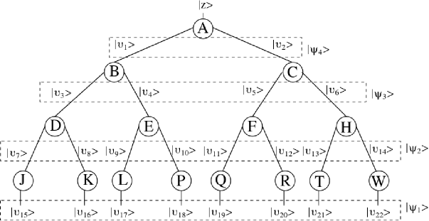
   Figure 4: Unsimplified BSQDD. Each layer corresponds to a set of gates which act on a specific qubit. For example, the gate $A$ acts on the most significant qubit while gates $J$ to $W$ act on the least significant qubit. The state ${\left|{\upsilon_{i}}\right\rangle}$ is the non normalized state obtained when a specific gate acts on a specific qubit. The state ${\left|{\psi_{i}}\right\rangle}$, as the sum of non normalized states, is the normalized state obtained after the gates of the layer $i$ act on qubit $i$. The state ${\left|{z}\right\rangle}$ is the basis state used for starting and state ${\left|{\psi_{1}}\right\rangle}$ is the desired quantum supposed state.

2. Reducing the BSQDD to obtain the final BSQDD. The goal is to have the lower bound on the number of quantum gates. To attempt this goal one needs to merge some nodes (gates) according to the links that can occur between qubits (like control qubit and target qubit). Fig. 5 shows BSQDDs with merged nodes (Fig. 5a and Fig. 5b) and the final BSQDD (Fig. 5c). The three BSQDDs in Fig. 5 are equivalent.

   

   (a) First merging nodes

   

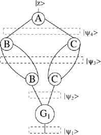
   (b) Second merging nodes

   

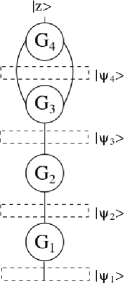
   (c) Final BSQDD

   Figure 5: The merging nodes to obtain the final BSQDD by using the following two rules: in two different branches of different nodes which correspond to the same next same node, the nodes merge; in different branches of different nodes which generate the same branch, the branches merge.

3. Converting the BSQDD to a quantum array which generates the desired quantum state (see Fig. 6).

   Figure 6: The quantum array generated by the final BSQDD. The array is obtained by adding the gates for the nodes in each layer of the final BSQDD. The starting point is the last layer and new gates are always placed to the right of gates that have already been placed in quantum array. Therefore the first gate is $G_{4}$, while the last is $G_{1}$.

Example 3.

Fig. 7 gives the three steps which allow to construct the state $\sqrt{\frac{1}{5}}({\left|{000}\right\rangle}+{\left|{010}\right\rangle}+{\left|{110}\right\rangle}+{\left|{001}\right\rangle}+{\left|{101}\right\rangle})$. The elementary gates used are respectively $\mathtt{R}(\theta)=\begin{pmatrix}\sqrt{\frac{3}{5}}&\sqrt{\frac{2}{5}}\\ \sqrt{\frac{2}{5}}&-\sqrt{\frac{3}{5}}\end{pmatrix}$, $\mathtt{R}(\alpha)=\begin{pmatrix}\sqrt{\frac{2}{3}}&\frac{1}{\sqrt{3}}\\ \frac{1}{\sqrt{3}}&-\sqrt{\frac{2}{3}}\end{pmatrix}$, the Hadamard gate $\mathtt{W}$ and the NOT gate $\mathtt{X}$. Then ${\left|{\psi_{3}}\right\rangle}=\sqrt{\frac{3}{5}}{\left|{000}\right\rangle}+\sqrt{\frac{2}{5}}{\left|{100}\right\rangle}$ and ${\left|{\psi_{2}}\right\rangle}=\sqrt{\frac{2}{5}}{\left|{000}\right\rangle}+\frac{1}{\sqrt{5}}{\left|{010}\right\rangle}+\frac{1}{\sqrt{5}}{\left|{100}\right\rangle}+\frac{1}{\sqrt{5}}{\left|{110}\right\rangle}$.

Fig. 8 presents the two first steps needed to compute the state used in example 1. The corresponding quantum array is the first dashed box of Fig. 10.

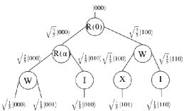
(a) Unsimplified BSQDD

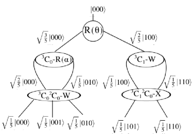
(b) Final BSQDD

(c) Corresponding quantum array

Figure 7: BSQDD to obtain state ${\left|{\psi_{1}}\right\rangle}=\sqrt{\frac{1}{5}}({\left|{000}\right\rangle}+{\left|{010}\right\rangle}+{\left|{110}\right\rangle}+{\left|{001}\right\rangle}+{\left|{101}\right\rangle})$.

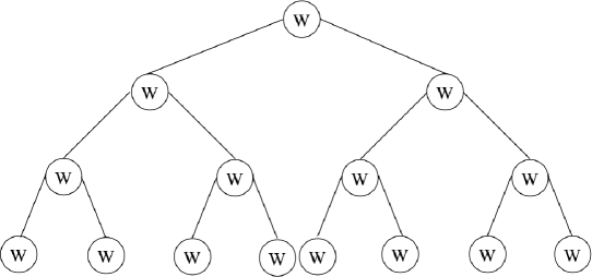
(a) Unsimplified BSQDD

(b) Final BSQDD

Figure 8: Two first steps needed to compute state used in example 1.

The process of retrieving data is done by the quantum NLSA which allows us to have the information we want after a measure on the flag qubit not on the first register. However, it can be useful to measure the register, especially in case of multi-values which satisfy $f(x)=1$. But, as it appears in the previous section, we will get each $2^{n}$ values with the same probability. In the method proposed by Rigui et al. [1] there are some ambiguities on how the system evolves and it is not clear on how a measure will give one of the sought patterns after the retrieving process.

The figure 9 summarizes our QAM-NLSA where it is possible to retrieve one of the sought states in multi-values retrieving scheme when a measure on the first register is done.

Figure 9: Schematic structure of QAM-NLSA. The $\mathtt{BDD}$ computes the learning process. The retrieving process is made by the gate $\mathtt{U}_{f}$ which marks the sought states, the gate $\mathtt{NLE}$ repeatedly computing the nonlinear evolution, the conditional gate $\mathtt{C}(\mathtt{BDD})^{{\dagger}}$ bringing back the first register to its initial state ${\left|{z}\right\rangle}$ and the conditional operator $\mathtt{CS}$ which maps the first register to the sought state ${\left|{x}\right\rangle}$.

1. The learning process is made by the operator $\mathtt{BDD}$.

2. The retrieving process is made by:

   1. The operator $\mathtt{NL}$ which marks the sought states with $\mathtt{U}_{f}$, computes repeatedly the nonlinear evolution $\mathtt{NLE}$ on the system and disentangles the first register from the flag qubit.

   2. The conditional operator $\mathtt{C}(\mathtt{BDD})^{{\dagger}}$ which acts on the first register and brings it back to its initial state ${\left|{z}\right\rangle}$ when the flag qubit is ${\left|{1}\right\rangle}$.

   3. The operator

      $$\mathtt{CS}=\mathbb{I}_{2^{n}}\otimes{\left|{0}\right\rangle}{\left\langle{0}\right|}+\left(\mathbb{I}_{2^{n}}-({\left|{z}\right\rangle}{\left\langle{z}\right|}+{\left|{x}\right\rangle}{\left\langle{x}\right|})+{\left|{x}\right\rangle}{\left\langle{z}\right|}+{\left|{z}\right\rangle}{\left\langle{x}\right|}\right)\otimes{\left|{1}\right\rangle}{\left\langle{1}\right|},$$ (20)

      which is a $(2^{n+1})\times(2^{n+1})$ conditional operator which maps the first register to the sought state ${\left|{x}\right\rangle}$ when the flag qubit is ${\left|{1}\right\rangle}$. Put differently,

      • if the flag qubit is ${\left|{0}\right\rangle}$ nothing is done;

      • if the flag qubit is ${\left|{1}\right\rangle}$ the $2^{n}\times 2^{n}$ operator

        $$\mathtt{S}=\mathbb{I}_{2^{n}}-({\left|{z}\right\rangle}{\left\langle{z}\right|}+{\left|{x}\right\rangle}{\left\langle{x}\right|})+{\left|{x}\right\rangle}{\left\langle{z}\right|}+{\left|{z}\right\rangle}{\left\langle{x}\right|}$$ (21)

        is applied on the first register.

      It is noteworthy that in the case of multi-patterns retrieving the sought state ${\left|{x}\right\rangle}$ can be a supposed state of all the sought states (for example ${\left|{x}\right\rangle}=\frac{1}{\sqrt{2}}({\left|{0010}\right\rangle}+{\left|{1010}\right\rangle})$ in the example 2).

   4. The system is observed by making a measurement on the first register and/or on the flag qubit to erase any ambiguity.

We also point out the fact that as the BSQDD method can compute any sought state, it can be useful to compute the operator $\mathtt{CS}$. Indeed, in the case of a complex sought state ${\left|{x}\right\rangle}$ where the Hadamard gates or other methods are inadequate, the BSQDD method can allow us to have the appropriate form of the operator $\mathtt{S}$.

Example 4.

The example 1 suggests the operator $\mathtt{S}=\mathbb{I}_{2}\otimes\mathbb{I}_{2}\otimes\mathtt{X}\otimes\mathbb{I}_{2}$. Therefore, the $\mathtt{CX}$ gate acts only on the second qubit, while the other qubits are unchanged. The figure 10 gives the evolution of the system.

}                      flag qubit

Figure 10: Schematic structure of QAM-NLSA of example 1. $\mathtt{W}$ is the Hadamard gate which puts (reverses to its initial state respectively) the first register in the superposed state before (after respectively) the $\mathtt{NL}$ computing the nonlinear algorithm acts. Note that states ${\left|{\psi}\right\rangle}$ and ${\left|{\Psi_{4}}\right\rangle}$ are those give by Eq. (17a) and Eq. (18h) respectively.

3.2 Analysis of the complexity of the nonlinear evolution algorithm

All the above description was made with the assumption that there is at most one value $x$ for which $f(x)=1$. Let us now consider the case where there can be more than one value satisfying $f(x)=1$. In the simple case where there are at most two values satisfying $f(x)=1$, the state (6) must be rewritten as

$${\left|{\Psi}\right\rangle}=\frac{1}{\sqrt{2^{n}}}[\sum_{\begin{subarray}{c}j_{n}j_{n-1}\ldots j_{1}=0\\ j_{n}j_{n-1}\ldots j_{2}\neq i_{n}i_{n-1}\ldots i_{2}\\ j_{n}j_{n-1}\ldots j_{2}\neq e_{n}e_{n-1}\ldots e_{2}\end{subarray}}^{1}{\left|{j_{n}j_{n-1}\ldots j_{1}}\right\rangle}{\left|{0}\right\rangle}+{\left|{i_{n}i_{n-1}\ldots(1-i_{1})}\right\rangle}{\left|{0}\right\rangle}+{\left|{i_{n}i_{n-1}\ldots i_{1}}\right\rangle}{\left|{1}\right\rangle}\\ +{\left|{e_{n}e_{n-1}\ldots(1-e_{1})}\right\rangle}{\left|{0}\right\rangle}+{\left|{e_{n}e_{n-1}\ldots e_{1}}\right\rangle}{\left|{1}\right\rangle}].$$ (22)

Highlighting the LSQ of the first register and the flag qubit, the second part of state (22) must be in one of the following states:

• if $i_{n}i_{n-1}\ldots i_{2}\neq e_{n}e_{n-1}\ldots e_{2}$,

  $${\left|{10}\right\rangle}+{\left|{01}\right\rangle}+{\left|{10}\right\rangle}+{\left|{01}\right\rangle},$$ (23a)

  $${\left|{10}\right\rangle}+{\left|{01}\right\rangle}+{\left|{00}\right\rangle}+{\left|{11}\right\rangle},$$ (23b)

  $${\left|{00}\right\rangle}+{\left|{11}\right\rangle}+{\left|{10}\right\rangle}+{\left|{01}\right\rangle},$$ (23c)

  $${\left|{00}\right\rangle}+{\left|{11}\right\rangle}+{\left|{00}\right\rangle}+{\left|{11}\right\rangle},$$ (23d)

• or if $i_{n}i_{n-1}\ldots i_{2}=e_{n}e_{n-1}\ldots e_{2}$,

  $${\left|{01}\right\rangle}+{\left|{11}\right\rangle},$$ (24)

  according to the fact that there is no repetition of value.

The action of the NLE gate on states (23) is the same as the one described in section 2. Taking a careful look on states (23), it seems that the NLE was already applied one time and this suggests that the NLE gate will be repeated $(n-1)$ times. The state (24) also supposes that the NLE gate was already applied thus the NLE gate will begin on the second LSQ and will be repeated $(n-1)$ times. Therefore, if there are at most two values $x$ for which $f(x)=1$, the number of steps of the QAM-NLSA is

$$\mathcal{O}(n-1),$$ (25a)

as the NLE gate starts on the second LSQ. It is easy to find that in the case where there are at most three values $$x f(x)=1$$ satisfying , when we start the repeated action of the NLE on the second LSQ of the first register, the number of steps of the QAM-NLSA is also

$$\mathcal{O}(n-1).$$ (25b)

According to the above observation, if there are at most $m$ values $x$ for which $f(x)=1$ and $r=\mathtt{int}(\log_{2}{m})$, that is the integer part of $\log_{2}{m}$, the NLE gate action starts on the $(r+1)^{th}$ LSQ of the first register and will be repeated $(n-r)$ times. Thus, the number of steps of the QAM-NLSA is

$$\mathcal{O}(n-r).$$ (26)

Example 5.

In order to enlighten the result (26), let us consider the parameters of example 1. The marked states are ${\left|{2}\right\rangle}={\left|{0010}\right\rangle}$, ${\left|{5}\right\rangle}={\left|{0101}\right\rangle}$, ${\left|{8}\right\rangle}={\left|{1000}\right\rangle}$, ${\left|{10}\right\rangle}={\left|{1010}\right\rangle}$, ${\left|{11}\right\rangle}={\left|{1011}\right\rangle}$, ${\left|{13}\right\rangle}={\left|{1101}\right\rangle}$ and ${\left|{15}\right\rangle}={\left|{1111}\right\rangle}$. The number of marked states is $m=7$ and $\log_{2}{m}=2.807$. Consequently, $r=2$; and the NLE gate action starts on the third LSQ of the register. Let us check that in detail. As in the example 1, we start with

$${\left|{\psi}\right\rangle}=\frac{1}{4}({\left|{0000}\right\rangle}+{\left|{0001}\right\rangle}+{\left|{0010}\right\rangle}+{\left|{0011}\right\rangle}+{\left|{0100}\right\rangle}+{\left|{0101}\right\rangle}+{\left|{0110}\right\rangle}+{\left|{0111}\right\rangle}\\ +{\left|{1000}\right\rangle}+{\left|{1001}\right\rangle}+{\left|{1010}\right\rangle}+{\left|{1011}\right\rangle}+{\left|{1100}\right\rangle}+{\left|{1101}\right\rangle}+{\left|{1110}\right\rangle}+{\left|{1111}\right\rangle}){\left|{0}\right\rangle}.$$ (27a)

The action of the oracle operator $$\mathtt{U}_{f}$$ yields

$${\left|{\Psi}\right\rangle}=\frac{1}{4}({\left|{0000}\right\rangle}{\left|{0}\right\rangle}+{\left|{0001}\right\rangle}{\left|{0}\right\rangle}+{\left|{0010}\right\rangle}{\left|{1}\right\rangle}+{\left|{0011}\right\rangle}{\left|{0}\right\rangle}+{\left|{0100}\right\rangle}{\left|{0}\right\rangle}+{\left|{0101}\right\rangle}{\left|{1}\right\rangle}+{\left|{0110}\right\rangle}{\left|{0}\right\rangle}\\ +{\left|{0111}\right\rangle}{\left|{0}\right\rangle}+{\left|{1000}\right\rangle}{\left|{1}\right\rangle}+{\left|{1001}\right\rangle}{\left|{0}\right\rangle}+{\left|{1010}\right\rangle}{\left|{1}\right\rangle}+{\left|{1011}\right\rangle}{\left|{1}\right\rangle}+{\left|{1100}\right\rangle}{\left|{0}\right\rangle}+{\left|{1101}\right\rangle}{\left|{1}\right\rangle}\\ +{\left|{1110}\right\rangle}{\left|{0}\right\rangle}+{\left|{1111}\right\rangle}{\left|{1}\right\rangle}).$$ (27b)

Finally, when taking a look on the MSQ, this is what we have:

$$\begin{split}{\left|{\Psi_{1}}\right\rangle}=\frac{1}{4}&({\left|{{\boxed{{\color[rgb]{0,0,1}0}}}000}\right\rangle}{\left|{{\boxed{{\color[rgb]{0,0,1}0}}}}\right\rangle}+{\left|{{\boxed{{\color[rgb]{0,0,1}1}}}000}\right\rangle}{\left|{{\boxed{{\color[rgb]{0,0,1}1}}}}\right\rangle}\\ &+{\left|{{\boxed{{\color[rgb]{0,0,1}0}}}001}\right\rangle}{\left|{{\boxed{{\color[rgb]{0,0,1}1}}}}\right\rangle}+{\left|{{\boxed{{\color[rgb]{0,0,1}1}}}001}\right\rangle}{\left|{{\boxed{{\color[rgb]{0,0,1}0}}}}\right\rangle}\\ &+{\left|{{\boxed{{\color[rgb]{0,0,1}0}}}010}\right\rangle}{\left|{{\boxed{{\color[rgb]{0,0,1}1}}}}\right\rangle}+{\left|{{\boxed{{\color[rgb]{0,0,1}1}}}010}\right\rangle}{\left|{{\boxed{{\color[rgb]{0,0,1}0}}}}\right\rangle}\\ &+{\left|{{\boxed{{\color[rgb]{0,0,1}0}}}011}\right\rangle}{\left|{{\boxed{{\color[rgb]{0,0,1}0}}}}\right\rangle}+{\left|{{\boxed{{\color[rgb]{0,0,1}1}}}011}\right\rangle}{\left|{{\boxed{{\color[rgb]{0,0,1}1}}}}\right\rangle}\\ &+{\left|{{\boxed{{\color[rgb]{0,0,1}0}}}100}\right\rangle}{\left|{{\boxed{{\color[rgb]{0,0,1}0}}}}\right\rangle}+{\left|{{\boxed{{\color[rgb]{0,0,1}1}}}100}\right\rangle}{\left|{{\boxed{{\color[rgb]{0,0,1}1}}}}\right\rangle}\\ &+{\left|{{\boxed{{\color[rgb]{0,0,1}0}}}101}\right\rangle}{\left|{{\boxed{{\color[rgb]{0,0,1}1}}}}\right\rangle}+{\left|{{\boxed{{\color[rgb]{0,0,1}1}}}101}\right\rangle}{\left|{{\boxed{{\color[rgb]{0,0,1}0}}}}\right\rangle}\\ &+{\left|{{\boxed{{\color[rgb]{0,0,1}0}}}110}\right\rangle}{\left|{{\boxed{{\color[rgb]{0,0,1}1}}}}\right\rangle}+{\left|{{\boxed{{\color[rgb]{0,0,1}1}}}110}\right\rangle}{\left|{{\boxed{{\color[rgb]{0,0,1}0}}}}\right\rangle}\\ &+{\left|{{\boxed{{\color[rgb]{0,0,1}0}}}111}\right\rangle}{\left|{{\boxed{{\color[rgb]{0,0,1}0}}}}\right\rangle}+{\left|{{\boxed{{\color[rgb]{0,0,1}1}}}111}\right\rangle}{\left|{{\boxed{{\color[rgb]{0,0,1}1}}}}\right\rangle})\end{split}$$ (28c)

and applying the NLE gate the last time produces

$$\begin{split}{\left|{\Psi_{2}}\right\rangle}=\frac{1}{4}&({\left|{{\boxed{{\color[rgb]{0,0,1}0}}}000}\right\rangle}+{\left|{{\boxed{{\color[rgb]{0,0,1}1}}}000}\right\rangle}\\ &+{\left|{{\boxed{{\color[rgb]{0,0,1}0}}}001}\right\rangle}+{\left|{{\boxed{{\color[rgb]{0,0,1}1}}}001}\right\rangle}\\ &+{\left|{{\boxed{{\color[rgb]{0,0,1}0}}}010}\right\rangle}+{\left|{{\boxed{{\color[rgb]{0,0,1}1}}}010}\right\rangle}\\ &+{\left|{{\boxed{{\color[rgb]{0,0,1}0}}}011}\right\rangle}+{\left|{{\boxed{{\color[rgb]{0,0,1}1}}}011}\right\rangle}\\ &+{\left|{{\boxed{{\color[rgb]{0,0,1}0}}}100}\right\rangle}+{\left|{{\boxed{{\color[rgb]{0,0,1}1}}}100}\right\rangle}\\ &+{\left|{{\boxed{{\color[rgb]{0,0,1}0}}}101}\right\rangle}+{\left|{{\boxed{{\color[rgb]{0,0,1}1}}}101}\right\rangle}\\ &+{\left|{{\boxed{{\color[rgb]{0,0,1}0}}}110}\right\rangle}+{\left|{{\boxed{{\color[rgb]{0,0,1}1}}}110}\right\rangle}\\ &+{\left|{{\boxed{{\color[rgb]{0,0,1}0}}}111}\right\rangle}+{\left|{{\boxed{{\color[rgb]{0,0,1}1}}}111}\right\rangle}){\left|{{\boxed{{\color[rgb]{0,0,1}1}}}}\right\rangle}\end{split}$$ (28d)

It effectively appears that the NLE gate was repeated $(n-r)=4-2=2$ times.

If the values of $t$ qubits of our first register are known (i.e., $t$ qubits have been measured or are already disentangled to others, or the oracle acts on a subspace of $(n-t)$ qubits) and there is at most $m$ values $x$ for which $f(x)=1$, the NLE gate will act repeatedly $((n-t)-r)$ times that starts on the $(r+1)^{th}$ LSQ. As the $t$ qubits which are already known will be ignored, it is clear that $m\leq 2^{n-t}$. Consequently, the number of steps of the QAM-NLSA is

$$\mathcal{O}((n-t)-r).$$ (29)

Now, if in the first register which is an $n$-qubit system, the computed patterns are $p\leq 2^{n}$ and we stated $b=\mathtt{ceil}(\log_{2}{p})$, i.e. the least integer greater or equal to $\log_{2}{p}$, $m$ the number of value $x$ for which $f(x)=1$. The NLE gate will act repeatedly $(b-r)$ times. Therefore, the number of steps of the QAM-NLSA is

$$\mathcal{O}(b-r)$$ (30)

for which the upper bound is the Eq.(26). Note that the starting point of the NLE gate action will always be the $(r+1)^{th}$ LSQ.

If we know the values of $t$ qubits of our first register, it supposes that we must view the system in terms of $q\leq p\leq 2^{n}$ patterns; consequently the number of values $m$ for which $f(x)=1$ is $m\leq q$. For $c=\mathtt{ceil}(\log_{2}{q})$, the NLE gate will act repeatedly $(c-r)$ times. Therefore, the number of steps of the QAM-NLSA takes the general form

$$\mathcal{O}(c-r).$$ (31)

Example 6.

• If we consider again the parameters of the example 1, we find that $p=16$, the number of known qubits is $t=0$. Consequently $q=p=16$, and $\log_{2}{q}=\log_{2}{16}=4.0$, thus $c=4$, $m=1$ and $r=0$. The NLE gate will act repeatedly, $(c-r)=4-0=4$ times.

• In the example 2, $t=1$. Consequently $q=8$ according to the assumption taken in this example. $\log_{2}{q}=\log_{2}{8}=3.0$, thus $c=3$. $m=1$, then $r=0$. The NLE gate will act repeatedly, $(c-r)=3-0=3$ times.

• In the example 5, $t=0$ and $q=16$ but $m=7$. Then $\log_{2}{m}=2.807$. That is $r=2$. The NLE gate will act repeatedly $(c-r)=4-2=2$ times.

It is noteworthy that when the state ${\left|{01}\right\rangle}+{\left|{11}\right\rangle}$ appears the last time, the NLE gate acts repeatedly. The state ${\left|{01}\right\rangle}+{\left|{11}\right\rangle}$ then does not evolve. Its nonlinear evolution must be like that of the state (8a). Such a nonlinear evolution of the state ${\left|{01}\right\rangle}+{\left|{11}\right\rangle}$ is described as follows:

• Apply operator $\mathtt{U}$:

  $$\mathtt{U}({\left|{01}\right\rangle}+{\left|{11}\right\rangle})=\frac{1}{\sqrt{2}}({\left|{00}\right\rangle}+{\left|{01}\right\rangle}+{\left|{10}\right\rangle}-{\left|{11}\right\rangle}).$$ (32)

• Apply the nonlinear operator $\mathtt{NL}^{-}$:

  $$\mathtt{NL}^{-}[\frac{1}{\sqrt{2}}({\left|{00}\right\rangle}+{\left|{01}\right\rangle}+{\left|{10}\right\rangle}-{\left|{11}\right\rangle})]=\sqrt{2}{\left|{0}\right\rangle}(\delta{\left|{0}\right\rangle}+\epsilon{\left|{1}\right\rangle}),$$ (33)

  where $\delta,\epsilon\in\mathbb{C},\,|\delta|^{2}+|\epsilon|^{2}=1$. As we see on the state (33), the action of the nonlinear operator $\mathtt{NL}^{-}$ is also not specified like on the state (11a).

• Apply the second nonlinear operator $\mathtt{NL}^{+}$:

  $$\mathtt{NL}^{+}[\sqrt{2}{\left|{0}\right\rangle}(\delta{\left|{0}\right\rangle}+\epsilon{\left|{1}\right\rangle})]=\sqrt{2}{\left|{00}\right\rangle}.$$ (34)

  The general form of the unitary matrix $\mathtt{NL}^{+}$ which maps the generic 1-qubit $\delta{\left|{0}\right\rangle}+\epsilon{\left|{1}\right\rangle}$ to ${\left|{0}\right\rangle}$ is

  $$\mathtt{\Pi}=\begin{pmatrix}\delta^{\ast}&\epsilon^{\ast}\\ \mp\gamma\epsilon&\pm\gamma\delta\end{pmatrix},\,\,\gamma=\pm i\text{ or }\pm 1\;(i^{2}=-1),$$ (35)

  where $\,\delta,\,\epsilon\in\mathbb{C},\,|\delta|^{2}+|\epsilon|^{2}=1$.

• Apply the NOT gate $\mathtt{X}$ on the flag qubit and the Hadamard gate $\mathtt{W}$ on the first qubit.

We summarize below this nonlinear evolution of state ${\left|{01}\right\rangle}+{\left|{11}\right\rangle}$ and give its corresponding circuit (see Fig. 11)

$${\left|{01}\right\rangle}+{\left|{11}\right\rangle}\xrightarrow{\mathtt{U}}\frac{1}{\sqrt{2}}({\left|{00}\right\rangle}+{\left|{01}\right\rangle}+{\left|{10}\right\rangle}-{\left|{11}\right\rangle})\xrightarrow{\mathtt{NL}^{-}}\sqrt{2}{\left|{0}\right\rangle}(\delta{\left|{0}\right\rangle}+\epsilon{\left|{1}\right\rangle})\xrightarrow{\mathtt{NL}^{+}}\sqrt{2}{\left|{00}\right\rangle}\xrightarrow{\mathtt{W}\otimes\mathtt{X}}{\left|{01}\right\rangle}+{\left|{11}\right\rangle}.$$ (36)

Figure 11: Equivalent circuit of the nonlinear evolution (36).

Algorithm 2 Algorithm of QAM-NLSA

1:  Store patterns using the operator $\mathtt{BDD}$ and put the flag qubit to ${\left|{0}\right\rangle}$

2:  Apply the oracle $\mathtt{U}_{f}$

3:  repeat $(c-r)$ times step (4) to step (6) (i.e., one time per qubit of the first register starting from $(r+1)^{th}$ qubit with the flag qubit)

4:      Apply the unitary operator $\mathtt{U}$

5:  

1. Apply the nonlinear operator $\mathtt{NL}^{-}$

2. Apply the nonlinear operator $\mathtt{NL}^{+}$

6:      Apply the Hadamard operator $\mathtt{W}$ on the qubit of the first register and the NOT operator $\mathtt{X}$ on the flag qubit

7:  Observe the flag qubit

8:  if the flag qubit is in state ${\left|{0}\right\rangle}$

9:      Conclude

10:  else 1. Apply the conditional operator $\mathtt{C}(\mathtt{BDD})^{{\dagger}}$ to kick back the first register to its initial state 2. Apply the conditional operator $\mathtt{CS}$ to flip the register to the sought state 3. Observe the first register

Finally, the Algorithm (2) can describe the QAM-NLSA where

• $n$ is the number of qubit of the first register,

• $p\leq 2^{n}$ the number of stored patterns,

• $q\leq p$ the number of stored patterns if the values of $t$ qubits are known (i.e. $t$ qubits have been measured or are already disentangled to others or the oracle acts on a subspace of $(n-t)$ qubits),

• $c=\mathtt{ceil}(\log_{2}{q})$, i.e. the least integer greater or equal to $\log_{2}{q}$,

• $m\leq q$ the number of values $x$ for which $f(x)=1$,

• $r=\mathtt{int}(\log_{2}{m})$ is the integer part of $\log_{2}{m}$.

Remark 1.

The goal of the NLA is to determine if a needed state exist in a register. The conditional gates are made to act only if this state exists in the register. Therefore gate $mathtt{S}$ can only computes memorised states even in case of completion problem.

4 Taking into account the quantum noise

We will briefly analyze in this section how our QAM-NLSA evolves in the presence of quantum noise. As the NLSA evolves qubit per qubit, we will consider only the single qubit quantum noise channels as described in [12, 13]. The quantum states to be considered will be the density operators instead of state vectors.

4.1 Single qubit quantum noise channels

If $\rho_{in}={\left|{\psi}\right\rangle}{\left\langle{\psi}\right|}$ is the density matrix of the state ${\left|{\psi}\right\rangle}$, the effect of the environment leads in the Kraus representation to

$$\rho_{out}=\mathcal{K}(\rho_{in})=\sum_{i}E_{i}\rho_{in}E^{{\dagger}}_{i},\,\,\sum_{i}E^{{\dagger}}_{i}E_{i}=\mathbb{I},$$ (37)

where $E_{i}$ are the errors operators or Kraus operators which completely describe here the single qubit quantum noise channels briefly presented in the Table 1.

Noisy channels	Description	Set of Kraus operators $\{E_{i}\}$
Bit flip	Induced by dissipation, it flips the state ${\left|{k}\right\rangle}$ to ${\left|{\bar{k}}\right\rangle},\,k=0,1$.	$\{\sqrt{1-\eta}\mathtt{X}^{0},\sqrt{\eta}\mathtt{X}\}$
Phase flip	Induced by decoherence, it flips the state ${\left|{k}\right\rangle}$ to $(-1)^{k}{\left|{k}\right\rangle},\,k=0,1$.	$\{\sqrt{1-\eta}\mathtt{Z}^{0},\sqrt{\eta}\mathtt{Z}\}$
Bit-phase flip	It is a joint action of bit and phase flips.	$\{\sqrt{1-\eta}\mathtt{Y}^{0},\sqrt{\eta}\mathtt{Y}\}$
Amplitude damping	It transforms state ${\left|{1}\right\rangle}$ into state ${\left|{0}\right\rangle}$ but leaves state ${\left|{0}\right\rangle}$ unchanged. It should be viewed as energy dissipation.	$\{{\left|{0}\right\rangle}{\left\langle{0}\right|}+\sqrt{1-\eta}{\left|{1}\right\rangle}{\left\langle{1}\right|},\sqrt{\eta}{\left|{0}\right\rangle}{\left\langle{1}\right|}\}$
Phase damping	It involves the loss of information about relatives phases in quantum state	$\{{\left|{0}\right\rangle}{\left\langle{0}\right|}+\sqrt{1-\eta}{\left|{1}\right\rangle}{\left\langle{1}\right|},\sqrt{\eta}{\left|{1}\right\rangle}{\left\langle{1}\right|}\}$
Depolarizing channel	It transforms any state into a completed mixed state.	$\{\sqrt{1-\eta}\mathbb{I},\sqrt{\frac{\eta}{3}}\mathtt{X},\sqrt{\frac{\eta}{3}}\mathtt{Y},\sqrt{\frac{\eta}{3}}\mathtt{Z}\}$

Table 1: Single qubit quantum noise channels. $\mathtt{X}_{i=0,1,2,3}=\mathbb{I},\,\mathtt{X},\,\mathtt{Y},\,\mathtt{Z}$ are Pauli matrices and $\eta\in[0,1]$ is the probability of a state to be affected by the noise. It should be noted that $\mathtt{X}_{i=1,2,3}^{0}=\mathbb{I}$ is not an error operator. Therefore, value $1-\eta$ associated to this operator represents the probability that no error occurs.

4.2 Quantum associative memories with noise - bit flip model

We suppose that during the nonlinear evolution (NLE), step 4 to step 6 of the Algorithm 1, the quantum noise occurs with the probability $\eta\in[0,1]$ after the action of each gate of the $\mathtt{NLE}$ gate. We assume that

• each gate operates before the error proceeds and it is the same error,

• the first register is an $n$-qubit system and that the probability $\eta$ of a state to be affected by the noise is independent of the total number of network qubits,

• errors are located at each time step in the network affecting ${\left|{\ell}\right\rangle}$ and ${\left|{k}\right\rangle}$.

Figure 12: Schematic structure of the NLSA with quantum noise.

Now, we analyse the effect of each quantum noise channels during evolution of states (6). Thus, while we reduce the system to the two qubits ${\left|{\ell}\right\rangle}$ and ${\left|{k}\right\rangle}$ we have

$$\rho_{out}=\sum_{i}E_{i}\left(\mathtt{W}\otimes\mathtt{X}\left[\sum_{i}E_{i}\left(\mathtt{NL}^{+}\left[\sum_{i}E_{i}\left(\mathtt{NL}^{-}\left[\sum_{i}E_{i}\left(\mathtt{U}\rho_{in}\mathtt{U}^{\dagger}\right)E_{i}^{\dagger}\right](\mathtt{NL}^{-})^{\dagger}\right)E_{i}^{\dagger}\right](\mathtt{NL}^{+})^{\dagger}\right)E_{i}^{\dagger}\right]\mathtt{W}^{\dagger}\otimes\mathtt{X}^{\dagger}\right)E_{i}^{\dagger}.$$ (38)

Because for each step of NLE, we look a two qubits system, then errors operators to apply will be a tensor product of operators of single quantum noise models.

For the bit flip model, the set of operators where $r$ index the qubit of first register and $f$ index the flag qubit is given below by the tensor product $\{\mathbb{I}_{r},\mathtt{X}_{r}\}\otimes\{\mathbb{I}_{f},\mathtt{X}_{f}\}$:

$$\begin{split}E_{1}&=\sqrt{1-\eta_{r}}\sqrt{1-\eta_{f}}\mathbb{I}_{r}\otimes\mathbb{I}_{f}\\ E_{2}&=\sqrt{1-\eta_{r}}\sqrt{\eta_{f}}\mathbb{I}_{r}\otimes\mathtt{X}_{f}\\ E_{3}&=\sqrt{\eta_{r}}\sqrt{1-\eta_{f}}\mathtt{X}_{r}\otimes\mathbb{I}_{f}\\ E_{4}&=\sqrt{\eta_{r}}\sqrt{\eta_{f}}\mathtt{X}_{r}\otimes\mathtt{X}_{f}.\end{split}$$ (39)

Remark that according to equation (38), $\rho_{out}$ is the sum of $256$ matrix for bit flip model.

Due to entanglement the system must be observed completely. So, without the normalization constant, the input matrix is

$$\begin{split}\rho_{in}&={\left|{\psi}\right\rangle}{\left\langle{\psi}\right|}\\ &=\left[\sum_{\begin{subarray}{c}j_{n}j_{n-1}\ldots j_{2}=0\\ j_{n}j_{n-1}\ldots j_{2}\neq i_{n}i_{n-1}\ldots i_{2}\end{subarray}}^{1}{\left|{j_{n}j_{n-1}\ldots j_{2}0}\right\rangle}{\left|{0}\right\rangle}+{\left|{j_{n}j_{n-1}\ldots j_{2}1}\right\rangle}{\left|{0}\right\rangle}+{\left|{i_{n}i_{n-1}\ldots(1-i_{1})}\right\rangle}{\left|{0}\right\rangle}+{\left|{i_{n}i_{n-1}\ldots i_{1}}\right\rangle}{\left|{1}\right\rangle}\right]\\ &\left[\sum_{\begin{subarray}{c}j_{n}j_{n-1}\ldots j_{2}=0\\ j_{n}j_{n-1}\ldots j_{2}\neq i_{n}i_{n-1}\ldots i_{2}\end{subarray}}^{1}{\left\langle{j_{n}j_{n-1}\ldots j_{2}0}\right|}{\left\langle{0}\right|}+{\left\langle{j_{n}j_{n-1}\ldots j_{2}1}\right|}{\left\langle{0}\right|}+{\left\langle{i_{n}i_{n-1}\ldots(1-i_{1})}\right|}{\left\langle{0}\right|}+{\left\langle{i_{n}i_{n-1}\ldots i_{1}}\right|}{\left\langle{1}\right|}\right],\end{split}$$ (40)

while the sought output density matrix is

$$\Omega=\left(\left[\sum_{j_{n}j_{n-1}\ldots j_{1}=0}^{1}{\left|{j_{n}j_{n-1}\ldots j_{1}}\right\rangle}\right]\left[\sum_{j_{n}j_{n-1}\ldots j_{1}=0}^{1}{\left\langle{j_{n}j_{n-1}\ldots j_{1}}\right|}\right]\right)\otimes{\left|{1}\right\rangle}{\left\langle{1}\right|}.$$ (41)

To evaluate the influence of the quantum noise on the effectiveness of the algorithm, we will compute the fidelity between the sought output and the obtained output. Let $\sigma$ be the density matrix of the sought output. The fidelity then is

$$\mathcal{F}_{1}(\sigma,\Gamma)=tr\sqrt{\sqrt{\sigma}\Gamma\sqrt{\sigma}},$$ (42)

with $0\leq\mathcal{F}_{1}(\sigma,\Gamma)\leq 1$. $\mathcal{F}_{1}(\sigma,\Gamma)=0$ if $\sigma$ and $\Gamma$ are orthogonal and $\mathcal{F}_{1}(\sigma,\Gamma)=1$ if $\sigma=\Gamma$.

If we only focus on the effectiveness of the quantum noise on the NLE, that is before the retrieving process, we can consider that the sought output is a pure state ${\left|{\psi}\right\rangle}=\sum_{x}{\left|{x}\right\rangle}={\left|{\phi_{1}}\right\rangle}\otimes{\left|{\phi_{2}}\right\rangle}\dots\otimes{\left|{\phi_{n}}\right\rangle},\,{\left|{\phi_{j}}\right\rangle}=\alpha_{j}{\left|{0}\right\rangle}+\beta_{j}{\left|{1}\right\rangle}$ ($|\alpha_{j}|^{2}+|\beta_{j}|^{2}=1$), and then the equation (42) can be written as

$$\mathcal{F}_{0}({\left|{\psi}\right\rangle},\rho_{out})=\sqrt{{\left\langle{\psi}\right|}\rho_{out}{\left|{\psi}\right\rangle}}.$$ (43)

4.3 Simulation

We suppose that

$$\begin{split}\mathtt{NL}^{-}&=\mathtt{CX}^{1}_{fr}\mathtt{CW}^{0}_{rf}\mathtt{CW}^{1}_{rf}\\ &=\frac{1}{\sqrt{2}}\begin{pmatrix}1&1&0&0\\ 0&0&1&-1\\ 0&0&1&1\\ 1&-1&0&0\end{pmatrix},\end{split}$$ (44)

and according to equations (44), we can choose $\mathtt{M}=\mathtt{W}$. We also consider that $\eta_{r}=\eta_{f}=\epsilon$, according to the fact the error operator is applied on states ${\left|{\ell}\right\rangle}$ and ${\left|{k}\right\rangle}$ simultaneously (i.e., error arises on this qubits at the same time), thus we can consider that the probability of error is identical for both qubits. The set of operators is now

$$\begin{split}E_{1}&=(1-\epsilon)\mathbb{I}_{r}\otimes\mathbb{I}_{f}\\ E_{2}&=\sqrt{\epsilon(1-\epsilon)}\mathbb{I}_{r}\otimes\mathtt{X}_{f}\\ E_{3}&=\sqrt{\epsilon(1-\epsilon)}\mathtt{X}_{r}\otimes\mathbb{I}_{f}\\ E_{4}&=\epsilon\mathtt{X}_{r}\otimes\mathtt{X}_{f}.\end{split}$$ (45)

Because it is the flag qubit which is observed, we only extract its density matrix $\rho_{out}$ to evaluate fidelity.

4.3.1 Case where the sought state does not exist in the first register

Here the sought output of the flag qubit is ${\left|{0}\right\rangle}$.

If the first register has $$n$$ qubits,

$$\rho_{out}=\begin{pmatrix}1+\frac{1}{2}[(1-2\epsilon)^{3n}-1]&0\\ 0&-\frac{1}{2}[(1-2\epsilon)^{3n}-1]\end{pmatrix},$$ (46a)

then

$$\mathcal{F}_{0}({\left|{0}\right\rangle},\rho_{out})=\sqrt{1+\frac{1}{2}[(1-2\epsilon)^{3n}-1]}.$$ (46b)

Indeed,

• if the first register has only one qubit,

  $$\rho_{out}=\begin{pmatrix}1+\frac{1}{2}[(1-2\epsilon)^{3}-1]&0\\ 0&-\frac{1}{2}[(1-2\epsilon)^{3}-1]\end{pmatrix};$$ (47)

• if the first register has three qubits,

  $$\rho_{out}=\begin{pmatrix}1+\frac{1}{2}[(1-2\epsilon)^{9}-1]&0\\ 0&-\frac{1}{2}[(1-2\epsilon)^{9}-1]\end{pmatrix}.$$ (48)

As we shall see on Fig. 13 and according to equation (46b), while $\epsilon<0.5$ the fidelity is upper than $0.7$. But it decreases for $\epsilon\geq 0.5$ if the $n$ is an odd number, and increases if $n$ is an even one. For $n$ as an odd number (see Fig. 13a, one qubit), the area between $0.4$ and $0.6$ can be viewed as a stability area, i.e., the area where fidelity is maintained around $0.7$. For $n$ as an even number (see Fig. 13b, six qubits), this stability area grows with the number of qubit. Therefore, if the sought state does not exist in the first register, the QAM-NLSA is more resistant to noise when the register has an even number of qubit.

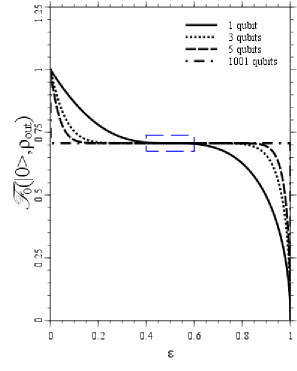
(a) If $n$ is odd

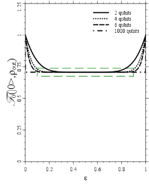
(b) If $n$ is even

Figure 13: Evolution of the fidelity $\mathcal{F}_{0}({\left|{0}\right\rangle},\rho_{out})$ at the end of NLE steps, in the case where the sought state does not exist in the first register, (a) for $1$, $3$, $5$ and $1001$ qubits and (b) for $2$, $4$, $6$ and $1000$ qubits. The dashed blue and green rectangles enlighten the stability area.

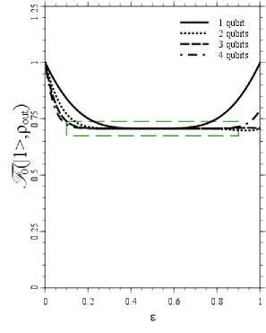
Figure 14: Evolution of the fidelity $\mathcal{F}_{0}({\left|{1}\right\rangle},\rho_{out})$ at the end of NLE steps for $1$, $2$, $3$ and $4$ qubits in the case where the sought state exists in the first register.

4.3.2 Case where the sought state exists in the first register

Here the sought output of the flag qubit is ${\left|{1}\right\rangle}$.

If the first register has $$n n>1$$ () qubits

$$\rho_{out}=\begin{pmatrix}-\frac{1}{2}\frac{f(\epsilon^{4n})}{2^{2n-3}}&0\\ 0&1+\frac{1}{2}\frac{f(\epsilon^{4n})}{2^{2n-3}}\end{pmatrix},$$ (49a)

where $$f \epsilon^{4n}$$ is a polynomial function which grows with . Then,

$$\mathcal{F}_{0}({\left|{1}\right\rangle},\rho_{out})=\sqrt{1+\frac{1}{2}[(1-2\epsilon)^{4}-1]},\text{ for }n=1,$$ (49b)

or

$$\mathcal{F}_{0}({\left|{1}\right\rangle},\rho_{out})=\sqrt{1+\frac{1}{2}\frac{f(\epsilon^{4n})}{2^{2n-3}}}\text{ for }n>1.$$ (49c)

Indeed,

• if the first register has only one qubit,

  $$\rho_{out}=\begin{pmatrix}-\frac{1}{2}[(1-2\epsilon)^{4}-1]&0\\ 0&1+\frac{1}{2}[(1-2\epsilon)^{4}-1]\end{pmatrix};$$ (50)

• if the first register has two qubits,

  $$\rho_{out}=\begin{pmatrix}-\frac{\frac{1}{2}[((1-2\epsilon)^{8}-1)+((1-2\epsilon)^{7}-1)]}{2}&0\\ 0&1+\frac{\frac{1}{2}[((1-2\epsilon)^{8}-1)+((1-2\epsilon)^{7}-1)]}{2}\end{pmatrix};$$ (51)

• if the first register has four qubits,

  $$\begin{pmatrix}-\frac{\frac{1}{2}\begin{bmatrix}((1-2\epsilon)^{16}-1)+5((1-2\epsilon)^{15}-1)\\ +15((1-2\epsilon)^{14}-1)+13((1-2\epsilon)^{13}-1)\\ +0((1-2\epsilon)^{12}-1)-6((1-2\epsilon)^{11}-1)\\ +5((1-2\epsilon)^{10}-1)-((1-2\epsilon)^{9}-1)\\ -((1-2\epsilon)^{8}-1)+((1-2\epsilon)^{7}-1)\end{bmatrix}}{2^{5}}&0\\ 0&1+\frac{\frac{1}{2}\begin{bmatrix}((1-2\epsilon)^{16}-1)+5((1-2\epsilon)^{15}-1)\\ +15((1-2\epsilon)^{14}-1)+13((1-2\epsilon)^{13}-1)\\ +0((1-2\epsilon)^{12}-1)-6((1-2\epsilon)^{11}-1)\\ +5((1-2\epsilon)^{10}-1)-((1-2\epsilon)^{9}-1)\\ -((1-2\epsilon)^{8}-1)+((1-2\epsilon)^{7}-1)\end{bmatrix}}{2^{5}}\end{pmatrix}.$$ (52)

As we see on Fig. 14 and according to equation (49c), whatever the value of $\epsilon$ the fidelity is greater than $0.7$. In other words, if the sought state exists in the first register, the QAM-NLSA is resistant to noise whatever the number of qubit. We also see that the stability area enlightened by the dashed green rectangle on Fig. 14 grows with the number of qubit. That stability area is the same as those shown on Fig. 13.

From the above simulations, it appears that QAM-NLSA is affected by the noise during its implementation. In the particular case of bit flip channel, the fidelity between the unaffected and affected systems is about $70\%$ and this value does not change even if the number of qubit in the first register grows.

5 Conclusion

We have proposed a model of the QAM-NLSA similar to that of Rigui et al. [1]. However, the model we propose differs with the possibility to retrieve one of the sought states in multi-values retrieving when a measure on the first register is done.

Firstly, we have described the NLSA put forth by Abrams and Lloyd in [3] with notations that overcome some ambiguities due to the notations of Rigui et al. and Czachor [7] and by summarizing each step of the nonlinear evolution with an equivalent circuit. A good general form of the unitary matrix $\mathtt{NL}^{+}$ which acts on the generic flag qubit $\alpha{\left|{0}\right\rangle}+\beta{\left|{1}\right\rangle}$ was given thereby correcting the wrong one given by Rigui et al. . Secondly, we have described our model of the Quantum Associative Neural Network where we have introduced a $(2^{n+1})\times(2^{n+1})$ conditional operator $\mathtt{CS}$ which maps the first register to the sought state ${\left|{x}\right\rangle}$ when the flag qubit is ${\left|{1}\right\rangle}$, where $n$ is the number of qubit of the first register. If $n$ is the number of qubit of the first register, $p\leq 2^{n}$ the number of stored patterns, $q\leq p$ the number of stored patterns if the values of $t$ qubits are known (i.e., $t$ qubits have been measured or have already been disentangled to others or the oracle acts on a subspace of $(n-t)$ qubits), $m\leq q$ the number of values $x$ for which $f(x)=1$, $c=\mathtt{ceil}(\log_{2}{q})$ the least integer greater or equal to $\log_{2}{q}$, and $r=\mathtt{int}(\log_{2}{m})$ the integer part of $\log_{2}{m}$, then the time complexity of our algorithm is $\mathcal{O}(c-r)$. It is better than Grover’s algorithm and its modified forms which need $\mathcal{O}(\sqrt{\frac{2^{n}}{m}})$ steps when they are used as the retrieval algorithm. An example to illustrate the results given by our analysis was done. It is noteworthy that our algorithm also allows to measure the flag qubit to erase any ambiguity on the result given by a measurement on the first register. This possibility is introduce by the use of two conditional gates who do not affect the flag qubit after nonlinear evolution.

Finally, we have briefly analysed the influence of the quantum noise namely bit flip channel on our model of the QAM-NLSA. We found that the bit flip channel leaves the QAM unaffected fully at $70\%$ if the sought state is present in the first register or if the register has an even number of qubit when the sought state does not exist. However, when the first register has an odd number of qubit and the sought state does not exist, the bit flip channel is extremely destructive when the probability $\epsilon>0.5$.

Further work will be undertaken in order study in details the influence of quantum noise related to the quantum network construction through errors characterizing the qubit time evolution and gate application in both the first register and the flag qubit.

6 Acknowledgments

Authors are very grateful to Dr D.E. Houpa Danga for useful discussions and remarks. We are thankful to M. A.L. Kamga for proofreading the work.

References

- [1] Rigui Zhou, Huian Wang, Qian Wu, and Yang Shi. Quantum Associative Neural Network with Nonlinear Search Algorithm. International Journal of Theoretical Physics, 51(3):705–723, March 2012.
- [2] David Rosenbaum. Binary superposed quantum decision diagrams. Quantum Information Processing, 9(4):463–496, August 2010.
- [3] Daniel S. Abrams and Seth Lloyd. Nonlinear Quantum Mechanics Implies Polynomial-Time Solution for -Complete and # Problems. Phys. Rev. Lett., 81:3992–3995, Nov 1998.
- [4] D. Ventura and T.R. Martinez. Quantum Associative Memory. Inf. Sci. Inf. Comput. Sci., 124(1-4):273–296, 2000.
- [5] A. A. Ezhov, A. V. Nifanova, and Dan Ventura. Quantum associative memory with distributed queries. Inf. Sci. Inf. Comput. Sci., 128(3-4):271–293, October 2000.
- [6] J.-P. Tchapet Njafa, S.G. Nana Engo, and Paul Woafo. Quantum Associative Memory with Improved Distributed Queries. International Journal of Theoretical Physics, 52(6):1787–1801, June 2013.
- [7] Marek Czachor. Notes on nonlinear quantum algorithms. Acta Phys. Slov., 48:157, feb 1998.
- [8] Joseph Polchinski. Weisberg’s Nonlinear Quantum Mechanics and the Einstein-Podolsky-Rosen Paradox. Physical Review Letters. Volume 66, Number 4, 1991.
- [9] David A Meyer and Thomas G Wong. Nonlinear quantum search using the Gross–Pitaevskii equation. New Journal of Physics, 15(6):063014, 2013.
- [10] P. J. Salas. Noise effect on Grover algorithm. The European Physical Journal D, 46(2):365–373, February 2008.
- [11] Piotr Gawron, Jerzy Klamka, and Ryszard Winiarczyk. Noise effects in the quantum search algorithm from the viewpoint of computational complexity. Applied Mathematics and Computer Science, 22(2):493–499, 2012.
- [12] Michael A. Nielsen and Isaac L. Chuang. Quantum Computation and Quantum Information (Cambridge Series on Information and the Natural Sciences). Cambridge University Press, New York, NY, USA, 10 edition, January 2000.
- [13] Colin P. Williams and Scott H. Clearwater. Explorations in Quantum Computing. Springer-Verlag TELOS, Santa Clara, CA, USA, 1998.