2 The Feynman path integral
Consider the Euclidean time Lagrangian with acceleration given by
ℒ = − γ 2 ( d 2 x d t 2 ) 2 − α 2 ( d x d t ) 2 − Φ ( x ) ℒ 𝛾 2 superscript superscript 𝑑 2 𝑥 𝑑 superscript 𝑡 2 2 𝛼 2 superscript 𝑑 𝑥 𝑑 𝑡 2 Φ 𝑥 \mathcal{L}=-\frac{\gamma}{2}(\frac{d^{2}x}{dt^{2}})^{2}-\frac{\alpha}{2}(\frac{dx}{dt})^{2}-\Phi(x) (2)
with the acceleration action for finite Euclidean time τ 𝜏 \tau
𝒮 [ x ] = ∫ 0 τ 𝑑 t ℒ 𝒮 delimited-[] 𝑥 superscript subscript 0 𝜏 differential-d 𝑡 ℒ \mathcal{S}[x]=\int_{0}^{\tau}dt\mathcal{L} (3)
The Feynman path integral for finite Euclidean time is given by
𝒦 ( x f , x ˙ f ; x i , x ˙ i ) = ∫ D X e 𝒮 [ x ] | ( x i , x ˙ i ; x f , x ˙ f ) 𝒦 subscript 𝑥 𝑓 subscript ˙ 𝑥 𝑓 subscript 𝑥 𝑖 subscript ˙ 𝑥 𝑖 evaluated-at 𝐷 𝑋 superscript 𝑒 𝒮 delimited-[] 𝑥 subscript 𝑥 𝑖 subscript ˙ 𝑥 𝑖 subscript 𝑥 𝑓 subscript ˙ 𝑥 𝑓 \displaystyle\mathcal{K}(x_{f},\dot{x}_{f};x_{i},\dot{x}_{i})=\int DX~{}e^{\mathcal{S}[x]}\Big{|}_{(x_{i},\dot{x}_{i};x_{f},\dot{x}_{f})} (4)
∫ D X = 𝒩 ~ ∏ t = 0 τ ∫ − ∞ + ∞ 𝑑 x ( t ) 𝐷 𝑋 ~ 𝒩 superscript subscript product 𝑡 0 𝜏 superscript subscript differential-d 𝑥 𝑡 \displaystyle\int DX=\tilde{\mathcal{N}}\prod_{t=0}^{\tau}\int_{-\infty}^{+\infty}dx(t) (5)
where 𝒩 ~ ~ 𝒩 \mathcal{\tilde{N}}
x ( 0 ) = x i ; d x ( 0 ) d t = x ˙ i initial position and velocity formulae-sequence 𝑥 0 subscript 𝑥 𝑖 𝑑 𝑥 0 𝑑 𝑡 subscript ˙ 𝑥 𝑖 initial position and velocity \displaystyle x(0)=x_{i};~{}~{}\frac{dx(0)}{dt}=\dot{x}_{i}~{}~{}\text{initial position and velocity} (6)
x ( τ ) = x f ; d x ( τ ) d t = x ˙ f final position and velocity formulae-sequence 𝑥 𝜏 subscript 𝑥 𝑓 𝑑 𝑥 𝜏 𝑑 𝑡 subscript ˙ 𝑥 𝑓 final position and velocity \displaystyle x(\tau)=x_{f};~{}~{}\frac{dx(\tau)}{dt}=\dot{x}_{f}~{}~{}\text{final position and velocity} (7)
Since the path integral given Eq. 4 x c ( t ) subscript 𝑥 𝑐 𝑡 x_{c}(t)
δ 𝒮 [ x c ] δ x ( t ) = 0 𝛿 𝒮 delimited-[] subscript 𝑥 𝑐 𝛿 𝑥 𝑡 0 \frac{\delta\mathcal{S}[x_{c}]}{\delta x(t)}=0 (8)
that satisfies the following boundary conditions
x c ( 0 ) = x i ; d x c ( 0 ) d t = x ˙ i initial position and velocity formulae-sequence subscript 𝑥 𝑐 0 subscript 𝑥 𝑖 𝑑 subscript 𝑥 𝑐 0 𝑑 𝑡 subscript ˙ 𝑥 𝑖 initial position and velocity \displaystyle x_{c}(0)=x_{i};~{}~{}\frac{dx_{c}(0)}{dt}=\dot{x}_{i}~{}~{}\text{initial position and velocity}
x c ( τ ) = x f ; d x c ( τ ) d t = x ˙ f final position and velocity formulae-sequence subscript 𝑥 𝑐 𝜏 subscript 𝑥 𝑓 𝑑 subscript 𝑥 𝑐 𝜏 𝑑 𝑡 subscript ˙ 𝑥 𝑓 final position and velocity \displaystyle x_{c}(\tau)=x_{f};~{}~{}\frac{dx_{c}(\tau)}{dt}=\dot{x}_{f}~{}~{}\text{final position and velocity}
Consider the following change of integration variables, from x ( t ) 𝑥 𝑡 x(t) ξ ( t ) 𝜉 𝑡 \xi(t)
x ( t ) = x c ( t ) + ξ ( t ) 𝑥 𝑡 subscript 𝑥 𝑐 𝑡 𝜉 𝑡 x(t)=x_{c}(t)+\xi(t) (10)
with boundary conditions for given by
ξ ( 0 ) = 0 ; d ξ ( 0 ) d t = 0 initial position and velocity formulae-sequence 𝜉 0 0 𝑑 𝜉 0 𝑑 𝑡 0 initial position and velocity \displaystyle\xi(0)=0;~{}~{}\frac{d\xi(0)}{dt}=0~{}~{}\text{initial position and velocity} (11)
ξ ( τ ) = x f ; d ξ ( τ ) d t = 0 final position and velocity formulae-sequence 𝜉 𝜏 subscript 𝑥 𝑓 𝑑 𝜉 𝜏 𝑑 𝑡 0 final position and velocity \displaystyle\xi(\tau)=x_{f};~{}~{}\frac{d\xi(\tau)}{dt}=0~{}~{}\text{final position and velocity}
The change of variables yields
𝒮 [ x ] = 𝒮 [ x c + ξ ] = 𝒮 [ x c ] + 𝒮 [ ξ ] 𝒮 delimited-[] 𝑥 𝒮 delimited-[] subscript 𝑥 𝑐 𝜉 𝒮 delimited-[] subscript 𝑥 𝑐 𝒮 delimited-[] 𝜉 \displaystyle\mathcal{S}[x]=\mathcal{S}[x_{c}+\xi]=\mathcal{S}[x_{c}]+\mathcal{S}[\xi]
∫ D X e 𝒮 = 𝒩 ( τ ) e 𝒮 [ x c ] 𝐷 𝑋 superscript 𝑒 𝒮 𝒩 𝜏 superscript 𝑒 𝒮 delimited-[] subscript 𝑥 𝑐 \displaystyle\int DX~{}e^{\mathcal{S}}=\mathcal{N}(\tau)e^{\mathcal{S}[x_{c}]} (12)
where 𝒩 ( τ ) = ∫ D ξ e 𝒮 [ ξ ] where 𝒩 𝜏 𝐷 𝜉 superscript 𝑒 𝒮 delimited-[] 𝜉 \displaystyle\text{where}~{}~{}\mathcal{N}(\tau)=\int D\xi~{}e^{\mathcal{S}[\xi]}
Hence, From Eqs. 4 12
𝒦 ( x f , x ˙ f ; x i , x ˙ i ) = 𝒩 ( τ ) e 𝒮 [ x c ] 𝒦 subscript 𝑥 𝑓 subscript ˙ 𝑥 𝑓 subscript 𝑥 𝑖 subscript ˙ 𝑥 𝑖 𝒩 𝜏 superscript 𝑒 𝒮 delimited-[] subscript 𝑥 𝑐 \displaystyle\mathcal{K}(x_{f},\dot{x}_{f};x_{i},\dot{x}_{i})=\mathcal{N}(\tau)e^{\mathcal{S}[x_{c}]} (13)
The evolution kernel given in Eq. 13 [6 ] and [13 ] by solving for the classical solution x c ( t ) subscript 𝑥 𝑐 𝑡 x_{c}(t) 𝒮 [ x c ] 𝒮 delimited-[] subscript 𝑥 𝑐 \mathcal{S}[x_{c}] 𝒩 ( τ ) 𝒩 𝜏 \mathcal{N}(\tau)
As can be directly verified from the classical action 𝒮 [ x c ] 𝒮 delimited-[] subscript 𝑥 𝑐 \mathcal{S}[x_{c}] x c ( t ) subscript 𝑥 𝑐 𝑡 x_{c}(t) 8 another equally valid classical solution x ~ c ( t ) subscript ~ 𝑥 𝑐 𝑡 \tilde{x}_{c}(t)
x ~ c ( t ) = x c ( τ − t ) subscript ~ 𝑥 𝑐 𝑡 subscript 𝑥 𝑐 𝜏 𝑡 \displaystyle\tilde{x}_{c}(t)=x_{c}(\tau-t) (14)
with boundary conditions, from Eq. 2
x ~ c ( 0 ) = x c ( τ ) = x f ; d x ~ c ( 0 ) d t = − d x c ( τ ) d t = − x ˙ f formulae-sequence subscript ~ 𝑥 𝑐 0 subscript 𝑥 𝑐 𝜏 subscript 𝑥 𝑓 𝑑 subscript ~ 𝑥 𝑐 0 𝑑 𝑡 𝑑 subscript 𝑥 𝑐 𝜏 𝑑 𝑡 subscript ˙ 𝑥 𝑓 \displaystyle\tilde{x}_{c}(0)=x_{c}(\tau)=x_{f};~{}~{}\frac{d\tilde{x}_{c}(0)}{dt}=-\frac{dx_{c}(\tau)}{dt}=-\dot{x}_{f} (15)
x ~ c ( τ ) = x c ( 0 ) = x i ; d x ~ c ( τ ) d t = − d x c ( 0 ) d t = − x ˙ i formulae-sequence subscript ~ 𝑥 𝑐 𝜏 subscript 𝑥 𝑐 0 subscript 𝑥 𝑖 𝑑 subscript ~ 𝑥 𝑐 𝜏 𝑑 𝑡 𝑑 subscript 𝑥 𝑐 0 𝑑 𝑡 subscript ˙ 𝑥 𝑖 \displaystyle\tilde{x}_{c}(\tau)=x_{c}(0)=x_{i};~{}~{}~{}\frac{d\tilde{x}_{c}(\tau)}{dt}=-\frac{dx_{c}(0)}{dt}=-\dot{x}_{i} (16)
⇒ 𝒮 [ x c ] = 𝒮 [ x ~ c ] ⇒ 𝒮 delimited-[] subscript 𝑥 𝑐
𝒮 delimited-[] subscript ~ 𝑥 𝑐 \displaystyle~{}~{}~{}~{}~{}~{}~{}\Rightarrow~{}~{}~{}~{}~{}\mathcal{S}[x_{c}]=\mathcal{S}[\tilde{x}_{c}]
Hence
𝒮 c [ x f , x ˙ f ; x i , x ˙ i ] = 𝒮 [ x i , − x ˙ i ; x f , − x ˙ f ] subscript 𝒮 𝑐 subscript 𝑥 𝑓 subscript ˙ 𝑥 𝑓 subscript 𝑥 𝑖 subscript ˙ 𝑥 𝑖
𝒮 subscript 𝑥 𝑖 subscript ˙ 𝑥 𝑖 subscript 𝑥 𝑓 subscript ˙ 𝑥 𝑓
\displaystyle\mathcal{S}_{c}[x_{f},\dot{x}_{f};x_{i},\dot{x}_{i}]=\mathcal{S}[x_{i},-\dot{x}_{i};x_{f},-\dot{x}_{f}] (17)
The classical action S c subscript 𝑆 𝑐 S_{c} B 17
The evolution kernel, from Eqs. 13 17
𝒦 ( x f , x ˙ f ; x i , x ˙ i ) = 𝒦 ( x i , − x ˙ i ; x f , − x ˙ f ) 𝒦 subscript 𝑥 𝑓 subscript ˙ 𝑥 𝑓 subscript 𝑥 𝑖 subscript ˙ 𝑥 𝑖 𝒦 subscript 𝑥 𝑖 subscript ˙ 𝑥 𝑖 subscript 𝑥 𝑓 subscript ˙ 𝑥 𝑓 \displaystyle\mathcal{K}(x_{f},\dot{x}_{f};x_{i},\dot{x}_{i})=\mathcal{K}(x_{i},-\dot{x}_{i};x_{f},-\dot{x}_{f}) (18)
3 Euclidean Hamiltonian and Path Integral
The derivation of 𝒦 ( x f , x ˙ f ; x i , x ˙ i ) 𝒦 subscript 𝑥 𝑓 subscript ˙ 𝑥 𝑓 subscript 𝑥 𝑖 subscript ˙ 𝑥 𝑖 \mathcal{K}(x_{f},\dot{x}_{f};x_{i},\dot{x}_{i}) x ( t ) 𝑥 𝑡 x(t) v ( t ) 𝑣 𝑡 v(t)
One would like to interpret the evolution kernel 𝒦 ( x f , x ˙ f ; x i , x ˙ i ) 𝒦 subscript 𝑥 𝑓 subscript ˙ 𝑥 𝑓 subscript 𝑥 𝑖 subscript ˙ 𝑥 𝑖 \mathcal{K}(x_{f},\dot{x}_{f};x_{i},\dot{x}_{i}) probability amplitude for a transition from an initial to a final state vector. Such an interpretation of course needs both a state space and a Hamiltonian.
Based on the boundary conditions given in Eq. 6 two independent degrees of freedom , corresponding to the two initial conditions given by the initial position x 𝑥 x x ˙ ˙ 𝑥 \dot{x} 𝒱 𝒱 \mathcal{V} two degrees of freedom, namely a position x 𝑥 x v 𝑣 v v 𝑣 v constrained to be equal to the velocity x ˙ ˙ 𝑥 \dot{x} x 𝑥 x
Consider two independent degrees of freedom x 𝑥 x v 𝑣 v
ℐ = ∫ − ∞ + ∞ 𝑑 x 𝑑 v | x , v ⟩ ⟨ v , x | ℐ superscript subscript differential-d 𝑥 differential-d 𝑣 ket 𝑥 𝑣
bra 𝑣 𝑥
\displaystyle\mathcal{I}=\int_{-\infty}^{+\infty}dxdv|x,v\rangle\langle v,x| (19)
⟨ x , v | x ′ , v ′ ⟩ = δ ( x − x ′ ) δ ( v − v ′ ) inner-product 𝑥 𝑣
superscript 𝑥 ′ superscript 𝑣 ′
𝛿 𝑥 superscript 𝑥 ′ 𝛿 𝑣 superscript 𝑣 ′ \displaystyle\langle x,v|x^{\prime},v^{\prime}\rangle=\delta(x-x^{\prime})\delta(v-v^{\prime})
A state space representation of the evolution kernel 𝒦 ( x f , x ˙ f ; x i , x ˙ i ) 𝒦 subscript 𝑥 𝑓 subscript ˙ 𝑥 𝑓 subscript 𝑥 𝑖 subscript ˙ 𝑥 𝑖 \mathcal{K}(x_{f},\dot{x}_{f};x_{i},\dot{x}_{i}) probability amplitude of going, in time τ 𝜏 \tau | x i , v i ⟩ ket subscript 𝑥 𝑖 subscript 𝑣 𝑖
|x_{i},v_{i}\rangle ⟨ x f , v f | bra subscript 𝑥 𝑓 subscript 𝑣 𝑓
\langle x_{f},v_{f}|
𝒦 S ( x f , v f ; x i , v i ) = ⟨ x f , v f | e − τ H | x i , v i ⟩ subscript 𝒦 𝑆 subscript 𝑥 𝑓 subscript 𝑣 𝑓 subscript 𝑥 𝑖 subscript 𝑣 𝑖 quantum-operator-product subscript 𝑥 𝑓 subscript 𝑣 𝑓
superscript 𝑒 𝜏 𝐻 subscript 𝑥 𝑖 subscript 𝑣 𝑖
\mathcal{K}_{S}(x_{f},v_{f};x_{i},v_{i})=\langle x_{f},v_{f}|e^{-\tau H}|x_{i},v_{i}\rangle (20)
A similar definition is adopted for the path integral of a non-Hermitian Hamiltonian in [8 ] .
It remains to be seen as to what is the precise relation of the probability amplitude 𝒦 S ( x f , v f ; x i , v i ) subscript 𝒦 𝑆 subscript 𝑥 𝑓 subscript 𝑣 𝑓 subscript 𝑥 𝑖 subscript 𝑣 𝑖 \mathcal{K}_{S}(x_{f},v_{f};x_{i},v_{i}) 𝒦 ( x f , x ˙ f ; x i , x ˙ i ) 𝒦 subscript 𝑥 𝑓 subscript ˙ 𝑥 𝑓 subscript 𝑥 𝑖 subscript ˙ 𝑥 𝑖 \mathcal{K}(x_{f},\dot{x}_{f};x_{i},\dot{x}_{i}) 20 v i subscript 𝑣 𝑖 v_{i} v f subscript 𝑣 𝑓 v_{f} x 𝑥 x 20 6 𝒦 ( x f , x ˙ f ; x i , x ˙ i ) 𝒦 subscript 𝑥 𝑓 subscript ˙ 𝑥 𝑓 subscript 𝑥 𝑖 subscript ˙ 𝑥 𝑖 \mathcal{K}(x_{f},\dot{x}_{f};x_{i},\dot{x}_{i})
The Hamiltonian, for infinitesimal time τ = ϵ 𝜏 italic-ϵ \tau=\epsilon
⟨ x , v | e − ϵ H | x ′ , v ′ ⟩ = 𝒞 ( ϵ ) e ϵ ℒ ( x , x ′ ; v , v ′ ) quantum-operator-product 𝑥 𝑣
superscript 𝑒 italic-ϵ 𝐻 superscript 𝑥 ′ superscript 𝑣 ′
𝒞 italic-ϵ superscript 𝑒 italic-ϵ ℒ 𝑥 superscript 𝑥 ′ 𝑣 superscript 𝑣 ′ \langle x,v|e^{-\epsilon H}|x^{\prime},v^{\prime}\rangle=\mathcal{C}(\epsilon)e^{\epsilon\mathcal{L}(x,x^{\prime};v,v^{\prime})} (21)
where 𝒞 ( ϵ ) 𝒞 italic-ϵ \mathcal{C}(\epsilon) ϵ italic-ϵ \epsilon
ℒ ( x , x ′ ; v , v ′ ) = − γ 2 ( x ˙ − x ˙ ′ ϵ ) 2 − α 2 ( x − x ′ ϵ ) 2 − 1 2 [ Φ ( x ) + Φ ( x ′ ) ] ℒ 𝑥 superscript 𝑥 ′ 𝑣 superscript 𝑣 ′ 𝛾 2 superscript ˙ 𝑥 superscript ˙ 𝑥 ′ italic-ϵ 2 𝛼 2 superscript 𝑥 superscript 𝑥 ′ italic-ϵ 2 1 2 delimited-[] Φ 𝑥 Φ superscript 𝑥 ′ \mathcal{L}(x,x^{\prime};v,v^{\prime})=-\frac{\gamma}{2}\left(\frac{\dot{x}-\dot{x}^{\prime}}{\epsilon}\right)^{2}-\frac{\alpha}{2}\left(\frac{x-x^{\prime}}{\epsilon}\right)^{2}-\frac{1}{2}[\Phi(x)+\Phi(x^{\prime})] (22)
The Minkowski Hamiltonian for the action acceleration has been obtained by Bender and Mannheim [5 ] , [9 ] ; they have shown that Hamiltonian and state space for Minkowski time is well behaved, but requires an analytic continuation of the degree of freedom.
The analytic continuation to Euclidean time of the Minkowski Hamiltonian yields a Euclidean Hamiltonian given by
H = − 1 2 γ ∂ 2 ∂ v 2 − v ∂ ∂ x + 1 2 α v 2 + Φ ( x ) 𝐻 1 2 𝛾 superscript 2 superscript 𝑣 2 𝑣 𝑥 1 2 𝛼 superscript 𝑣 2 Φ 𝑥 H=-\frac{1}{2\gamma}\frac{\partial^{2}}{\partial v^{2}}-v\frac{\partial}{\partial x}+\frac{1}{2}\alpha v^{2}+\Phi(x) (23)
The term − v ∂ / ∂ x 𝑣 𝑥 -v\partial/\partial x constrains the degrees of freedom and finally leads to the constraint that v = − d x / d t 𝑣 𝑑 𝑥 𝑑 𝑡 v=-dx/dt 1 − v ∂ / ∂ x 𝑣 𝑥 -v\partial/\partial x 4
Note that H 𝐻 H
H † = − 1 2 γ ∂ 2 ∂ v 2 + v ∂ ∂ x − α 2 v 2 + Φ ( x ) ≠ H superscript 𝐻 † 1 2 𝛾 superscript 2 superscript 𝑣 2 𝑣 𝑥 𝛼 2 superscript 𝑣 2 Φ 𝑥 𝐻 H^{\dagger}=-\frac{1}{2\gamma}\frac{\partial^{2}}{\partial v^{2}}+v\frac{\partial}{\partial x}-\frac{\alpha}{2}v^{2}+\Phi(x)\neq H (24)
The transition probability amplitude is given by defining ϵ = τ / N italic-ϵ 𝜏 𝑁 \epsilon=\tau/N N − 1 𝑁 1 N-1 19 x 0 = x i , v 0 = v i ; x N = x f , v N = v f formulae-sequence subscript 𝑥 0 subscript 𝑥 𝑖 formulae-sequence subscript 𝑣 0 subscript 𝑣 𝑖 formulae-sequence subscript 𝑥 𝑁 subscript 𝑥 𝑓 subscript 𝑣 𝑁 subscript 𝑣 𝑓 x_{0}=x_{i},v_{0}=v_{i};x_{N}=x_{f},v_{N}=v_{f}
𝒦 ( x f , v f ; x i , v i ) = ⟨ x f , v f | e − τ H | x i , v i ⟩ 𝒦 subscript 𝑥 𝑓 subscript 𝑣 𝑓 subscript 𝑥 𝑖 subscript 𝑣 𝑖 quantum-operator-product subscript 𝑥 𝑓 subscript 𝑣 𝑓
superscript 𝑒 𝜏 𝐻 subscript 𝑥 𝑖 subscript 𝑣 𝑖
\displaystyle\mathcal{K}(x_{f},v_{f};x_{i},v_{i})=\langle x_{f},v_{f}|e^{-\tau H}|x_{i},v_{i}\rangle
= ∏ n = 1 N − 1 ∫ 𝑑 x n 𝑑 v n ∏ n = 1 N ⟨ x n , v n | e − ϵ H | x n − 1 , v n − 1 ⟩ absent superscript subscript product 𝑛 1 𝑁 1 differential-d subscript 𝑥 𝑛 differential-d subscript 𝑣 𝑛 superscript subscript product 𝑛 1 𝑁 quantum-operator-product subscript 𝑥 𝑛 subscript 𝑣 𝑛
superscript 𝑒 italic-ϵ 𝐻 subscript 𝑥 𝑛 1 subscript 𝑣 𝑛 1
\displaystyle~{}~{}~{}~{}=\displaystyle\prod_{n=1}^{N-1}\int dx_{n}dv_{n}\displaystyle\prod_{n=1}^{N}\langle x_{n},v_{n}|e^{-\epsilon H}|x_{n-1},v_{n-1}\rangle
= ∏ n = 1 N − 1 ∫ 𝑑 x n ⟨ x N , v N | e − ϵ H | x N − 1 , v N − 1 ⟩ absent superscript subscript product 𝑛 1 𝑁 1 differential-d subscript 𝑥 𝑛 quantum-operator-product subscript 𝑥 𝑁 subscript 𝑣 𝑁
superscript 𝑒 italic-ϵ 𝐻 subscript 𝑥 𝑁 1 subscript 𝑣 𝑁 1
\displaystyle~{}~{}~{}~{}=\displaystyle\prod_{n=1}^{N-1}\int dx_{n}\langle x_{N},v_{N}|e^{-\epsilon H}|x_{N-1},v_{N-1}\rangle
× [ ∏ n = 1 N − 1 ∫ 𝑑 v n ⟨ x n , v n | e − ϵ H | x n − 1 , v n − 1 ⟩ ] absent delimited-[] superscript subscript product 𝑛 1 𝑁 1 differential-d subscript 𝑣 𝑛 quantum-operator-product subscript 𝑥 𝑛 subscript 𝑣 𝑛
superscript 𝑒 italic-ϵ 𝐻 subscript 𝑥 𝑛 1 subscript 𝑣 𝑛 1
\displaystyle~{}~{}~{}~{}~{}~{}~{}~{}~{}~{}~{}~{}\times\left[\displaystyle\prod_{n=1}^{N-1}\int dv_{n}\langle x_{n},v_{n}|e^{-\epsilon H}|x_{n-1},v_{n-1}\rangle\right] (25)
The reason for putting the term ⟨ x N , v N | e − ϵ H | x N − 1 , v N − 1 ⟩ quantum-operator-product subscript 𝑥 𝑁 subscript 𝑣 𝑁
superscript 𝑒 italic-ϵ 𝐻 subscript 𝑥 𝑁 1 subscript 𝑣 𝑁 1
\langle x_{N},v_{N}|e^{-\epsilon H}|x_{N-1},v_{N-1}\rangle ∫ 𝑑 v n differential-d subscript 𝑣 𝑛 \int dv_{n} 27 v N − 1 subscript 𝑣 𝑁 1 v_{N-1}
The differential operator H 𝐻 H 23 x n = x , v = v n ; x ′ = x n − 1 , v ′ = v n − 1 formulae-sequence subscript 𝑥 𝑛 𝑥 formulae-sequence 𝑣 subscript 𝑣 𝑛 formulae-sequence superscript 𝑥 ′ subscript 𝑥 𝑛 1 superscript 𝑣 ′ subscript 𝑣 𝑛 1 x_{n}=x,v=v_{n};~{}x^{\prime}=x_{n-1},v^{\prime}=v_{n-1}
⟨ x , v | e − ϵ H | x ′ , v ′ ⟩ = e − ϵ H ( x , ∂ ∂ x ; v , ∂ ∂ v ) ⟨ x | x ′ ⟩ ⟨ v | v ′ ⟩ quantum-operator-product 𝑥 𝑣
superscript 𝑒 italic-ϵ 𝐻 superscript 𝑥 ′ superscript 𝑣 ′
superscript 𝑒 italic-ϵ 𝐻 𝑥 𝑥 𝑣 𝑣 inner-product 𝑥 superscript 𝑥 ′ inner-product 𝑣 superscript 𝑣 ′ \displaystyle\langle x,v|e^{-\epsilon H}|x^{\prime},v^{\prime}\rangle=e^{-\epsilon H(x,\frac{\partial}{\partial x};v,\frac{\partial}{\partial v})}\langle x|x^{\prime}\rangle\langle v|v^{\prime}\rangle
= e − ϵ H ∫ d p 2 π d q 2 π e i p ( x − x ′ ) + i q ( v − v ′ ) absent superscript 𝑒 italic-ϵ 𝐻 𝑑 𝑝 2 𝜋 𝑑 𝑞 2 𝜋 superscript 𝑒 𝑖 𝑝 𝑥 superscript 𝑥 ′ 𝑖 𝑞 𝑣 superscript 𝑣 ′ \displaystyle=e^{-\epsilon H}\int\frac{dp}{2\pi}\frac{dq}{2\pi}e^{ip(x-x^{\prime})+iq(v-v^{\prime})}
= ∫ d p 2 π d q 2 π e − ϵ 2 γ q 2 + i q ( v − v ′ ) − ϵ α 2 v 2 e i p ( x − x ′ + ϵ v ) − ϵ Φ ( x ) absent 𝑑 𝑝 2 𝜋 𝑑 𝑞 2 𝜋 superscript 𝑒 italic-ϵ 2 𝛾 superscript 𝑞 2 𝑖 𝑞 𝑣 superscript 𝑣 ′ italic-ϵ 𝛼 2 superscript 𝑣 2 superscript 𝑒 𝑖 𝑝 𝑥 superscript 𝑥 ′ italic-ϵ 𝑣 italic-ϵ Φ 𝑥 \displaystyle=\displaystyle\int\frac{dp}{2\pi}\frac{dq}{2\pi}e^{-\frac{\epsilon}{2\gamma}q^{2}+iq(v-v^{\prime})-\frac{\epsilon\alpha}{2}v^{2}}e^{ip(x-x^{\prime}+\epsilon v)-\epsilon\Phi(x)}
= 𝒞 δ ( x − x ′ + ϵ v ) exp { − γ 2 ϵ ( v − v ′ ) 2 − ϵ α 2 v 2 − ϵ Φ ( x ) } absent 𝒞 𝛿 𝑥 superscript 𝑥 ′ italic-ϵ 𝑣 𝛾 2 italic-ϵ superscript 𝑣 superscript 𝑣 ′ 2 italic-ϵ 𝛼 2 superscript 𝑣 2 italic-ϵ Φ 𝑥 \displaystyle=\mathcal{C}\delta(x-x^{\prime}+\epsilon v)\exp\{-\frac{\gamma}{2\epsilon}(v-v^{\prime})^{2}-\frac{\epsilon\alpha}{2}v^{2}-\epsilon\Phi(x)\} (26)
Hence Eq. 26
⟨ x n , v n | e − ϵ H | x n − 1 , v n − 1 ⟩ = 𝒞 δ ( x n − x n − 1 + ϵ v n ) exp { ϵ ℒ n } quantum-operator-product subscript 𝑥 𝑛 subscript 𝑣 𝑛
superscript 𝑒 italic-ϵ 𝐻 subscript 𝑥 𝑛 1 subscript 𝑣 𝑛 1
𝒞 𝛿 subscript 𝑥 𝑛 subscript 𝑥 𝑛 1 italic-ϵ subscript 𝑣 𝑛 italic-ϵ subscript ℒ 𝑛 \displaystyle\langle x_{n},v_{n}|e^{-\epsilon H}|x_{n-1},v_{n-1}\rangle=\mathcal{C}\delta(x_{n}-x_{n-1}+\epsilon v_{n})\exp\{\epsilon\mathcal{L}_{n}\} (27)
The δ 𝛿 \delta v n subscript 𝑣 𝑛 v_{n} v n subscript 𝑣 𝑛 v_{n}
Eq. 26 v ∂ / ∂ x 𝑣 𝑥 v\partial/\partial x constraint δ ( x − x ′ + ϵ v ) 𝛿 𝑥 superscript 𝑥 ′ italic-ϵ 𝑣 \delta(x-x^{\prime}+\epsilon v) v 𝑣 v v = − d x / d τ 𝑣 𝑑 𝑥 𝑑 𝜏 v=-dx/d\tau
The appearance of the δ − limit-from 𝛿 \delta- 27
δ ( x n − x n − 1 + ϵ v n ) ⇒ v n = − x n − x n − 1 ϵ ⇒ 𝛿 subscript 𝑥 𝑛 subscript 𝑥 𝑛 1 italic-ϵ subscript 𝑣 𝑛 subscript 𝑣 𝑛 subscript 𝑥 𝑛 subscript 𝑥 𝑛 1 italic-ϵ \displaystyle\delta(x_{n}-x_{n-1}+\epsilon v_{n})~{}~{}\Rightarrow v_{n}=-\frac{x_{n}-x_{n-1}}{\epsilon} (28)
⇒ lim ϵ → 0 v n = − d x n d τ ⇒ absent subscript → italic-ϵ 0 subscript 𝑣 𝑛 𝑑 subscript 𝑥 𝑛 𝑑 𝜏 \displaystyle\Rightarrow~{}~{}\lim_{\epsilon\to 0}~{}~{}v_{n}=-\frac{dx_{n}}{d\tau} (29)
The Lagrangian ℒ n subscript ℒ 𝑛 \mathcal{L}_{n} 26 27
ℒ n = − γ 2 ϵ 2 ( v − v ′ ) 2 − α 2 v 2 − 1 2 [ Φ ( x ) + Φ ( x ′ ) ] subscript ℒ 𝑛 𝛾 2 superscript italic-ϵ 2 superscript 𝑣 superscript 𝑣 ′ 2 𝛼 2 superscript 𝑣 2 1 2 delimited-[] Φ 𝑥 Φ superscript 𝑥 ′ \displaystyle\mathcal{L}_{n}=-\frac{\gamma}{2\epsilon^{2}}(v-v^{\prime})^{2}-\frac{\alpha}{2}v^{2}-\frac{1}{2}[\Phi(x)+\Phi(x^{\prime})]
= − γ 2 ( v n − v n − 1 ϵ ) 2 − α 2 ( x n − x n − 1 ϵ ) 2 − 1 2 [ Φ ( x n ) + Φ ( x n − 1 ) ] absent 𝛾 2 superscript subscript 𝑣 𝑛 subscript 𝑣 𝑛 1 italic-ϵ 2 𝛼 2 superscript subscript 𝑥 𝑛 subscript 𝑥 𝑛 1 italic-ϵ 2 1 2 delimited-[] Φ subscript 𝑥 𝑛 Φ subscript 𝑥 𝑛 1 \displaystyle=-\frac{\gamma}{2}\left(\frac{v_{n}-v_{n-1}}{\epsilon}\right)^{2}-\frac{\alpha}{2}\left(\frac{x_{n}-x_{n-1}}{\epsilon}\right)^{2}-\frac{1}{2}[\Phi(x_{n})+\Phi(x_{n-1})] (30)
The path integral and Lagrangian that appears in Eq. 4 ∫ 𝑑 v n differential-d subscript 𝑣 𝑛 \int dv_{n} 4 ∫ 𝑑 v n differential-d subscript 𝑣 𝑛 \int dv_{n} exactly due to the δ − limit-from 𝛿 \delta- 27
Eqs. 3 27
∏ n = 1 N − 1 ∫ 𝑑 v n ⟨ x n , v n | e − ϵ H | x n − 1 , v n − 1 ⟩ superscript subscript product 𝑛 1 𝑁 1 differential-d subscript 𝑣 𝑛 quantum-operator-product subscript 𝑥 𝑛 subscript 𝑣 𝑛
superscript 𝑒 italic-ϵ 𝐻 subscript 𝑥 𝑛 1 subscript 𝑣 𝑛 1
\displaystyle\displaystyle\prod_{n=1}^{N-1}\int dv_{n}\langle x_{n},v_{n}|e^{-\epsilon H}|x_{n-1},v_{n-1}\rangle
= 𝒞 N − 1 ∏ n = 1 N − 1 ∫ 𝑑 v n δ ( x n − x n − 1 + ϵ v n ) exp { ϵ ℒ n } absent superscript 𝒞 𝑁 1 superscript subscript product 𝑛 1 𝑁 1 differential-d subscript 𝑣 𝑛 𝛿 subscript 𝑥 𝑛 subscript 𝑥 𝑛 1 italic-ϵ subscript 𝑣 𝑛 italic-ϵ subscript ℒ 𝑛 \displaystyle~{}~{}~{}~{}~{}~{}~{}~{}=\mathcal{C}^{N-1}\displaystyle\prod_{n=1}^{N-1}\int dv_{n}\delta(x_{n}-x_{n-1}+\epsilon v_{n})\exp\{\epsilon\mathcal{L}_{n}\} (31)
4 Change of boundary conditions
The four boundary conditions given in Eq. 2 x ( t ) 𝑥 𝑡 x(t) 20 𝒦 S ( x f , v f ; x i , v i ) subscript 𝒦 𝑆 subscript 𝑥 𝑓 subscript 𝑣 𝑓 subscript 𝑥 𝑖 subscript 𝑣 𝑖 \mathcal{K}_{S}(x_{f},v_{f};x_{i},v_{i}) x f , v f ; x i , v i subscript 𝑥 𝑓 subscript 𝑣 𝑓 subscript 𝑥 𝑖 subscript 𝑣 𝑖
x_{f},v_{f};x_{i},v_{i}
The initial and final time steps in the path integral need to be examined carefully to see how the initial and final velocity, v 0 subscript 𝑣 0 v_{0} v N subscript 𝑣 𝑁 v_{N}
Note the integrand of Eq. 31 n = 1 𝑛 1 n=1 30
∫ 𝑑 v 1 δ ( x 1 − x 0 + ϵ v 1 ) exp { ϵ ℒ 1 } differential-d subscript 𝑣 1 𝛿 subscript 𝑥 1 subscript 𝑥 0 italic-ϵ subscript 𝑣 1 italic-ϵ subscript ℒ 1 \displaystyle\int dv_{1}\delta(x_{1}-x_{0}+\epsilon v_{1})\exp\{\epsilon\mathcal{L}_{1}\}
ℒ 1 = − γ 2 ( v 1 − v 0 ϵ ) 2 − α 2 ( x 1 − x 0 ϵ ) 2 − 1 2 [ Φ ( x 1 ) + Φ ( x 0 ) ] subscript ℒ 1 𝛾 2 superscript subscript 𝑣 1 subscript 𝑣 0 italic-ϵ 2 𝛼 2 superscript subscript 𝑥 1 subscript 𝑥 0 italic-ϵ 2 1 2 delimited-[] Φ subscript 𝑥 1 Φ subscript 𝑥 0 \displaystyle\mathcal{L}_{1}=-\frac{\gamma}{2}\left(\frac{v_{1}-v_{0}}{\epsilon}\right)^{2}-\frac{\alpha}{2}\left(\frac{x_{1}-x_{0}}{\epsilon}\right)^{2}-\frac{1}{2}[\Phi(x_{1})+\Phi(x_{0})] (32)
On performing the ∫ 𝑑 v 1 differential-d subscript 𝑣 1 \int dv_{1} v 1 = − ( x 1 − x 0 ) / ϵ subscript 𝑣 1 subscript 𝑥 1 subscript 𝑥 0 italic-ϵ v_{1}=-(x_{1}-x_{0})/\epsilon ℒ 1 subscript ℒ 1 \mathcal{L}_{1}
exp { ϵ ℒ 1 } = exp { − γ 2 ϵ ( x 1 − x 0 ϵ + v 0 ) 2 − α 2 ϵ ( x 1 − x 0 ) 2 + O ( ϵ ) } italic-ϵ subscript ℒ 1 𝛾 2 italic-ϵ superscript subscript 𝑥 1 subscript 𝑥 0 italic-ϵ subscript 𝑣 0 2 𝛼 2 italic-ϵ superscript subscript 𝑥 1 subscript 𝑥 0 2 𝑂 italic-ϵ \displaystyle\exp\{\epsilon\mathcal{L}_{1}\}=\exp\Big{\{}-\frac{\gamma}{2\epsilon}\left(\frac{x_{1}-x_{0}}{\epsilon}+v_{0}\right)^{2}-\frac{\alpha}{2\epsilon}\left(x_{1}-x_{0}\right)^{2}+O(\epsilon)\Big{\}}
= exp { − γ 2 ϵ ( x 1 − x 0 ϵ + v 0 ) 2 − α ϵ 2 v 0 2 + O ( ϵ ) } absent 𝛾 2 italic-ϵ superscript subscript 𝑥 1 subscript 𝑥 0 italic-ϵ subscript 𝑣 0 2 𝛼 italic-ϵ 2 superscript subscript 𝑣 0 2 𝑂 italic-ϵ \displaystyle~{}~{}~{}~{}~{}~{}~{}=\exp\Big{\{}-\frac{\gamma}{2\epsilon}\left(\frac{x_{1}-x_{0}}{\epsilon}+v_{0}\right)^{2}-\frac{\alpha\epsilon}{2}v_{0}^{2}+O(\epsilon)\Big{\}}
= 𝒞 ( ϵ ) δ ( x 1 − x 0 + ϵ v 0 ) + O ( ϵ ) = 𝒞 ( ϵ ) δ ( x 1 − x i + ϵ v i ) absent 𝒞 italic-ϵ 𝛿 subscript 𝑥 1 subscript 𝑥 0 italic-ϵ subscript 𝑣 0 𝑂 italic-ϵ 𝒞 italic-ϵ 𝛿 subscript 𝑥 1 subscript 𝑥 𝑖 italic-ϵ subscript 𝑣 𝑖 \displaystyle~{}~{}~{}~{}~{}~{}~{}=\mathcal{C}(\epsilon)\delta(x_{1}-x_{0}+\epsilon v_{0})+O(\epsilon)=\mathcal{C}(\epsilon)\delta(x_{1}-x_{i}+\epsilon v_{i}) (33)
where x 0 = x i subscript 𝑥 0 subscript 𝑥 𝑖 x_{0}=x_{i} v 0 = v i subscript 𝑣 0 subscript 𝑣 𝑖 v_{0}=v_{i}
The final time boundary term for the action yields, using the final velocity v N = v f subscript 𝑣 𝑁 subscript 𝑣 𝑓 v_{N}=v_{f}
⟨ x N , v N | e − ϵ H | x N − 1 , v N − 1 ⟩ = 𝒞 ( ϵ ) δ ( x N − x N − 1 + ϵ v N ) exp { ϵ ℒ N } quantum-operator-product subscript 𝑥 𝑁 subscript 𝑣 𝑁
superscript 𝑒 italic-ϵ 𝐻 subscript 𝑥 𝑁 1 subscript 𝑣 𝑁 1
𝒞 italic-ϵ 𝛿 subscript 𝑥 𝑁 subscript 𝑥 𝑁 1 italic-ϵ subscript 𝑣 𝑁 italic-ϵ subscript ℒ 𝑁 \displaystyle\langle x_{N},v_{N}|e^{-\epsilon H}|x_{N-1},v_{N-1}\rangle=\mathcal{C}(\epsilon)\delta(x_{N}-x_{N-1}+\epsilon v_{N})\exp\{\epsilon\mathcal{L}_{N}\}
= 𝒞 ( ϵ ) δ ( x f − x N − 1 + ϵ v f ) exp { ϵ ℒ N } absent 𝒞 italic-ϵ 𝛿 subscript 𝑥 𝑓 subscript 𝑥 𝑁 1 italic-ϵ subscript 𝑣 𝑓 italic-ϵ subscript ℒ 𝑁 \displaystyle~{}~{}~{}~{}~{}~{}~{}~{}~{}~{}~{}~{}~{}~{}~{}~{}~{}~{}~{}~{}~{}~{}~{}~{}~{}~{}~{}~{}~{}~{}~{}~{}~{}~{}=\mathcal{C}(\epsilon)\delta(x_{f}-x_{N-1}+\epsilon v_{f})\exp\{\epsilon\mathcal{L}_{N}\}
since x N = x f subscript 𝑥 𝑁 subscript 𝑥 𝑓 x_{N}=x_{f} v N = v f subscript 𝑣 𝑁 subscript 𝑣 𝑓 v_{N}=v_{f}
Collecting all the results yields the discrete time path integral for the transition probability expressed solely in terms of the co-ordinated degrees of freedom, namely
𝒦 S ( x f , v f ; x i , v i ) = ⟨ x f , v f | e − τ H | x i , v i ⟩ subscript 𝒦 𝑆 subscript 𝑥 𝑓 subscript 𝑣 𝑓 subscript 𝑥 𝑖 subscript 𝑣 𝑖 quantum-operator-product subscript 𝑥 𝑓 subscript 𝑣 𝑓
superscript 𝑒 𝜏 𝐻 subscript 𝑥 𝑖 subscript 𝑣 𝑖
\displaystyle\mathcal{K}_{S}(x_{f},v_{f};x_{i},v_{i})=\langle x_{f},v_{f}|e^{-\tau H}|x_{i},v_{i}\rangle
= 𝒞 ~ ∏ n = 1 N − 1 ∫ 𝑑 x n δ ( x f − x N − 1 + ϵ v f ) δ ( x 1 − x i + ϵ v i ) exp { ϵ ∑ n = 1 N ℒ n } absent ~ 𝒞 superscript subscript product 𝑛 1 𝑁 1 differential-d subscript 𝑥 𝑛 𝛿 subscript 𝑥 𝑓 subscript 𝑥 𝑁 1 italic-ϵ subscript 𝑣 𝑓 𝛿 subscript 𝑥 1 subscript 𝑥 𝑖 italic-ϵ subscript 𝑣 𝑖 italic-ϵ superscript subscript 𝑛 1 𝑁 subscript ℒ 𝑛 \displaystyle=\mathcal{\tilde{C}}\displaystyle\prod_{n=1}^{N-1}\int dx_{n}\delta(x_{f}-x_{N-1}+\epsilon v_{f})\delta(x_{1}-x_{i}+\epsilon v_{i})\exp\{\epsilon\sum_{n=1}^{N}\mathcal{L}_{n}\} (34)
where 𝒞 ~ ~ 𝒞 \mathcal{\tilde{C}}
The path integral over the velocity degrees of freedom yields, in addition to the expected acceleration action, two delta functions. These delta functions are crucial in changing the boundary conditions for the path integral over the position degrees of freedom.
The position path integral given in Eq. 34 four boundary conditions for the position degree of freedom, namely x i , x f subscript 𝑥 𝑖 subscript 𝑥 𝑓
x_{i},x_{f} x 1 , x N − 1 subscript 𝑥 1 subscript 𝑥 𝑁 1
x_{1},x_{N-1} ∫ 𝑑 x 1 𝑑 x N − 1 differential-d subscript 𝑥 1 differential-d subscript 𝑥 𝑁 1 \int dx_{1}dx_{N-1} 34 x 1 , x N − 1 subscript 𝑥 1 subscript 𝑥 𝑁 1
x_{1},~{}x_{N-1}
To take the continuum limit define
x ˙ ( t ) = d x ( t ) d t = x n − x n − 1 ϵ ; t = n ϵ formulae-sequence ˙ 𝑥 𝑡 𝑑 𝑥 𝑡 𝑑 𝑡 subscript 𝑥 𝑛 subscript 𝑥 𝑛 1 italic-ϵ 𝑡 𝑛 italic-ϵ \dot{x}(t)=\frac{dx(t)}{dt}=\frac{x_{n}-x_{n-1}}{\epsilon}~{}~{};~{}~{}t=n\epsilon (35)
Hence, from Eqs. 4 34
v i = x 0 − x 1 ϵ → − d x ( 0 ) d t = − x ˙ i subscript 𝑣 𝑖 subscript 𝑥 0 subscript 𝑥 1 italic-ϵ → 𝑑 𝑥 0 𝑑 𝑡 subscript ˙ 𝑥 𝑖 \displaystyle v_{i}=\frac{x_{0}-x_{1}}{\epsilon}\to-\frac{dx(0)}{dt}=-\dot{x}_{i} (36)
v f = x N − 1 − x N ϵ → − d x ( τ ) d t = − x ˙ f subscript 𝑣 𝑓 subscript 𝑥 𝑁 1 subscript 𝑥 𝑁 italic-ϵ → 𝑑 𝑥 𝜏 𝑑 𝑡 subscript ˙ 𝑥 𝑓 \displaystyle v_{f}=\frac{x_{N-1}-x_{N}}{\epsilon}\to-\frac{dx(\tau)}{dt}=-\dot{x}_{f} (37)
From Eq. 31
ϵ ℒ n = − γ 2 ϵ ( x ˙ n − x ˙ n − 1 ) 2 − ϵ α 2 x ˙ n 2 − ϵ Φ ( x n ) italic-ϵ subscript ℒ 𝑛 𝛾 2 italic-ϵ superscript subscript ˙ 𝑥 𝑛 subscript ˙ 𝑥 𝑛 1 2 italic-ϵ 𝛼 2 superscript subscript ˙ 𝑥 𝑛 2 italic-ϵ Φ subscript 𝑥 𝑛 \epsilon\mathcal{L}_{n}=-\frac{\gamma}{2\epsilon}(\dot{x}_{n}-\dot{x}_{n-1})^{2}-\frac{\epsilon\alpha}{2}\dot{x}_{n}^{2}-\epsilon\Phi(x_{n}) (38)
Taking the limit of ϵ → 0 → italic-ϵ 0 \epsilon\rightarrow 0 x ¨ = [ x ˙ n − x ˙ n − 1 ] / ϵ ¨ 𝑥 delimited-[] subscript ˙ 𝑥 𝑛 subscript ˙ 𝑥 𝑛 1 italic-ϵ \ddot{x}=[\dot{x}_{n}-\dot{x}_{n-1}]/\epsilon
ℒ = − γ 2 x ¨ 2 − α 2 x ˙ 2 − Φ ( x ) ℒ 𝛾 2 superscript ¨ 𝑥 2 𝛼 2 superscript ˙ 𝑥 2 Φ 𝑥 \mathcal{L}=-\frac{\gamma}{2}\ddot{x}^{2}-\frac{\alpha}{2}\dot{x}^{2}-\Phi(x) (39)
The delta functions for the boundary values of the functional integral ∫ D X 𝐷 𝑋 \int DX change the boundary conditions on the path integral, converting the two position boundary conditions in the path integral ∫ D X D V 𝐷 𝑋 𝐷 𝑉 \int DXDV ∫ D X 𝐷 𝑋 \int DX
𝒦 S ( x f , v f ; x i , v i ) = ⟨ x f , v f | e − τ H | x i , v i ⟩ subscript 𝒦 𝑆 subscript 𝑥 𝑓 subscript 𝑣 𝑓 subscript 𝑥 𝑖 subscript 𝑣 𝑖 quantum-operator-product subscript 𝑥 𝑓 subscript 𝑣 𝑓
superscript 𝑒 𝜏 𝐻 subscript 𝑥 𝑖 subscript 𝑣 𝑖
\displaystyle\mathcal{K}_{S}(x_{f},v_{f};x_{i},v_{i})=\langle x_{f},v_{f}|e^{-\tau H}|x_{i},v_{i}\rangle
= ∫ D X δ ( v i + x ˙ i ) δ ( v f + x ˙ f ) e S | ( x i , x f ) absent evaluated-at 𝐷 𝑋 𝛿 subscript 𝑣 𝑖 subscript ˙ 𝑥 𝑖 𝛿 subscript 𝑣 𝑓 subscript ˙ 𝑥 𝑓 superscript 𝑒 𝑆 subscript 𝑥 𝑖 subscript 𝑥 𝑓 \displaystyle~{}~{}=\int DX\delta(v_{i}+\dot{x}_{i})\delta(v_{f}+\dot{x}_{f})e^{S}\Big{|}_{(x_{i},x_{f})}
= ∫ D X e S | ( x i , x ˙ i = − v i ; x f , x ˙ f = − v f ) absent evaluated-at 𝐷 𝑋 superscript 𝑒 𝑆 formulae-sequence subscript 𝑥 𝑖 subscript ˙ 𝑥 𝑖
subscript 𝑣 𝑖 subscript 𝑥 𝑓 subscript ˙ 𝑥 𝑓
subscript 𝑣 𝑓 \displaystyle~{}~{}=\int DXe^{S}\Big{|}_{(x_{i},\dot{x}_{i}=-v_{i};x_{f},\dot{x}_{f}=-v_{f})}
= 𝒦 ( x i , x ˙ i = − v i ; x f , x ˙ f = − v f ) \displaystyle~{}~{}~{}=\mathcal{K}(x_{i},\dot{x}_{i}=-v_{i};x_{f},\dot{x}_{f}=-v_{f})
⇒ 𝒦 S ( x f , v f ; x i , v i ) = 𝒦 ( x f , − v f ; x i , − v i ) ⇒ absent subscript 𝒦 𝑆 subscript 𝑥 𝑓 subscript 𝑣 𝑓 subscript 𝑥 𝑖 subscript 𝑣 𝑖 𝒦 subscript 𝑥 𝑓 subscript 𝑣 𝑓 subscript 𝑥 𝑖 subscript 𝑣 𝑖 \displaystyle\Rightarrow~{}~{}\mathcal{K}_{S}(x_{f},v_{f};x_{i},v_{i})=\mathcal{K}(x_{f},-v_{f};x_{i},-v_{i})
Recall from Eq. 42 39
H = − 1 2 γ ∂ 2 ∂ v 2 − v ∂ ∂ x − α 2 v 2 + Φ ( x ) 𝐻 1 2 𝛾 superscript 2 superscript 𝑣 2 𝑣 𝑥 𝛼 2 superscript 𝑣 2 Φ 𝑥 H=-\frac{1}{2\gamma}\frac{\partial^{2}}{\partial v^{2}}-v\frac{\partial}{\partial x}-\frac{\alpha}{2}v^{2}+\Phi(x) (40)
5 Equivalent Hermitian Hamiltonian H 0 subscript 𝐻 0 H_{0}
To analyze H 𝐻 H
Φ ( x ) = β 2 x 2 Φ 𝑥 𝛽 2 superscript 𝑥 2 \Phi(x)=\frac{\beta}{2}x^{2} (41)
that yields the Hamiltonian and Lagrangian given by
H = − 1 2 γ ∂ 2 ∂ v 2 − v ∂ ∂ x + 1 2 α v 2 + β 2 x 2 ; ℒ = − 1 2 [ γ x ¨ 2 + α x ˙ 2 + β x 2 ] formulae-sequence 𝐻 1 2 𝛾 superscript 2 superscript 𝑣 2 𝑣 𝑥 1 2 𝛼 superscript 𝑣 2 𝛽 2 superscript 𝑥 2 ℒ 1 2 delimited-[] 𝛾 superscript ¨ 𝑥 2 𝛼 superscript ˙ 𝑥 2 𝛽 superscript 𝑥 2 \displaystyle H=-\frac{1}{2\gamma}\frac{\partial^{2}}{\partial v^{2}}-v\frac{\partial}{\partial x}+\frac{1}{2}\alpha v^{2}+\frac{\beta}{2}x^{2}~{}~{};~{}~{}\mathcal{L}=-\frac{1}{2}\left[\gamma\ddot{x}^{2}+\alpha\dot{x}^{2}+\beta x^{2}\right]~{}~{} (42)
A parametrization that is more suitable for studying the Hamiltonian and state space is given by [5 ]
ℒ = − γ 2 [ x ¨ 2 + ( ω 1 2 + ω 2 2 ) x ˙ 2 + ω 1 2 ω 2 2 x 2 ] ℒ 𝛾 2 delimited-[] superscript ¨ 𝑥 2 superscript subscript 𝜔 1 2 superscript subscript 𝜔 2 2 superscript ˙ 𝑥 2 superscript subscript 𝜔 1 2 superscript subscript 𝜔 2 2 superscript 𝑥 2 \mathcal{L}=-\frac{\gamma}{2}\left[\ddot{x}^{2}+(\omega_{1}^{2}+\omega_{2}^{2})\dot{x}^{2}+\omega_{1}^{2}\omega_{2}^{2}x^{2}\right] (43)
Note the Lagrangian is completely symmetric in parameters ω 1 subscript 𝜔 1 \omega_{1} ω 2 subscript 𝜔 2 \omega_{2}
The Hamiltonian given by
H = − 1 2 γ ∂ 2 ∂ v 2 − v ∂ ∂ x + γ 2 ( ω 1 2 + ω 2 2 ) v 2 + γ 2 ω 1 2 ω 2 2 x 2 𝐻 1 2 𝛾 superscript 2 superscript 𝑣 2 𝑣 𝑥 𝛾 2 superscript subscript 𝜔 1 2 superscript subscript 𝜔 2 2 superscript 𝑣 2 𝛾 2 superscript subscript 𝜔 1 2 superscript subscript 𝜔 2 2 superscript 𝑥 2 H=-\frac{1}{2\gamma}\frac{\partial^{2}}{\partial v^{2}}-v\frac{\partial}{\partial x}+\frac{\gamma}{2}(\omega_{1}^{2}+\omega_{2}^{2})v^{2}+\frac{\gamma}{2}\omega_{1}^{2}\omega_{2}^{2}x^{2} (44)
The Hamiltonian acts on a state space 𝒱 𝒱 \mathcal{V} two degrees of freedom, namely position position x 𝑥 x v 𝑣 v | Ψ ⟩ ket Ψ |\Psi\rangle
| Ψ ⟩ ∈ 𝒱 ; ⟨ x , v | Ψ ⟩ = Ψ ( x , v ) formulae-sequence ket Ψ 𝒱 inner-product 𝑥 𝑣
Ψ Ψ 𝑥 𝑣 |\Psi\rangle\in\mathcal{V}~{}~{};~{}~{}\langle x,v|\Psi\rangle=\Psi(x,v) (45)
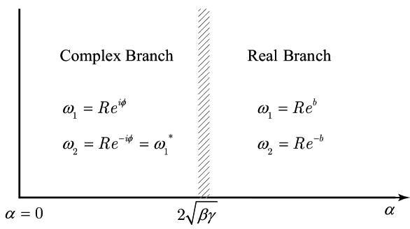
Figure 1 : Parameter branches.
The parameters have three branches and are shown in Figure 1
•
Complex branch α < 2 β γ 𝛼 2 𝛽 𝛾 \alpha<2\sqrt{\beta\gamma}
Frequencies ω 1 , ω 2 subscript 𝜔 1 subscript 𝜔 2
\omega_{1},\omega_{2}
ω 1 = ω 2 ∗ = R e i ϕ : R > 0 , ϕ ∈ [ − π / 2 , π / 2 ] : subscript 𝜔 1 superscript subscript 𝜔 2 𝑅 superscript 𝑒 𝑖 italic-ϕ formulae-sequence 𝑅 0 italic-ϕ 𝜋 2 𝜋 2 \displaystyle\omega_{1}=\omega_{2}^{*}=Re^{i\phi}~{}~{}:~{}~{}R>0,~{}~{}\phi\in[-\pi/2,\pi/2]
Note ϕ ∈ [ − π / 2 , π / 2 ] italic-ϕ 𝜋 2 𝜋 2 \phi\in[-\pi/2,\pi/2] α , β > 0 𝛼 𝛽
0 \alpha,\beta>0
•
Real branch α > 2 β γ 𝛼 2 𝛽 𝛾 \alpha>2\sqrt{\beta\gamma}
Frequencies ω 1 , ω 2 subscript 𝜔 1 subscript 𝜔 2
\omega_{1},\omega_{2} ω 1 > ω 2 subscript 𝜔 1 subscript 𝜔 2 \omega_{1}>\omega_{2}
ω 1 = R e b ; ω 2 = R e − b : R > 0 , b ∈ [ 0 , + ∞ ] : formulae-sequence subscript 𝜔 1 𝑅 superscript 𝑒 𝑏 subscript 𝜔 2 𝑅 superscript 𝑒 𝑏 formulae-sequence 𝑅 0 𝑏 0 \displaystyle\omega_{1}=Re^{b}~{}~{};~{}~{}\omega_{2}=Re^{-b}~{}~{}:~{}~{}R>0,~{}~{}b\in[0,+\infty]
For the case of real ω 1 subscript 𝜔 1 \omega_{1} ω 2 subscript 𝜔 2 \omega_{2} ω 1 > ω 2 subscript 𝜔 1 subscript 𝜔 2 \omega_{1}>\omega_{2}
ω 1 = 1 2 γ ( α + 2 γ β + α − 2 γ β ) subscript 𝜔 1 1 2 𝛾 𝛼 2 𝛾 𝛽 𝛼 2 𝛾 𝛽 \displaystyle\omega_{1}=\frac{1}{2\sqrt{\gamma}}\left(\sqrt{\alpha+2\sqrt{\gamma\beta}}+\sqrt{\alpha-2\sqrt{\gamma\beta}}\right)
ω 2 = 1 2 γ ( α + 2 γ β − α − 2 γ β ) subscript 𝜔 2 1 2 𝛾 𝛼 2 𝛾 𝛽 𝛼 2 𝛾 𝛽 \displaystyle\omega_{2}=\frac{1}{2\sqrt{\gamma}}\left(\sqrt{\alpha+2\sqrt{\gamma\beta}}-\sqrt{\alpha-2\sqrt{\gamma\beta}}\right)~{} (46)
ω 1 > ω 2 for ω 1 , ω 2 real subscript 𝜔 1 subscript 𝜔 2 for ω 1 , ω 2 real \displaystyle\omega_{1}>\omega_{2}~{}~{}\text{for $\omega_{1},~{}\omega_{2}$ real}
•
Equal frequency α = 2 β γ 𝛼 2 𝛽 𝛾 \alpha=2\sqrt{\beta\gamma}
ω 1 = ω 2 ; b = 0 = ϕ formulae-sequence subscript 𝜔 1 subscript 𝜔 2 𝑏 0 italic-ϕ \displaystyle\omega_{1}=\omega_{2}~{}~{};~{}~{}b=0=\phi
The special case of equal frequency ω 1 = ω 2 subscript 𝜔 1 subscript 𝜔 2 \omega_{1}=\omega_{2} [3 ] .
A similarity transformation is obtained such that
e − Q / 2 H e Q / 2 = H O superscript 𝑒 𝑄 2 𝐻 superscript 𝑒 𝑄 2 subscript 𝐻 𝑂 e^{-Q/2}He^{Q/2}=H_{O} (47)
where the Hamiltonian H O subscript 𝐻 𝑂 H_{O} x 𝑥 x v 𝑣 v
In a pioneering paper, Bender and Mannheim [5 ] found the operator Q 𝑄 Q
Q 𝑄 \displaystyle Q = a x v − b ∂ 2 ∂ x ∂ v absent 𝑎 𝑥 𝑣 𝑏 superscript 2 𝑥 𝑣 \displaystyle=axv-b\frac{\partial^{2}}{\partial x\partial v} (48)
For the real domain where ω 1 , ω 2 subscript 𝜔 1 subscript 𝜔 2
\omega_{1},~{}\omega_{2} a , b 𝑎 𝑏
a,b
Q 𝑄 \displaystyle Q = Q † : Hermitian for ω 1 , ω 2 real : absent superscript 𝑄 † Hermitian for ω 1 , ω 2 real \displaystyle=Q^{\dagger}:~{}~{}\text{Hermitian for $\omega_{1},~{}\omega_{2}$ real} (49)
The definition of Q 𝑄 Q Q 𝑄 Q
To obtain H 0 subscript 𝐻 0 H_{0}
e − Q 𝒪 e Q = ∑ n = 0 ∞ 1 n ! [ [ [ 𝒪 , Q ] , Q ] … Q ] ⏟ n − fold commutator superscript 𝑒 𝑄 𝒪 superscript 𝑒 𝑄 superscript subscript 𝑛 0 1 𝑛 subscript ⏟ delimited-[] 𝒪 𝑄 𝑄 … 𝑄 𝑛 fold commutator e^{-Q}\mathcal{O}e^{Q}=\displaystyle\sum_{n=0}^{\infty}\frac{1}{n!}\underbrace{\left[\left[[\mathcal{O},Q],Q\right]\ldots Q\right]}_{n-\text{fold commutator}} (50)
needs to be applied to 𝒪 = x , v , ∂ / ∂ x , ∂ / ∂ v 𝒪 𝑥 𝑣 𝑥 𝑣
\mathcal{O}=x,v,\partial/\partial x,\partial/\partial v
To obtain the commutator, note that the n 𝑛 n Q 𝑄 Q x , v , ∂ / ∂ x 𝑥 𝑣 𝑥
x,v,\partial/\partial x ∂ / ∂ v 𝑣 \partial/\partial v
[ x , Q ] = b ∂ ∂ v , 𝑥 𝑄 𝑏 𝑣 \displaystyle[x,Q]=b\frac{\partial}{\partial v}, [ [ x , Q ] , Q ] 𝑥 𝑄 𝑄 \displaystyle\left[[x,Q],Q\right] = a b x , absent 𝑎 𝑏 𝑥 \displaystyle=abx, … … \displaystyle\ldots
[ ∂ ∂ x , Q ] = a v , 𝑥 𝑄 𝑎 𝑣 \displaystyle[\frac{\partial}{\partial x},Q]=av, [ [ ∂ ∂ x , Q ] , Q ] 𝑥 𝑄 𝑄 \displaystyle\left[[\frac{\partial}{\partial x},Q],Q\right] = a b ∂ ∂ x , absent 𝑎 𝑏 𝑥 \displaystyle=ab\frac{\partial}{\partial x}, … … \displaystyle\ldots
[ v , Q ] = b ∂ ∂ x , 𝑣 𝑄 𝑏 𝑥 \displaystyle[v,Q]=b\frac{\partial}{\partial x}, [ [ v , Q ] , Q ] 𝑣 𝑄 𝑄 \displaystyle\left[[v,Q],Q\right] = a b v , absent 𝑎 𝑏 𝑣 \displaystyle=abv, … … \displaystyle\ldots
[ ∂ ∂ v , Q ] = a x , 𝑣 𝑄 𝑎 𝑥 \displaystyle[\frac{\partial}{\partial v},Q]=ax, [ [ ∂ ∂ v , Q ] , Q ] 𝑣 𝑄 𝑄 \displaystyle\left[[\frac{\partial}{\partial v},Q],Q\right] = a b ∂ ∂ v , absent 𝑎 𝑏 𝑣 \displaystyle=ab\frac{\partial}{\partial v}, … … \displaystyle\ldots
Carrying out the nested commutators to all orders and summing the result yields, for a , b > 0 𝑎 𝑏
0 a,b>0
e − τ Q x e τ Q superscript 𝑒 𝜏 𝑄 𝑥 superscript 𝑒 𝜏 𝑄 \displaystyle e^{-\tau Q}xe^{\tau Q} = cosh ( τ a b ) x + b a sinh ( τ a b ) ∂ ∂ v absent 𝜏 𝑎 𝑏 𝑥 𝑏 𝑎 𝜏 𝑎 𝑏 𝑣 \displaystyle=\cosh(\tau\sqrt{ab})x+\sqrt{\frac{b}{a}}\sinh(\tau\sqrt{ab})\frac{\partial}{\partial v}
e − τ Q ∂ ∂ x e τ Q superscript 𝑒 𝜏 𝑄 𝑥 superscript 𝑒 𝜏 𝑄 \displaystyle e^{-\tau Q}\frac{\partial}{\partial x}e^{\tau Q} = cosh ( τ a b ) ∂ ∂ x + a b sinh ( τ a b ) v absent 𝜏 𝑎 𝑏 𝑥 𝑎 𝑏 𝜏 𝑎 𝑏 𝑣 \displaystyle=\cosh(\tau\sqrt{ab})\frac{\partial}{\partial x}+\sqrt{\frac{a}{b}}\sinh(\tau\sqrt{ab})v
e − Q v e τ Q superscript 𝑒 𝑄 𝑣 superscript 𝑒 𝜏 𝑄 \displaystyle e^{-Q}ve^{\tau Q} = cosh ( τ a b ) v + b a sinh ( τ a b ) ∂ ∂ x absent 𝜏 𝑎 𝑏 𝑣 𝑏 𝑎 𝜏 𝑎 𝑏 𝑥 \displaystyle=\cosh(\tau\sqrt{ab})v+\sqrt{\frac{b}{a}}\sinh(\tau\sqrt{ab})\frac{\partial}{\partial x}
e τ − Q ∂ ∂ v e τ Q superscript 𝑒 𝜏 𝑄 𝑣 superscript 𝑒 𝜏 𝑄 \displaystyle e^{\tau-Q}\frac{\partial}{\partial v}e^{\tau Q} = cosh ( τ a b ) ∂ ∂ v + a b sinh ( τ a b ) x absent 𝜏 𝑎 𝑏 𝑣 𝑎 𝑏 𝜏 𝑎 𝑏 𝑥 \displaystyle=\cosh(\tau\sqrt{ab})\frac{\partial}{\partial v}+\sqrt{\frac{a}{b}}\sinh(\tau\sqrt{ab})x (51)
The Euclidean result given above is simpler that the Minkowski commutators, which have alternating signs and i 𝑖 i
Consider the following equation
e − Q / 2 H e Q / 2 = C 1 ∂ 2 ∂ v 2 + C 2 x ∂ ∂ v + C 3 v ∂ ∂ x + C 4 ∂ 2 ∂ x 2 + C 5 x 2 + C 6 v 2 superscript 𝑒 𝑄 2 𝐻 superscript 𝑒 𝑄 2 subscript 𝐶 1 superscript 2 superscript 𝑣 2 subscript 𝐶 2 𝑥 𝑣 subscript 𝐶 3 𝑣 𝑥 subscript 𝐶 4 superscript 2 superscript 𝑥 2 subscript 𝐶 5 superscript 𝑥 2 subscript 𝐶 6 superscript 𝑣 2 e^{-Q/2}He^{Q/2}=C_{1}\frac{\partial^{2}}{\partial v^{2}}+C_{2}x\frac{\partial}{\partial v}+C_{3}v\frac{\partial}{\partial x}+C_{4}\frac{\partial^{2}}{\partial x^{2}}+C_{5}x^{2}+C_{6}v^{2} (52)
To obtain the factorization of the Hamiltonian into two de-coupled oscillators, choose the following values for a 𝑎 a b 𝑏 b
a b = γ ω 1 ω 2 ; sinh ( a b ) = 2 ω 1 ω 2 ω 1 2 − ω 2 2 ⇒ a b = ln ( ω 1 + ω 2 ω 1 − ω 2 ) formulae-sequence 𝑎 𝑏 𝛾 subscript 𝜔 1 subscript 𝜔 2 𝑎 𝑏 2 subscript 𝜔 1 subscript 𝜔 2 superscript subscript 𝜔 1 2 superscript subscript 𝜔 2 2 ⇒ 𝑎 𝑏 subscript 𝜔 1 subscript 𝜔 2 subscript 𝜔 1 subscript 𝜔 2 \sqrt{\frac{a}{b}}=\gamma\omega_{1}\omega_{2};~{}~{}\sinh(\sqrt{ab})=\frac{2\omega_{1}\omega_{2}}{\omega_{1}^{2}-\omega_{2}^{2}}~{}~{}\Rightarrow~{}~{}\sqrt{ab}=\ln\left(\frac{\omega_{1}+\omega_{2}}{\omega_{1}-\omega_{2}}\right) (53)
Note the definition of a 𝑎 a b 𝑏 b ω 1 , ω 2 subscript 𝜔 1 subscript 𝜔 2
\omega_{1},\omega_{2} ω 1 > ω 2 subscript 𝜔 1 subscript 𝜔 2 \omega_{1}>\omega_{2} Q 𝑄 Q
Define
A = cosh ( a b 2 ) 𝐴 𝑎 𝑏 2 \displaystyle A=\cosh(\frac{\sqrt{ab}}{2}) = ω 1 ω 1 2 − ω 2 2 ; B = sinh ( a b 2 ) = ω 2 ω 1 2 − ω 2 2 formulae-sequence absent subscript 𝜔 1 superscript subscript 𝜔 1 2 superscript subscript 𝜔 2 2 𝐵 𝑎 𝑏 2 subscript 𝜔 2 superscript subscript 𝜔 1 2 superscript subscript 𝜔 2 2 \displaystyle=\frac{\omega_{1}}{\sqrt{\omega_{1}^{2}-\omega_{2}^{2}}}~{}~{};~{}~{}B=\sinh(\frac{\sqrt{ab}}{2})=\frac{\omega_{2}}{\sqrt{\omega_{1}^{2}-\omega_{2}^{2}}} (54)
C 𝐶 \displaystyle~{}C = a b = γ ω 1 ω 2 absent 𝑎 𝑏 𝛾 subscript 𝜔 1 subscript 𝜔 2 \displaystyle=\sqrt{\frac{a}{b}}=\gamma\omega_{1}\omega_{2}
Using the result of Eq. 5 52
C 1 subscript 𝐶 1 \displaystyle C_{1} = − 1 2 γ A 2 + γ 2 ( B C ) 2 ω 1 2 ω 2 2 absent 1 2 𝛾 superscript 𝐴 2 𝛾 2 superscript 𝐵 𝐶 2 superscript subscript 𝜔 1 2 superscript subscript 𝜔 2 2 \displaystyle=-\frac{1}{2\gamma}A^{2}+\frac{\gamma}{2}\left(\frac{B}{C}\right)^{2}\omega_{1}^{2}\omega_{2}^{2}
= − 1 2 γ [ cosh 2 ( a b 2 ) − sinh 2 ( a b 2 ) ] absent 1 2 𝛾 delimited-[] superscript 2 𝑎 𝑏 2 superscript 2 𝑎 𝑏 2 \displaystyle=-\frac{1}{2\gamma}\left[\cosh^{2}\left(\frac{\sqrt{ab}}{2}\right)-\sinh^{2}\left(\frac{\sqrt{ab}}{2}\right)\right]
= − 1 2 γ absent 1 2 𝛾 \displaystyle=-\frac{1}{2\gamma} (55)
Similarly, after some simplifications
C 2 subscript 𝐶 2 \displaystyle C_{2} = − C A B γ + γ ω 1 2 ω 2 2 ( A B C ) = 0 absent 𝐶 𝐴 𝐵 𝛾 𝛾 superscript subscript 𝜔 1 2 superscript subscript 𝜔 2 2 𝐴 𝐵 𝐶 0 \displaystyle=-\frac{CAB}{\gamma}+\gamma\omega_{1}^{2}\omega_{2}^{2}\left(\frac{AB}{C}\right)=0
C 3 subscript 𝐶 3 \displaystyle C_{3} = − ( A 2 + B 2 ) + γ ( ω 1 2 + ω 2 2 ) ( A B C ) = 0 absent superscript 𝐴 2 superscript 𝐵 2 𝛾 superscript subscript 𝜔 1 2 superscript subscript 𝜔 2 2 𝐴 𝐵 𝐶 0 \displaystyle=-(A^{2}+B^{2})+\gamma(\omega_{1}^{2}+\omega_{2}^{2})\left(\frac{AB}{C}\right)=0
The constants a 𝑎 a b 𝑏 b C 2 = C 3 = 0 subscript 𝐶 2 subscript 𝐶 3 0 C_{2}=C_{3}=0
C 2 = C 3 = 0 ⇒ Determines a and b subscript 𝐶 2 subscript 𝐶 3 0 ⇒ Determines 𝑎 and 𝑏 C_{2}=C_{3}=0~{}~{}\Rightarrow~{}~{}~{}\text{Determines}~{}a~{}\text{and}~{}b (56)
The remaining coefficients are given by
C 4 subscript 𝐶 4 \displaystyle C_{4} = − A B C + γ 2 ( ω 1 2 + ω 2 2 ) ( B C ) 2 = − 1 2 γ ω 1 2 absent 𝐴 𝐵 𝐶 𝛾 2 superscript subscript 𝜔 1 2 superscript subscript 𝜔 2 2 superscript 𝐵 𝐶 2 1 2 𝛾 superscript subscript 𝜔 1 2 \displaystyle=-\frac{AB}{C}+\frac{\gamma}{2}(\omega_{1}^{2}+\omega_{2}^{2})\left(\frac{B}{C}\right)^{2}=-\frac{1}{2\gamma\omega_{1}^{2}}
C 5 subscript 𝐶 5 \displaystyle C_{5} = − 1 2 γ B 2 C 2 + γ 2 ω 1 2 ω 2 2 A 2 = γ 2 ω 1 2 ω 2 2 absent 1 2 𝛾 superscript 𝐵 2 superscript 𝐶 2 𝛾 2 superscript subscript 𝜔 1 2 superscript subscript 𝜔 2 2 superscript 𝐴 2 𝛾 2 superscript subscript 𝜔 1 2 superscript subscript 𝜔 2 2 \displaystyle=-\frac{1}{2\gamma}B^{2}C^{2}+\frac{\gamma}{2}\omega_{1}^{2}\omega_{2}^{2}A^{2}=\frac{\gamma}{2}\omega_{1}^{2}\omega_{2}^{2}
C 6 subscript 𝐶 6 \displaystyle C_{6} = − A B C + γ 2 ( ω 1 2 + ω 2 2 ) A 2 = γ 2 ω 1 2 absent 𝐴 𝐵 𝐶 𝛾 2 superscript subscript 𝜔 1 2 superscript subscript 𝜔 2 2 superscript 𝐴 2 𝛾 2 superscript subscript 𝜔 1 2 \displaystyle=-ABC+\frac{\gamma}{2}(\omega_{1}^{2}+\omega_{2}^{2})A^{2}=\frac{\gamma}{2}\omega_{1}^{2} (57)
Collecting all the results yields
e − Q / 2 H e Q / 2 superscript 𝑒 𝑄 2 𝐻 superscript 𝑒 𝑄 2 \displaystyle e^{-Q/2}He^{Q/2} = H O absent subscript 𝐻 𝑂 \displaystyle=H_{O} (58)
= − 1 2 γ ∂ 2 ∂ v 2 − 1 2 γ ω 1 2 ∂ 2 ∂ x 2 + γ 2 ω 1 2 v 2 + γ 2 ω 1 2 ω 2 2 x 2 absent 1 2 𝛾 superscript 2 superscript 𝑣 2 1 2 𝛾 superscript subscript 𝜔 1 2 superscript 2 superscript 𝑥 2 𝛾 2 superscript subscript 𝜔 1 2 superscript 𝑣 2 𝛾 2 superscript subscript 𝜔 1 2 superscript subscript 𝜔 2 2 superscript 𝑥 2 \displaystyle=-\frac{1}{2\gamma}\frac{\partial^{2}}{\partial v^{2}}-\frac{1}{2\gamma\omega_{1}^{2}}\frac{\partial^{2}}{\partial x^{2}}+\frac{\gamma}{2}\omega_{1}^{2}v^{2}+\frac{\gamma}{2}\omega_{1}^{2}\omega_{2}^{2}x^{2} (59)
6 The matrix elements of e − τ Q superscript 𝑒 𝜏 𝑄 e^{-\tau Q}
The Q 𝑄 Q 48
Q = a x v − b ∂ 2 ∂ x ∂ v 𝑄 𝑎 𝑥 𝑣 𝑏 superscript 2 𝑥 𝑣 Q=axv-b\frac{\partial^{2}}{\partial x\partial v} (60)
where, from Eq. 53
a b = γ ω 1 ω 2 ; sinh ( a b ) = 2 ω 1 ω 2 ω 1 2 − ω 2 2 formulae-sequence 𝑎 𝑏 𝛾 subscript 𝜔 1 subscript 𝜔 2 𝑎 𝑏 2 subscript 𝜔 1 subscript 𝜔 2 superscript subscript 𝜔 1 2 superscript subscript 𝜔 2 2 \sqrt{\frac{a}{b}}=\gamma\omega_{1}\omega_{2}~{};\quad\sinh(\sqrt{ab})=\frac{2\omega_{1}\omega_{2}}{\omega_{1}^{2}-\omega_{2}^{2}}
The finite matrix elements of the e ± τ Q superscript 𝑒 plus-or-minus 𝜏 𝑄 e^{\pm\tau Q} Q 𝑄 Q
Consider the change of variables given by
α 𝛼 \displaystyle\alpha = 1 2 ( x + v ) ; β = 1 2 ( x − v ) formulae-sequence absent 1 2 𝑥 𝑣 𝛽 1 2 𝑥 𝑣 \displaystyle=\frac{1}{\sqrt{2}}(x+v)~{};\quad\beta=\frac{1}{\sqrt{2}}(x-v) (61)
∂ ∂ x 𝑥 \displaystyle\frac{\partial}{\partial x} = 1 2 ( ∂ ∂ α + ∂ ∂ β ) ; ∂ ∂ v = 1 2 ( ∂ ∂ α − ∂ ∂ β ) formulae-sequence absent 1 2 𝛼 𝛽 𝑣 1 2 𝛼 𝛽 \displaystyle=\frac{1}{\sqrt{2}}(\frac{\partial}{\partial\alpha}+\frac{\partial}{\partial\beta})~{};\quad\frac{\partial}{\partial v}=\frac{1}{\sqrt{2}}(\frac{\partial}{\partial\alpha}-\frac{\partial}{\partial\beta}) (62)
In these coordinates the α , β 𝛼 𝛽
\alpha,~{}\beta
Q 𝑄 \displaystyle Q = a 2 ( α 2 − β 2 ) − b 2 ( ∂ 2 ∂ α 2 − ∂ 2 ∂ β 2 ) absent 𝑎 2 superscript 𝛼 2 superscript 𝛽 2 𝑏 2 superscript 2 superscript 𝛼 2 superscript 2 superscript 𝛽 2 \displaystyle=\frac{a}{2}(\alpha^{2}-\beta^{2})-\frac{b}{2}(\frac{\partial^{2}}{\partial\alpha^{2}}-\frac{\partial^{2}}{\partial\beta^{2}})
= − 1 2 b ∂ 2 ∂ α 2 + 1 2 a α 2 + 1 2 b ∂ 2 ∂ β 2 − 1 2 a β 2 absent 1 2 𝑏 superscript 2 superscript 𝛼 2 1 2 𝑎 superscript 𝛼 2 1 2 𝑏 superscript 2 superscript 𝛽 2 1 2 𝑎 superscript 𝛽 2 \displaystyle=-\frac{1}{2}b\frac{\partial^{2}}{\partial\alpha^{2}}+\frac{1}{2}a\alpha^{2}+\frac{1}{2}b\frac{\partial^{2}}{\partial\beta^{2}}-\frac{1}{2}a\beta^{2} (63)
Consider the Hamiltonian of a quantum oscillator given by
H sho = − 1 2 m ∂ 2 ∂ z 2 + 1 2 m ω 2 z 2 subscript 𝐻 sho 1 2 𝑚 superscript 2 superscript 𝑧 2 1 2 𝑚 superscript 𝜔 2 superscript 𝑧 2 H_{\text{sho}}=-\frac{1}{2m}\frac{\partial^{2}}{\partial z^{2}}+\frac{1}{2}m\omega^{2}z^{2} (64)
with the transition amplitude given by [11 ]
K ( z , z ′ ; τ ) = ⟨ z | e − τ H | z ′ ⟩ 𝐾 𝑧 superscript 𝑧 ′ 𝜏 quantum-operator-product 𝑧 superscript 𝑒 𝜏 𝐻 superscript 𝑧 ′ \displaystyle K(z,z^{\prime};\tau)=\langle z|e^{-\tau H}|z^{\prime}\rangle
= m ω 2 π sinh ω τ exp { − m ω 2 sinh ( ω τ ) [ ( z 2 + z ′ 2 ) cosh ( ω τ ) − 2 z z ′ ] } absent 𝑚 𝜔 2 𝜋 𝜔 𝜏 𝑚 𝜔 2 𝜔 𝜏 delimited-[] superscript 𝑧 2 superscript 𝑧 ′ 2
𝜔 𝜏 2 𝑧 superscript 𝑧 ′ \displaystyle=\sqrt{\frac{m\omega}{2\pi\sinh{\omega\tau}}}\exp\left\{-\frac{m\omega}{2\sinh(\omega\tau)}\Big{[}(z^{2}+z^{\prime 2})\cosh(\omega\tau)-2zz^{\prime}\Big{]}\right\} (65)
Comparing the α 𝛼 \alpha β 𝛽 \beta Q 𝑄 Q H sho subscript 𝐻 sho H_{\text{sho}} a , b 𝑎 𝑏
a,b α 𝛼 \alpha β 𝛽 \beta β 𝛽 \beta
To exploit the quadratic form of the α 𝛼 \alpha β 𝛽 \beta m 𝑚 m
α − sector : : 𝛼 sector absent \displaystyle\alpha-\mathrm{sector}: b 𝑏 \displaystyle b = 1 m ; absent 1 𝑚 \displaystyle=\frac{1}{m}; a 𝑎 \displaystyle a = m ω 2 absent 𝑚 superscript 𝜔 2 \displaystyle=m\omega^{2} ⇒ ⇒ \displaystyle\Rightarrow ω 𝜔 \displaystyle\omega = a b absent 𝑎 𝑏 \displaystyle=\sqrt{ab} (66)
β − sector : : 𝛽 sector absent \displaystyle\beta-\mathrm{sector}: b 𝑏 \displaystyle b = − 1 m ; absent 1 𝑚 \displaystyle=-\frac{1}{m}; a 𝑎 \displaystyle a = − m ω 2 absent 𝑚 superscript 𝜔 2 \displaystyle=-m\omega^{2} ⇒ ⇒ \displaystyle\Rightarrow ω 𝜔 \displaystyle\omega = a b absent 𝑎 𝑏 \displaystyle=\sqrt{ab} (67)
Hence Eqs. 63 65 67
⟨ α , β | e − τ Q | α ′ , β ′ ⟩ quantum-operator-product 𝛼 𝛽
superscript 𝑒 𝜏 𝑄 superscript 𝛼 ′ superscript 𝛽 ′
\displaystyle\langle\alpha,\beta|e^{-\tau Q}|\alpha^{\prime},\beta^{\prime}\rangle
= N α N β exp { − 1 2 b a b sinh ( τ a b ) [ ( α 2 + α ′ 2 ) cosh ( τ a b ) − 2 α α ′ ] } absent subscript 𝑁 𝛼 subscript 𝑁 𝛽 1 2 𝑏 𝑎 𝑏 𝜏 𝑎 𝑏 delimited-[] superscript 𝛼 2 superscript 𝛼 ′ 2
𝜏 𝑎 𝑏 2 𝛼 superscript 𝛼 ′ \displaystyle=N_{\alpha}N_{\beta}\exp\left\{-\frac{1}{2b}\frac{\sqrt{ab}}{\sinh(\tau\sqrt{ab})}\big{[}(\alpha^{2}+\alpha^{\prime 2})\cosh(\tau\sqrt{ab})-2\alpha\alpha^{\prime}\big{]}\right\}
× exp { 1 2 b a b sinh ( τ a b ) [ ( β 2 + β ′ 2 ) cosh ( τ a b ) − 2 β β ′ ] } absent 1 2 𝑏 𝑎 𝑏 𝜏 𝑎 𝑏 delimited-[] superscript 𝛽 2 superscript 𝛽 ′ 2
𝜏 𝑎 𝑏 2 𝛽 superscript 𝛽 ′ \displaystyle\qquad\times\exp\left\{\frac{1}{2b}\frac{\sqrt{ab}}{\sinh(\tau\sqrt{ab})}\big{[}(\beta^{2}+\beta^{\prime 2})\cosh(\tau\sqrt{ab})-2\beta\beta^{\prime}\big{]}\right\}
= 𝒩 ( τ ) exp { − 1 2 𝒢 ( τ ) ( α 2 + α ′ 2 − β 2 − β ′ 2 ) + ℋ ( τ ) ( α α ′ − β β ′ ) } absent 𝒩 𝜏 1 2 𝒢 𝜏 superscript 𝛼 2 superscript 𝛼 ′ 2
superscript 𝛽 2 superscript 𝛽 ′ 2
ℋ 𝜏 𝛼 superscript 𝛼 ′ 𝛽 superscript 𝛽 ′ \displaystyle=\mathcal{N}(\tau)\exp\Big{\{}-\frac{1}{2}\mathcal{G}(\tau)(\alpha^{2}+\alpha^{\prime 2}-\beta^{2}-\beta^{\prime 2})+\mathcal{H}(\tau)(\alpha\alpha^{\prime}-\beta\beta^{\prime})\Big{\}}
where
𝒢 ( τ ) = a b coth ( τ a b ) ; ℋ ( τ ) = a b 1 sinh ( τ a b ) formulae-sequence 𝒢 𝜏 𝑎 𝑏 hyperbolic-cotangent 𝜏 𝑎 𝑏 ℋ 𝜏 𝑎 𝑏 1 𝜏 𝑎 𝑏 \displaystyle\mathcal{G}(\tau)=\sqrt{\frac{a}{b}}\coth(\tau\sqrt{ab})~{};\quad\mathcal{H}(\tau)=\sqrt{\frac{a}{b}}\frac{1}{\sinh(\tau\sqrt{ab})} (68)
and
𝒩 ( τ ) = a b 2 π b sinh ( τ a b ) ⋅ a b − 2 π b sinh ( τ a b ) 𝒩 𝜏 ⋅ 𝑎 𝑏 2 𝜋 𝑏 𝜏 𝑎 𝑏 𝑎 𝑏 2 𝜋 𝑏 𝜏 𝑎 𝑏 \displaystyle\mathcal{N}(\tau)=\sqrt{\frac{\sqrt{ab}}{2\pi b\sinh(\tau\sqrt{ab})}}\cdot\sqrt{\frac{\sqrt{ab}}{-2\pi b\sinh(\tau\sqrt{ab})}}
⇒ 𝒩 ( τ ) = i 2 π a b 1 | sinh ( τ a b ) | = i 2 π | ℋ ( τ ) | ⇒ absent 𝒩 𝜏 𝑖 2 𝜋 𝑎 𝑏 1 𝜏 𝑎 𝑏 𝑖 2 𝜋 ℋ 𝜏 \displaystyle\Rightarrow\mathcal{N}(\tau)=\frac{i}{2\pi}\sqrt{\frac{a}{b}}\frac{1}{|\sinh(\tau\sqrt{ab})|}=\frac{i}{2\pi}\big{|}\mathcal{H}(\tau)\big{|} (69)
Hence a heuristic derivation for Q 𝑄 Q
⟨ x , v | e − τ Q | x ′ , v ′ ⟩ = 𝒩 ( τ ) exp { − 𝒢 ( τ ) ( x v + x ′ v ′ ) + ℋ ( τ ) ( x v ′ + v x ′ ) } quantum-operator-product 𝑥 𝑣
superscript 𝑒 𝜏 𝑄 superscript 𝑥 ′ superscript 𝑣 ′
𝒩 𝜏 𝒢 𝜏 𝑥 𝑣 superscript 𝑥 ′ superscript 𝑣 ′ ℋ 𝜏 𝑥 superscript 𝑣 ′ 𝑣 superscript 𝑥 ′ \displaystyle\langle x,v|e^{-\tau Q}|x^{\prime},v^{\prime}\rangle=\mathcal{N}(\tau)\exp\left\{-\mathcal{G}(\tau)(xv+x^{\prime}v^{\prime})+\mathcal{H}(\tau)(xv^{\prime}+vx^{\prime})\right\} (70)
The normalization constant 𝒩 ( τ ) 𝒩 𝜏 \mathcal{N}(\tau) H 𝐻 H
For the real branch, both coefficients 𝒢 ( τ ) 𝒢 𝜏 \mathcal{G}(\tau) ℋ ( τ ) ℋ 𝜏 \mathcal{H}(\tau) Q = Q † 𝑄 superscript 𝑄 † Q=Q^{\dagger}
Note the form obtained for e − τ Q superscript 𝑒 𝜏 𝑄 e^{-\tau Q} 70 Q 𝑄 Q 4 + 12 = 16 4 12 16 4+12=16 70 e − τ Q superscript 𝑒 𝜏 𝑄 e^{-\tau Q} 𝒢 ( τ ) 𝒢 𝜏 \mathcal{G}(\tau) ℋ ( τ ) ℋ 𝜏 \mathcal{H}(\tau) 𝒩 ( τ ) 𝒩 𝜏 \mathcal{N}(\tau)
The operator Q 𝑄 Q e − τ Q e τ Q = 𝕀 superscript 𝑒 𝜏 𝑄 superscript 𝑒 𝜏 𝑄 𝕀 e^{-\tau Q}e^{\tau Q}=\mathbb{I} e − τ Q e τ Q superscript 𝑒 𝜏 𝑄 superscript 𝑒 𝜏 𝑄 e^{-\tau Q}e^{\tau Q}
⟨ x , v | e − τ Q e τ Q | x ′ , v ′ ⟩ = ∫ 𝑑 ξ 𝑑 ζ ⟨ x , v | e − τ Q | ξ , ζ ⟩ ⟨ ξ , ζ | e τ Q | x ′ , v ′ ⟩ quantum-operator-product 𝑥 𝑣
superscript 𝑒 𝜏 𝑄 superscript 𝑒 𝜏 𝑄 superscript 𝑥 ′ superscript 𝑣 ′
differential-d 𝜉 differential-d 𝜁 quantum-operator-product 𝑥 𝑣
superscript 𝑒 𝜏 𝑄 𝜉 𝜁
quantum-operator-product 𝜉 𝜁
superscript 𝑒 𝜏 𝑄 superscript 𝑥 ′ superscript 𝑣 ′
\displaystyle\langle x,v|e^{-\tau Q}e^{\tau Q}|x^{\prime},v^{\prime}\rangle=\int d\xi d\zeta\langle x,v|e^{-\tau Q}|\xi,\zeta\rangle\langle\xi,\zeta|e^{\tau Q}|x^{\prime},v^{\prime}\rangle
= 𝒩 2 ( τ ) ∫ 𝑑 ξ 𝑑 ζ e − 𝒢 ( τ ) ( x v + ξ ζ ) + ℋ ( τ ) ( x ζ + v ξ ) e 𝒢 ( τ ) ( ξ ζ + x ′ v ′ ) − ℋ ( τ ) ( ξ v ′ + ζ x ′ ) absent superscript 𝒩 2 𝜏 differential-d 𝜉 differential-d 𝜁 superscript 𝑒 𝒢 𝜏 𝑥 𝑣 𝜉 𝜁 ℋ 𝜏 𝑥 𝜁 𝑣 𝜉 superscript 𝑒 𝒢 𝜏 𝜉 𝜁 superscript 𝑥 ′ superscript 𝑣 ′ ℋ 𝜏 𝜉 superscript 𝑣 ′ 𝜁 superscript 𝑥 ′ \displaystyle=\mathcal{N}^{2}(\tau)\int d\xi d\zeta e^{-\mathcal{G}(\tau)(xv+\xi\zeta)+\mathcal{H}(\tau)(x\zeta+v\xi)}e^{\mathcal{G}(\tau)(\xi\zeta+x^{\prime}v^{\prime})-\mathcal{H}(\tau)(\xi v^{\prime}+\zeta x^{\prime})}
= 𝒩 2 ( τ ) e − 𝒢 ( τ ) ( x v − x ′ v ′ ) ∫ 𝑑 ξ 𝑑 ζ exp { i ℋ ( τ ) i ξ ( v ′ − v ) + i ℋ ( τ ) i ζ ( x ′ − x ) } absent superscript 𝒩 2 𝜏 superscript 𝑒 𝒢 𝜏 𝑥 𝑣 superscript 𝑥 ′ superscript 𝑣 ′ differential-d 𝜉 differential-d 𝜁 𝑖 ℋ 𝜏 𝑖 𝜉 superscript 𝑣 ′ 𝑣 𝑖 ℋ 𝜏 𝑖 𝜁 superscript 𝑥 ′ 𝑥 \displaystyle=\mathcal{N}^{2}(\tau)e^{-\mathcal{G}(\tau)(xv-x^{\prime}v^{\prime})}\int d\xi d\zeta\exp\{i\mathcal{H}(\tau)i\xi(v^{\prime}-v)+i\mathcal{H}(\tau)i\zeta(x^{\prime}-x)\}
= 𝒩 2 ( τ ) ( 2 π i ℋ ( τ ) ) 2 δ ( x − x ′ ) δ ( v − v ′ ) = δ ( x − x ′ ) δ ( v − v ′ ) absent superscript 𝒩 2 𝜏 superscript 2 𝜋 𝑖 ℋ 𝜏 2 𝛿 𝑥 superscript 𝑥 ′ 𝛿 𝑣 superscript 𝑣 ′ 𝛿 𝑥 superscript 𝑥 ′ 𝛿 𝑣 superscript 𝑣 ′ \displaystyle=\mathcal{N}^{2}(\tau)\left(\frac{2\pi}{i\mathcal{H}(\tau)}\right)^{2}\delta(x-x^{\prime})\delta(v-v^{\prime})=\delta(x-x^{\prime})\delta(v-v^{\prime})
Hence
e − τ Q e τ Q = 𝕀 superscript 𝑒 𝜏 𝑄 superscript 𝑒 𝜏 𝑄 𝕀 \displaystyle e^{-\tau Q}e^{\tau Q}=\mathbb{I} (71)
To make the above derivation more rigorous one can analytically continue τ 𝜏 \tau t = − i τ 𝑡 𝑖 𝜏 t=-i\tau τ 𝜏 \tau
7 Vacuum state; e ± Q / 2 superscript 𝑒 plus-or-minus 𝑄 2 e^{\pm Q/2}
The vacuum state and the dual vacuum state of the Euclidean Hamiltonian is obtained using the expression for e Q / 2 superscript 𝑒 𝑄 2 e^{Q/2} e − Q / 2 superscript 𝑒 𝑄 2 e^{-Q/2} H 𝐻 H H † superscript 𝐻 † H^{\dagger} Q 𝑄 Q 6
From the oscillator Hamiltonian H 0 subscript 𝐻 0 H_{0} 59
H 0 | 0 , 0 ⟩ = 1 2 ( ω 1 + ω 2 ) | 0 , 0 ⟩ subscript 𝐻 0 ket 0 0
1 2 subscript 𝜔 1 subscript 𝜔 2 ket 0 0
\displaystyle H_{0}|0,0\rangle=\frac{1}{2}(\omega_{1}+\omega_{2})|0,0\rangle
⟨ x , v | 0 , 0 ⟩ = ( γ 2 ω 1 3 ω 2 π 2 ) 1 / 4 exp { − γ 2 ( ω 1 v 2 + ω 1 2 ω 2 x 2 ) } inner-product 𝑥 𝑣
0 0
superscript superscript 𝛾 2 superscript subscript 𝜔 1 3 subscript 𝜔 2 superscript 𝜋 2 1 4 𝛾 2 subscript 𝜔 1 superscript 𝑣 2 superscript subscript 𝜔 1 2 subscript 𝜔 2 superscript 𝑥 2 \displaystyle\langle x,v|0,0\rangle=\left(\frac{\gamma^{2}\omega_{1}^{3}\omega_{2}}{\pi^{2}}\right)^{1/4}\exp\left\{-\frac{\gamma}{2}(\omega_{1}v^{2}+\omega_{1}^{2}\omega_{2}x^{2})\right\}
The vacuum state is given by
| Ψ 00 ⟩ = e Q / 2 | 0 , 0 ⟩ ; H | Ψ 00 ⟩ = E 0 | Ψ 00 ⟩ ; E 00 = 1 2 [ ω 1 + ω 2 ] formulae-sequence ket subscript Ψ 00 superscript 𝑒 𝑄 2 ket 0 0
formulae-sequence 𝐻 ket subscript Ψ 00 subscript 𝐸 0 ket subscript Ψ 00 subscript 𝐸 00 1 2 delimited-[] subscript 𝜔 1 subscript 𝜔 2 \displaystyle|\Psi_{00}\rangle=e^{Q/2}|0,0\rangle~{};~{}H|\Psi_{00}\rangle=E_{0}|\Psi_{00}\rangle~{};~{}E_{00}=\frac{1}{2}[\omega_{1}+\omega_{2}] (72)
The co-ordinate representation of the vacuum state can be directly obtained from the Hamiltonian H 𝐻 H [4 ]
Ψ 00 ( x , v ) = ⟨ x , v | Ψ 00 ⟩ = ⟨ x , v | e Q / 2 | 0 , 0 ⟩ subscript Ψ 00 𝑥 𝑣 inner-product 𝑥 𝑣
subscript Ψ 00 quantum-operator-product 𝑥 𝑣
superscript 𝑒 𝑄 2 0 0
\displaystyle\Psi_{00}(x,v)=\langle x,v|\Psi_{00}\rangle=\langle x,v|e^{Q/2}|0,0\rangle
= N 00 exp { − γ 2 ( ω 1 + ω 2 ) ω 1 ω 2 x 2 − γ 2 ( ω 1 + ω 2 ) v 2 − γ ω 1 ω 2 x v } absent subscript 𝑁 00 𝛾 2 subscript 𝜔 1 subscript 𝜔 2 subscript 𝜔 1 subscript 𝜔 2 superscript 𝑥 2 𝛾 2 subscript 𝜔 1 subscript 𝜔 2 superscript 𝑣 2 𝛾 subscript 𝜔 1 subscript 𝜔 2 𝑥 𝑣 \displaystyle~{}~{}~{}=N_{00}\exp\left\{-\frac{\gamma}{2}(\omega_{1}+\omega_{2})\omega_{1}\omega_{2}x^{2}-\frac{\gamma}{2}(\omega_{1}+\omega_{2})v^{2}-\gamma\omega_{1}\omega_{2}xv\right\} (73)
The vacuum state | Ψ 00 ⟩ ket subscript Ψ 00 |\Psi_{00}\rangle N 00 subscript 𝑁 00 N_{00}
It can be directly verified that the dual ground state, from Eq. 7
Ψ 00 D ( x , v ) = N 00 exp { − γ 2 ( ω 1 + ω 2 ) ω 1 ω 2 x 2 − γ 2 ( ω 1 + ω 2 ) v 2 + γ ω 1 ω 2 x v } superscript subscript Ψ 00 𝐷 𝑥 𝑣 subscript 𝑁 00 𝛾 2 subscript 𝜔 1 subscript 𝜔 2 subscript 𝜔 1 subscript 𝜔 2 superscript 𝑥 2 𝛾 2 subscript 𝜔 1 subscript 𝜔 2 superscript 𝑣 2 𝛾 subscript 𝜔 1 subscript 𝜔 2 𝑥 𝑣 \displaystyle\Psi_{00}^{D}(x,v)=N_{00}\exp\left\{-\frac{\gamma}{2}(\omega_{1}+\omega_{2})\omega_{1}\omega_{2}x^{2}-\frac{\gamma}{2}(\omega_{1}+\omega_{2})v^{2}+\gamma\omega_{1}\omega_{2}xv\right\}
More formally, the dual vacuum state obeys the following
⟨ Ψ 00 D | = ⟨ 0 , 0 | e − Q / 2 bra subscript superscript Ψ 𝐷 00 bra 0 0
superscript 𝑒 𝑄 2 \displaystyle\langle\Psi^{D}_{00}|=\langle 0,0|e^{-Q/2}~{}~{}~{}~{}~{}~{}~{}~{}~{}~{}~{}~{}
⇒ ⇒ \displaystyle\Rightarrow~{}~{} Ψ 00 D ( x , v ) = ⟨ Ψ 00 D | x , v ⟩ = ⟨ 0 , 0 | e − Q / 2 | x , v ⟩ subscript superscript Ψ 𝐷 00 𝑥 𝑣 inner-product subscript superscript Ψ 𝐷 00 𝑥 𝑣
quantum-operator-product 0 0
superscript 𝑒 𝑄 2 𝑥 𝑣
\displaystyle\Psi^{D}_{00}(x,v)=\langle\Psi^{D}_{00}|x,v\rangle=\langle 0,0|e^{-Q/2}|x,v\rangle
From Eq. 70 τ = − 1 / 2 𝜏 1 2 \tau=-1/2
⟨ x , v | e Q / 2 | x ′ , v ′ ⟩ = quantum-operator-product 𝑥 𝑣
superscript 𝑒 𝑄 2 superscript 𝑥 ′ superscript 𝑣 ′
absent \displaystyle\langle x,v|e^{Q/2}|x^{\prime},v^{\prime}\rangle=~{}~{}~{}~{}~{}~{}~{}~{}~{}~{}~{}~{}~{}~{}~{}~{}~{}~{}~{}~{}~{}~{}~{}~{}~{}~{}~{}~{}~{}~{}
𝒩 ( 1 2 ) exp { a b coth ( a b 2 ) ( x v + x ′ v ′ ) − a b ( x v ′ + v x ′ ) sinh ( a b 2 ) } 𝒩 1 2 𝑎 𝑏 hyperbolic-cotangent 𝑎 𝑏 2 𝑥 𝑣 superscript 𝑥 ′ superscript 𝑣 ′ 𝑎 𝑏 𝑥 superscript 𝑣 ′ 𝑣 superscript 𝑥 ′ 𝑎 𝑏 2 \displaystyle\mathcal{N}(\frac{1}{2})\exp\left\{\sqrt{\frac{a}{b}}\coth\left(\frac{\sqrt{ab}}{2}\right)(xv+x^{\prime}v^{\prime})-\sqrt{\frac{a}{b}}\frac{(xv^{\prime}+vx^{\prime})}{\sinh\left(\frac{\sqrt{ab}}{2}\right)}\right\} (74)
Note
a b coth ( a b 2 ) = γ ω 1 2 ; a b 1 sinh ( a b 2 ) = γ ω 1 ω 1 2 − ω 2 2 formulae-sequence 𝑎 𝑏 hyperbolic-cotangent 𝑎 𝑏 2 𝛾 superscript subscript 𝜔 1 2 𝑎 𝑏 1 𝑎 𝑏 2 𝛾 subscript 𝜔 1 superscript subscript 𝜔 1 2 superscript subscript 𝜔 2 2 \displaystyle\sqrt{\frac{a}{b}}\coth\left(\frac{\sqrt{ab}}{2}\right)=\gamma\omega_{1}^{2}~{};\quad\sqrt{\frac{a}{b}}\frac{1}{\sinh\left(\frac{\sqrt{ab}}{2}\right)}=\gamma\omega_{1}\sqrt{\omega_{1}^{2}-\omega_{2}^{2}} (75)
𝒩 ( 1 2 ) = i 2 π a b 1 sinh ( a b 2 ) = i 2 π γ ω 1 ω 1 2 − ω 2 2 𝒩 1 2 𝑖 2 𝜋 𝑎 𝑏 1 𝑎 𝑏 2 𝑖 2 𝜋 𝛾 subscript 𝜔 1 superscript subscript 𝜔 1 2 superscript subscript 𝜔 2 2 \displaystyle\mathcal{N}(\frac{1}{2})=\frac{i}{2\pi}\sqrt{\frac{a}{b}}\frac{1}{\sinh\left(\frac{\sqrt{ab}}{2}\right)}=\frac{i}{2\pi}\gamma\omega_{1}\sqrt{\omega_{1}^{2}-\omega_{2}^{2}} (76)
Hence, from Eq. 74
⟨ x , v | e Q / 2 | x ′ , v ′ ⟩ = 𝒩 ( 1 2 ) exp { γ ω 1 2 ( x v + x ′ v ′ ) − γ ω 1 ω 1 2 − ω 2 2 ( x v ′ + v x ′ ) } quantum-operator-product 𝑥 𝑣
superscript 𝑒 𝑄 2 superscript 𝑥 ′ superscript 𝑣 ′
𝒩 1 2 𝛾 superscript subscript 𝜔 1 2 𝑥 𝑣 superscript 𝑥 ′ superscript 𝑣 ′ 𝛾 subscript 𝜔 1 superscript subscript 𝜔 1 2 superscript subscript 𝜔 2 2 𝑥 superscript 𝑣 ′ 𝑣 superscript 𝑥 ′ \displaystyle\langle x,v|e^{Q/2}|x^{\prime},v^{\prime}\rangle=\mathcal{N}(\frac{1}{2})\exp\left\{\gamma\omega_{1}^{2}(xv+x^{\prime}v^{\prime})-\gamma\omega_{1}\sqrt{\omega_{1}^{2}-\omega_{2}^{2}}(xv^{\prime}+vx^{\prime})\right\}
Hence
Ψ 00 ( x , v ) subscript Ψ 00 𝑥 𝑣 \displaystyle\Psi_{00}(x,v) = \displaystyle= ⟨ x , v | e Q / 2 | 0 , 0 ⟩ quantum-operator-product 𝑥 𝑣
superscript 𝑒 𝑄 2 0 0
\displaystyle\langle x,v|e^{Q/2}|0,0\rangle
= \displaystyle= ∫ 𝑑 ξ 𝑑 ζ ⟨ x , v | e Q / 2 | ξ , ζ ⟩ ⟨ ξ , ζ | 0 , 0 ⟩ differential-d 𝜉 differential-d 𝜁 quantum-operator-product 𝑥 𝑣
superscript 𝑒 𝑄 2 𝜉 𝜁
inner-product 𝜉 𝜁
0 0
\displaystyle\int d\xi d\zeta\langle x,v|e^{Q/2}|\xi,\zeta\rangle\langle\xi,\zeta|0,0\rangle
= \displaystyle= 𝒩 ( 1 2 ) ( γ 2 ω 1 3 ω 2 π ) 1 / 4 ∫ 𝑑 ξ 𝑑 ζ e S 𝒩 1 2 superscript superscript 𝛾 2 superscript subscript 𝜔 1 3 subscript 𝜔 2 𝜋 1 4 differential-d 𝜉 differential-d 𝜁 superscript 𝑒 𝑆 \displaystyle\mathcal{N}(\frac{1}{2})\left(\frac{\gamma^{2}\omega_{1}^{3}\omega_{2}}{\pi}\right)^{1/4}\int d\xi d\zeta e^{S}
where
S = − γ 2 ( ω 1 ζ 2 + ω 1 2 ω 2 ξ 2 − 2 c 1 ξ ζ ) − γ c 2 ( ζ x + v ξ ) + γ c 1 x v 𝑆 𝛾 2 subscript 𝜔 1 superscript 𝜁 2 superscript subscript 𝜔 1 2 subscript 𝜔 2 superscript 𝜉 2 2 subscript 𝑐 1 𝜉 𝜁 𝛾 subscript 𝑐 2 𝜁 𝑥 𝑣 𝜉 𝛾 subscript 𝑐 1 𝑥 𝑣 \displaystyle S=-\frac{\gamma}{2}(\omega_{1}\zeta^{2}+\omega_{1}^{2}\omega_{2}\xi^{2}-2c_{1}\xi\zeta)-\gamma c_{2}(\zeta x+v\xi)+\gamma c_{1}xv
c 1 = ω 1 2 ; c 2 = ω 1 ω 1 2 − ω 2 2 formulae-sequence subscript 𝑐 1 superscript subscript 𝜔 1 2 subscript 𝑐 2 subscript 𝜔 1 superscript subscript 𝜔 1 2 superscript subscript 𝜔 2 2 \displaystyle c_{1}=\omega_{1}^{2}~{};\quad c_{2}=\omega_{1}\sqrt{\omega_{1}^{2}-\omega_{2}^{2}}
Performing the Gaussian integrations over ξ 𝜉 \xi ζ 𝜁 \zeta
Ψ 00 ( x , v ) = N 00 e F subscript Ψ 00 𝑥 𝑣 subscript 𝑁 00 superscript 𝑒 𝐹 \Psi_{00}(x,v)=N_{00}e^{F}
where
F 𝐹 \displaystyle F = γ 2 c 2 2 2 γ ( ω 1 3 ω 2 − c 1 2 ) [ ω 1 v 2 + ω 1 2 ω 2 x 2 + 2 c 1 x v ] + γ c 1 x v absent superscript 𝛾 2 superscript subscript 𝑐 2 2 2 𝛾 superscript subscript 𝜔 1 3 subscript 𝜔 2 superscript subscript 𝑐 1 2 delimited-[] subscript 𝜔 1 superscript 𝑣 2 superscript subscript 𝜔 1 2 subscript 𝜔 2 superscript 𝑥 2 2 subscript 𝑐 1 𝑥 𝑣 𝛾 subscript 𝑐 1 𝑥 𝑣 \displaystyle=\frac{\gamma^{2}c_{2}^{2}}{2\gamma(\omega_{1}^{3}\omega_{2}-c_{1}^{2})}[\omega_{1}v^{2}+\omega_{1}^{2}\omega_{2}x^{2}+2c_{1}xv]+\gamma c_{1}xv
= − γ 2 [ ( ω 1 + ω 2 ) ω 1 ω 2 x 2 + ( ω 1 + ω 2 ) v 2 ] − γ ω 1 ω 2 x v absent 𝛾 2 delimited-[] subscript 𝜔 1 subscript 𝜔 2 subscript 𝜔 1 subscript 𝜔 2 superscript 𝑥 2 subscript 𝜔 1 subscript 𝜔 2 superscript 𝑣 2 𝛾 subscript 𝜔 1 subscript 𝜔 2 𝑥 𝑣 \displaystyle=-\frac{\gamma}{2}[(\omega_{1}+\omega_{2})\omega_{1}\omega_{2}x^{2}+(\omega_{1}+\omega_{2})v^{2}]-\gamma\omega_{1}\omega_{2}xv
which is the expected result.
To determine N 00 subscript 𝑁 00 N_{00}
M = γ [ ω 1 2 ω 2 − c 1 − c 1 ω 1 ] ; det ( M ) = i γ ω 1 3 / 2 ω 1 − ω 2 formulae-sequence 𝑀 𝛾 delimited-[] superscript subscript 𝜔 1 2 subscript 𝜔 2 subscript 𝑐 1 subscript 𝑐 1 subscript 𝜔 1 𝑀 𝑖 𝛾 superscript subscript 𝜔 1 3 2 subscript 𝜔 1 subscript 𝜔 2 \displaystyle M=\gamma\left[\begin{array}[]{ll}\omega_{1}^{2}\omega_{2}&-c_{1}\\
-c_{1}&\omega_{1}\end{array}\right]~{}~{};~{}~{}\sqrt{\det(M)}=i\gamma\omega_{1}^{3/2}\sqrt{\omega_{1}-\omega_{2}}
Note the determinant of matrix M 𝑀 M negative and hence leads to the correct sign for the exponent F 𝐹 F
Performing the Gaussian integration and using Eq. 76
N 00 = 𝒩 ( 1 2 ) ( γ 2 ω 1 3 ω 2 π ) 1 / 4 2 π det ( M ) subscript 𝑁 00 𝒩 1 2 superscript superscript 𝛾 2 superscript subscript 𝜔 1 3 subscript 𝜔 2 𝜋 1 4 2 𝜋 𝑀 \displaystyle N_{00}=\mathcal{N}(\frac{1}{2})\left(\frac{\gamma^{2}\omega_{1}^{3}\omega_{2}}{\pi}\right)^{1/4}\frac{2\pi}{\sqrt{\det(M)}}
= i 2 π γ ω 1 ω 1 2 − ω 2 2 ( γ 2 ω 1 3 ω 2 π 2 ) 1 / 4 2 π i γ ω 1 3 / 2 ω 1 − ω 2 absent 𝑖 2 𝜋 𝛾 subscript 𝜔 1 superscript subscript 𝜔 1 2 superscript subscript 𝜔 2 2 superscript superscript 𝛾 2 superscript subscript 𝜔 1 3 subscript 𝜔 2 superscript 𝜋 2 1 4 2 𝜋 𝑖 𝛾 superscript subscript 𝜔 1 3 2 subscript 𝜔 1 subscript 𝜔 2 \displaystyle=\frac{i}{2\pi}\gamma\omega_{1}\sqrt{\omega_{1}^{2}-\omega_{2}^{2}}\left(\frac{\gamma^{2}\omega_{1}^{3}\omega_{2}}{\pi^{2}}\right)^{1/4}\frac{2\pi}{i\gamma\omega_{1}^{3/2}\sqrt{\omega_{1}-\omega_{2}}}
⇒ N 00 = ( ω 1 ω 2 ) 1 / 4 γ π ( ω 1 + ω 2 ) ⇒ absent subscript 𝑁 00 superscript subscript 𝜔 1 subscript 𝜔 2 1 4 𝛾 𝜋 subscript 𝜔 1 subscript 𝜔 2 \displaystyle\Rightarrow N_{00}=(\omega_{1}\omega_{2})^{1/4}\sqrt{\frac{\gamma}{\pi}(\omega_{1}+\omega_{2})} (78)
To derive the dual vacuum state, note from Eq. 74
⟨ x , v | e − Q / 2 | x ′ , v ′ ⟩ = 𝒩 ( 1 2 ) exp { − γ ω 1 2 ( x v + x ′ v ′ ) + γ ω 1 ω 1 2 − ω 2 2 ( x v ′ + v x ′ ) } quantum-operator-product 𝑥 𝑣
superscript 𝑒 𝑄 2 superscript 𝑥 ′ superscript 𝑣 ′
𝒩 1 2 𝛾 superscript subscript 𝜔 1 2 𝑥 𝑣 superscript 𝑥 ′ superscript 𝑣 ′ 𝛾 subscript 𝜔 1 superscript subscript 𝜔 1 2 superscript subscript 𝜔 2 2 𝑥 superscript 𝑣 ′ 𝑣 superscript 𝑥 ′ \displaystyle\langle x,v|e^{-Q/2}|x^{\prime},v^{\prime}\rangle=\mathcal{N}(\frac{1}{2})\exp\left\{-\gamma\omega_{1}^{2}(xv+x^{\prime}v^{\prime})+\gamma\omega_{1}\sqrt{\omega_{1}^{2}-\omega_{2}^{2}}(xv^{\prime}+vx^{\prime})\right\}
A derivation similar to the one for the vacuum state Ψ 00 subscript Ψ 00 \Psi_{00}
Ψ 00 D ( x , v ) superscript subscript Ψ 00 𝐷 𝑥 𝑣 \displaystyle\Psi_{00}^{D}(x,v) = ⟨ 0 , 0 | e − Q / 2 | x , v ⟩ absent quantum-operator-product 0 0
superscript 𝑒 𝑄 2 𝑥 𝑣
\displaystyle=\langle 0,0|e^{-Q/2}|x,v\rangle
= N 00 exp { − γ 2 ( ω 1 + ω 2 ) ω 1 ω 2 x 2 − γ 2 ( ω 1 + ω 2 ) v 2 + γ ω 1 ω 2 x v } absent subscript 𝑁 00 𝛾 2 subscript 𝜔 1 subscript 𝜔 2 subscript 𝜔 1 subscript 𝜔 2 superscript 𝑥 2 𝛾 2 subscript 𝜔 1 subscript 𝜔 2 superscript 𝑣 2 𝛾 subscript 𝜔 1 subscript 𝜔 2 𝑥 𝑣 \displaystyle=N_{00}\exp\{-\frac{\gamma}{2}(\omega_{1}+\omega_{2})\omega_{1}\omega_{2}x^{2}-\frac{\gamma}{2}(\omega_{1}+\omega_{2})v^{2}+\gamma\omega_{1}\omega_{2}xv\} (79)
The norm of a state is defined by the scalar product of state with its dual and yields the following norm for the vacuum state
⟨ Ψ 00 D | Ψ 00 ⟩ inner-product superscript subscript Ψ 00 𝐷 subscript Ψ 00 \displaystyle\langle\Psi_{00}^{D}|\Psi_{00}\rangle = ∫ 𝑑 x 𝑑 v Ψ 00 D ( x , v ) Ψ 00 ( x , v ) absent differential-d 𝑥 differential-d 𝑣 superscript subscript Ψ 00 𝐷 𝑥 𝑣 subscript Ψ 00 𝑥 𝑣 \displaystyle=\int dxdv\Psi_{00}^{D}(x,v)\Psi_{00}(x,v)
= N 00 2 ∫ 𝑑 x 𝑑 v exp { − γ ( ω 1 + ω 2 ) ω 1 ω 2 x 2 − γ ( ω 1 + ω 2 ) v 2 } absent superscript subscript 𝑁 00 2 differential-d 𝑥 differential-d 𝑣 𝛾 subscript 𝜔 1 subscript 𝜔 2 subscript 𝜔 1 subscript 𝜔 2 superscript 𝑥 2 𝛾 subscript 𝜔 1 subscript 𝜔 2 superscript 𝑣 2 \displaystyle=N_{00}^{2}\int dxdv\exp\{-\gamma(\omega_{1}+\omega_{2})\omega_{1}\omega_{2}x^{2}-\gamma(\omega_{1}+\omega_{2})v^{2}\}
= 1 absent 1 \displaystyle=1
8 Heisenberg operator equations
In Schrödinger’s formulation of quantum mechanics, all the time dependence of a quantum system arises due to the time evolution of the state vector | Ψ ( t M ) ⟩ ket Ψ subscript 𝑡 𝑀 |\Psi(t_{M})\rangle t M subscript 𝑡 𝑀 t_{M} 𝒪 𝒪 \mathcal{O}
| Ψ ( t M ) ⟩ = e − i t M H | Ψ ⟩ ; ⟨ χ ( t M ) | = ⟨ χ | e i t M H formulae-sequence ket Ψ subscript 𝑡 𝑀 superscript 𝑒 𝑖 subscript 𝑡 𝑀 𝐻 ket Ψ bra 𝜒 subscript 𝑡 𝑀 bra 𝜒 superscript 𝑒 𝑖 subscript 𝑡 𝑀 𝐻 \displaystyle|\Psi(t_{M})\rangle=e^{-it_{M}H}|\Psi\rangle~{}~{};~{}~{}\langle\chi(t_{M})|=\langle\chi|~{}e^{it_{M}H} (80)
with the time-dependent expectation of operator 𝒪 𝒪 \mathcal{O}
E [ 𝒪 ; t M ] = ⟨ χ ( t M ) | 𝒪 | Ψ ( t M ) ⟩ = ⟨ χ | e i t M H 𝒪 e − i t M H | Ψ ⟩ 𝐸 𝒪 subscript 𝑡 𝑀
quantum-operator-product 𝜒 subscript 𝑡 𝑀 𝒪 Ψ subscript 𝑡 𝑀 quantum-operator-product 𝜒 superscript 𝑒 𝑖 subscript 𝑡 𝑀 𝐻 𝒪 superscript 𝑒 𝑖 subscript 𝑡 𝑀 𝐻 Ψ \displaystyle E[\mathcal{O};t_{M}]=\langle\chi(t_{M})|\mathcal{O}|\Psi(t_{M})\rangle=\langle\chi|e^{it_{M}H}\mathcal{O}e^{-it_{M}H}|\Psi\rangle (81)
In Heisenberg’s formulation of quantum mechanics, all the time dependence of an operator 𝒪 H ( t M ) subscript 𝒪 𝐻 subscript 𝑡 𝑀 \mathcal{O}_{H}(t_{M}) | Ψ ⟩ ket Ψ |\Psi\rangle ⟨ χ | bra 𝜒 \langle\chi|
E [ 𝒪 ; t M ] = ⟨ χ | 𝒪 H ( t M ) | Ψ ⟩ 𝐸 𝒪 subscript 𝑡 𝑀
quantum-operator-product 𝜒 subscript 𝒪 𝐻 subscript 𝑡 𝑀 Ψ \displaystyle E[\mathcal{O};t_{M}]=\langle\chi|\mathcal{O}_{H}(t_{M})|\Psi\rangle (82)
𝒪 H ( t ) = e i t M H 𝒪 e − i t M H subscript 𝒪 𝐻 𝑡 superscript 𝑒 𝑖 subscript 𝑡 𝑀 𝐻 𝒪 superscript 𝑒 𝑖 subscript 𝑡 𝑀 𝐻 \displaystyle\mathcal{O}_{H}(t)=e^{it_{M}H}\mathcal{O}e^{-it_{M}H} (83)
For Euclidean time τ 𝜏 \tau
τ = − i t M 𝜏 𝑖 subscript 𝑡 𝑀 \displaystyle\tau=-it_{M}
𝒪 H ( τ ) = e τ H 𝒪 e − τ H subscript 𝒪 𝐻 𝜏 superscript 𝑒 𝜏 𝐻 𝒪 superscript 𝑒 𝜏 𝐻 \displaystyle\mathcal{O}_{H}(\tau)=e^{\tau H}\mathcal{O}e^{-\tau H}
and yields Heisenberg operator equations of motion for Euclidean time
∂ 𝒪 H ( τ ) ∂ τ = [ H , 𝒪 H ( τ ) ] subscript 𝒪 𝐻 𝜏 𝜏 𝐻 subscript 𝒪 𝐻 𝜏 \displaystyle\frac{\partial\mathcal{O}_{H}(\tau)}{\partial\tau}=[H,\mathcal{O}_{H}(\tau)]
The non-Hermitian Hamiltonian H 𝐻 H 58
H † superscript 𝐻 † \displaystyle H^{\dagger} = e − Q / 2 H O e Q / 2 absent superscript 𝑒 𝑄 2 subscript 𝐻 𝑂 superscript 𝑒 𝑄 2 \displaystyle=e^{-Q/2}H_{O}e^{Q/2} (84)
⇒ ⇒ \displaystyle\Rightarrow H † = e − Q H e Q : pseudo-Hermitian : superscript 𝐻 † superscript 𝑒 𝑄 𝐻 superscript 𝑒 𝑄 pseudo-Hermitian \displaystyle H^{\dagger}=e^{-Q}He^{Q}:~{}~{}\text{pseudo-Hermitian} (85)
⇒ ⇒ \displaystyle\Rightarrow ( e − τ H ) † = e − τ H † = e − Q e − τ H e Q superscript superscript 𝑒 𝜏 𝐻 † superscript 𝑒 𝜏 superscript 𝐻 † superscript 𝑒 𝑄 superscript 𝑒 𝜏 𝐻 superscript 𝑒 𝑄 \displaystyle\left(e^{-\tau H}\right)^{\dagger}=e^{-\tau H^{\dagger}}=e^{-Q}e^{-\tau H}e^{Q} (86)
To obtain the Heisenberg operator equations of motion, it is necessary to define the dual state vectors for the pseudo-Hermitian Hamiltonian using Q 𝑄 Q
| χ ⟩ → ⟨ χ | e − Q → ket 𝜒 bra 𝜒 superscript 𝑒 𝑄 \displaystyle|\chi\rangle~{}~{}\to~{}~{}\langle\chi|e^{-Q} (87)
Hence, for Euclidean time, the time dependent expectation value, using Eq. 86
E [ 𝒪 ; τ ] = ⟨ χ ( τ ) | e − Q 𝒪 | Ψ ( τ ) ⟩ = ⟨ χ | e τ H † e − Q 𝒪 e − τ H | Ψ ⟩ 𝐸 𝒪 𝜏
quantum-operator-product 𝜒 𝜏 superscript 𝑒 𝑄 𝒪 Ψ 𝜏 quantum-operator-product 𝜒 superscript 𝑒 𝜏 superscript 𝐻 † superscript 𝑒 𝑄 𝒪 superscript 𝑒 𝜏 𝐻 Ψ \displaystyle E[\mathcal{O};\tau]=\langle\chi(\tau)|e^{-Q}\mathcal{O}|\Psi(\tau)\rangle=\langle\chi|e^{\tau H^{\dagger}}e^{-Q}\mathcal{O}e^{-\tau H}|\Psi\rangle
= ⟨ χ | e − Q e τ H 𝒪 e − τ H | Ψ ⟩ = ⟨ χ | e − Q 𝒪 H ( τ ) | Ψ ⟩ absent quantum-operator-product 𝜒 superscript 𝑒 𝑄 superscript 𝑒 𝜏 𝐻 𝒪 superscript 𝑒 𝜏 𝐻 Ψ quantum-operator-product 𝜒 superscript 𝑒 𝑄 subscript 𝒪 𝐻 𝜏 Ψ \displaystyle=\langle\chi|e^{-Q}e^{\tau H}\mathcal{O}e^{-\tau H}|\Psi\rangle=\langle\chi|e^{-Q}\mathcal{O}_{H}(\tau)|\Psi\rangle (88)
Hence, from Eq. 88 e − Q superscript 𝑒 𝑄 e^{-Q} 𝒪 H ( τ ) subscript 𝒪 𝐻 𝜏 \mathcal{O}_{H}(\tau)
𝒪 H ( τ ) = e τ H 𝒪 e − τ H subscript 𝒪 𝐻 𝜏 superscript 𝑒 𝜏 𝐻 𝒪 superscript 𝑒 𝜏 𝐻 \displaystyle\mathcal{O}_{H}(\tau)=e^{\tau H}\mathcal{O}e^{-\tau H}
⇒ ∂ 𝒪 H ( τ ) ∂ τ = [ H , 𝒪 H ( τ ) ] ⇒ absent subscript 𝒪 𝐻 𝜏 𝜏 𝐻 subscript 𝒪 𝐻 𝜏 \displaystyle\Rightarrow\frac{\partial\mathcal{O}_{H}(\tau)}{\partial\tau}=[H,\mathcal{O}_{H}(\tau)]
In particular, for the acceleration Hamiltonian given by Eq. 23
H = − 1 2 γ ∂ 2 ∂ v 2 − v ∂ ∂ x + 1 2 α v 2 + Φ ( x ) 𝐻 1 2 𝛾 superscript 2 superscript 𝑣 2 𝑣 𝑥 1 2 𝛼 superscript 𝑣 2 Φ 𝑥 H=-\frac{1}{2\gamma}\frac{\partial^{2}}{\partial v^{2}}-v\frac{\partial}{\partial x}+\frac{1}{2}\alpha v^{2}+\Phi(x)
the Heisenberg equation for the position operator x H ( τ ) subscript 𝑥 𝐻 𝜏 x_{H}(\tau) x 𝑥 x
x H ( τ ) = e τ H x e − τ H subscript 𝑥 𝐻 𝜏 superscript 𝑒 𝜏 𝐻 𝑥 superscript 𝑒 𝜏 𝐻 \displaystyle{x}_{H}(\tau)=e^{\tau H}xe^{-\tau H}
x ˙ H ( τ ) = ∂ x H ( τ ) ∂ τ = [ H , 𝒪 H ( τ ) ] = − v H ( τ ) subscript ˙ 𝑥 𝐻 𝜏 subscript 𝑥 𝐻 𝜏 𝜏 𝐻 subscript 𝒪 𝐻 𝜏 subscript 𝑣 𝐻 𝜏 \displaystyle\dot{x}_{H}(\tau)=\frac{\partial{x}_{H}(\tau)}{\partial\tau}=[H,\mathcal{O}_{H}(\tau)]=-v_{H}(\tau) (89)
Hence, the identification made in the path integral derivation, namely x ˙ ( τ ) = − v ( τ ) ˙ 𝑥 𝜏 𝑣 𝜏 \dot{x}(\tau)=-v(\tau) x ˙ H ( τ ) , v H ( τ ) subscript ˙ 𝑥 𝐻 𝜏 subscript 𝑣 𝐻 𝜏
\dot{x}_{H}(\tau),v_{H}(\tau) 89
To illustrate the role of the Hilbert space metric e − Q superscript 𝑒 𝑄 e^{-Q} τ > 0 𝜏 0 \tau>0 | Ψ 00 ⟩ ket subscript Ψ 00 |\Psi_{00}\rangle H Ψ 00 ⟩ = E 00 | Ψ 00 ⟩ ; E 00 ≡ E 0 = ( ω 1 + ω 2 ) / 2 H\Psi_{00}\rangle=E_{00}|\Psi_{00}\rangle;~{}E_{00}\equiv E_{0}=(\omega_{1}+\omega_{2})/2
G ( τ ) = ⟨ Ψ 00 D | x H ( τ ) x H ( 0 ) | Ψ 00 ⟩ = ⟨ Ψ 00 | e − Q x H ( τ ) x H ( 0 ) | Ψ 00 ⟩ 𝐺 𝜏 quantum-operator-product subscript superscript Ψ 𝐷 00 subscript 𝑥 𝐻 𝜏 subscript 𝑥 𝐻 0 subscript Ψ 00 quantum-operator-product subscript Ψ 00 superscript 𝑒 𝑄 subscript 𝑥 𝐻 𝜏 subscript 𝑥 𝐻 0 subscript Ψ 00 \displaystyle G(\tau)=\langle\Psi^{D}_{00}|{x}_{H}(\tau){x}_{H}(0)|\Psi_{00}\rangle=\langle\Psi_{00}|e^{-Q}{x}_{H}(\tau){x}_{H}(0)|\Psi_{00}\rangle
= ⟨ Ψ 00 | e − Q e τ H x e − τ H x | Ψ 00 ⟩ = ⟨ Ψ 00 | e τ H † e − Q x e − τ H x | Ψ 00 ⟩ absent quantum-operator-product subscript Ψ 00 superscript 𝑒 𝑄 superscript 𝑒 𝜏 𝐻 𝑥 superscript 𝑒 𝜏 𝐻 𝑥 subscript Ψ 00 quantum-operator-product subscript Ψ 00 superscript 𝑒 𝜏 superscript 𝐻 † superscript 𝑒 𝑄 𝑥 superscript 𝑒 𝜏 𝐻 𝑥 subscript Ψ 00 \displaystyle~{}~{}~{}=\langle\Psi_{00}|e^{-Q}e^{\tau H}xe^{-\tau H}x|\Psi_{00}\rangle=\langle\Psi_{00}|e^{\tau H^{\dagger}}e^{-Q}xe^{-\tau H}x|\Psi_{00}\rangle
= ⟨ Ψ 00 | e − Q x e − τ ( H − E 0 ) x | Ψ 00 ⟩ absent quantum-operator-product subscript Ψ 00 superscript 𝑒 𝑄 𝑥 superscript 𝑒 𝜏 𝐻 subscript 𝐸 0 𝑥 subscript Ψ 00 \displaystyle~{}~{}~{}~{}~{}~{}~{}=\langle\Psi_{00}|e^{-Q}xe^{-\tau(H-E_{0})}x|\Psi_{00}\rangle (90)
since ⟨ Ψ 00 D | H † = E 0 ⟨ Ψ 00 D | bra subscript superscript Ψ 𝐷 00 superscript 𝐻 † subscript 𝐸 0 bra subscript superscript Ψ 𝐷 00 \langle\Psi^{D}_{00}|H^{\dagger}=E_{0}\langle\Psi^{D}_{00}|
The propagator G ( τ ) 𝐺 𝜏 G(\tau) 8 [3 ] .
Recall that the probability amplitude is given in Eq. 20
𝒦 S ( x , v ; x ′ , v ′ ) = ⟨ x , v | e − τ H | x ′ , v ′ ⟩ subscript 𝒦 𝑆 𝑥 𝑣 superscript 𝑥 ′ superscript 𝑣 ′ quantum-operator-product 𝑥 𝑣
superscript 𝑒 𝜏 𝐻 superscript 𝑥 ′ superscript 𝑣 ′
\mathcal{K}_{S}(x,v;x^{\prime},v^{\prime})=\langle x,v|e^{-\tau H}|x^{\prime},v^{\prime}\rangle
and the matrix elements of the the Hilbert space metric e − Q superscript 𝑒 𝑄 e^{-Q} 70
⟨ x , v | e − τ Q | x ′ , v ′ ⟩ = N exp { − 𝒢 ( τ ) ( x v + x ′ v ′ ) + ℋ ( τ ) ( x v ′ + v x ′ ) } quantum-operator-product 𝑥 𝑣
superscript 𝑒 𝜏 𝑄 superscript 𝑥 ′ superscript 𝑣 ′
𝑁 𝒢 𝜏 𝑥 𝑣 superscript 𝑥 ′ superscript 𝑣 ′ ℋ 𝜏 𝑥 superscript 𝑣 ′ 𝑣 superscript 𝑥 ′ \displaystyle\langle x,v|e^{-\tau Q}|x^{\prime},v^{\prime}\rangle=N\exp\left\{-\mathcal{G}(\tau)(xv+x^{\prime}v^{\prime})+\mathcal{H}(\tau)(xv^{\prime}+vx^{\prime})\right\} (91)
For both the operators e − τ H superscript 𝑒 𝜏 𝐻 e^{-\tau H} e − τ Q superscript 𝑒 𝜏 𝑄 e^{-\tau Q} e − τ Q superscript 𝑒 𝜏 𝑄 e^{-\tau Q} 20 70 ⟨ x , v | bra 𝑥 𝑣
\langle x,v| | x ′ , v ′ ⟩ ket superscript 𝑥 ′ superscript 𝑣 ′
|x^{\prime},v^{\prime}\rangle
It is only the matrix elements of operators e − τ H superscript 𝑒 𝜏 𝐻 e^{-\tau H} eigenstates and dual eigenstates of H 𝐻 H e − Q superscript 𝑒 𝑄 e^{-Q}
A verification of the definition of 𝒦 S ( x , v ; x ′ , v ′ ) subscript 𝒦 𝑆 𝑥 𝑣 superscript 𝑥 ′ superscript 𝑣 ′ \mathcal{K}_{S}(x,v;x^{\prime},v^{\prime}) τ → ∞ → 𝜏 \tau\to\infty 20 E 1 subscript 𝐸 1 E_{1}
lim τ → ∞ 𝒦 S ( x , v ; x ′ , v ′ ) ≃ e − τ E 00 ⟨ x , v | e Q / 2 | 0 , 0 ⟩ ⟨ 0 , 0 | e − Q / 2 | x ′ , v ′ ⟩ + O ( e − ( E 1 − E 00 ) τ ) similar-to-or-equals subscript → 𝜏 subscript 𝒦 𝑆 𝑥 𝑣 superscript 𝑥 ′ superscript 𝑣 ′ superscript 𝑒 𝜏 subscript 𝐸 00 quantum-operator-product 𝑥 𝑣
superscript 𝑒 𝑄 2 0 0
quantum-operator-product 0 0
superscript 𝑒 𝑄 2 superscript 𝑥 ′ superscript 𝑣 ′
𝑂 superscript 𝑒 subscript 𝐸 1 subscript 𝐸 00 𝜏 \displaystyle\lim_{\tau\to\infty}\mathcal{K}_{S}(x,v;x^{\prime},v^{\prime})\simeq e^{-\tau E_{00}}\langle x,v|e^{Q/2}|0,0\rangle\langle 0,0|e^{-Q/2}|x^{\prime},v^{\prime}\rangle+O(e^{-(E_{1}-E_{00})\tau})
= e − τ E 00 Ψ 00 ( x , v ) Ψ 00 D ( x ′ , v ′ ) = e − τ E 00 Ψ 00 ( x , v ) Ψ 00 ( x ′ , − v ′ ) absent superscript 𝑒 𝜏 subscript 𝐸 00 subscript Ψ 00 𝑥 𝑣 superscript subscript Ψ 00 𝐷 superscript 𝑥 ′ superscript 𝑣 ′ superscript 𝑒 𝜏 subscript 𝐸 00 subscript Ψ 00 𝑥 𝑣 subscript Ψ 00 superscript 𝑥 ′ superscript 𝑣 ′ \displaystyle=e^{-\tau E_{00}}\Psi_{00}(x,v)\Psi_{00}^{D}(x^{\prime},v^{\prime})=e^{-\tau E_{00}}\Psi_{00}(x,v)\Psi_{00}(x^{\prime},-v^{\prime})~{}~{}~{}~{}~{}~{}~{}~{}~{}~{}~{} (92)
In Appendix B, the value of 𝒦 S ( x , v ; x ′ , v ′ ) subscript 𝒦 𝑆 𝑥 𝑣 superscript 𝑥 ′ superscript 𝑣 ′ \mathcal{K}_{S}(x,v;x^{\prime},v^{\prime}) τ 𝜏 \tau 128 92
One can evaluate the matrix elements of e − τ H superscript 𝑒 𝜏 𝐻 e^{-\tau H} e Q / 2 | x , v ⟩ superscript 𝑒 𝑄 2 ket 𝑥 𝑣
e^{Q/2}|x,v\rangle ( ⟨ x , v | e Q / 2 ) e − Q = ⟨ x , v | e − Q / 2 \big{(}\langle x,v|e^{Q/2}\big{)}e^{-Q}=\langle x,v|e^{-Q/2} e − Q superscript 𝑒 𝑄 e^{-Q}
⟨ x , v | e − Q / 2 e − τ H e Q / 2 | x ′ , v ′ ⟩ = ⟨ x , v | e − τ H 0 | x ′ , v ′ ⟩ quantum-operator-product 𝑥 𝑣
superscript 𝑒 𝑄 2 superscript 𝑒 𝜏 𝐻 superscript 𝑒 𝑄 2 superscript 𝑥 ′ superscript 𝑣 ′
quantum-operator-product 𝑥 𝑣
superscript 𝑒 𝜏 subscript 𝐻 0 superscript 𝑥 ′ superscript 𝑣 ′
\displaystyle\langle x,v|e^{-Q/2}e^{-\tau H}e^{Q/2}|x^{\prime},v^{\prime}\rangle=\langle x,v|e^{-\tau H_{0}}|x^{\prime},v^{\prime}\rangle (93)
The symmetry of the matrix elements of ⟨ x , v | e − Q / 2 e − τ H e Q / 2 | x ′ , v ′ ⟩ quantum-operator-product 𝑥 𝑣
superscript 𝑒 𝑄 2 superscript 𝑒 𝜏 𝐻 superscript 𝑒 𝑄 2 superscript 𝑥 ′ superscript 𝑣 ′
\langle x,v|e^{-Q/2}e^{-\tau H}e^{Q/2}|x^{\prime},v^{\prime}\rangle 93 ⟨ x , v | e − τ H | x ′ , v ′ ⟩ quantum-operator-product 𝑥 𝑣
superscript 𝑒 𝜏 𝐻 superscript 𝑥 ′ superscript 𝑣 ′
\langle x,v|e^{-\tau H}|x^{\prime},v^{\prime}\rangle 𝒦 S ( x , v ; x ′ , v ′ ) = ⟨ x , v | e − τ H | x ′ , v ′ ⟩ subscript 𝒦 𝑆 𝑥 𝑣 superscript 𝑥 ′ superscript 𝑣 ′ quantum-operator-product 𝑥 𝑣
superscript 𝑒 𝜏 𝐻 superscript 𝑥 ′ superscript 𝑣 ′
\mathcal{K}_{S}(x,v;x^{\prime},v^{\prime})=\langle x,v|e^{-\tau H}|x^{\prime},v^{\prime}\rangle
10 Many degrees of freedom
Consider the Hamiltonian that is a quadratic generalization of the acceleration action given in Eq. 42 x n , n = 1 , 2 , … N formulae-sequence subscript 𝑥 𝑛 𝑛
1 2 … 𝑁
x_{n},~{}n=1,2,...N
H = − 1 2 ∂ ∂ v S T 1 γ S ∂ ∂ v − v ∂ ∂ x + 1 2 v S T α S v + 1 2 x S T β S x 𝐻 1 2 𝑣 superscript 𝑆 𝑇 1 𝛾 𝑆 𝑣 𝑣 𝑥 1 2 𝑣 superscript 𝑆 𝑇 𝛼 𝑆 𝑣 1 2 𝑥 superscript 𝑆 𝑇 𝛽 𝑆 𝑥 H=-\frac{1}{2}\frac{\partial}{\partial v}S^{T}\frac{1}{\gamma}S\frac{\partial}{\partial v}-v\frac{\partial}{\partial x}+\frac{1}{2}vS^{T}\alpha Sv+\frac{1}{2}xS^{T}\beta Sx (97)
A specific choice is made for the Hamiltonian that is simple and consistent with the definitions of v 𝑣 v x 𝑥 x 1
ℒ = − 1 2 [ x ¨ S T γ S x ¨ + x ˙ S T α S x ˙ + x S T β S x ] ℒ 1 2 delimited-[] ¨ 𝑥 superscript 𝑆 𝑇 𝛾 𝑆 ¨ 𝑥 ˙ 𝑥 superscript 𝑆 𝑇 𝛼 𝑆 ˙ 𝑥 𝑥 superscript 𝑆 𝑇 𝛽 𝑆 𝑥 \mathcal{L}=-\frac{1}{2}\left[\ddot{x}S^{T}\gamma S\ddot{x}+\dot{x}S^{T}\alpha S\dot{x}+xS^{T}\beta Sx\right] (98)
The (real) orthogonal matrix S 𝑆 S
S S T = 𝕀 ; γ = diag ( γ 1 , γ 2 , . . , γ N ) \displaystyle SS^{T}=\mathbb{I}~{}~{};~{}~{}\gamma=\text{diag}(\gamma_{1},\gamma_{2},..,\gamma_{N})
α = diag ( α 1 , α 2 , . . , α N ) ; β = diag ( β 1 , β 2 , . . , β N ) \displaystyle\alpha=\text{diag}(\alpha_{1},\alpha_{2},..,\alpha_{N})~{}~{};~{}~{}\beta=\text{diag}(\beta_{1},\beta_{2},..,\beta_{N}) (99)
Define new variables, in matrix notation
x = S T z ; v = S T u formulae-sequence 𝑥 superscript 𝑆 𝑇 𝑧 𝑣 superscript 𝑆 𝑇 𝑢 \displaystyle x=S^{T}z;~{}~{}v=S^{T}u (100)
The Hamiltonian in Eq. 97
H = − 1 2 ∑ n = 1 N 1 γ n ∂ 2 ∂ u n 2 − ∑ n = 1 N u n ∂ ∂ z n + 1 2 ∑ n = 1 N α n u n 2 + 1 2 ∑ n = 1 N β n z m 2 𝐻 1 2 superscript subscript 𝑛 1 𝑁 1 subscript 𝛾 𝑛 superscript 2 superscript subscript 𝑢 𝑛 2 superscript subscript 𝑛 1 𝑁 subscript 𝑢 𝑛 subscript 𝑧 𝑛 1 2 superscript subscript 𝑛 1 𝑁 subscript 𝛼 𝑛 superscript subscript 𝑢 𝑛 2 1 2 superscript subscript 𝑛 1 𝑁 subscript 𝛽 𝑛 superscript subscript 𝑧 𝑚 2 H=-\frac{1}{2}\sum_{n=1}^{N}\frac{1}{\gamma_{n}}\frac{\partial^{2}}{\partial u_{n}^{2}}-\sum_{n=1}^{N}u_{n}\frac{\partial}{\partial z_{n}}+\frac{1}{2}\sum_{n=1}^{N}\alpha_{n}u_{n}^{2}+\frac{1}{2}\sum_{n=1}^{N}\beta_{n}z_{m}^{2} (101)
The corresponding Lagrangian, from Eq. 98 43
ℒ = − 1 2 ∑ n = 1 N γ n [ z ¨ n 2 + ( ω 1 n 2 + ω 2 n 2 ) z ˙ n 2 + ω 1 n 2 ω 2 n 2 z n 2 ] ℒ 1 2 superscript subscript 𝑛 1 𝑁 subscript 𝛾 𝑛 delimited-[] superscript subscript ¨ 𝑧 𝑛 2 superscript subscript 𝜔 1 𝑛 2 superscript subscript 𝜔 2 𝑛 2 superscript subscript ˙ 𝑧 𝑛 2 superscript subscript 𝜔 1 𝑛 2 superscript subscript 𝜔 2 𝑛 2 superscript subscript 𝑧 𝑛 2 \mathcal{L}=-\frac{1}{2}\sum_{n=1}^{N}\gamma_{n}\left[\ddot{z}_{n}^{2}+(\omega_{1n}^{2}+\omega_{2n}^{2})\dot{z}_{n}^{2}+\omega_{1n}^{2}\omega_{2n}^{2}z_{n}^{2}\right] (102)
The parametrization is a generalization of Eq. • ‣ 5
ω 1 n = 1 2 γ n ( α n + 2 γ n β n + α n − 2 γ n β n ) subscript 𝜔 1 𝑛 1 2 subscript 𝛾 𝑛 subscript 𝛼 𝑛 2 subscript 𝛾 𝑛 subscript 𝛽 𝑛 subscript 𝛼 𝑛 2 subscript 𝛾 𝑛 subscript 𝛽 𝑛 \displaystyle\omega_{1n}=\frac{1}{2\sqrt{\gamma_{n}}}\left(\sqrt{\alpha_{n}+2\sqrt{\gamma_{n}\beta_{n}}}+\sqrt{\alpha_{n}-2\sqrt{\gamma_{n}\beta_{n}}}\right) (103)
ω 2 n = 1 2 γ n ( α n + 2 γ n β n − α n − 2 γ n β n ) subscript 𝜔 2 𝑛 1 2 subscript 𝛾 𝑛 subscript 𝛼 𝑛 2 subscript 𝛾 𝑛 subscript 𝛽 𝑛 subscript 𝛼 𝑛 2 subscript 𝛾 𝑛 subscript 𝛽 𝑛 \displaystyle\omega_{2n}=\frac{1}{2\sqrt{\gamma_{n}}}\left(\sqrt{\alpha_{n}+2\sqrt{\gamma_{n}\beta_{n}}}-\sqrt{\alpha_{n}-2\sqrt{\gamma_{n}\beta_{n}}}\right) (104)
ω 1 n > ω 2 n for ω 1 n , ω 2 n real subscript 𝜔 1 𝑛 subscript 𝜔 2 𝑛 for ω 1 n , ω 2 n real \displaystyle\omega_{1n}>\omega_{2n}~{}~{}\text{for $\omega_{1n},~{}\omega_{2n}$ real}
The diagonal H 𝐻 H 97 Q 𝑄 Q 48
Q 𝑄 \displaystyle Q = ∑ n = 1 N Q n absent superscript subscript 𝑛 1 𝑁 subscript 𝑄 𝑛 \displaystyle=\sum_{n=1}^{N}Q_{n} (105)
Q n subscript 𝑄 𝑛 \displaystyle Q_{n} = a n z n u n − b n ∂ 2 ∂ z n ∂ u n absent subscript 𝑎 𝑛 subscript 𝑧 𝑛 subscript 𝑢 𝑛 subscript 𝑏 𝑛 superscript 2 subscript 𝑧 𝑛 subscript 𝑢 𝑛 \displaystyle=a_{n}z_{n}u_{n}-b_{n}\frac{\partial^{2}}{\partial z_{n}\partial u_{n}} (106)
with the following values for a n subscript 𝑎 𝑛 a_{n} b n subscript 𝑏 𝑛 b_{n}
a n b n = γ n ω 1 n ω 2 n ; a n b n = ln ( ω 1 n + ω 2 n ω 1 n − ω 2 n ) formulae-sequence subscript 𝑎 𝑛 subscript 𝑏 𝑛 subscript 𝛾 𝑛 subscript 𝜔 1 𝑛 subscript 𝜔 2 𝑛 subscript 𝑎 𝑛 subscript 𝑏 𝑛 subscript 𝜔 1 𝑛 subscript 𝜔 2 𝑛 subscript 𝜔 1 𝑛 subscript 𝜔 2 𝑛 \sqrt{\frac{a_{n}}{b_{n}}}=\gamma_{n}\omega_{1n}\omega_{2n};~{}~{}\sqrt{a_{n}b_{n}}=\ln\left(\frac{\omega_{1n}+\omega_{2n}}{\omega_{1n}-\omega_{2n}}\right) (107)
The diagonal Hamiltonian H O subscript 𝐻 𝑂 H_{O} 7
Ψ 00 ( x , v ) = 𝒩 ∏ n = 1 N exp { − γ n 2 ( ω 1 n + ω 2 n ) ω 1 n ω 2 n z n 2 − γ n 2 ( ω 1 n + ω 2 n ) u n 2 − γ n ω 1 n ω 2 n z n u n } subscript Ψ 00 𝑥 𝑣 𝒩 superscript subscript product 𝑛 1 𝑁 subscript 𝛾 𝑛 2 subscript 𝜔 1 𝑛 subscript 𝜔 2 𝑛 subscript 𝜔 1 𝑛 subscript 𝜔 2 𝑛 superscript subscript 𝑧 𝑛 2 subscript 𝛾 𝑛 2 subscript 𝜔 1 𝑛 subscript 𝜔 2 𝑛 superscript subscript 𝑢 𝑛 2 subscript 𝛾 𝑛 subscript 𝜔 1 𝑛 subscript 𝜔 2 𝑛 subscript 𝑧 𝑛 subscript 𝑢 𝑛 \displaystyle\Psi_{00}(x,v)=\mathcal{N}\prod_{n=1}^{N}\exp\left\{-\frac{\gamma_{n}}{2}(\omega_{1n}+\omega_{2n})\omega_{1n}\omega_{2n}z_{n}^{2}-\frac{\gamma_{n}}{2}(\omega_{1n}+\omega_{2n})u_{n}^{2}-\gamma_{n}\omega_{1n}\omega_{2n}z_{n}u_{n}\right\}~{}~{}~{}
In terms of the original coordinates
Ψ 00 ( x , v ) = 𝒩 exp { − 1 2 ∑ m , n = 1 N ( P m n x m x n + Q m n v m v n + 2 R m n x n v n ) } subscript Ψ 00 𝑥 𝑣 𝒩 1 2 superscript subscript 𝑚 𝑛
1 𝑁 subscript 𝑃 𝑚 𝑛 subscript 𝑥 𝑚 subscript 𝑥 𝑛 subscript 𝑄 𝑚 𝑛 subscript 𝑣 𝑚 subscript 𝑣 𝑛 2 subscript 𝑅 𝑚 𝑛 subscript 𝑥 𝑛 subscript 𝑣 𝑛 \displaystyle\Psi_{00}(x,v)=\mathcal{N}\exp\left\{-\frac{1}{2}\sum_{m,n=1}^{N}\Big{(}P_{mn}x_{m}x_{n}+Q_{mn}v_{m}v_{n}+2R_{mn}x_{n}v_{n}\Big{)}\right\}~{}~{}~{} (108)
where, again in matrix notation
P = S p S T ; p n = γ n ( ω 1 n + ω 2 n ) ω 1 n ω 2 n formulae-sequence 𝑃 𝑆 𝑝 superscript 𝑆 𝑇 subscript 𝑝 𝑛 subscript 𝛾 𝑛 subscript 𝜔 1 𝑛 subscript 𝜔 2 𝑛 subscript 𝜔 1 𝑛 subscript 𝜔 2 𝑛 \displaystyle P=SpS^{T};~{}~{}p_{n}=\gamma_{n}(\omega_{1n}+\omega_{2n})\omega_{1n}\omega_{2n}
Q = S q S T ; q n = γ n ( ω 1 n + ω 2 n ) formulae-sequence 𝑄 𝑆 𝑞 superscript 𝑆 𝑇 subscript 𝑞 𝑛 subscript 𝛾 𝑛 subscript 𝜔 1 𝑛 subscript 𝜔 2 𝑛 \displaystyle Q=SqS^{T};~{}~{}q_{n}=\gamma_{n}(\omega_{1n}+\omega_{2n})
R = S r S T ; r n = γ n ω 1 n ω 2 n formulae-sequence 𝑅 𝑆 𝑟 superscript 𝑆 𝑇 subscript 𝑟 𝑛 subscript 𝛾 𝑛 subscript 𝜔 1 𝑛 subscript 𝜔 2 𝑛 \displaystyle R=SrS^{T};~{}~{}r_{n}=\gamma_{n}\omega_{1n}\omega_{2n}
Appendix A e − τ Q superscript 𝑒 𝜏 𝑄 e^{-\tau Q}
The heuristic derivation for 𝒢 ( τ ) 𝒢 𝜏 \mathcal{G}(\tau) ℋ ( τ ) ℋ 𝜏 \mathcal{H}(\tau) β 𝛽 \beta
The fundamental similarity transformations by e ± τ Q superscript 𝑒 plus-or-minus 𝜏 𝑄 e^{\pm\tau Q} x , ∂ / ∂ x , v 𝑥 𝑥 𝑣
x,\partial/\partial x,v ∂ / ∂ v 𝑣 \partial/\partial v 70 Q 𝑄 Q 5
Recall from Eq. 5 e ± τ Q superscript 𝑒 plus-or-minus 𝜏 𝑄 e^{\pm\tau Q}
I . e − τ Q x e τ Q = cosh ( τ a b ) x + b a sinh ( τ a b ) ∂ ∂ v formulae-sequence 𝐼 superscript 𝑒 𝜏 𝑄 𝑥 superscript 𝑒 𝜏 𝑄 𝜏 𝑎 𝑏 𝑥 𝑏 𝑎 𝜏 𝑎 𝑏 𝑣 \displaystyle I.~{}e^{-\tau Q}xe^{\tau Q}=\cosh(\tau\sqrt{ab})x+\sqrt{\frac{b}{a}}\sinh(\tau\sqrt{ab})\frac{\partial}{\partial v}
I I . e − τ Q ∂ ∂ x e τ Q = cosh ( τ a b ) ∂ ∂ x + a b sinh ( τ a b ) v formulae-sequence 𝐼 𝐼 superscript 𝑒 𝜏 𝑄 𝑥 superscript 𝑒 𝜏 𝑄 𝜏 𝑎 𝑏 𝑥 𝑎 𝑏 𝜏 𝑎 𝑏 𝑣 \displaystyle II.~{}e^{-\tau Q}\frac{\partial}{\partial x}e^{\tau Q}=\cosh(\tau\sqrt{ab})\frac{\partial}{\partial x}+\sqrt{\frac{a}{b}}\sinh(\tau\sqrt{ab})v
I I I . e − τ Q v e τ Q = cosh ( τ a b ) v + b a sinh ( τ a b ) ∂ ∂ x formulae-sequence 𝐼 𝐼 𝐼 superscript 𝑒 𝜏 𝑄 𝑣 superscript 𝑒 𝜏 𝑄 𝜏 𝑎 𝑏 𝑣 𝑏 𝑎 𝜏 𝑎 𝑏 𝑥 \displaystyle III.~{}e^{-\tau Q}ve^{\tau Q}=\cosh(\tau\sqrt{ab})v+\sqrt{\frac{b}{a}}\sinh(\tau\sqrt{ab})\frac{\partial}{\partial x}
I V . e − τ Q ∂ ∂ v e τ Q = cosh ( τ a b ) ∂ ∂ v + a b sinh ( τ a b ) x formulae-sequence 𝐼 𝑉 superscript 𝑒 𝜏 𝑄 𝑣 superscript 𝑒 𝜏 𝑄 𝜏 𝑎 𝑏 𝑣 𝑎 𝑏 𝜏 𝑎 𝑏 𝑥 \displaystyle IV.~{}e^{-\tau Q}\frac{\partial}{\partial v}e^{\tau Q}=\cosh(\tau\sqrt{ab})\frac{\partial}{\partial v}+\sqrt{\frac{a}{b}}\sinh(\tau\sqrt{ab})x
Consider the operator equation
e − τ Q x e τ Q = cosh ( τ a b ) x + b a sinh ( τ a b ) ∂ ∂ v superscript 𝑒 𝜏 𝑄 𝑥 superscript 𝑒 𝜏 𝑄 𝜏 𝑎 𝑏 𝑥 𝑏 𝑎 𝜏 𝑎 𝑏 𝑣 e^{-\tau Q}xe^{\tau Q}=\cosh(\tau\sqrt{ab})x+\sqrt{\frac{b}{a}}\sinh(\tau\sqrt{ab})\frac{\partial}{\partial v} (109)
The matrix element of e − τ Q x e τ Q superscript 𝑒 𝜏 𝑄 𝑥 superscript 𝑒 𝜏 𝑄 e^{-\tau Q}xe^{\tau Q} I 𝐼 I
⟨ x , v | e − τ Q x e τ Q | x ′ , v ′ ⟩ quantum-operator-product 𝑥 𝑣
superscript 𝑒 𝜏 𝑄 𝑥 superscript 𝑒 𝜏 𝑄 superscript 𝑥 ′ superscript 𝑣 ′
\displaystyle\langle x,v|e^{-\tau Q}xe^{\tau Q}|x^{\prime},v^{\prime}\rangle = cosh ( τ a b ) x δ ( x − x ′ ) δ ( v − v ′ ) absent 𝜏 𝑎 𝑏 𝑥 𝛿 𝑥 superscript 𝑥 ′ 𝛿 𝑣 superscript 𝑣 ′ \displaystyle=\cosh(\tau\sqrt{ab})x\delta(x-x^{\prime})\delta(v-v^{\prime})
+ b a sinh ( τ a b ) ∂ ∂ v δ ( x − x ′ ) δ ( v − v ′ ) 𝑏 𝑎 𝜏 𝑎 𝑏 𝑣 𝛿 𝑥 superscript 𝑥 ′ 𝛿 𝑣 superscript 𝑣 ′ \displaystyle\quad+\sqrt{\frac{b}{a}}\sinh(\tau\sqrt{ab})\frac{\partial}{\partial v}\delta(x-x^{\prime})\delta(v-v^{\prime}) (110)
Eq. 70
⟨ x , v | e − τ Q | x ′ , v ′ ⟩ = N exp { − g ( x v + x ′ v ′ ) + h ( x v ′ + v x ′ ) } quantum-operator-product 𝑥 𝑣
superscript 𝑒 𝜏 𝑄 superscript 𝑥 ′ superscript 𝑣 ′
𝑁 𝑔 𝑥 𝑣 superscript 𝑥 ′ superscript 𝑣 ′ ℎ 𝑥 superscript 𝑣 ′ 𝑣 superscript 𝑥 ′ \langle x,v|e^{-\tau Q}|x^{\prime},v^{\prime}\rangle=N\exp\{-g(xv+x^{\prime}v^{\prime})+h(xv^{\prime}+vx^{\prime})\} (111)
where
g = 𝒢 ( τ ) = a b cosh ( τ a b ) sinh ( τ a b ) ; h = ℋ ( τ ) = a b 1 sinh ( τ a b ) formulae-sequence 𝑔 𝒢 𝜏 𝑎 𝑏 𝜏 𝑎 𝑏 𝜏 𝑎 𝑏 ℎ ℋ 𝜏 𝑎 𝑏 1 𝜏 𝑎 𝑏 \displaystyle g=\mathcal{G}(\tau)=\sqrt{\frac{a}{b}}\frac{\cosh(\tau\sqrt{ab})}{\sinh(\tau\sqrt{ab})}~{};~{}h=\mathcal{H}(\tau)=\sqrt{\frac{a}{b}}\frac{1}{\sinh(\tau\sqrt{ab})}
N = 𝒩 ( τ ) = i 2 π ℋ ( τ ) 𝑁 𝒩 𝜏 𝑖 2 𝜋 ℋ 𝜏 \displaystyle N=\mathcal{N}(\tau)=\frac{i}{2\pi\mathcal{H}(\tau)}
The left hand side of Eq. A
⟨ x , v | e − τ Q x e τ Q | x , v ⟩ quantum-operator-product 𝑥 𝑣
superscript 𝑒 𝜏 𝑄 𝑥 superscript 𝑒 𝜏 𝑄 𝑥 𝑣
\displaystyle\langle x,v|e^{-\tau Q}xe^{\tau Q}|x,v\rangle = ∫ 𝑑 ξ 𝑑 ζ ⟨ x , v | e − τ Q | ξ , ζ ⟩ ⟨ ξ , ζ | ξ e τ Q | x ′ , v ′ ⟩ absent differential-d 𝜉 differential-d 𝜁 quantum-operator-product 𝑥 𝑣
superscript 𝑒 𝜏 𝑄 𝜉 𝜁
quantum-operator-product 𝜉 𝜁
𝜉 superscript 𝑒 𝜏 𝑄 superscript 𝑥 ′ superscript 𝑣 ′
\displaystyle=\int d\xi d\zeta\langle x,v|e^{-\tau Q}|\xi,\zeta\rangle\langle\xi,\zeta|\xi e^{\tau Q}|x^{\prime},v^{\prime}\rangle
= N ∫ 𝑑 ξ 𝑑 ζ e − g ( x v + ξ ζ ) + h ( x ζ + v ξ ) ξ ⟨ ξ , ζ | e τ Q | x ′ , v ′ ⟩ absent 𝑁 differential-d 𝜉 differential-d 𝜁 superscript 𝑒 𝑔 𝑥 𝑣 𝜉 𝜁 ℎ 𝑥 𝜁 𝑣 𝜉 𝜉 quantum-operator-product 𝜉 𝜁
superscript 𝑒 𝜏 𝑄 superscript 𝑥 ′ superscript 𝑣 ′
\displaystyle=N\int d\xi d\zeta e^{-g(xv+\xi\zeta)+h(x\zeta+v\xi)}~{}\xi\langle\xi,\zeta|e^{\tau Q}|x^{\prime},v^{\prime}\rangle
But
ξ exp { − g ( x v + ξ ζ ) + h ( x ζ + v ξ ) } 𝜉 𝑔 𝑥 𝑣 𝜉 𝜁 ℎ 𝑥 𝜁 𝑣 𝜉 \displaystyle\xi\exp\{-g(xv+\xi\zeta)+h(x\zeta+v\xi)\}
= [ b a sin ( τ a b ) ∂ ∂ v + cosh ( τ a b ) x ] e − g ( x v + ξ ζ ) + h ( x ζ + v ξ ) absent delimited-[] 𝑏 𝑎 𝜏 𝑎 𝑏 𝑣 𝜏 𝑎 𝑏 𝑥 superscript 𝑒 𝑔 𝑥 𝑣 𝜉 𝜁 ℎ 𝑥 𝜁 𝑣 𝜉 \displaystyle=\left[\sqrt{\frac{b}{a}}\sin(\tau\sqrt{ab})\frac{\partial}{\partial v}+\cosh(\tau\sqrt{ab})x\right]e^{-g(xv+\xi\zeta)+h(x\zeta+v\xi)} (112)
Hence, using e − τ Q e τ Q = 𝕀 superscript 𝑒 𝜏 𝑄 superscript 𝑒 𝜏 𝑄 𝕀 e^{-\tau Q}e^{\tau Q}=\mathbb{I} 71
⟨ x , v | e − τ Q x e τ Q | x ′ , v ′ ⟩ = [ cosh ( τ a b ) + b a sinh ( τ a b ) ∂ ∂ v ] ⟨ x , v | e − τ Q e τ Q | x ′ , v ′ ⟩ quantum-operator-product 𝑥 𝑣
superscript 𝑒 𝜏 𝑄 𝑥 superscript 𝑒 𝜏 𝑄 superscript 𝑥 ′ superscript 𝑣 ′
delimited-[] 𝜏 𝑎 𝑏 𝑏 𝑎 𝜏 𝑎 𝑏 𝑣 quantum-operator-product 𝑥 𝑣
superscript 𝑒 𝜏 𝑄 superscript 𝑒 𝜏 𝑄 superscript 𝑥 ′ superscript 𝑣 ′
\displaystyle\langle x,v|e^{-\tau Q}xe^{\tau Q}|x^{\prime},v^{\prime}\rangle=\left[\cosh(\tau\sqrt{ab})+\sqrt{\frac{b}{a}}\sinh(\tau\sqrt{ab})\frac{\partial}{\partial v}\right]\langle x,v|e^{-\tau Q}e^{\tau Q}|x^{\prime},v^{\prime}\rangle
⇒ I . e − τ Q x e τ Q = cosh ( τ a b ) + b a sinh ( τ a b ) ∂ ∂ v formulae-sequence ⇒ absent 𝐼 superscript 𝑒 𝜏 𝑄 𝑥 superscript 𝑒 𝜏 𝑄 𝜏 𝑎 𝑏 𝑏 𝑎 𝜏 𝑎 𝑏 𝑣 \displaystyle\Rightarrow I.~{}e^{-\tau Q}xe^{\tau Q}=\cosh(\tau\sqrt{ab})+\sqrt{\frac{b}{a}}\sinh(\tau\sqrt{ab})\frac{\partial}{\partial v}
Consider
⟨ x , v | e − τ Q v e τ Q | x ′ , v ′ ⟩ = ∫ 𝑑 ξ 𝑑 ζ ⟨ x , v | e − τ Q | ξ , ζ ⟩ ⟨ ξ , ζ | ζ e τ Q | x ′ , v ′ ⟩ quantum-operator-product 𝑥 𝑣
superscript 𝑒 𝜏 𝑄 𝑣 superscript 𝑒 𝜏 𝑄 superscript 𝑥 ′ superscript 𝑣 ′
differential-d 𝜉 differential-d 𝜁 quantum-operator-product 𝑥 𝑣
superscript 𝑒 𝜏 𝑄 𝜉 𝜁
quantum-operator-product 𝜉 𝜁
𝜁 superscript 𝑒 𝜏 𝑄 superscript 𝑥 ′ superscript 𝑣 ′
\displaystyle\langle x,v|e^{-\tau Q}ve^{\tau Q}|x^{\prime},v^{\prime}\rangle=\int d\xi d\zeta~{}\langle x,v|e^{-\tau Q}|\xi,\zeta\rangle\langle\xi,\zeta|\zeta e^{\tau Q}|x^{\prime},v^{\prime}\rangle
= ∫ 𝑑 ξ 𝑑 ζ ζ ⟨ x , v | e − τ Q | ξ , ζ ⟩ ⟨ ξ , ζ | e τ Q | x ′ , v ′ ⟩ absent differential-d 𝜉 differential-d 𝜁 𝜁 quantum-operator-product 𝑥 𝑣
superscript 𝑒 𝜏 𝑄 𝜉 𝜁
quantum-operator-product 𝜉 𝜁
superscript 𝑒 𝜏 𝑄 superscript 𝑥 ′ superscript 𝑣 ′
\displaystyle=\int d\xi d\zeta~{}\zeta\langle x,v|e^{-\tau Q}|\xi,\zeta\rangle\langle\xi,\zeta|e^{\tau Q}|x^{\prime},v^{\prime}\rangle
= ( b a sinh ( τ a b ) ∂ ∂ x + cosh ( τ a b ) v ) δ ( x − x ′ ) δ ( v − v ′ ) absent 𝑏 𝑎 𝜏 𝑎 𝑏 𝑥 𝜏 𝑎 𝑏 𝑣 𝛿 𝑥 superscript 𝑥 ′ 𝛿 𝑣 superscript 𝑣 ′ \displaystyle=\left(\sqrt{\frac{b}{a}}\sinh(\tau\sqrt{ab})\frac{\partial}{\partial x}+\cosh(\tau\sqrt{ab})v\right)\delta(x-x^{\prime})\delta(v-v^{\prime}) (113)
and yields the expected result that
I I . e − τ Q v e τ Q = cosh ( τ a b ) v + b a sinh ( τ a b ) ∂ ∂ x formulae-sequence 𝐼 𝐼 superscript 𝑒 𝜏 𝑄 𝑣 superscript 𝑒 𝜏 𝑄 𝜏 𝑎 𝑏 𝑣 𝑏 𝑎 𝜏 𝑎 𝑏 𝑥 II.~{}e^{-\tau Q}ve^{\tau Q}=\cosh(\tau\sqrt{ab})v+\sqrt{\frac{b}{a}}\sinh(\tau\sqrt{ab})\frac{\partial}{\partial x}
Consider the following matrix element
⟨ x , v | e − τ Q ∂ ∂ x e τ Q | x ′ , v ′ ⟩ = ∫ 𝑑 ξ 𝑑 ζ ⟨ x , v | e − τ Q | ξ , ζ ⟩ ⟨ ξ , ζ | ∂ ∂ ξ e τ Q | x ′ , v ′ ⟩ quantum-operator-product 𝑥 𝑣
superscript 𝑒 𝜏 𝑄 𝑥 superscript 𝑒 𝜏 𝑄 superscript 𝑥 ′ superscript 𝑣 ′
differential-d 𝜉 differential-d 𝜁 quantum-operator-product 𝑥 𝑣
superscript 𝑒 𝜏 𝑄 𝜉 𝜁
quantum-operator-product 𝜉 𝜁
𝜉 superscript 𝑒 𝜏 𝑄 superscript 𝑥 ′ superscript 𝑣 ′
\displaystyle\langle x,v|e^{-\tau Q}\frac{\partial}{\partial x}e^{\tau Q}|x^{\prime},v^{\prime}\rangle=\int d\xi d\zeta\langle x,v|e^{-\tau Q}|\xi,\zeta\rangle\langle\xi,\zeta|\frac{\partial}{\partial\xi}e^{\tau Q}|x^{\prime},v^{\prime}\rangle
= N ∫ 𝑑 ξ 𝑑 ζ [ ( − ∂ ∂ ζ ) e − g ( x v + ξ ζ ) + h ( x ζ + v ξ ) ] ⟨ ξ , ζ | e τ Q | x ′ , v ′ ⟩ absent 𝑁 differential-d 𝜉 differential-d 𝜁 delimited-[] 𝜁 superscript 𝑒 𝑔 𝑥 𝑣 𝜉 𝜁 ℎ 𝑥 𝜁 𝑣 𝜉 quantum-operator-product 𝜉 𝜁
superscript 𝑒 𝜏 𝑄 superscript 𝑥 ′ superscript 𝑣 ′
\displaystyle\quad=N\int d\xi d\zeta\left[\left(-\frac{\partial}{\partial\zeta}\right)e^{-g(xv+\xi\zeta)+h(x\zeta+v\xi)}\right]\langle\xi,\zeta|e^{\tau Q}|x^{\prime},v^{\prime}\rangle
= ∫ 𝑑 ξ 𝑑 ζ [ g ζ − h v ] ⟨ x , v | e − τ Q | ξ , ζ ⟩ ⟨ ξ , ζ | e τ Q | x , v ⟩ absent differential-d 𝜉 differential-d 𝜁 delimited-[] 𝑔 𝜁 ℎ 𝑣 quantum-operator-product 𝑥 𝑣
superscript 𝑒 𝜏 𝑄 𝜉 𝜁
quantum-operator-product 𝜉 𝜁
superscript 𝑒 𝜏 𝑄 𝑥 𝑣
\displaystyle\quad=\int d\xi d\zeta\Big{[}g\zeta-hv\Big{]}\langle x,v|e^{-\tau Q}|\xi,\zeta\rangle\langle\xi,\zeta|e^{\tau Q}|x,v\rangle
Using Eq. 113 ζ 𝜁 \zeta
e − τ Q ∂ ∂ x e τ Q superscript 𝑒 𝜏 𝑄 𝑥 superscript 𝑒 𝜏 𝑄 \displaystyle e^{-\tau Q}\frac{\partial}{\partial x}e^{\tau Q} = g ( b a sinh ( τ a b ) ∂ ∂ v + cosh ( τ a b ) v ) − h v absent 𝑔 𝑏 𝑎 𝜏 𝑎 𝑏 𝑣 𝜏 𝑎 𝑏 𝑣 ℎ 𝑣 \displaystyle=g\left(\sqrt{\frac{b}{a}}\sinh(\tau\sqrt{ab})\frac{\partial}{\partial v}+\cosh(\tau\sqrt{ab})v\right)-hv
⇒ I I I . e − τ Q ∂ ∂ x e τ Q formulae-sequence ⇒ absent 𝐼 𝐼 𝐼 superscript 𝑒 𝜏 𝑄 𝑥 superscript 𝑒 𝜏 𝑄 \displaystyle\Rightarrow III.~{}e^{-\tau Q}\frac{\partial}{\partial x}e^{\tau Q} = cosh ( τ a b ) ∂ ∂ x + b a sinh ( τ a b ) v absent 𝜏 𝑎 𝑏 𝑥 𝑏 𝑎 𝜏 𝑎 𝑏 𝑣 \displaystyle=\cosh(\tau\sqrt{ab})\frac{\partial}{\partial x}+\sqrt{\frac{b}{a}}\sinh(\tau\sqrt{ab})v
And lastly, similar to above derivation
⟨ x , v | e − τ Q ∂ ∂ v e τ Q | x ′ , v ′ ⟩ = N ∫ 𝑑 ξ 𝑑 ζ [ − ∂ ∂ ζ e − g ( x v + ξ ζ ) + h ( x ζ + v ξ ) ] ⟨ ξ , ζ | e τ Q | x ′ , v ′ ⟩ quantum-operator-product 𝑥 𝑣
superscript 𝑒 𝜏 𝑄 𝑣 superscript 𝑒 𝜏 𝑄 superscript 𝑥 ′ superscript 𝑣 ′
𝑁 differential-d 𝜉 differential-d 𝜁 delimited-[] 𝜁 superscript 𝑒 𝑔 𝑥 𝑣 𝜉 𝜁 ℎ 𝑥 𝜁 𝑣 𝜉 quantum-operator-product 𝜉 𝜁
superscript 𝑒 𝜏 𝑄 superscript 𝑥 ′ superscript 𝑣 ′
\displaystyle\langle x,v|e^{-\tau Q}\frac{\partial}{\partial v}e^{\tau Q}|x^{\prime},v^{\prime}\rangle=N\int d\xi d\zeta\left[-\frac{\partial}{\partial\zeta}e^{-g(xv+\xi\zeta)+h(x\zeta+v\xi)}\right]\langle\xi,\zeta|e^{\tau Q}|x^{\prime},v^{\prime}\rangle
= ∫ 𝑑 ξ 𝑑 ζ [ g ξ − h x ] ⟨ x , v | e − τ Q | ξ , ζ ⟩ ⟨ ξ , ζ | e τ Q | x ′ , v ′ ⟩ absent differential-d 𝜉 differential-d 𝜁 delimited-[] 𝑔 𝜉 ℎ 𝑥 quantum-operator-product 𝑥 𝑣
superscript 𝑒 𝜏 𝑄 𝜉 𝜁
quantum-operator-product 𝜉 𝜁
superscript 𝑒 𝜏 𝑄 superscript 𝑥 ′ superscript 𝑣 ′
\displaystyle=\int d\xi d\zeta\Big{[}g\xi-hx\Big{]}\langle x,v|e^{-\tau Q}|\xi,\zeta\rangle\langle\xi,\zeta|e^{\tau Q}|x^{\prime},v^{\prime}\rangle
Using Eq. 112 ξ 𝜉 \xi
e − τ Q ∂ ∂ v e τ Q superscript 𝑒 𝜏 𝑄 𝑣 superscript 𝑒 𝜏 𝑄 \displaystyle e^{-\tau Q}\frac{\partial}{\partial v}e^{\tau Q} = g ( b a sinh ( τ a b ) ∂ ∂ v + cosh ( τ a b ) x ) − h x absent 𝑔 𝑏 𝑎 𝜏 𝑎 𝑏 𝑣 𝜏 𝑎 𝑏 𝑥 ℎ 𝑥 \displaystyle=g\left(\sqrt{\frac{b}{a}}\sinh(\tau\sqrt{ab})\frac{\partial}{\partial v}+\cosh(\tau\sqrt{ab})x\right)-hx
⇒ I V . e − τ Q ∂ ∂ v e τ Q formulae-sequence ⇒ absent 𝐼 𝑉 superscript 𝑒 𝜏 𝑄 𝑣 superscript 𝑒 𝜏 𝑄 \displaystyle\Rightarrow IV.~{}e^{-\tau Q}\frac{\partial}{\partial v}e^{\tau Q} = cosh ( τ a b ) ∂ ∂ v + b a cosh ( τ a b ) x absent 𝜏 𝑎 𝑏 𝑣 𝑏 𝑎 𝜏 𝑎 𝑏 𝑥 \displaystyle=\cosh(\tau\sqrt{ab})\frac{\partial}{\partial v}+\sqrt{\frac{b}{a}}\cosh(\tau\sqrt{ab})x
The finite matrix elements of e − τ Q superscript 𝑒 𝜏 𝑄 e^{-\tau Q} x , v 𝑥 𝑣
x,v e − τ Q superscript 𝑒 𝜏 𝑄 e^{-\tau Q}
Appendix B The classical solution
Consider the following parametrization of the acceleration Lagrangian
ℒ = − 1 2 ( a x ¨ 2 + 2 b ( x ˙ ) 2 + c x 2 ) ; S = ∫ 0 τ 𝑑 t ℒ formulae-sequence ℒ 1 2 𝑎 superscript ¨ 𝑥 2 2 𝑏 superscript ˙ 𝑥 2 𝑐 superscript 𝑥 2 𝑆 superscript subscript 0 𝜏 differential-d 𝑡 ℒ \mathcal{L}=-\frac{1}{2}\Big{(}a\ddot{x}^{2}+2b(\dot{x})^{2}+cx^{2}\Big{)}~{}~{};~{}~{}S=\int_{0}^{\tau}dt\mathcal{L} (114)
The parametrization chosen in Eq. 114 43
The Euler-Lagrangian equation
δ S δ x | x = x c = 0 evaluated-at 𝛿 𝑆 𝛿 𝑥 𝑥 subscript 𝑥 𝑐 0 \left.\frac{\delta S}{\delta x}\right|_{x=x_{c}}=0 (115)
yields the equation of motion; the classical solution x c ( t ) subscript 𝑥 𝑐 𝑡 x_{c}(t)
a x ˙˙˙˙ c ( t ) − 2 b x ¨ c ( t ) + c x c ( t ) = 0 . 𝑎 subscript ˙˙˙˙ 𝑥 𝑐 𝑡 2 𝑏 subscript ¨ 𝑥 𝑐 𝑡 𝑐 subscript 𝑥 𝑐 𝑡 0 a\ddddot{x}_{c}(t)-2b\ddot{x}_{c}(t)+cx_{c}(t)=0. (116)
Choose the boundary conditions
Initial values : x ( 0 ) : Initial values 𝑥 0 \displaystyle\text{Initial values}~{}~{}:~{}~{}x(0) = x f = x 1 , x ˙ ( 0 ) = x ˙ f = x 2 = − v f formulae-sequence absent subscript 𝑥 𝑓 subscript 𝑥 1 ˙ 𝑥 0 subscript ˙ 𝑥 𝑓 subscript 𝑥 2 subscript 𝑣 𝑓 \displaystyle=x_{f}=x_{1},\quad\dot{x}(0)=\dot{x}_{f}=x_{2}=-v_{f}
Final values : x ( τ ) : Final values 𝑥 𝜏 \displaystyle\text{Final values}~{}~{}:~{}~{}x(\tau) = x i = x 4 , x ˙ ( τ ) = x ˙ i = x 3 = − v i formulae-sequence absent subscript 𝑥 𝑖 subscript 𝑥 4 ˙ 𝑥 𝜏 subscript ˙ 𝑥 𝑖 subscript 𝑥 3 subscript 𝑣 𝑖 \displaystyle=x_{i}=x_{4},\quad\dot{x}(\tau)=\dot{x}_{i}=x_{3}=-v_{i} (117)
From the definition of the probability amplitude given in Eq. 20
𝒦 S ( x f , v f ; x i , v i ) = ⟨ x f , v f | e − τ H | x i , v i ⟩ = ∫ D X e S subscript 𝒦 𝑆 subscript 𝑥 𝑓 subscript 𝑣 𝑓 subscript 𝑥 𝑖 subscript 𝑣 𝑖 quantum-operator-product subscript 𝑥 𝑓 subscript 𝑣 𝑓
superscript 𝑒 𝜏 𝐻 subscript 𝑥 𝑖 subscript 𝑣 𝑖
𝐷 𝑋 superscript 𝑒 𝑆 \mathcal{K}_{S}(x_{f},v_{f};x_{i},v_{i})=\langle x_{f},v_{f}|e^{-\tau H}|x_{i},v_{i}\rangle=\int DXe^{S}
with boundary conditions given by Eq. 117
Define the parameters r 𝑟 r ω 𝜔 \omega
r + i ω ≡ b + i a c − b 2 a 𝑟 𝑖 𝜔 𝑏 𝑖 𝑎 𝑐 superscript 𝑏 2 𝑎 r+i\omega\equiv\sqrt{\frac{b+i\sqrt{ac-b^{2}}}{a}} (118)
From Eq. 116 [13 ]
x c ( t ) = e r t ( a 1 sin ω t + a 2 cos ω t ) + e − r t ( a 3 sin ω t + a 4 cos ω t ) subscript 𝑥 𝑐 𝑡 superscript 𝑒 𝑟 𝑡 subscript 𝑎 1 𝜔 𝑡 subscript 𝑎 2 𝜔 𝑡 superscript 𝑒 𝑟 𝑡 subscript 𝑎 3 𝜔 𝑡 subscript 𝑎 4 𝜔 𝑡 x_{c}(t)=e^{rt}(a_{1}\sin\omega t+a_{2}\cos\omega t)+e^{-rt}(a_{3}\sin\omega t+a_{4}\cos\omega t) (119)
The parameters a 1 , . . , a 4 a_{1},..,a_{4}
a 1 subscript 𝑎 1 \displaystyle a_{1} = Γ [ r 2 x f e 2 r τ sin ( 2 τ ω ) + ω v f e 2 r τ − r v f e 2 r τ sin ( 2 τ ω ) + r ω x f e 2 r τ cos ( 2 τ ω ) − r ω x f \displaystyle=\Gamma\Bigl{[}r^{2}x_{f}e^{2r\tau}\sin(2\tau\omega)+\omega v_{f}e^{2r\tau}-rv_{f}e^{2r\tau}\sin(2\tau\omega)+r\omega x_{f}e^{2r\tau}\cos(2\tau\omega)-r\omega x_{f}
− ω v f − 2 r 2 x i e r τ sin ( τ ω ) − 2 r v i e r τ sin ( τ ω ) − ω e r τ ( e 2 r τ − 1 ) cos ( τ ω ) ( v i + r x i ) 𝜔 subscript 𝑣 𝑓 2 superscript 𝑟 2 subscript 𝑥 𝑖 superscript 𝑒 𝑟 𝜏 𝜏 𝜔 2 𝑟 subscript 𝑣 𝑖 superscript 𝑒 𝑟 𝜏 𝜏 𝜔 𝜔 superscript 𝑒 𝑟 𝜏 superscript 𝑒 2 𝑟 𝜏 1 𝜏 𝜔 subscript 𝑣 𝑖 𝑟 subscript 𝑥 𝑖 \displaystyle\qquad-\omega v_{f}-2r^{2}x_{i}e^{r\tau}\sin(\tau\omega)-2rv_{i}e^{r\tau}\sin(\tau\omega)-\omega e^{r\tau}\left(e^{2r\tau}-1\right)\cos(\tau\omega)\left(v_{i}+rx_{i}\right)
− ω 2 x i e r τ sin ( τ ω ) + ω 2 x i e 3 r τ sin ( τ ω ) ] \displaystyle\qquad-\omega^{2}x_{i}e^{r\tau}\sin(\tau\omega)+\omega^{2}x_{i}e^{3r\tau}\sin(\tau\omega)\Bigl{]}
a 2 subscript 𝑎 2 \displaystyle a_{2} = Γ [ r 2 x f ( − e 2 r τ ) + r v f e 2 r τ + r e 2 r τ cos ( 2 τ ω ) ( r x f − v f ) − ω 2 x f e 2 r τ \displaystyle=\Gamma\Bigl{[}r^{2}x_{f}\left(-e^{2r\tau}\right)+rv_{f}e^{2r\tau}+re^{2r\tau}\cos(2\tau\omega)\left(rx_{f}-v_{f}\right)-\omega^{2}x_{f}e^{2r\tau}
− r ω x f e 2 r τ sin ( 2 τ ω ) + ω 2 x f − ω v i e r τ sin ( τ ω ) + ω v i e 3 r τ sin ( τ ω ) 𝑟 𝜔 subscript 𝑥 𝑓 superscript 𝑒 2 𝑟 𝜏 2 𝜏 𝜔 superscript 𝜔 2 subscript 𝑥 𝑓 𝜔 subscript 𝑣 𝑖 superscript 𝑒 𝑟 𝜏 𝜏 𝜔 𝜔 subscript 𝑣 𝑖 superscript 𝑒 3 𝑟 𝜏 𝜏 𝜔 \displaystyle\qquad-r\omega x_{f}e^{2r\tau}\sin(2\tau\omega)+\omega^{2}x_{f}-\omega v_{i}e^{r\tau}\sin(\tau\omega)+\omega v_{i}e^{3r\tau}\sin(\tau\omega)
+ ω 2 x i e r τ ( e 2 r τ − 1 ) cos ( τ ω ) + r ω x i e r τ sin ( τ ω ) + r ω x i e 3 r τ sin ( τ ω ) ] \displaystyle\qquad+\omega^{2}x_{i}e^{r\tau}\left(e^{2r\tau}-1\right)\cos(\tau\omega)+r\omega x_{i}e^{r\tau}\sin(\tau\omega)+r\omega x_{i}e^{3r\tau}\sin(\tau\omega)\Bigl{]}
a 3 subscript 𝑎 3 \displaystyle a_{3} = Γ e r τ [ r 2 x f e r τ sin ( 2 τ ω ) + ω v f e r τ − ω v f e 3 r τ + r v f e r τ sin ( 2 τ ω ) \displaystyle=\Gamma e^{r\tau}\Bigl{[}r^{2}x_{f}e^{r\tau}\sin(2\tau\omega)+\omega v_{f}e^{r\tau}-\omega v_{f}e^{3r\tau}+rv_{f}e^{r\tau}\sin(2\tau\omega)
+ r ω x f e 3 r τ − r ω x f e r τ cos ( 2 τ ω ) − 2 r 2 x i e 2 r τ sin ( τ ω ) − 2 r v i e 2 r τ sin ( τ ω ) 𝑟 𝜔 subscript 𝑥 𝑓 superscript 𝑒 3 𝑟 𝜏 𝑟 𝜔 subscript 𝑥 𝑓 superscript 𝑒 𝑟 𝜏 2 𝜏 𝜔 2 superscript 𝑟 2 subscript 𝑥 𝑖 superscript 𝑒 2 𝑟 𝜏 𝜏 𝜔 2 𝑟 subscript 𝑣 𝑖 superscript 𝑒 2 𝑟 𝜏 𝜏 𝜔 \displaystyle\qquad+r\omega x_{f}e^{3r\tau}-r\omega x_{f}e^{r\tau}\cos(2\tau\omega)-2r^{2}x_{i}e^{2r\tau}\sin(\tau\omega)-2rv_{i}e^{2r\tau}\sin(\tau\omega)
− ω ( e 2 r τ − 1 ) cos ( τ ω ) ( r x i − v i ) − ω 2 x i e 2 r τ sin ( τ ω ) + ω 2 x i sin ( τ ω ) ] \displaystyle\qquad-\omega\left(e^{2r\tau}-1\right)\cos(\tau\omega)\left(rx_{i}-v_{i}\right)-\omega^{2}x_{i}e^{2r\tau}\sin(\tau\omega)+\omega^{2}x_{i}\sin(\tau\omega)\Bigl{]}
a 4 subscript 𝑎 4 \displaystyle a_{4} = Γ e r τ [ r 2 x f ( − e r τ ) − r v f e r τ + r e r τ cos ( 2 τ ω ) ( r x f + v f ) − ω 2 x f e r τ \displaystyle=\Gamma e^{r\tau}\Bigl{[}r^{2}x_{f}\left(-e^{r\tau}\right)-rv_{f}e^{r\tau}+re^{r\tau}\cos(2\tau\omega)\left(rx_{f}+v_{f}\right)-\omega^{2}x_{f}e^{r\tau}
+ ω 2 x f e 3 r τ + r ω x f e r τ sin ( 2 τ ω ) − ω v i e 2 r τ sin ( τ ω ) − ω 2 x i ( e 2 r τ − 1 ) cos ( τ ω ) superscript 𝜔 2 subscript 𝑥 𝑓 superscript 𝑒 3 𝑟 𝜏 𝑟 𝜔 subscript 𝑥 𝑓 superscript 𝑒 𝑟 𝜏 2 𝜏 𝜔 𝜔 subscript 𝑣 𝑖 superscript 𝑒 2 𝑟 𝜏 𝜏 𝜔 superscript 𝜔 2 subscript 𝑥 𝑖 superscript 𝑒 2 𝑟 𝜏 1 𝜏 𝜔 \displaystyle\qquad+\omega^{2}x_{f}e^{3r\tau}+r\omega x_{f}e^{r\tau}\sin(2\tau\omega)-\omega v_{i}e^{2r\tau}\sin(\tau\omega)-\omega^{2}x_{i}\left(e^{2r\tau}-1\right)\cos(\tau\omega)
− r ω x i e 2 r τ sin ( τ ω ) − r ω x i sin ( τ ω ) + ω v i sin ( τ ω ) ] \displaystyle\qquad-r\omega x_{i}e^{2r\tau}\sin(\tau\omega)-r\omega x_{i}\sin(\tau\omega)+\omega v_{i}\sin(\tau\omega)\Bigl{]}
In the above equations, Γ Γ \Gamma
Γ = 1 ω 2 + ω 2 e 4 r τ + 2 r 2 e 2 r τ cos ( 2 τ ω ) − 2 e 2 r τ ( r 2 + ω 2 ) Γ 1 superscript 𝜔 2 superscript 𝜔 2 superscript 𝑒 4 𝑟 𝜏 2 superscript 𝑟 2 superscript 𝑒 2 𝑟 𝜏 2 𝜏 𝜔 2 superscript 𝑒 2 𝑟 𝜏 superscript 𝑟 2 superscript 𝜔 2 \displaystyle\Gamma=\frac{1}{\omega^{2}+\omega^{2}e^{4r\tau}+2r^{2}e^{2r\tau}\cos(2\tau\omega)-2e^{2r\tau}\left(r^{2}+\omega^{2}\right)} (120)
Choosing boundary condition as Eq.117
S c = S c ( x f , v f , x i , v i ) = − 1 2 ∑ I , J = 1 4 x I M I J x J subscript 𝑆 𝑐 subscript 𝑆 𝑐 subscript 𝑥 𝑓 subscript 𝑣 𝑓 subscript 𝑥 𝑖 subscript 𝑣 𝑖 1 2 superscript subscript 𝐼 𝐽
1 4 subscript 𝑥 𝐼 subscript 𝑀 𝐼 𝐽 subscript 𝑥 𝐽 S_{c}=S_{c}(x_{f},v_{f},x_{i},v_{i})=-\frac{1}{2}\sum_{I,J=1}^{4}x_{I}M_{IJ}x_{J}
From Eq. 17
𝒮 c [ x f , v f ; x i , v i ] = 𝒮 [ x i , − v i ; x f , − v f ] subscript 𝒮 𝑐 subscript 𝑥 𝑓 subscript 𝑣 𝑓 subscript 𝑥 𝑖 subscript 𝑣 𝑖
𝒮 subscript 𝑥 𝑖 subscript 𝑣 𝑖 subscript 𝑥 𝑓 subscript 𝑣 𝑓
\displaystyle\mathcal{S}_{c}[x_{f},v_{f};x_{i},v_{i}]=\mathcal{S}[x_{i},-v_{i};x_{f},-v_{f}] (121)
Hence under this boundary condition, the solution of matrix M 𝑀 M
M 11 = M 44 , M 22 = M 33 formulae-sequence subscript 𝑀 11 subscript 𝑀 44 subscript 𝑀 22 subscript 𝑀 33 \displaystyle M_{11}=M_{44},\quad~{}~{}M_{22}=M_{33}
M 12 = − M 34 , M 13 = − M 24 formulae-sequence subscript 𝑀 12 subscript 𝑀 34 subscript 𝑀 13 subscript 𝑀 24 \displaystyle M_{12}=-M_{34},\quad M_{13}=-M_{24}
and the action can be simplified to
S c ( x f , v f , v i , x i ) = − 1 2 M 11 ( x i 2 + x f 2 ) − 1 2 M 22 ( v i 2 + v f 2 ) subscript 𝑆 𝑐 subscript 𝑥 𝑓 subscript 𝑣 𝑓 subscript 𝑣 𝑖 subscript 𝑥 𝑖 1 2 subscript 𝑀 11 superscript subscript 𝑥 𝑖 2 superscript subscript 𝑥 𝑓 2 1 2 subscript 𝑀 22 superscript subscript 𝑣 𝑖 2 superscript subscript 𝑣 𝑓 2 \displaystyle S_{c}(x_{f},v_{f},v_{i},x_{i})=-\frac{1}{2}M_{11}(x_{i}^{2}+x_{f}^{2})-\frac{1}{2}M_{22}(v_{i}^{2}+v_{f}^{2})
+ M 12 ( x i v i − x f v f ) + M 13 ( x i v f − x f v i ) − M 14 x i x f − M 23 v i v f subscript 𝑀 12 subscript 𝑥 𝑖 subscript 𝑣 𝑖 subscript 𝑥 𝑓 subscript 𝑣 𝑓 subscript 𝑀 13 subscript 𝑥 𝑖 subscript 𝑣 𝑓 subscript 𝑥 𝑓 subscript 𝑣 𝑖 subscript 𝑀 14 subscript 𝑥 𝑖 subscript 𝑥 𝑓 subscript 𝑀 23 subscript 𝑣 𝑖 subscript 𝑣 𝑓 \displaystyle+M_{12}(x_{i}v_{i}-x_{f}v_{f})+M_{13}(x_{i}v_{f}-x_{f}v_{i})-M_{14}x_{i}x_{f}-M_{23}v_{i}v_{f} (122)
Solution of M I J subscript 𝑀 𝐼 𝐽 M_{IJ}
M 11 subscript 𝑀 11 \displaystyle M_{11} = Γ [ 2 a r ω ( r 2 + ω 2 ) ( ω ( e 4 r τ − 1 ) + 2 r e 2 r τ sin ( 2 τ ω ) ) ] \displaystyle=\Gamma\Bigr{[}2ar\omega\left(r^{2}+\omega^{2}\right)\left(\omega\left(e^{4r\tau}-1\right)+2re^{2r\tau}\sin(2\tau\omega)\right)\Bigl{]}
M 12 subscript 𝑀 12 \displaystyle M_{12} = Γ [ ω 2 e 4 r τ ( 2 a r 2 − b ) − 2 r 2 e 2 r τ ( 2 a ω 2 + b ) cos ( 2 τ ω ) \displaystyle=\Gamma\Bigr{[}\omega^{2}e^{4r\tau}\left(2ar^{2}-b\right)-2r^{2}e^{2r\tau}\left(2a\omega^{2}+b\right)\cos(2\tau\omega)
− ω 2 ( b − 2 a r 2 ) + 2 b e 2 r τ ( r 2 + ω 2 ) ] \displaystyle\qquad-\omega^{2}\left(b-2ar^{2}\right)+2be^{2r\tau}\left(r^{2}+\omega^{2}\right)\Bigl{]}
M 13 subscript 𝑀 13 \displaystyle M_{13} = Γ [ 4 a r ω e r τ ( e 2 r τ − 1 ) ( r 2 + ω 2 ) sin ( τ ω ) ] \displaystyle=\Gamma\Bigr{[}4ar\omega e^{r\tau}\left(e^{2r\tau}-1\right)\left(r^{2}+\omega^{2}\right)\sin(\tau\omega)\Bigl{]}
M 14 subscript 𝑀 14 \displaystyle M_{14} = Γ [ − 4 a r ω e r τ ( r 2 + ω 2 ) ( r ( e 2 r τ + 1 ) sin ( τ ω ) + ω ( e 2 r τ − 1 ) cos ( τ ω ) ) ] \displaystyle=\Gamma\Bigr{[}-4ar\omega e^{r\tau}\left(r^{2}+\omega^{2}\right)\left(r\left(e^{2r\tau}+1\right)\sin(\tau\omega)+\omega\left(e^{2r\tau}-1\right)\cos(\tau\omega)\right)\Bigl{]}
M 22 subscript 𝑀 22 \displaystyle M_{22} = Γ [ − 2 a r ω ( ω ( − e 4 r τ ) + 2 r e 2 r τ sin ( 2 τ ω ) + ω ) ] \displaystyle=\Gamma\Bigr{[}-2ar\omega\left(\omega\left(-e^{4r\tau}\right)+2re^{2r\tau}\sin(2\tau\omega)+\omega\right)\Bigl{]}
M 23 subscript 𝑀 23 \displaystyle M_{23} = Γ [ 4 a r ω e r τ ( r ( e 2 r τ + 1 ) sin ( τ ω ) − ω ( e 2 r τ − 1 ) cos ( τ ω ) ) ] \displaystyle=\Gamma\Bigr{[}4ar\omega e^{r\tau}\left(r\left(e^{2r\tau}+1\right)\sin(\tau\omega)-\omega\left(e^{2r\tau}-1\right)\cos(\tau\omega)\right)\Bigl{]}
B.1 Infinite time limit of classical action
The infinite τ 𝜏 \tau M 𝑀 M x f , v f , x i , v i subscript 𝑥 𝑓 subscript 𝑣 𝑓 subscript 𝑥 𝑖 subscript 𝑣 𝑖
x_{f},v_{f},x_{i},v_{i}
lim τ → + ∞ M 11 = 2 r a ( r 2 + ω 2 ) ; lim τ → + ∞ M 22 = 2 r a ; lim τ → + ∞ M 12 = 2 r 2 a − b formulae-sequence subscript → 𝜏 subscript 𝑀 11 2 𝑟 𝑎 superscript 𝑟 2 superscript 𝜔 2 formulae-sequence subscript → 𝜏 subscript 𝑀 22 2 𝑟 𝑎 subscript → 𝜏 subscript 𝑀 12 2 superscript 𝑟 2 𝑎 𝑏 \displaystyle\lim_{\tau\rightarrow+\infty}M_{11}=2ra(r^{2}+\omega^{2})~{};~{}\lim_{\tau\rightarrow+\infty}M_{22}=2ra~{};~{}\lim_{\tau\rightarrow+\infty}M_{12}=2r^{2}a-b~{}~{}~{} (123)
lim τ → + ∞ M 13 = lim τ → + ∞ M 14 = lim τ → + ∞ M 23 = 0 subscript → 𝜏 subscript 𝑀 13 subscript → 𝜏 subscript 𝑀 14 subscript → 𝜏 subscript 𝑀 23 0 \displaystyle\displaystyle\lim_{\tau\rightarrow+\infty}M_{13}=\displaystyle\lim_{\tau\rightarrow+\infty}M_{14}=\displaystyle\lim_{\tau\rightarrow+\infty}M_{23}=0~{}~{}~{}~{}~{}~{}~{}~{}~{}~{}~{}~{}~{}~{}~{}~{}~{}~{}~{}
From the definition of the probability amplitude given in Eq. 20
𝒦 S ( x f , v f ; x i , v i ) = ⟨ x f , v f | e − τ H | x i , v i ⟩ = ⟨ x f , v f | e Q / 2 e − τ H 0 e − Q / 2 | x i , v i ⟩ subscript 𝒦 𝑆 subscript 𝑥 𝑓 subscript 𝑣 𝑓 subscript 𝑥 𝑖 subscript 𝑣 𝑖 quantum-operator-product subscript 𝑥 𝑓 subscript 𝑣 𝑓
superscript 𝑒 𝜏 𝐻 subscript 𝑥 𝑖 subscript 𝑣 𝑖
quantum-operator-product subscript 𝑥 𝑓 subscript 𝑣 𝑓
superscript 𝑒 𝑄 2 superscript 𝑒 𝜏 subscript 𝐻 0 superscript 𝑒 𝑄 2 subscript 𝑥 𝑖 subscript 𝑣 𝑖
\mathcal{K}_{S}(x_{f},v_{f};x_{i},v_{i})=\langle x_{f},v_{f}|e^{-\tau H}|x_{i},v_{i}\rangle=\langle x_{f},v_{f}|e^{Q/2}e^{-\tau H_{0}}e^{-Q/2}|x_{i},v_{i}\rangle
yields, for infinite τ 𝜏 \tau 92
lim τ → + ∞ 𝒦 S ( x f , v f ; x i , v i ) ≃ e − τ E 00 ⟨ x f , v f | Ψ 00 ⟩ ⟨ Ψ 00 D | x i , v i ⟩ + O ( e − τ ( E 1 − E 0 ) ) similar-to-or-equals subscript → 𝜏 subscript 𝒦 𝑆 subscript 𝑥 𝑓 subscript 𝑣 𝑓 subscript 𝑥 𝑖 subscript 𝑣 𝑖 superscript 𝑒 𝜏 subscript 𝐸 00 inner-product subscript 𝑥 𝑓 subscript 𝑣 𝑓
subscript Ψ 00 inner-product superscript subscript Ψ 00 𝐷 subscript 𝑥 𝑖 subscript 𝑣 𝑖
𝑂 superscript 𝑒 𝜏 subscript 𝐸 1 subscript 𝐸 0 \displaystyle\displaystyle\lim_{\tau\rightarrow+\infty}\mathcal{K}_{S}(x_{f},v_{f};x_{i},v_{i})\simeq e^{-\tau E_{00}}\langle x_{f},v_{f}|\Psi_{00}\rangle\langle\Psi_{00}^{D}|x_{i},v_{i}\rangle+O(e^{-\tau(E_{1}-E_{0})})
= e − τ E 00 Ψ 00 ( x f , v f ) Ψ 00 D ( x i , v i ) = e − τ E 00 Ψ 00 ( x f , v f ) Ψ 00 ( x i , − v i ) absent superscript 𝑒 𝜏 subscript 𝐸 00 subscript Ψ 00 subscript 𝑥 𝑓 subscript 𝑣 𝑓 superscript subscript Ψ 00 𝐷 subscript 𝑥 𝑖 subscript 𝑣 𝑖 superscript 𝑒 𝜏 subscript 𝐸 00 subscript Ψ 00 subscript 𝑥 𝑓 subscript 𝑣 𝑓 subscript Ψ 00 subscript 𝑥 𝑖 subscript 𝑣 𝑖 \displaystyle~{}~{}~{}~{}=e^{-\tau E_{00}}\Psi_{00}(x_{f},v_{f})\Psi_{00}^{D}(x_{i},v_{i})=e^{-\tau E_{00}}\Psi_{00}(x_{f},v_{f})\Psi_{00}(x_{i},-v_{i})
Hence, from Eq. B.1 Ψ 00 D ( x i , v i ) superscript subscript Ψ 00 𝐷 subscript 𝑥 𝑖 subscript 𝑣 𝑖 \Psi_{00}^{D}(x_{i},v_{i}) Ψ 00 ( x f , v f ) subscript Ψ 00 subscript 𝑥 𝑓 subscript 𝑣 𝑓 \Psi_{00}(x_{f},v_{f})
lim τ → + ∞ K ( x f , v f , x i , v i ) = lim τ → + ∞ 𝒩 ′ e S c ( x f , v f , x i , v i ) subscript → 𝜏 𝐾 subscript 𝑥 𝑓 subscript 𝑣 𝑓 subscript 𝑥 𝑖 subscript 𝑣 𝑖 subscript → 𝜏 superscript 𝒩 ′ superscript 𝑒 subscript 𝑆 𝑐 subscript 𝑥 𝑓 subscript 𝑣 𝑓 subscript 𝑥 𝑖 subscript 𝑣 𝑖 \displaystyle\displaystyle\lim_{\tau\rightarrow+\infty}K(x_{f},v_{f},x_{i},v_{i})=\displaystyle\lim_{\tau\rightarrow+\infty}\mathcal{N}^{\prime}e^{S_{c}(x_{f},v_{f},x_{i},v_{i})}
= e − τ E 00 Ψ 00 ( x f , v f ) Ψ 00 ( x i , − v i ) absent superscript 𝑒 𝜏 subscript 𝐸 00 subscript Ψ 00 subscript 𝑥 𝑓 subscript 𝑣 𝑓 subscript Ψ 00 subscript 𝑥 𝑖 subscript 𝑣 𝑖 \displaystyle~{}~{}~{}~{}~{}~{}~{}~{}~{}~{}~{}~{}~{}~{}~{}~{}~{}~{}~{}~{}~{}~{}~{}~{}~{}~{}~{}~{}~{}~{}=e^{-\tau E_{00}}\Psi_{00}(x_{f},v_{f})\Psi_{00}(x_{i},-v_{i}) (124)
The infinite time classical action has precisely the factorization of the initial and final boundary values as given in Eq. B.1 B 123 x f = x , v f = v formulae-sequence subscript 𝑥 𝑓 𝑥 subscript 𝑣 𝑓 𝑣 x_{f}=x,v_{f}=v
Ψ 00 ( x , v ) subscript Ψ 00 𝑥 𝑣 \displaystyle\Psi_{00}(x,v) = lim τ → + ∞ 𝒩 exp ( − 1 2 M 11 x 2 − 1 2 M 22 v 2 − M 12 x v ) absent subscript → 𝜏 𝒩 1 2 subscript 𝑀 11 superscript 𝑥 2 1 2 subscript 𝑀 22 superscript 𝑣 2 subscript 𝑀 12 𝑥 𝑣 \displaystyle=\displaystyle\lim_{\tau\rightarrow+\infty}\mathcal{N}\exp\left(-\frac{1}{2}M_{11}x^{2}-\frac{1}{2}M_{22}v^{2}-M_{12}xv\right)
= 𝒩 exp ( − r a 2 ( r 2 + ω 2 ) x 2 − r a v 2 − ( 2 r 2 a − b ) x v ) absent 𝒩 𝑟 superscript 𝑎 2 superscript 𝑟 2 superscript 𝜔 2 superscript 𝑥 2 𝑟 𝑎 superscript 𝑣 2 2 superscript 𝑟 2 𝑎 𝑏 𝑥 𝑣 \displaystyle=\mathcal{N}\exp\Bigl{(}-ra^{2}(r^{2}+\omega^{2})x^{2}-rav^{2}-(2r^{2}a-b)xv\Bigr{)} (125)
where 𝒩 𝒩 \mathcal{N} Ω ( x , v ) Ω 𝑥 𝑣 \Omega(x,v)
To make connection with the earlier parametrization, rewrite the Lagrangian in ω 1 subscript 𝜔 1 \omega_{1} ω 2 subscript 𝜔 2 \omega_{2} 43 a 𝑎 a γ 𝛾 \gamma
ℒ ℒ \displaystyle\mathcal{L} = − 1 2 a ( x ¨ 2 + 2 b a x ˙ 2 + c a x 2 ) absent 1 2 𝑎 superscript ¨ 𝑥 2 2 𝑏 𝑎 superscript ˙ 𝑥 2 𝑐 𝑎 superscript 𝑥 2 \displaystyle=-\frac{1}{2}a\left(\ddot{x}^{2}+2\frac{b}{a}\dot{x}^{2}+\frac{c}{a}x^{2}\right)
= − 1 2 a ( x ¨ 2 + ( ω 1 2 + ω 2 2 ) x ˙ 2 + ( ω 1 2 ω 2 2 ) x 2 ) absent 1 2 𝑎 superscript ¨ 𝑥 2 superscript subscript 𝜔 1 2 superscript subscript 𝜔 2 2 superscript ˙ 𝑥 2 superscript subscript 𝜔 1 2 superscript subscript 𝜔 2 2 superscript 𝑥 2 \displaystyle=-\frac{1}{2}a\Bigl{(}\ddot{x}^{2}+(\omega_{1}^{2}+\omega_{2}^{2})\dot{x}^{2}+(\omega_{1}^{2}\omega_{2}^{2})x^{2}\Bigr{)} (126)
where ω 1 subscript 𝜔 1 \omega_{1} ω 2 subscript 𝜔 2 \omega_{2}
ω 1 = 1 2 a ( b + a c + b − a c ) subscript 𝜔 1 1 2 𝑎 𝑏 𝑎 𝑐 𝑏 𝑎 𝑐 \displaystyle\omega_{1}=\frac{1}{\sqrt{2a}}\left(\sqrt{b+\sqrt{ac}}+\sqrt{b-\sqrt{ac}}\right)
ω 2 = 1 2 a ( b + a c − b − a c ) subscript 𝜔 2 1 2 𝑎 𝑏 𝑎 𝑐 𝑏 𝑎 𝑐 \displaystyle\omega_{2}=\frac{1}{\sqrt{2a}}\left(\sqrt{b+\sqrt{ac}}-\sqrt{b-\sqrt{ac}}\right)
The definition variables r 𝑟 r ω 𝜔 \omega ω 1 subscript 𝜔 1 \omega_{1} ω 2 subscript 𝜔 2 \omega_{2}
ω 1 = r + i ω ; ω 2 = r − i ω formulae-sequence subscript 𝜔 1 𝑟 𝑖 𝜔 subscript 𝜔 2 𝑟 𝑖 𝜔 \displaystyle\omega_{1}=r+i\omega~{}~{};~{}~{}\omega_{2}=r-i\omega
The two parameterizations have the following relationship
r 2 + ω 2 superscript 𝑟 2 superscript 𝜔 2 \displaystyle r^{2}+\omega^{2} = ω 1 2 ω 2 2 ; r = 1 2 ( ω 1 + ω 2 ) ; b = a 2 ( ω 1 2 ω 2 2 ) formulae-sequence absent superscript subscript 𝜔 1 2 superscript subscript 𝜔 2 2 formulae-sequence 𝑟 1 2 subscript 𝜔 1 subscript 𝜔 2 𝑏 𝑎 2 superscript subscript 𝜔 1 2 superscript subscript 𝜔 2 2 \displaystyle=\omega_{1}^{2}\omega_{2}^{2}~{}~{};~{}~{}r=\frac{1}{2}(\omega_{1}+\omega_{2})~{}~{};~{}~{}b=\frac{a}{2}(\omega_{1}^{2}\omega_{2}^{2}) (127)
Eqs. B.1 127 a 𝑎 a γ 𝛾 \gamma • ‣ 5 7
Ψ 00 ( x , v ) = 𝒩 exp ( − γ 2 ( ω 1 + ω 2 ) ω 1 ω 2 x 2 − γ 2 ( ω 1 + ω 2 ) v 2 − γ ω 1 ω 2 x v ) subscript Ψ 00 𝑥 𝑣 𝒩 𝛾 2 subscript 𝜔 1 subscript 𝜔 2 subscript 𝜔 1 subscript 𝜔 2 superscript 𝑥 2 𝛾 2 subscript 𝜔 1 subscript 𝜔 2 superscript 𝑣 2 𝛾 subscript 𝜔 1 subscript 𝜔 2 𝑥 𝑣 \displaystyle\Psi_{00}(x,v)=\mathcal{N}\exp\left(-\frac{\gamma}{2}(\omega_{1}+\omega_{2})\omega_{1}\omega_{2}x^{2}-\frac{\gamma}{2}(\omega_{1}+\omega_{2})v^{2}-\gamma\omega_{1}\omega_{2}xv\right) (128)
The definition of the evolution kernel 𝒦 S ( x f , v f ; x i , v i ) = ⟨ x f , v f | e − τ H | x i , v i ⟩ subscript 𝒦 𝑆 subscript 𝑥 𝑓 subscript 𝑣 𝑓 subscript 𝑥 𝑖 subscript 𝑣 𝑖 quantum-operator-product subscript 𝑥 𝑓 subscript 𝑣 𝑓
superscript 𝑒 𝜏 𝐻 subscript 𝑥 𝑖 subscript 𝑣 𝑖
\mathcal{K}_{S}(x_{f},v_{f};x_{i},v_{i})=\langle x_{f},v_{f}|e^{-\tau H}|x_{i},v_{i}\rangle 20 7