On atomistic-to-continuum couplings without ghost forces in three dimensions

Abstract.

In this paper we construct energy based numerical methods free of ghost forces in three dimensional lattices arising in crystalline materials. The analysis hinges on establishing a connection of the coupled system to conforming finite elements. Key ingredients are: (i) a new representation of discrete derivatives related to long range interactions of atoms as volume integrals of gradients of piecewise linear functions over bond volumes, and (ii) the construction of an underlying globally continuous function representing the coupled modeling method.

1. Introduction

In recent years substantial progress has been made in multiscale modeling of materials, see e.g., [4, 10]. A class of important problems concerns atomistic-to-continuum coupling in crystals, e.g., the quasicontinuum method [16] and its variants. Since the continuum model fails to provide an accurate prediction in the vicinity of defects and other singularities, coupled atomistic/continuum methods have become popular as an adaptive modeling approach over the last years, see e.g. references in [12, 14, 15]. The main issue that arises in these methods is the proper matching of information across scales. In the first attempts in this direction, ad hoc coupling of atomistic and continuum energies resulted in numerical artifacts at the interface of atomistic and continuum regions, known as ghost forces, e.g., [5]. Therefore, the construction of consistent A/C couplings (that are free of ghost forces) is crucial in the numerical modeling of crystalline materials. Further, since this problem is one of the better identified mathematical problems related to matching of information across scales in materials, it might provide useful insight into the study of multi-scale computational methods of a more general nature.

This paper is devoted to the construction of energy based methods free of ghost forces in three dimensional crystal lattices. The problem of constructing consistent energies in two dimensional lattices was resolved recently by Shapeev [14], see also [8]. A key idea in [14] is to express differences (discrete derivatives) related to long range interactions of atoms as appropriate line integrals over bonds. In two space dimensions it is then possible to transform the assembly of line integrals over all possible interactions into an area integral, through a counting argument known as the bond density lemma, [14]. This lemma fails to hold in three space dimensions, thus the construction of energy based consistent couplings based on this approach does not seem to be readily extendable to this case; see [15] where an interesting attempt to circumvent this problem is made. Other papers dealing with similar problems include, e.g., [2, 17, 6, 9, 13].

Our work adopts a different approach, based on control volumes associated with bonds, which we call bond volumes, and on the construction of an underlying globally continuous function representing the coupled modeling method. The three dimensional coupled energies constructed in this way are free of ghost forces. Moreover, they can be combined in a consistent way to high-order finite element discretizations of the continuum region.

The paper is organized as follows. In Section 1 we introduce necessary notation. In Section 2 we introduce suitable finite element spaces and atomistic Cauchy-Born models which are used in the construction of the coupled methods. In Section 3 we state and prove a key result, Lemma 3.1, which establishes a connection between long range differences and volume integrals of piecewise linear functions defined over appropriate decompositions of bond volumes into tetrahedra. In Section 4 we present a conforming coupling method based on bond volumes. We note that in the continuum region we use the atomistic Cauchy-Born models, introduced in [12]. In Section 5 we show that it is possible to introduce discontinuities at the interface, thus allowing greater flexibility in the design of underlying meshes, while still obtaining a consistent ghost-force-free method. The analysis in this section may lead to the design of more general atomistic/continuum coupled methods based on discontinuous finite elements. Finally, in Section 6 we show that one can use finite elements of high order to discretize the continuum region. All methods presented here are free of ghost forces; they provide a framework that facilitates the design of several alternative formulations.

1.1. Notation

Lattice, discrete domain, continuum domain. We let $e_{i}$ be the standard basis vectors for $\mathbb{R}^{3}$, and choose $\mathbb{Z}^{3}$ as the three-dimensional lattice. The extension to lattices generated by any three linearly independent vectors of $\mathbb{R}^{3}$ is straightforward since it merely involves compositions with a fixed affine map. The scaled lattice is $\varepsilon\mathbb{Z}^{3}=\{x_{\boldsymbol{\ell}}=(x_{\ell_{1}},x_{\ell_{2}},x_{\ell_{3}})=\varepsilon\,\ell,\,\ell\in\mathbb{Z}^{3}\}$, wth lattice distance $\varepsilon=1/k$, $k\in\mathbb{Z}_{+}$. We will consider discrete periodic functions on $\mathbb{Z}^{3}$ defined over a ‘periodic domain’ $\mathfrak{L}$. More precisely, let $M_{i}\in\mathbb{Z}_{+}$, $i=1,2,3$ and define

$$\begin{split}&\Omega:=[-M_{1}+1,M_{1}]\times[-M_{2}+1,M_{2}]\times[-M_{3}+1,M_{3}].\\ &\Omega_{\text{discr}}:=\varepsilon\mathbb{Z}^{3}\cap\Omega,\quad\mathfrak{L}:=\mathbb{Z}^{3}\cap\frac{1}{\varepsilon}\Omega.\end{split}$$

Here $\Omega$ is the continuum domain; the actual configuration of the atoms is $\Omega_{\text{discr}}$, the set of atoms of the scaled lattice contained in $\Omega$. In particular, the convex hull of $\Omega_{\text{discr}}$ is $\Omega$. Also $\mathfrak{L}$ is the basic lattice period in the unscaled lattice $\mathbb{Z}^{3}$.

Functions and spaces. The atomistic deformations are denoted

$$\begin{split}&y_{\ell}=y(x_{\ell})\,,\;x_{\ell}=\varepsilon\ell,\quad\ell\in\mathfrak{L}\quad\text{where}\\ &y_{\ell}=\mathsf{F}x_{\ell}+v_{\ell},\quad\text{with $v_{\ell}=v(x_{\ell})$ periodic with respect to $\mathfrak{L}$}.\end{split}$$

Here $\mathsf{F}$ is a constant $3\times 3$ matrix with $\text{det}\,\mathsf{F}>0$. The corresponding spaces for $y$ and $v$ are denoted by ${\mathcal{X}}$ and ${\mathscr{V}}$ and are defined as follows:

$$\begin{split}&{{\mathcal{X}}}:=\{{y}:\mathfrak{L}\to\mathbb{R}^{3},\quad y_{\ell}=\mathsf{F}x_{\ell}+v_{\ell},\quad\ v\in{\mathscr{V}},\quad\ell\in\mathfrak{L}\}\,,\\ &{\mathscr{V}}:=\{u:\mathfrak{L}\to\mathbb{R}^{3},\quad\text{$u_{\ell}=u(x_{\ell})$ \quad periodic with zero average with respect to $\mathfrak{L}$}\}.\end{split}$$

For functions ${y},v\,:\mathfrak{L}\to\mathbb{R}^{3}$ we define the inner product

$${\langle}\,y,v\,{\rangle}_{\varepsilon}:=\varepsilon^{3}\sum_{\ell\in\mathfrak{L}}\ \,\ y_{\ell}\,\cdot\,v_{\ell}.$$

For a positive real number $s$ and $1\leq p\leq\infty$ we denote by $W^{s,p}(\Omega,\mathbb{R}^{3})$ the usual Sobolev space of functions $y:\Omega\to\mathbb{R}^{3}.$ By $W_{\#}^{s,p}(\Omega,\mathbb{R}^{3})$ we denote the corresponding Sobolev space of periodic functions with basic period $\Omega$. By ${\langle}\,\cdot,\cdot\,{\rangle}$ we denote the standard $L^{2}(\Omega)$ inner product; for a given nonlinear operator $A,$ we shall denote as well by ${\langle}\,DA,v\,{\rangle}$ the action of its derivative $DA$ as a linear operator applied to $v.$ The space corresponding to ${\mathcal{X}}$ in which the minimizers of the continuum problem are sought is

$$\begin{split}&X:=\{{y}:\Omega\to\mathbb{R}^{3},\quad y(x)=\mathsf{F}x+v(x),\quad\ v\in V\},\qquad\mbox{where}\\ &V:=\{u:\Omega\to\mathbb{R}^{3},\quad u\in W^{k,p}(\Omega,\mathbb{R}^{3})\cap W_{\#}^{1,p}(\Omega,\mathbb{R}^{3}),\ \quad\int_{\Omega}u\,{\rm d}x=0\}.\end{split}$$

Difference quotients and derivatives. The following notation will be used throughout:

(1.1) $$\overline{D}_{\eta}y_{\ell}:=\frac{y_{\ell+\eta}-y_{\ell}}{\varepsilon},\qquad\ell,\ \ell+\eta\in\mathfrak{L},$$

denotes the difference quotient (discrete derivative) in the direction of the vector $\eta.$ Also,

(1.2) $$\begin{split}{\partial}_{\zeta_{i}}\phi(\zeta)&:=\frac{\partial\phi(\zeta_{1},\zeta_{2},\zeta_{3})}{\partial{\zeta_{i}}}\,,\qquad\zeta=(\zeta_{1},\zeta_{2},\zeta_{3}),\\ {\nabla}_{\zeta}\phi(\zeta)&:=\Big{\{}{\partial}_{\zeta_{i}}\phi(\zeta)\Big{\}}_{i},\\ {\partial}_{\alpha}v(x)&:=\frac{\partial v(x)}{\partial{x_{\alpha}}},\quad{\nabla}u(x):=\Big{\{}\frac{\partial u^{i}(x)}{\partial{x_{\alpha}}}\Big{\}}_{i\alpha}.\end{split}$$

Atomistic and Cauchy–Born potential. We consider the atomistic energy

(1.3) $${\Phi}^{a}(y):=\varepsilon^{3}\sum_{\ell\in\mathfrak{L}}\ \,\sum_{\eta\in R}\ \phi_{\eta}\,(\overline{D}_{\eta}y_{\ell}),$$

where $R\subset\mathbb{Z}^{3}$ is a given finite set of interaction vectors, and the interatomic potential $\phi_{\eta}(\cdot)$ may vary with the type of bond, i.e., $\phi_{\eta}$ may depend explicitly on $\eta$. Further, $\phi_{\eta}(\cdot)$ is assumed to be sufficiently smooth.

For a given field of external forces $f:\mathfrak{L}\to\mathbb{R}^{3},$ where $f_{\ell}=f(x_{\ell}),$ the atomistic problem reads as follows:

(1.4) $$\begin{split}&\text{find a local minimizer $y^{a}$ in $\mathcal{X}$ of : }\\ &\ \ {\Phi}^{a}(y)-{\langle}f,y{\rangle}_{\varepsilon}.\end{split}$$

If such a minimizer exists, then

$${\langle}D{\Phi}^{a}(y^{a}),v{\rangle}_{\varepsilon}={\langle}f,v{\rangle}_{\varepsilon}\,,\qquad\text{ for all }v\in{\mathscr{V}},$$

where

(1.5) $$\begin{split}{\langle}D{\Phi}^{a}(y),v{\rangle}_{\varepsilon}&:=\varepsilon^{3}\sum_{\ell\in\mathfrak{L}}\ \,\sum_{\eta\in R}\ \,\partial_{\zeta_{i}}\phi_{\eta}\,(\overline{D}_{\eta}y_{\ell})\,\big{[}\overline{D}_{\eta}v_{\ell}\big{]}_{i}\\ &\ =\varepsilon^{3}\sum_{\ell\in\mathfrak{L}}\ \,\sum_{\eta\in R}\ \nabla_{\zeta}\phi_{\eta}\,(\overline{D}_{\eta}y_{\ell})\,\cdot\,\overline{D}_{\eta}v_{\ell}.\end{split}$$

We employ the summation convention for repeated indices.

The corresponding Cauchy–Born stored energy function is [7, 3],

$$W(\mathsf{F})=W_{CB}(\mathsf{F}):=\,\sum_{\eta\in R}\ \phi_{\eta}\,(\mathsf{F}\,\eta).$$

Then, the continuum Cauchy–Born model is stated as follows:

(1.6) $$\begin{split}&\text{find a local minimizer $y^{CB}$ in $X$ of : }\\ &\ \ {\Phi}^{CB}(y)-{\langle}f,y{\rangle},\end{split}$$

where the external forces $f$ are appropriately related to the discrete external forces and

$$\ \ {\Phi}^{CB}(y):=\int_{\Omega}\,W_{CB}(\nabla y(x))\,{\rm d}x.$$

If such a minimizer exists, (and is a diffeomorphism on $\Omega$) then

(1.7) $${\langle}D{\Phi}^{CB}(y^{CB}),v{\rangle}={\langle}f,v{\rangle}\,,\qquad\text{ for all }v\in V,$$

where

$$\begin{split}{\langle}D{\Phi}^{CB}(y),v{\rangle}=\int_{\Omega}S_{i\alpha}(\nabla y(x))\,\frac{\partial v^{i}(x)}{\partial{x_{\alpha}}}\,{\rm d}x=\int_{\Omega}S_{i\alpha}(\nabla y(x))\,\partial_{\alpha}v^{i}(x)\,{\rm d}x\,,\quad\,v\in V.\end{split}$$

Here the stress tensor $S$ is defined, as usual, by

$$\begin{split}&S:=\Big{\{}\frac{\partial W(\mathsf{F})}{\partial{F_{i\alpha}}}\Big{\}}_{i\alpha}.\end{split}$$

The stress tensor and the atomistic potential are related through:

(1.8) $$\begin{split}S_{i\alpha}(\mathsf{F})&=\frac{\partial W(\mathsf{F})}{\partial{F_{i\alpha}}}=\sum_{\eta\in R}\ \partial_{\zeta_{i}}\phi_{\eta}\,(\mathsf{F}\,\eta)\,\eta_{\alpha}.\end{split}$$

2. Finite element spaces and atomistic Cauchy–Born models

In the sequel we introduce the finite element spaces used in the rest of the paper. In addition we introduce an intermediate model connecting the continuum and atomistic models. We call this the atomistic Cauchy–Born model (A-CB).

Trilinear finite elements on the lattice. Let $\boldsymbol{V}_{\varepsilon,Q}$ be the linear space of all periodic functions that are continuous and piecewise trilinear on $\Omega$. More precisely, let

$$\begin{split}&{\mathcal{T}}_{Q}:=\{K\subset\Omega\,:\quad K=(x_{\ell_{1}}\,,x_{\ell_{1}+1})\times(x_{\ell_{2}}\,,x_{\ell_{2}+1})\times(x_{\ell_{3}},x_{\ell_{3}+1}),\quad x_{\boldsymbol{\ell}}\,=(x_{\ell_{1}}\,,x_{\ell_{2}},x_{\ell_{3}})\in\Omega_{\text{discr}}\},\\ &\boldsymbol{V}_{\varepsilon,Q}:=\{v:\Omega\to\mathbb{R}^{3},\quad\text{$v\in C(\Omega)\,,\ v|_{K}\in\mathbb{Q}_{1}(K)$ \ and $v_{\ell}=v(x_{\ell})$ \quad periodic with respect to $\mathfrak{L}$}\},\end{split}$$

where $\mathbb{Q}_{1}(K)$ denotes the set of all trilinear functions on $K.$ Whenever we wish to emphasize that we work on the specific cell $K=(x_{\ell_{1}}\,,x_{\ell_{1}+1})\times(x_{\ell_{2}}\,,x_{\ell_{2}+1})\times(x_{\ell_{3}},x_{\ell_{3}+1})$ we shall denote it by $K_{\ell}\,.$ The elements of $\boldsymbol{V}_{\varepsilon,Q}$ can be expressed in terms of the nodal basis functions $\Psi_{\ell}=\Psi_{\ell}(x)$ as

$$\begin{split}v(x)=&\,\sum_{\ell\in\mathfrak{L}}v_{\ell}\,\Psi_{\ell_{1}}(x_{1})\,\Psi_{\ell_{2}}(x_{2})\,\Psi_{\ell_{3}}(x_{3}),\quad v_{\ell}=v(x_{\ell}),\end{split}$$

where we have used the fact that $\Psi_{\ell}(x)$ can be written as the tensor product of the standard one-dimensional piecewise linear hat functions $\Psi_{\ell_{i}}(x_{i}).$ Here $\Psi_{\ell_{i}}(x_{\tilde{\ell}_{i}})=\delta_{\ell_{i}\tilde{\ell}_{i}}.$

For any connected set $\mathcal{O}$ such that

(2.1) $$\overline{\mathcal{O}}=\overline{\cup_{K\in\mathcal{S}_{Q}}K},$$

$\mathcal{S}_{Q}$ being a subset of ${\mathcal{T}}_{Q}$ we denote by $\boldsymbol{V}_{\varepsilon,Q}(\mathcal{O})$ the natural restriction of $\boldsymbol{V}_{\varepsilon,Q}$ on $\mathcal{O}.$

Linear finite elements on lattice tetrahedra. Let $\boldsymbol{V}_{\varepsilon,T}$ be the space of continuous periodic functions that are piecewise linear on lattice tetrahedra. A crucial observation is that there are more than one ways to subdivide a given lattice cell $K$ into lattice tetrahedra. Our analysis is sensitive to the choice of such a subdivision. At this point we assume that the lattice tetrahedra in the following definition are all of the same type, i.e., they have been obtained via the same type of subdivision of each lattice cell. With this in mind, we define

(2.2) $$\begin{split}&{\mathcal{T}}_{T}=\{T\subset\Omega\,:\quad T\text{ is a tetrahedron whose vertices are lattice vertices of }K_{\ell}\,,\quad x_{\boldsymbol{\ell}}\,\in\Omega_{\text{discr}}\},\\ &\boldsymbol{V}_{\varepsilon,T}:=\{v:\Omega\to\mathbb{R}^{2},\quad\text{$v\in C(\Omega)\,,\ v|_{T}\in\mathbb{P}_{1}(T)$ \ and $v_{\ell}=v(x_{\ell})$ \quad periodic with respect to $\mathfrak{L}$}\},\end{split}$$

where $\mathbb{P}_{1}(T)$ denotes the set of affine functions on $T.$ As above, for any connected set $\mathcal{O}$ such that $\overline{\mathcal{O}}=\overline{\cup_{T\in\mathcal{S}_{T}}T}$, $\mathcal{S}_{T}$ being a subset of ${\mathcal{T}}_{T}$, we denote by $\boldsymbol{V}_{\varepsilon,T}(\mathcal{O})$ the natural restriction of $\boldsymbol{V}_{\varepsilon,T}$ on $\mathcal{O}.$

2.1. Atomistic Cauchy–Born models on cells and tetrahedra.

A decomposition of the cell $K_{\ell}$ with a vertex at $x_{\ell}$ into six tetrahedra is called a type A decomposition if the diagonals $(x_{\ell},x_{\ell+e_{1}+e_{3}})$ and $(x_{\ell+e_{2}},x_{\ell+e_{1}+e_{2}+e_{3}})$ are edges of the resulting tetrahedra, see Fig. 1. In other words, the main diagonal $(x_{\ell},x_{\ell+e_{1}+e_{2}+e_{3}})$, the three face diagonals starting at $x_{\ell}$, the three face diagonals starting at $x_{\ell+e_{1}+e_{2}+e_{3}}$, and the edges of $K_{\ell}$, together comprise the edges of the six tetrahedra.

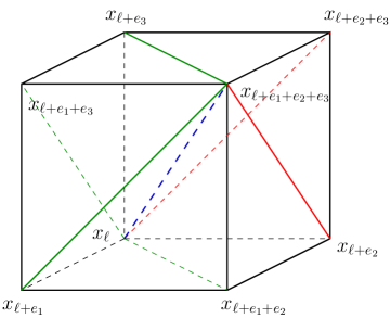
Figure 1. A type A decomposition of the cell $K_{\ell}$ into six tetrahedra.

Notice that in each tetrahedron originating from a type A decomposition of a cell, exactly three edges are edges of the original cell, these are depicted with solid, black lines in Fig. 2. To define the atomistic Cauchy–Born model on tetrahedra we need to define first discrete gradients at each tetrahedron $T.$ To this end, we assume that all cells are divided into tetrahedra from a type A decomposition. Let $v\in\boldsymbol{V}_{\varepsilon,T}$. Define $\widetilde{\nabla}v$ as

(2.3) $$\Big{\{}\widetilde{\nabla}v|_{T}\Big{\}}_{i\alpha}:=\widetilde{{D}}_{e_{\alpha}}v_{\ell}^{i},$$

where the discrete derivatives $\widetilde{{D}}_{e_{\alpha}}v_{\ell}^{i}$ on the tetrahedron $T$ are just the difference quotients of $v$ along the edges of $T$ with directions $e_{\alpha}$. These are the edges shared with those of $K_{\ell}$, shown in black solid lines in Fig. 2. For example, for the tetrahedron of Fig. 2, $\widetilde{{D}}_{e_{3}}v_{\ell}^{i}=\overline{D}_{e_{3}}v_{\ell}^{i}$, see (1.1), whereas $\widetilde{{D}}_{e_{2}}v_{\ell}^{i}=\overline{D}_{e_{2}}v_{\ell+e_{1}+e_{3}}^{i}$. Notice that the definition of these discrete derivatives can be extended to any smooth function. Then for each tetrahedron $T$ it follows that

$$\int_{T}W_{CB}(\nabla v)dx=\frac{\varepsilon^{3}}{6}W_{CB}(\widetilde{\nabla}v).$$

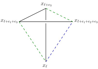
Figure 2. A typical tetrahedron resulting from the decomposition of the cell $K_{\ell}$. The three edges shown in solid, black lines are also edges of the original cell .

Further, let $y$ be a sufficiently smooth deformation. We define corresponding the atomistic Cauchy–Born (A–CB) energy

(2.4) $$\begin{split}\tilde{\Phi}^{a,CB}(y)&:=\frac{\varepsilon^{3}}{6}\sum_{\ell\in\mathfrak{L}}\ \,\sum_{T\in K_{\ell}(T)}\sum_{\eta\in R}\ \phi_{\eta}\,(\widetilde{\nabla}y\,\eta)=\frac{\varepsilon^{3}}{6}\sum_{\ell\in\mathfrak{L}}\,\sum_{T\in K_{\ell}(T)}W_{CB}(\widetilde{\nabla}y).\end{split}$$

Now, for a given field of external forces $f:\mathfrak{L}\to\mathbb{R}^{3}$ the tetrahedral A–CB problem reads as follows:

$$\begin{split}&\text{find a local minimizer $y^{a,CB}$ in $\mathcal{X}$ of : }\\ &\ \ \tilde{\Phi}^{a,CB}(y^{a,CB})-{\langle}f,y^{a,CB}{\rangle}_{\varepsilon}.\end{split}$$

If such a minimizer exists, then

$$\begin{split}{\langle}D\tilde{\Phi}^{a,CB}(y^{a,CB}),v{\rangle}_{\varepsilon}={\langle}f,v{\rangle}_{\varepsilon},\qquad\text{ for all }v\in{\mathscr{V}}.\end{split}$$

This atomistic model is consistent, in the sense that the above is satisfied for homogeneous deformations ($y_{F}(x)=\mathsf{F}x$, $x\in\Omega$):

(2.5) $${\langle}D\tilde{\Phi}^{a,CB}(y_{F}),v{\rangle}=0,\quad y_{F}(x)=\mathsf{F}x,$$

for all $v\in\boldsymbol{V}_{\varepsilon,T}.$ To show that, it suffices to observe

(2.6) $$\begin{split}{\langle}D\tilde{\Phi}^{a,CB}(y_{F}),v{\rangle}=&\frac{\varepsilon^{3}}{6}\sum_{\ell\in\mathfrak{L}}\ \,\sum_{T\in K_{\ell}(T)}\sum_{\eta\in R}\ \phi_{\eta}\,(\widetilde{\nabla}y_{F}\,\eta)\cdot\widetilde{\nabla}v\,\eta\\ =&\sum_{\eta\in R}\ \phi_{\eta}^{\prime}(F\,\eta)\cdot\sum_{\ell\in\mathfrak{L}}\ \,\frac{\varepsilon^{3}}{6}\sum_{T\in K_{\ell}(T)}\widetilde{\nabla}v\,\eta\\ =&\sum_{\eta\in R}\ \phi_{\eta}^{\prime}(F\,\eta)\cdot\sum_{\ell\in\mathfrak{L}}\ \,\sum_{T\in K_{\ell}(T)}\int_{T}{\nabla}v\,\eta\,dx\\ =&\sum_{\eta\in R}\ \phi_{\eta}^{\prime}(F\,\eta)\cdot\int_{\Omega}{\nabla}v\,\eta\,dx=0.\end{split}$$

An alternative discrete model defined over cells was introduced in [12]. The average discrete derivatives were defined, e.g., as

(2.7) $$\begin{split}\overline{\overline{D}}_{e_{1}}v_{\ell}=\frac{1}{4}\,\Big{\{}\overline{D}_{e_{1}}v_{\ell}+\overline{D}_{e_{1}}v_{\ell+e_{2}}+\overline{D}_{e_{1}}v_{\ell+e_{3}}+\overline{D}_{e_{1}}v_{\ell+e_{2}+e_{3}}\Big{\}}.\end{split}$$

This leads to a discrete gradient $\overline{\nabla}y$ in analogy to (2.3); see [12] for details. The corresponding cell atomistic Cauchy–Born energy is then defined by

$$\begin{split}{\Phi}^{a,CB}(y)&:={\varepsilon^{3}}\sum_{\ell\in\mathfrak{L}}\ \,\sum_{\eta\in R}\ \phi_{\eta}\,(\overline{\nabla}y\,\eta)={\varepsilon^{3}}\sum_{\ell\in\mathfrak{L}}\,W_{CB}(\overline{\nabla}y).\end{split}$$

The corresponding cell atomistic Cauchy–Born problem is

$$\begin{split}&\text{find a local minimizer $y^{a,CB}$ in $\mathcal{X}$ of : }\\ &\ \ {\Phi}^{a,CB}(y^{a,CB})-{\langle}f,y^{a,CB}{\rangle}_{\varepsilon}.\end{split}$$

This atomistic model is consistent as well, in the sense that

(2.8) $${\langle}D{\Phi}^{a,CB}(y_{F}),v{\rangle}=0,\quad y_{F}(x)=\mathsf{F}x\,,$$

for all $v\in\boldsymbol{V}_{\varepsilon,Q}.$ As before, this is implied by

(2.9) $$\begin{split}{\langle}D{\Phi}^{a,CB}(y_{F}),v{\rangle}=&{\varepsilon^{3}}\sum_{\ell\in\mathfrak{L}}\ \sum_{\eta\in R}\ \phi_{\eta}\,(\overline{\nabla}y_{F}\eta)\cdot\overline{\nabla}v\,\eta\\ =&\sum_{\eta\in R}\ \phi_{\eta}^{\prime}(F\,\eta)\cdot\sum_{\ell\in\mathfrak{L}}\ {\varepsilon^{3}}\,\overline{\nabla}v\,\eta\\ =&\sum_{\eta\in R}\ \phi_{\eta}^{\prime}(F\,\eta)\cdot\sum_{\ell\in\mathfrak{L}}\ \,\int_{K_{\ell}}{\nabla}v\,\eta\,dx\\ =&\sum_{\eta\in R}\ \phi_{\eta}^{\prime}(F\,\eta)\cdot\int_{\Omega}{\nabla}v\,\eta\,dx=0\,.\end{split}$$

It was shown in [12] that this model is both energy- and variationally consistent to second order in $\varepsilon,$ approximating the exact atomistic model as well as the continuum Cauchy-Born model.

3. Bond volumes and long range differences

To construct methods that couple the atomistic and continuum descriptions we need to relate long range differences and derivatives of functions defined over bond volumes. To fix ideas, let $\eta\in R,$ and define the bond as the line segment $b_{\ell}=\{x\in\mathbb{R}^{3}\colon{x=x_{\ell+t\eta}},\;0<t<1\}$ with endpoints $x_{\ell}$ and $x_{\ell+\eta}$. The set of all bonds $\mathcal{B}_{\eta}$ consists of all $b=b_{\ell}$ for $\ell\in\mathfrak{L}$ (but for $\eta$ fixed). For given $\ell$ and $\eta\in\mathbb{Z}^{3}$ with $\eta_{1}\eta_{2}\eta_{3}\neq 0,$ the corresponding bond volume $B_{\ell,\,\eta}$ is the interior of the rectangular parallelepiped with edges parallel to the standard basis vectors $e_{i}$ and main diagonal $b_{\ell}$, see Fig. 3. Next we shall establish a connection between long range differences and piecewise linear functions defined over type A decompositions of bond volumes $B_{\ell,\,\eta}$ into tetrahedra, which is defined in analogy to type A decompositions of cells $K_{\ell}.$ To this end let $B_{\ell,\,\eta}(T)$ a type A decomposition of the bond volume $B_{\ell,\,\eta}$ into six tetrahedra, i.e., the decomposition were the diagonals $(x_{\ell},x_{\ell+e_{1}\eta_{1}+e_{3}\eta_{3}})$ and $(x_{\ell+e_{2}\eta_{2}},x_{\ell+\eta})$ are edges of the resulting tetrahedra, see Fig. 3.

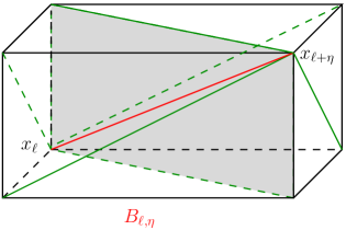
Figure 3. A bond volume $B_{\ell,\,\eta}$ and its type A decomposition into six tetrahedra.

The following lemma plays a central role in our work.

Lemma 3.1.

Let $v$ be a piecewise linear and continuous function on a type A decomposition of the bond volume $B_{\ell,\,\eta}$ into tetrahedra. Then

(3.1) $$\varepsilon^{3}\,\overline{D}_{\eta}v_{\ell}=\frac{1}{|\eta_{1}\,\eta_{2}\,\eta_{3}|}\,\int_{B_{\ell,\,\eta}}\,\nabla v(x)\eta\,dx\,.$$

Proof.

We present the proof for $\eta_{i}>0,$ $i=1,2,3$. The other cases are similar. We have,

(3.2) $$\begin{split}\frac{1}{\eta_{1}\,\eta_{2}\,\eta_{3}}\,\int_{B_{\ell,\,\eta}}\,\nabla v(x)\eta\,dx&=\frac{1}{\eta_{1}\,\eta_{2}\,\eta_{3}}\int_{\partial B_{\ell,\,\eta}}v\,\nu\cdot\eta\,ds\,\\ =\frac{1}{\eta_{1}\,\eta_{2}\,\eta_{3}}&\sum_{i=1}^{3}\Big{\{}\int_{\partial B_{\ell,\,\eta}(-e_{i})}\,(-\eta_{i})v\,ds+\int_{\partial B_{\ell,\,\eta}(e_{i})}\,\eta_{i}\,v\,ds\,\Big{\}}\,,\end{split}$$

where $\partial B_{\ell,\,\eta}(e_{i})$ is the face of $B_{\ell,\,\eta}$ with outward unit normal $e_{i}.$ Since $v$ is linear in each tetrahedron of the decomposition of $B_{\ell,\,\eta},$ it will be linear in each of the two triangles comprising the face $\partial B_{\ell,\,\eta}(\eta_{i}).$ Therefore, if $\tau$ is such a triangle, the integral of $v$ over $\tau$ can be found explicitly:

(3.3) $$\int_{\tau}\,\eta_{i}\,v\,ds=\frac{|\tau|}{3}\sum_{j=1}^{3}\ \eta_{i}\,v(z_{j}),$$

where $z_{i}$ are the vertices of $\tau$. Since $\tau$ is one of the two triangles of $\partial B_{\ell,\,\eta}(\eta_{i})$, ${|\tau|}\ \eta_{i}=\frac{\varepsilon^{2}}{2}\ \eta_{1}\,\eta_{2}\,\eta_{3}$. Hence,

(3.4) $$\frac{1}{\eta_{1}\,\eta_{2}\,\eta_{3}}\int_{\partial B_{\ell,\,\eta}(e_{i})}\,\eta_{i}\,v\,ds\,=\frac{\varepsilon^{2}}{6}\sum_{j=1}^{2}\ \big{\{}v(z_{j})+2\,v(\tilde{z}_{j})\big{\}},$$

where $\tilde{z}_{j}$ are the vertices shared by two triangles of $\partial B_{\ell,\,\eta}(e_{i})$ and $z_{j}$ the vertices belonging to only one triangle of $\partial B_{\ell,\,\eta}(e_{i})$.

We substitute the above formula into (3.2) and group together all terms involving each vertex. For each of the vertices other than $x_{\ell}$ or $x_{\ell+\eta}$, there are two possibilities:

1. It is a shared vertex in one face with outward normal $e_{i}$ and it is a single vertex in two faces with normal $-e_{i}$.

2. It is a shared vertex in one face with normal $-e_{i}$ and a single vertex in two faces with normal $e_{i}$.

Also, terms involving a vertex of $\partial B_{\ell,\,\eta}(e_{i})$ appear with coefficient $1$, while terms involving a vertex of $\partial B_{\ell,\,\eta}(-e_{i})$ appear with coefficient $-1$ in (3.2). Therefore the contribution of these vertices to the sum in (3.2) is zero.

Finally, we notice that $x_{\ell+\eta}$ is a shared vertex at each $\partial B_{\ell,\,\eta}(e_{i})$, while $x_{\ell}$ is a shared vertex at each $\partial B_{\ell,\,-\eta}(-e_{i})$, for all $i=1,2,3$. It follows that

(3.5) $$\begin{split}\frac{1}{\eta_{1}\,\eta_{2}\,\eta_{3}}\,\int_{B_{\ell,\,\eta}}\,\nabla v(x)\cdot\eta\,dx=\varepsilon^{2}\,\big{(}v_{\ell+\eta}-v_{\ell}\big{)},\end{split}$$

and the proof is complete. ∎

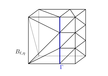
Figure 4. A possible decomposition ${\mathcal{T}}(B_{\ell,\,\eta})$ of $B_{\ell,\,\eta}.$

4. A coupling method based on bond volumes

In this section we construct methods based on bond volumes. Let the atomistic region $\Omega_{a}$ and the A-CB region $\Omega_{*}$ each be the interior of the closure of a union of lattice tetrahedra $T\in{\mathcal{T}}_{T}$ and connected, and suppose

$$\Omega=\overline{\Omega}_{a}\cup\overline{\Omega}_{*},\quad\Gamma=\overline{\Omega}_{a}\cap\overline{\Omega}_{*}.$$

Here $\Gamma$ is the interface. To avoid technicalities that may arise due to the fact that we work with periodic functions over $\Omega$, we assume throughout that $\overline{\Omega}_{a}$ is subset of the interior of $\Omega$ with sufficient distance from $\partial\Omega.$ Let $y_{\ell}$ be the deformed position of $x_{\ell}\in\Omega_{\text{discr}}$.

Fix $\eta\in R,$ with $\eta_{1}\eta_{2}\eta_{3}\neq 0.$ The cases of degenerate $\eta$ can be treated with two and one dimensional techniques. We shall construct an energy based coupling method whose design relies on an appropriate handling of bond volumes $B_{\ell,\,\eta}$. We consider three cases depending on the location of each bond volume $B_{\ell,\,\eta}$:

1. The closure of the bond volume is contained in the atomistic region: $\overline{B}_{\ell,\,\eta}\subset\Omega_{a}$.

2. The bond volume is contained in the region $\Omega_{*}$: $B_{\ell,\,\eta}\subset\Omega_{*}$.

3. We denote by $B_{\Gamma}$ the set of bond volumes that do not satisfy (a) or (b). In fact, $B_{\ell,\,\eta}\in B_{\Gamma}$ if the bond volume intersects the interface: $B_{\ell,\,\eta}\cap\Gamma\neq\emptyset$ or if $B_{\ell,\,\eta}\subset\Omega_{a}$ and $\overline{B}_{\ell,\,\eta}\cap\Gamma\neq\emptyset$.

If a bond volume intersects $\partial\Omega,$ then it is supposed to belong to $\Omega_{*}$ by periodic extension. For a fixed $\eta,$ the contribution to the energy corresponding to the atomistic region (case (a)) is

(4.1) $$E_{\Omega_{a},\eta}^{a}\{y\}=\varepsilon^{3}\sum_{\begin{subarray}{c}\ell\in\mathfrak{L}\\ \overline{B}_{\ell,\,\eta}\subset\Omega_{a}\end{subarray}}\phi_{\eta}(\overline{D}_{\eta}y_{\ell})\,.$$

The contribution to the energy from the A-CB region (case (b)) is (cf. (2.4)),

(4.2) $$E_{\Omega_{*},\eta}^{a,cb}\{y\}=\frac{\varepsilon^{3}}{6}\,\sum_{\ell\in\mathfrak{L},\ T\in K_{\ell}(T),\ T\subset\Omega_{*}}\ \phi_{\eta}\,(\widetilde{\nabla}y\,\eta)=\int_{\Omega_{*}}\phi_{\eta}({\nabla}\overline{y}(x)\eta)dx\,,$$

$\overline{y}$ being the interpolant of $\{y_{\ell}\}$ in $\boldsymbol{V}_{\varepsilon,T}(\Omega_{*})$, see below (2.2).

For each bond volume intersecting $\Gamma$ we denote by $y^{\ell,\eta}$ a piecewise polynomial function on $B_{\ell,\,\eta}$ satisfying

1. $y^{\ell,\eta}\in C(\overline{B}_{\ell,\,\eta})$.

2. Let ${\mathcal{T}}(B_{\ell,\,\eta})$ be a decomposition of $B_{\ell,\,\eta}$ with the following properties: a) if $T\in{\mathcal{T}}(B_{\ell,\,\eta})$ and $T\subset\Omega_{*}$ then $T$ is a tetrahedron resulting from a type A decomposition of an atomistic cell $K\subset\Omega_{*}$. b) If $T\in{\mathcal{T}}(B_{\ell,\,\eta})$ and $T\subset\Omega_{a}$, then $T$ is a lattice tetrahedron.

3. In case ii.b) above, if $T$ has a face on $\partial\big{(}B_{\ell,\,\eta}\cap\Omega_{a}\big{)}\backslash\Gamma$, then it is part of a conforming decomposition that is compatible with decompositions of other bond volumes sharing a face with $B_{\ell,\eta}$. If such an attached bond volume is included in $\Omega_{a}$, then it is assumed to be type-A decomposed into tetrahedra.

4. For $T\in{\mathcal{T}}(B_{\ell,\,\eta}),$ $y^{\ell,\eta}\in\mathbb{P}_{1}(T)$ and it interpolates $\{y_{\ell}\}$ at the vertices of $T$.

Then the energy due to bond volumes intersecting the interface is defined as

(4.3) $$E_{\Gamma,\eta}\{y\}=\sum_{\begin{subarray}{c}\ell\in\mathfrak{L}\\ B_{\ell,\,\eta}\in B_{\Gamma}\end{subarray}}\frac{1}{|\eta_{1}\,\eta_{2}\,\eta_{3}|}\int_{B_{\ell,\,\eta}}\chi_{{}_{\Omega_{a}}}\phi_{\eta}(\nabla y^{\ell,\eta}\eta)\,dx\,.$$

Remark 4.1.

Notice that the energy that corresponds to the bond volume $B_{\ell,\,\eta}\in B_{\Gamma}$ would be

(4.4) $$\frac{1}{|\eta_{1}\,\eta_{2}\,\eta_{3}|}\int_{B_{\ell,\,\eta}}\phi_{\eta}(\nabla y^{\ell,\eta}\eta)\,dx\,.$$

The part of this energy corresponding to $B_{\ell,\,\eta}\cap\Omega_{*}$ has been already taken into account in $E_{\Omega_{*},\eta}^{a,cb}\{y\}$ and hence it is not included in the definition of $E_{\Gamma,\eta}\{y\}\,.$

Remark 4.2.

The choice of the decomposition ${\mathcal{T}}(B_{\ell,\,\eta})$ and of the associated piecewise polynomial function $y^{\ell,\eta}$ is somewhat flexible; see [11] for a more detailed discussion. It might even allow vertices that are not lattice points. The only essential requirement is that each function $v^{[m]}$ defined through ${\mathcal{T}}(B_{\ell,\,\eta})$ in the proof of Proposition 4.1 below, should satisfy $v^{[m]}\in H^{1}(\Omega)\,.$ Depending on the complexity of the interface $\Gamma$ one can construct such decompositions more or less efficiently. In many cases this can simplify the computation of the associated energy $E_{\Gamma,\eta}\{y\}$. See for example, Figure 4 for such a choice of decomposition.

We then define the total energy as follows

(4.5) $$\mathcal{E}_{bv}\{y\}=\sum_{\eta\in R}\mathcal{E}_{\,\eta}\{y\}$$

where

(4.6) $$\mathcal{E}_{\,\eta}\{y\}=E_{\Omega_{a},\eta}^{a}\{y\}+E_{\Omega_{*},\eta}^{a,cb}\{y\}+E_{\Gamma,\eta}\{y\}\,.$$

4.1. Consistency

The energy (4.5) based on bond volumes is ghost-force free, as we prove in the following proposition.

Proposition 4.1.

The energy (4.5) is free of ghost forces, in the sense that

(4.7) $${\langle}D\mathcal{E}_{bv}(y_{F}),v{\rangle}=0,\quad y_{F}(x)=\mathsf{F}x\,,$$

for all $v\in{\mathscr{V}}$.

To show this proposition we shall need some more notation. First we fix $\eta$ and consider decompositions into bond volumes which cover $\mathbb{R}^{3}$:

(4.8) $$\begin{split}&\mathcal{S}^{m}_{B_{\eta}}:=\Big{\{}B_{\ell,\,\eta}\,:\ \text{(i)}\ B_{\ell,\,\eta}\cap B_{j,\,\eta}=\emptyset,\text{ if }\ell\neq j,\quad\text{(ii)}\ \mathbb{R}^{2}=\overline{\cup B_{\ell,\,\eta}}\ \Big{\}}\,,\quad m=1,\dots,|\eta_{1}\,\eta_{2}\,\eta_{3}|.\end{split}$$

$\mathcal{S}^{m}_{B_{\eta}}$ will be used for counting purposes in the proof; the associated functions introduced below will be defined on $\Omega.$ The number of different such coverings is $|\eta_{1}\,\eta_{2}\,\eta_{3}|\,,$ hence the numbering $m=1,\dots,|\eta_{1}\,\eta_{2}\,\eta_{3}|.$ Notice that bond volumes corresponding to different $m$ may overlap, but the elements of a single $\mathcal{S}^{m}_{B_{\eta}}$ are non-overlapping bond volumes.

For a lattice function $\{v_{\ell}\}$ construct the functions ${\nabla}\overline{v}$ and $v^{\ell,\eta}$ in analogy with ${\nabla}\overline{y}$ and $y^{\ell,\eta}$ in the construction below (4.2). Then for a fixed $\eta$ we have

(4.9) $$\begin{split}{\langle}D\mathcal{E}_{\,\eta}(y_{F}),v{\rangle}=\phi_{\eta}^{\prime}(F\,\eta)\cdot\Big{\{}&\varepsilon^{3}\sum_{\begin{subarray}{c}\ell\in\mathfrak{L}\\ \overline{B}_{\ell,\,\eta}\subset\Omega_{a}\end{subarray}}\,\overline{D}_{\eta}v_{\ell}+\int_{\Omega_{*}}{\nabla}\overline{v}(x)\eta\,dx\\ \ &+\sum_{\begin{subarray}{c}\ell\in\mathfrak{L}\\ B_{\ell,\,\eta}\in B_{\Gamma}\end{subarray}}\frac{1}{|\eta_{1}\,\eta_{2}\,\eta_{3}|}\int_{B_{\ell,\,\eta}}\chi_{{}_{\Omega_{a}}}\nabla v^{\ell,\eta}\eta\,dx\Big{\}}\,.\end{split}$$

The main idea in the proof of Proposition 4.1 is to rewrite the expression within brackets above in the following way:

(4.10) $$\begin{split}\varepsilon^{3}\sum_{\begin{subarray}{c}\ell\in\mathfrak{L}\\ \overline{B}_{\ell,\,\eta}\subset\Omega_{a}\end{subarray}}\,\overline{D}_{\eta}v_{\ell}&+\int_{\Omega_{*}}\overline{\nabla}v(x)\eta\,dx\ +\sum_{\begin{subarray}{c}\ell\in\mathfrak{L}\\ B_{\ell,\,\eta}\in B_{\Gamma}\end{subarray}}\frac{1}{|\eta_{1}\,\eta_{2}\,\eta_{3}|}\int_{B_{\ell,\,\eta}}\chi_{{}_{\Omega_{a}}}\nabla v^{\ell,\eta}\eta\,dx\\ &=\frac{1}{|\eta_{1}\,\eta_{2}\,\eta_{3}|}\sum_{m=1}^{|\eta_{1}\,\eta_{2}\,\eta_{3}|}\,\int_{\Omega}{\nabla}v^{[m]}(x)\eta\,dx,\end{split}$$

where $v^{[m]},$ $m=1,\dots,|\eta_{1}\,\eta_{2}\,\eta_{3}|$ are appropriate conforming functions in $H^{1}(\Omega)$, each associated to a different covering $\mathcal{S}^{m}_{B_{\eta}}$ consisting of bond volumes. The details are provided below.

Proof of Proposition 4.1. We use Lemma 3.1 to write

(4.11) $$\begin{split}\varepsilon^{3}\sum_{\begin{subarray}{c}\ell\in\mathfrak{L}\\ \overline{B}_{\ell,\,\eta}\subset\Omega_{a}\end{subarray}}\,\overline{D}_{\eta}v_{\ell}=\frac{1}{|\eta_{1}\,\eta_{2}\,\eta_{3}|}\sum_{\begin{subarray}{c}\ell\in\mathfrak{L}\\ \overline{B}_{\ell,\,\eta}\subset\Omega_{a}\end{subarray}}\,\int_{B_{\ell,\,\eta}}\,\nabla v^{[m]}(x)\eta\,dx\end{split}$$

where $v^{[m]}$ is a piecewise linear continuous function on a type A decomposition of the bond volume $B_{\ell,\,\eta}$ into tetrahedra. The superscript $m$ indicates the covering $\mathcal{S}^{m}_{B_{\eta}}$ to which $B_{\ell,\,\eta}$ belongs. In fact, $v^{[m]}$ can be defined globally as follows: For a given lattice function $\{v_{\ell}\},$ a fixed $m$ and a covering $\mathcal{S}^{m}_{B_{\eta}}$ $v^{[m]}$ is equal to

1. the piecewise linear interpolant of $\{v_{\ell}\}$ on a type A decomposition of the bond volume $B_{\ell,\,\eta}$ into tetrahedra if $\overline{B}_{\ell,\,\eta}\subset\Omega_{a},$

2. $v^{\ell,\eta},$ for $B_{\ell,\,\eta}\cap\Gamma\neq\emptyset,$ where the piecewise polynomial $v^{\ell,\eta}$ on $B_{\ell,\,\eta}$ is defined through (i–iv) below (4.2),

3. the piecewise linear function interpolating $\{v_{\ell}\}$ at lattice tetrahedra $T\subset B_{\ell,\,\eta}\subset\Omega_{*}.$

It is clear by construction that each $v^{[m]}\in H^{1}(\Omega)\,.$ Further, each tetrahedron corresponds to exactly one atomistic cell $K\subset\Omega_{*}$ belonging to $|\eta_{1}\eta_{2}\eta_{3}|$ different bond volumes $B_{\ell,\,\eta}$, each one belonging to a different covering $\mathcal{S}^{m}_{B_{\eta}}.$ Thus for $T\subset\Omega_{*}$ we have

(4.12) $$\int_{T}{\nabla}\overline{v}(x)\eta\,dx=\frac{1}{|\eta_{1}\,\eta_{2}\,\eta_{3}|}\sum_{m=1}^{|\eta_{1}\,\eta_{2}\,\eta_{3}|}\int_{T\cap B_{\ell,\,\eta}\in\mathcal{S}^{m}_{B_{\eta}}}\nabla v^{[m]}(x)\eta\,dx\,.$$

Therefore,

(4.13) $$\begin{split}\int_{\Omega_{*}}{\nabla}\overline{v}(x)\eta\,dx=\frac{1}{|\eta_{1}\,\eta_{2}\,\eta_{3}|}\sum_{m=1}^{|\eta_{1}\,\eta_{2}\,\eta_{3}|}\int_{\Omega_{*}}\nabla v^{[m]}(x)\eta\,dx\,.\end{split}$$

By construction of $v^{\ell,\eta}$ and $v^{[m]}$ we have

(4.14) $$\sum_{\begin{subarray}{c}\ell\in\mathfrak{L}\\ B_{\ell,\,\eta}\in B_{\Gamma}\end{subarray}}\frac{1}{|\eta_{1}\,\eta_{2}\,\eta_{3}|}\int_{B_{\ell,\,\eta}}\chi_{{}_{\Omega_{a}}}\nabla v^{\ell,\eta}\eta\,dx=\frac{1}{|\eta_{1}\,\eta_{2}\,\eta_{3}|}\sum_{m=1}^{|\eta_{1}\,\eta_{2}\,\eta_{3}|}\ \sum_{\begin{subarray}{c}B_{\ell,\,\eta}\in\mathcal{S}^{m}_{B_{\eta}}\\ B_{\ell,\,\eta}\in B_{\Gamma}\end{subarray}}\ \int_{B_{\ell,\,\eta}}\chi_{{}_{\Omega_{a}}}\nabla v^{[m]}(x)\eta\,dx$$

Thus rewriting (4.11) as

(4.15) $$\begin{split}\varepsilon^{3}\sum_{\begin{subarray}{c}\ell\in\mathfrak{L}\\ \overline{B}_{\ell,\,\eta}\subset\Omega_{a}\end{subarray}}\,\overline{D}_{\eta}v_{\ell}=\frac{1}{|\eta_{1}\,\eta_{2}\,\eta_{3}|}\sum_{m=1}^{|\eta_{1}\,\eta_{2}\,\eta_{3}|}\ \sum_{\begin{subarray}{c}B_{\ell,\,\eta}\in\mathcal{S}^{m}_{B_{\eta}}\\ \overline{B}_{\ell,\,\eta}\subset\Omega_{a}\end{subarray}}\ \int_{B_{\ell,\,\eta}}\nabla v^{[m]}(x)\eta\,dx,\end{split}$$

we finally obtain

(4.16) $$\begin{split}\varepsilon^{3}\sum_{\begin{subarray}{c}\ell\in\mathfrak{L}\\ \overline{B}_{\ell,\,\eta}\subset\Omega_{a}\end{subarray}}\,\overline{D}_{\eta}v_{\ell}&+\sum_{\begin{subarray}{c}\ell\in\mathfrak{L}\\ B_{\ell,\,\eta}\in B_{\Gamma}\end{subarray}}\frac{1}{|\eta_{1}\,\eta_{2}\,\eta_{3}|}\int_{B_{\ell,\,\eta}}\chi_{{}_{\Omega_{a}}}\nabla v^{\ell,\eta}\eta\,dx\\ &=\frac{1}{|\eta_{1}\,\eta_{2}\,\eta_{3}|}\sum_{m=1}^{|\eta_{1}\,\eta_{2}\,\eta_{3}|}\ \sum_{\begin{subarray}{c}B_{\ell,\,\eta}\in\mathcal{S}^{m}_{B_{\eta}}\\ B_{\ell,\,\eta}\in B_{\Gamma}\ \text{ or }\ \overline{B}_{\ell,\,\eta}\subset\Omega_{a}\end{subarray}}\ \int_{B_{\ell,\,\eta}}\chi_{{}_{\Omega_{a}}}\nabla v^{[m]}(x)\eta\,dx\\ &=\frac{1}{|\eta_{1}\,\eta_{2}\,\eta_{3}|}\sum_{m=1}^{|\eta_{1}\,\eta_{2}\,\eta_{3}|}\ \int_{\Omega_{a}}\nabla v^{[m]}(x)\eta\,dx\,.\end{split}$$

Hence (4.10) follows in view of (4.12). Therefore the proof of proposition is complete in view of the Gauss-Green theorem. ∎

5. The discontinuous bond volume based coupling method

In this section we show that is is possible to modify energies to allow underlying functions which might be discontinuous at the interface. This allows greater flexibility on the construction of the underlying meshes and thus the computation of the energy at the interface might become simpler. To retain consistency the interfacial energies should include terms accounting for the possible discontinuity of the underlying functions. There are many alternatives, such as the possibility of adding extra stabilization terms, compare to [1]. The purpose of this paper is however to present the general framework and we will not insist on the various modifications and extensions of the methods developed herein.

Let $\Omega$, $\Omega_{a},$ $\Omega_{*}$ and $\Gamma$ be as in the previous section. Further, we distinguish the same cases a), b) and c) regarding the location of each bond volume $B_{\ell,\,\eta}.$ The corresponding energies are still defined by

(5.1) $$E_{\Omega_{a},\eta}^{a}\{y\}=\varepsilon^{3}\sum_{\begin{subarray}{c}\ell\in\mathfrak{L}\\ \overline{B}_{\ell,\,\eta}\subset\Omega_{a}\end{subarray}}\phi_{\eta}(\overline{D}_{\eta}y_{\ell}),$$

and

(5.2) $$E_{\Omega_{*},\eta}^{a,cb}\{y\}=\frac{\varepsilon^{3}}{6}\,\sum_{\ell\in\mathfrak{L},\ T\in K_{\ell}(T),\ T\subset\Omega_{*}}\ \phi_{\eta}\,(\widetilde{\nabla}y\,\eta)=\int_{\Omega_{*}}\phi_{\eta}({\nabla}\overline{y}(x)\eta)dx\,,$$

$\overline{y}$ being the piecewise linear function at the lattice tetrahedra interpolating $\{y_{\ell}\}$. The main difference to the previous construction in Section 3 is the choice of $y^{\ell,\eta}$ and the corresponding energies for each bond volume intersecting the interface. In fact we let

1. $y^{\ell,\eta}\in C(\overline{B_{\ell,\,\eta}}\ \backslash\Gamma).$

2. Further, let ${\mathcal{T}}(B_{\ell,\,\eta})$ be a decomposition of $B_{\ell,\,\eta}$ with the properties a) if ${T}\in{\mathcal{T}}(B_{\ell,\,\eta})$ and ${T}\subset\Omega_{*}$ then ${T}$ is an atomistic tetrahedron resulting from a type A decomposition of an atomistic cell. b) If ${T}\in{\mathcal{T}}(B_{\ell,\,\eta})$ and ${T}\subset\Omega_{a}$ then ${T}$ is a lattice tetrahedron.

3. In the case ii.b) above if ${T}$ has a face on $\partial\big{(}B_{\ell,\,\eta}\cap\Omega_{a}\big{)}\backslash\Gamma$ then it will allow for a compatible conforming decomposition with respect to attached bond volumes. In that case if the attached bond volume is included in $\Omega_{a}$ it is assumed to be type-A decomposed into tetrahedra.

4. For ${T}\in{\mathcal{T}}(B_{\ell,\,\eta}),$ $y^{\ell,\eta}\in\mathbb{P}_{1}({T}),$ interpolating $\{y_{\ell}\}\,$ at the vertices of ${T}$.

We have kept the same properties, but we allow discontinuous matching across the interface $\Gamma.$ This provides greater flexibility on the construction of $y^{\ell,\eta}$ since it allows the presence of arbitrary hanging nodes on the interface of the two regions.

We then define the energy due to bond volumes intersecting the interface as

(5.3) $$E_{\Gamma,\eta}^{D}\{y\}=\sum_{\begin{subarray}{c}\ell\in\mathfrak{L}\\ B_{\ell,\,\eta}\in B_{\Gamma}\end{subarray}}\frac{1}{|\eta_{1}\eta_{2}\eta_{3}|}\Big{[}\int_{B_{\ell,\,\eta}}\chi_{{}_{\Omega_{a}}}\phi_{\eta}(\nabla y^{\ell,\eta}\eta)\,dx-\int_{B_{\ell,\,\eta}\cap\Gamma}\phi_{\eta}^{\prime}({\{\!\!\{\nabla y^{\ell,\eta}\eta\}\!\!\}})\,{\cdot}{[\![y^{\ell,\eta}\eta]\!]}\,dS\,\Big{]}.$$

Here, ${[\![w\eta]\!]}$, ${\{\!\!\{w\}\!\!\}}$ denote the jump and the average of a possibly discontinuous function on the interface

(5.4) $${{[\![w\eta]\!]}:=(\nu_{\Omega_{a}}\cdot\eta)\,w^{-}\,+(\nu_{\Omega_{*}}\cdot\eta)\,w^{+}},\qquad{\{\!\!\{w\}\!\!\}}:=\frac{1}{2}\{w^{-}\,+w^{+}\}\,,$$

where $w^{-}$ and $w^{+}$ being the limits taken from $\Omega_{a}$ and $\Omega_{*}$ respectively, and $\nu_{\Omega_{a}}$, $\nu_{\Omega_{*}}$ the corresponding exterior normal unit vectors, with $\nu_{\Omega_{a}}=-\nu_{\Omega_{*}}$ on $\Gamma$.

A key observation here is that $E_{\Gamma,\eta}^{D}\{y\}$ does not induce inconsistencies on the energy level. In fact, it is obvious that if $y^{\ell,\eta}\in C(\overline{B_{\ell,\,\eta}})$ as in the previous section, then

(5.5) $$E_{\Gamma,\eta}^{D}\{y\}=E_{\Gamma,\eta}\{y\}\,,$$

since the extra term on the interface vanishes. Then, as in the previous section, we define the total energy as follows:

(5.6) $$\mathcal{E}_{bv}^{D}\{y\}=\sum_{\eta\in R}\mathcal{E}^{D}_{\,\eta}\{y\},$$

where

(5.7) $$\mathcal{E}^{D}_{\,\eta}\{y\}=E_{\Omega_{a},\eta}^{a}\{y\}+E_{\Omega_{*},\eta}^{a,cb}\{y\}+E_{\Gamma,\eta}^{D}\{y\}\,.$$

Despite the fact that we allow discontinuities, the energy $\mathcal{E}_{bv}^{D}$ is still ghost-force free:

Proposition 5.1.

The energy (5.6) is free of ghost forces, in the sense that

(5.8) $${\langle}D\mathcal{E}_{bv}^{D}(y_{F}),v{\rangle}=0,\quad y_{F}(x)=\mathsf{F}x,$$

for all $v\in{\mathscr{V}}$.

Proof.

The structure of the proof is the same to that of Proposition 4.1, hence we present in detail only the main differences. We still need the coverings $\mathcal{S}^{m}_{B_{\eta}}$ and recall that their elements define a decomposition of non-overlapping bond volumes. As in the proof of Proposition 4.1 for a given lattice function $\{v_{\ell}\}$ we define the functions ${\nabla}\overline{v}$ and $v^{\ell,\eta}$ in analogy with ${\nabla}\overline{y}$ and $y^{\ell,\eta},$ cf., (4.2). Then, we have

(5.9) $$\begin{split}{\langle}D\mathcal{E}^{D}_{\,\eta}(y_{F}),v{\rangle}=\phi_{\eta}^{\prime}(F\,\eta)\cdot\Big{\{}&\varepsilon^{3}\sum_{\begin{subarray}{c}\ell\in\mathfrak{L}\\ \overline{B}_{\ell,\,\eta}\subset\Omega_{a}\end{subarray}}\,\overline{D}_{\eta}v_{\ell}+\int_{\Omega_{*}}{\nabla}\overline{v}(x)\eta\,dx\\ \ &+\frac{1}{|\eta_{1}\,\eta_{2}\,\eta_{3}|}\sum_{\begin{subarray}{c}\ell\in\mathfrak{L}\\ B_{\ell,\,\eta}\in B_{\Gamma}\end{subarray}}\int_{B_{\ell,\,\eta}}\chi_{{}_{\Omega_{a}}}\nabla v^{\ell,\eta}\eta\,dx-\int_{B_{\ell,\,\eta}\cap\Gamma}{[\![v^{\ell,\eta}\eta]\!]}\,dS\,\Big{\}}\,.\end{split}$$

Indeed, to show this it suffices to evaluate

(5.10) $${\langle}D\big{[}\phi_{\eta}^{\prime}({\{\!\!\{\nabla w\eta\}\!\!\}}){\cdot}{[\![w\eta]\!]}\,\big{]},v{\rangle}={\Bigl{(}}\phi_{\eta}^{\prime\prime}({\{\!\!\{\nabla w\eta\}\!\!\}})\,{[\![w\eta]\!]}{\Bigl{)}\cdot}{\{\!\!\{\nabla v\eta\}\!\!\}}+\phi_{\eta}^{\prime}({\{\!\!\{\nabla w\eta\}\!\!\}}){\cdot}{[\![v\eta]\!]},$$

which is equal to ${\phi_{\eta}^{\prime}(F\eta)\cdot{[\![v\eta]\!]}}$ for $w=y_{F}$.

In parallel to the proof of Proposition 4.1 we shall prove

(5.11) $$\begin{split}\varepsilon^{3}\!\!\!\sum_{\begin{subarray}{c}\ell\in\mathfrak{L}\\ \overline{B}_{\ell,\,\eta}\subset\Omega_{a}\end{subarray}}\,\overline{D}_{\eta}v_{\ell}&+\int_{\Omega_{*}}\overline{\nabla}v(x)\eta\,dx\ +\!\!\!\!\sum_{\begin{subarray}{c}\ell\in\mathfrak{L}\\ B_{\ell,\,\eta}\in B_{\Gamma}\end{subarray}}\frac{1}{|\eta_{1}\,\eta_{2}\,\eta_{3}|}\,\Big{[}\int_{B_{\ell,\,\eta}}\chi_{{}_{\Omega_{a}}}\nabla v^{\ell,\eta}\eta\,dx-\int_{B_{\ell,\,\eta}\cap\Gamma}{[\![v^{\ell,\eta}\eta]\!]}\,dS\,\Big{]}\\ &=\frac{1}{|\eta_{1}\,\eta_{2}\,\eta_{3}|}\sum_{m=1}^{|\eta_{1}\,\eta_{2}\,\eta_{3}|}\,\ \Big{[}\int_{\Omega\backslash\Gamma}{\nabla}v^{[m]}(x)\eta\,dx-\int_{\Gamma}{[\![v^{[m]}\eta]\!]}\,dS\,\Big{]}\\ \ \end{split}$$

where $v^{[m]},$ $m=1,\dots,|\eta_{1}\,\eta_{2}\,\eta_{3}|$, are appropriate functions in $H^{1}(\Omega\backslash\Gamma)\cap C(\overline{\Omega}\backslash\Gamma),$ possibly discontinuous at $\Gamma;$ each $v^{[m]}$ is associated to a different covering $\mathcal{S}^{m}_{B_{\eta}}$ consisting of bond volumes. Relation (5.11) then implies ${\langle}D\mathcal{E}^{D}_{\,\eta}(y_{F}),v{\rangle}=0$ since by the Gauss Green theorem,

$$\int_{\Omega\backslash\Gamma}{\nabla}v^{[m]}(x)\eta\,dx=\int_{\Gamma}{[\![v^{[m]}\eta]\!]}\,dS\,.$$

It remains therefore to establish (5.11). To this end, we proceed exactly as in the proof of Proposition 4.1. In particular, for a given lattice function $\{v_{\ell}\}$, a fixed $m$ and a covering $\mathcal{S}^{m}_{B_{\eta}}$ define $v^{[m]}$ as

1. the piecewise linear interpolant of $\{v_{\ell}\}$ on a type A decomposition of the bond volume $B_{\ell,\,\eta}$ into tetrahedra if $\overline{B}_{\ell,\,\eta}\subset\Omega_{a},$

2. $v^{\ell,\eta},$ for $B_{\ell,\,\eta}\cap\Gamma\neq\emptyset,$ where the piecewise polynomial on $B_{\ell,\,\eta},$ $v^{\ell,\eta}$ is possibly discontinuous on $B_{\ell,\,\eta}\cap\Gamma,$ and is defined through (i–iv) above,

3. the piecewise linear function at the lattice tetrahedra interpolating $\{v_{\ell}\}$, if $T$ is an atomistic tetrahedron such that ${T}\subset B_{\ell,\,\eta}\subset\Omega_{*}$.

Now, by construction $v^{[m]}\in H^{1}(\Omega\backslash\Gamma)\cap C(\overline{\Omega}\backslash\Gamma)$, and is possibly discontinuous at $\Gamma$. The rest of the proof is identical to the one of Proposition 4.1 with the exception that (4.14) should be replaced by

(5.12) $$\begin{split}\sum_{\begin{subarray}{c}\ell\in\mathfrak{L}\\ B_{\ell,\,\eta}\in B_{\Gamma}\end{subarray}}\frac{1}{|\eta_{1}\,\eta_{2}\,\eta_{3}|}&\int_{B_{\ell,\,\eta}}\chi_{{}_{\Omega_{a}}}\nabla v^{\ell,\eta}\eta\,dx-\int_{B_{\ell,\,\eta}\cap\Gamma}{[\![v^{\ell,\eta}\eta]\!]}\,dS\\ &=\frac{1}{|\eta_{1}\,\eta_{2}\,\eta_{3}|}\sum_{m=1}^{|\eta_{1}\,\eta_{2}\,\eta_{3}|}\ \sum_{\begin{subarray}{c}B_{\ell,\,\eta}\in\mathcal{S}^{m}_{B_{\eta}}\\ B_{\ell,\,\eta}\in B_{\Gamma}\end{subarray}}\ \int_{B_{\ell,\,\eta}}\chi_{{}_{\Omega_{a}}}\nabla v^{[m]}(x)\eta\,dx-\int_{B_{\ell,\,\eta}\cap\Gamma}{[\![v^{[m]}\eta]\!]}\,dS,\end{split}$$

with (4.16) modified accordingly. ∎

6. High-order finite element coupling

In this section we shall see how the previous analysis can lead to energy-based methods which employ high-order (even $hp$-) finite element approximations of the Cauchy-Born energy on the continuum region while remaining ghost-force free. To this end let ${\mathcal{T}}_{ac}$ be a decomposition of $\Omega$ into elements with the following properties: Let $\Omega$, $\Omega_{a}$ and $\Omega_{*}$ as before with $\Gamma$ the interface. The approximations will be based on decompositions of the continuum region $\Omega_{*}$ that are compatible on $\Gamma$ to $\boldsymbol{V}_{\varepsilon,T}(\Omega_{*}).$ To this end, let

(6.1) $$\begin{split}{\mathcal{T}}_{c}(\Omega_{*})\quad&\text{be a conforming decomposition of }\ \Omega_{*}\ \text{ into tetrahedra with vertices lattice points,}\\ &\text{such that, if }\ T\in{\mathcal{T}}_{c}(\Omega_{*}),\overline{T}\cap\Gamma\neq\emptyset,\quad\text{then}\quad T\in{\mathcal{T}}_{T}(\Omega_{*})\,.\end{split}$$

We consider the discrete space

(6.2) $$\begin{split}\boldsymbol{V}_{h,ac}(\Omega_{*})=\{v\in C(\overline{\Omega}_{*}):&\ v|_{T}\in\mathbb{P}_{1}(T)\ \text{for }\overline{T}\cap\Gamma\neq\emptyset\text{ and }\\ &\ v|_{T}\in\mathbb{P}_{k}(T)\ \text{for all other }T\in{\mathcal{T}}_{c}(\Omega_{*})\,\}\,.\end{split}$$

This space can be extended to include the atomistic region as well by

(6.3) $$\begin{split}\boldsymbol{V}_{h,ac}=\{v\in C(\overline{\Omega}):&\ v|_{T}\in\mathbb{P}_{1}(T)\ \text{for }T\in{\mathcal{T}}_{T}(\Omega_{a})\text{ and }\\ &v|_{T}\in\boldsymbol{V}_{h,ac}(\Omega_{*})\ \text{for all }T\in{\mathcal{T}}_{c}(\Omega_{*}),\ \ v\ \text{periodic on }\Omega\,\}\,.\end{split}$$

For $v\in\boldsymbol{V}_{h,ac}$ one can define the corresponding lattice function $\{v_{\ell}\}$, simply by interpolating. Conversely, for given $\{v_{\ell}\}$ one can find $v\in\boldsymbol{V}_{h,ac}$ that coincides with corresponding values of $\{v_{\ell}\}$ at the vertices. However, at the regions using high-order finite elements the other degrees of freedom should be defined with some care. In the following, we assume that we are given a function $y,$ $y(x)=\mathsf{F}x+v(x),$ $v\in\boldsymbol{V}_{h,ac}$ and we shall define its atomistic/continuum energy. To this end,

(6.4) $$\mathcal{E}_{\,h}=\sum_{\eta\in R}\ \mathcal{E}_{\,h,\eta}\,,$$

where

(6.5) $$\mathcal{E}_{\,h,\eta}\{y\}=E_{\Omega_{a},\eta}^{a}\{y\}+\int_{\Omega_{*}}\phi_{\eta}({\nabla}y(x)\eta)dx+E_{\Gamma,\eta}\{y\}\,.$$

Here for an atomistic point $x_{\ell}\in\Omega_{a},$ $y_{\ell}=y(x_{\ell}),$ and the local energies $E_{\Omega_{a},\eta}^{a}\{y\},$ $E_{\Gamma,\eta}\{y\}$ are defined as in Section 4, see (4.1), (4.3).

The above method can designed to be of arbitrary high order accuracy of the Cauchy-Born energy at the continuum region $\Omega_{*}\,.$ Such methods are of importance since, by tuning the discretization parameters (decomposition of $\Omega_{*}\,$ and polynomial degrees) we have the possibility of matching the ideal accuracy at the continuum region which is $O(\varepsilon^{2}).$ The energy $\mathcal{E}_{\,h}$ is ghost force free.

Proposition 6.1.

The energy (6.4) is free of ghost forces, in the sense that

(6.6) $${\langle}D\mathcal{E}_{\,h}(y_{F}),v{\rangle}=0,\quad y_{F}(x)=\mathsf{F}x\,,$$

for all $v\in\boldsymbol{V}_{h,ac}\,.$

Proof.

Since $v\in\boldsymbol{V}_{h,ac}$ we have

(6.7) $$\begin{split}{\langle}D\mathcal{E}_{\,h,\eta}(y_{F}),v{\rangle}=\phi_{\eta}^{\prime}(F\,\eta)\cdot\Big{\{}&\varepsilon^{3}\sum_{\begin{subarray}{c}\ell\in\mathfrak{L}\\ \overline{B}_{\ell,\,\eta}\subset\Omega_{a}\end{subarray}}\,\overline{D}_{\eta}v_{\ell}+\int_{\Omega_{*}}{\nabla}v(x)\eta\,dx\\ \ &+\sum_{\begin{subarray}{c}\ell\in\mathfrak{L}\\ B_{\ell,\,\eta}\in B_{\Gamma}\end{subarray}}\frac{1}{|\eta_{1}\,\eta_{2}\,\eta_{3}|}\int_{B_{\ell,\,\eta}}\chi_{{}_{\Omega_{a}}}\nabla v^{\ell,\eta}\eta\,dx\Big{\}}\,.\end{split}$$

Exactly as in the proof of of Proposition 4.1 we may write the first and the third term of the the above sum as

(6.8) $$\begin{split}\varepsilon^{3}\sum_{\begin{subarray}{c}\ell\in\mathfrak{L}\\ \overline{B}_{\ell,\,\eta}\subset\Omega_{a}\end{subarray}}\,\overline{D}_{\eta}v_{\ell}&+\sum_{\begin{subarray}{c}\ell\in\mathfrak{L}\\ B_{\ell,\,\eta}\in B_{\Gamma}\end{subarray}}\frac{1}{|\eta_{1}\,\eta_{2}\,\eta_{3}|}\int_{B_{\ell,\,\eta}}\chi_{{}_{\Omega_{a}}}\nabla v^{\ell,\eta}\eta\,dx\\ &=\frac{1}{|\eta_{1}\,\eta_{2}\,\eta_{3}|}\sum_{m=1}^{|\eta_{1}\,\eta_{2}\,\eta_{3}|}\,\int_{\Omega_{a}}{\nabla}v^{[m]}(x)\eta\,dx\\ \ \end{split}$$

where $v^{[m]},$ $m=1,\dots,|\eta_{1}\,\eta_{2}\,\eta_{3}|$ are the functions defined in the proof of of Proposition 4.1. Define now,

(6.9) $$\tilde{v}(x)=\begin{cases}&\frac{1}{|\eta_{1}\,\eta_{2}\,\eta_{3}|}\sum_{m=1}^{|\eta_{1}\,\eta_{2}\,\eta_{3}|}\,v^{[m]}(x),\quad\text{for }\ x\in\Omega_{a}\,,\\ &v(x),\quad\text{for }\ x\in\Omega_{*}\,.\end{cases}$$

Then tracing back the definition of $\boldsymbol{V}_{h,ac}$ at the elements next to the interface $\Gamma$ and the proof of Proposition 4.1, we can show that $\tilde{v}$ is continuous at the interface $\Gamma.$ Thus $\tilde{v}\in H^{1}(\Omega),$ and is periodic. Further, by the Gauss-Green theorem,

(6.10) $${\langle}D\mathcal{E}_{\,h,\eta}(y_{F}),v{\rangle}=\phi_{\eta}^{\prime}(F\,\eta)\cdot\left\{\int_{\Omega_{a}}\nabla\tilde{v}\,\eta+\int_{\Omega_{*}}\nabla v\,\eta\right\}=\phi_{\eta}^{\prime}(F\,\eta)\cdot\int_{\Omega}\nabla\tilde{v}\,\eta=0\,,$$

and the proof is complete. ∎

Acknowledgements. Work partially supported by the FP7-REGPOT project ACMAC: Archimedes Center for Modeling, Analysis and Computation of the University of Crete.

References

- [1] J. M. Ball and C. Mora-Corral. A variational model allowing both smooth and sharp phase boundaries in solids. Commun. Pure Appl. Anal., 8(1):55–81, 2009.
- [2] T. Belytschko, S. P. Xiao, G. C. Schatz, and R. S. Ruo. Atomistic simulations of nanotube fracture. Phys. Rev B, 65:235430, 2002.
- [3] X. Blanc, C. Le Bris, and P.-L. Lions. From molecular models to continuum mechanics. Arch. Ration. Mech. Anal., 164(4):341–381, 2002.
- [4] X. Blanc, C. Le Bris, and P.-L. Lions. Atomistic to continuum limits for computational materials science. M2AN Math. Model. Numer. Anal., 41(2):391–426, 2007.
- [5] M. Dobson and M. Luskin. An analysis of the effect of ghost force oscillation on quasicontinuum error. M2AN Math. Model. Numer. Anal., 43(3):591–604, 2009.
- [6] W. E, J. Lu, and J. Yang. Uniform accuracy of the quasicontinuum method. Phys. Rev. B, 74(21):214115, 2006.
- [7] J. L. Ericksen. The Cauchy and Born hypotheses for crystals. In Phase transformations and material instabilities in solids (Madison, Wis., 1983), volume 52 of Publ. Math. Res. Center Univ. Wisconsin, pages 61–77. Academic Press, Orlando, FL, 1984.
- [8] X. H. Li and M. Luskin. A generalized quasinonlocal atomistic-to-continuum coupling method with finite-range interaction. IMA J. Numer. Anal., 32(2):373–393, 2012.
- [9] P. Lin and A. V. Shapeev. Energy-based ghost force removing techniques for the quasicontinuum method. Technical report, arXiv:0909.5437, 2010.
- [10] G. Lu and E. Kaxiras. Overview of Multiscale Simulations of Materials, volume X of Handbook of Theoretical and Computational Nanothechnology, pages 1–33. American Scientific Publishers, 2005.
- [11] C. Makridakis, D. Mitsoudis, and P. Rosakis. On ghost-force free atomistic-to-continuum energies. Technical report, To appear, 2012.
- [12] C. Makridakis and E. Süli. Finite element analysis of Cauchy-Born approximations to atomistic models. Technical report, To appear in Archive Rat. Mech. Anal., ACMAC Technical Report, http://preprints.acmac.uoc.gr/94/, 2011.
- [13] C. Ortner and L. Zhang. Construction and sharp consistency estimates for atomistic/continuum coupling methods with general interfaces: a 2d model problem. Technical report, arXiv:1110.0168, 2011.
- [14] A. V. Shapeev. Consistent energy-based atomistic/continuum coupling for two-body potentials in 1d and 2d. Multiscale Model. Simul., 9(3):905–932, 2011.
- [15] A. V. Shapeev. Consistent energy-based atomistic/continuum coupling for two-body potentials in three dimensions. SIAM J. Sci. Comput., 34:B335–B360, 2012.
- [16] V. B. Shenoy, R. Miller, E. B. Tadmor, D. Rodney, R. Phillips, and M. Ortiz. An adaptive finite element approach to atomic-scale mechanics—the quasicontinuum method. J. Mech. Phys. Solids, 47(3):611–642, 1999.
- [17] T. Shimokawa, J. Mortensen, J. Schiotz, and K. Jacobsen. Matching conditions in the quasicontinuum method: Removal of the error introduced at the interface between the coarse-grained and fully atomistic region. Phys. Rev. B, 69(21):214104, 2004.