Many-Body Correlation Effects in the Spatially Separated Electron and Hole Layers in the Coupled Quantum Wells

Abstract

The many-body correlation effects in the spatially separated electron and hole layers in the coupled quantum wells (CQW) are investigated. The specific case of the many-component electron-hole system is considered, $\nu\gg 1$ being the number of components. Keeping the main diagrams in the parameter $1/\nu$ allows us to justify the $RPA$ diagram selection. The ground state of the system is found to be the electron-hole liquid which possesses the energy smaller than the exciton phase. The connection is discussed between the results obtained and the experiments in which the inhomogeneous state in the CQW is revealed.

I Introduction

The investigation of spatially separated electrons and holes in the coupled quantum wells (CQW) is motivated by expecting that the electron-hole pairs forming a long-living bound state, namely exciton, can experience the Bose-Einstein condensation Lozovik . The interest in such systems has greatly grown in the recent years due to the increasing ability to manufacture the high quality quantum well structures in which electrons and holes are confined in the different regions between which the tunneling can be made negligible Review2011 . For this reason, in the CQW the exciton lifetime becomes by several orders of the magnitude longer than the lifetime of excitons in bulk materials, enabling an experimental observation of the exciton Bose-Einstein condensation.

As early as decade and a half, Lozovik and Berman, using the variational approach, predicted the existence of an electron-hole condensate phase in CQW Lozovik-Berman1996 . The further theoretical investigations of such systems reveal that the phase diagram of the system can be rather rich Balatsky .

The main goal of the paper is to find out how the many-body correlations in the electron-hole system in the CQW influence its ground state. A specific case of the many-component spatially separated electron-hole plasma in the CQW is studied in the current paper. It is assumed that $\nu$ different kinds of electrons are confined in one layer of the CQW, while $\nu$ different kinds of holes are confined in the other layer, the parameter being $\nu\gg 1.$ For the first time, the large $\nu$ approximation was proposed for the investigation of a 3D electron-hole liquid in many-valley semiconductors babich . Then, this approach got a further development keldysh .

In the model under consideration, the thickness of the layers is supposed to be so small that the carriers are the $2D$ ones. Let $a_{B}$ be the effective Bohr radius and $l$ be the inter-layer distance. Below, we mainly consider the case $l\gg a_{B}.$ Under such condition, the isolated electron-hole pair may form an exciton possessing the in-plane radius $R_{ex}\sim a_{B}\left(l/a_{B}\right)^{3/4}\gg a_{B}$ Lozovik . Let $n$ be the carrier concentration. The concept of excitons has sense until the average in-plane inter-exciton distance being of the order of $n^{-1/2}$ is larger than $R_{ex},$ i.e. $R_{ex}^{2}n\ll 1.$ At higher density the exciton system brakes down into the electron-hole one.

It is shown in this paper that the negative contribution of the energy induced by the intra-layer carrier correlation strongly reduces the total energy. This effect facilitates the electron-hole liquid formation. For this phase, the equilibrium carrier density $n_{eq},$which is the same for the both layers, is found to obey the condition $R_{ex}^{2}n_{eq}\sim 1.$ Thus, the criterion for an existence of the exciton state is violated. Therewith, the electron-hole liquid is shown to possess the energy lower as compared to the exciton state. Note, that the similar conclusion was made for conventional 3D semiconductors, as well keldysh1 ; rice .

The homogeneous electron-hole liquid state predicted in this paper is realized within the assumption that the carriers possess the infinite lifetime. If not, the system breaks down into the low-density exciton gas phase and the dense electron-hole liquid phase. Between these phases the dynamic equilibrium is established which is supported by the external pumping. A similar scenario was proposed by Keldysh for conventional 3D semiconductors keldysh1 .

The diagrammatic technique is used to calculate the correlation contribution to the energy of the electron-hole state. The approach is based on the $1/\nu$ expansion, what allows one to justify the random phase approximation (RPA) diagram selection. It is interesting to note that, for $l\gg a_{B},$ the ground state energy as well as the equilibrium carrier concentration $n_{eq}$ do not depend on the parameter $\nu.$ This unexpected feature allows us to expect that the results obtained may be, at least qualitatively, extended even to the region $\nu\sim 1$.

The paper is organized as follows. First, we describe the model of the electron-hole system in the CQW. Then, the self-consistent diagrammatic approach is proposed to calculate the electron and hole Matsubara Green functions and estimate the chemical potential $\mu$ for the electrons and holes at temperature $T\ll\varepsilon_{F},$ $\varepsilon_{F}$ being the Fermi energy for both electrons and holes. This allows us to find the equilibrium electron-hole liquid state concentration $n_{eq}$. Though, to obtain the main results, it is assumed that $l\gg$ $a_{B},$the case $l\leq a_{B}$ is also analyzed at the end of the paper. In conclusion, we consider a possible relation between the results obtained and the experiments, in which the nonuniform state of the system in CQW is revealed Nature-2002-Butov ; Nature-2002-Snoke ; Butov2003 ; Snoke2003 ; Butov2004 ; Larionov2002 ; Dremin2004 ; Timofeev2005 .

II Model and The Calculation of the Self-Energy

To describe the spatially separated electron-hole system in the CQW, it is supposed that the electrons are confined within one infinitely narrow $2D$ layer, while the holes are confined within the other layer. For the sake of simplicity, it is supposed that the effective mass of both electrons and holes are the same. Below the system of units is used with the effective electron (hole) charge $e=1,$ effective electron (hole) masses $m=1,$ and the Planck constant $\hbar=1$. Then, the effective Bohr radius is $a_{B}=1,$ and the energy is measured in the Hartree units.

Let $n$ be concentration of electrons or holes. According to the model under consideration, the Fermi momentum $p_{F}=2\pi^{1/2}\left(n/\nu\right)^{1/2}$ and the Fermi energy $\varepsilon_{F}=2\pi n/\nu$ are the same for both electrons and holes. We confine ourselves to the case of strongly degenerated plasma, that is, the temperature $T\ll\varepsilon_{F}.$

The Hamiltonian of the system is $\widehat{H}=\widehat{H_{0}}+\widehat{U,}$ $H_{0}$ being the kinetic energy and $\widehat{U}$ being the Coulomb interaction. In the second quantization one has

$$\widehat{H_{0}}=\sum_{\alpha\sigma\mathbf{k}}\frac{k^{2}}{2}a_{\alpha\sigma}^{+}\left(\mathbf{k}\right)a_{\alpha\sigma}\left(\mathbf{k}\right);\widehat{U}=\frac{1}{2V}\sum_{\alpha\alpha^{\prime}\sigma\sigma^{\prime}\mathbf{kk}^{\prime}\mathbf{q}}U_{\alpha\alpha^{\prime}}\left(\left|\mathbf{k}\right|\right)a_{\alpha\sigma}^{+}\left(\mathbf{k}\right)a_{\alpha^{\prime}\sigma^{\prime}}^{+}\left(\mathbf{k}^{\prime}\right)a_{\alpha^{\prime}\sigma^{\prime}}\left(\mathbf{k}^{\prime}-\mathbf{q}\right)a_{\alpha\sigma}\left(\mathbf{k}+\mathbf{q}\right).$$ (1)

Here $\alpha=e$ for the electrons and $\alpha=h$ for the holes. Then, $a_{\alpha\sigma}^{+}\left(\mathbf{k}\right)$ and $a_{\alpha\sigma}\left(\mathbf{k}\right)$ are the creation and annihilation operators, $\mathbf{k}$ is the in-plane $2D$ momentum, $\sigma=1,...\nu$ denotes the kind of the electron or the hole component. The Coulomb interaction in the momentum representation reads

$$U_{\alpha\alpha^{\prime}}\left(\left|\mathbf{k}\right|\right)=\left\{\begin{array}[]{c}\frac{2\pi}{k},\alpha=\alpha^{\prime}\\ -\frac{2\pi}{k}e^{-kl},\alpha\neq\alpha^{\prime}\end{array}\right..$$ (2)

Let $G_{\alpha,\sigma}^{0}\left(\omega,\mathbf{p}\right)=\left(i\omega+\mu-\varepsilon_{p}\right)^{-1}$ be the electron (hole) free Matsubara Green function and $G_{\alpha,\sigma}\left(\omega,\mathbf{p}\right)=\left(i\omega+\mu-\Sigma_{\alpha,\sigma}\left(\omega,\mathbf{p}\right)-\varepsilon_{p}\right)^{-1}~{}$be the electron (hole) total Green function. Here $\omega$ is the Matsubara frequency, $\varepsilon_{p}=p^{2}/2,$ $\Sigma_{\alpha,\sigma}\left(\omega,\mathbf{p}\right)$ is the mass operator, and $\mu$ is the chemical potential. Let us consider the system of self-consistent equations whose diagram representation is shown in Fig.1

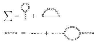
Figure 1: The self-consistent diagrammatic equations for the Green function and mass operator. Here ${\Sigma}$ is the mass operator. The double solid line denotes the total Green function $G.~{}$ The wavy line represents the interaction (2) and the double wavy line corresponds to the renormalized interaction.

The first diagrammatic equation in Fig.1 reads

$$\Sigma_{\alpha,\sigma}\left(\varepsilon,p\right) = \Sigma_{\alpha,\sigma}^{(1)}\left(\varepsilon,p\right)+\Sigma_{\alpha,\sigma}^{(2)}\left(\varepsilon,p\right),$$ (3)

$$\Sigma_{\alpha,\sigma}^{(1)}\left(\varepsilon,p\right) = \frac{T}{V}\sum_{\alpha^{\prime}\sigma^{\prime}\mathbf{k}\omega}U_{\alpha\alpha^{\prime}}\left(0\right)G_{\alpha^{\prime}\sigma^{\prime}}\left(\mathbf{k},\omega\right),$$ (4)

$$\Sigma_{\alpha,\sigma}^{\left(2\right)}\left(\varepsilon,p\right) = -\frac{T}{V}\sum_{\mathbf{k}\omega}\widetilde{U}_{\alpha\alpha}\left(\mathbf{k},\omega\right)G_{\alpha\sigma}\left(\mathbf{p}+\mathbf{k},\varepsilon+\omega\right).$$ (5)

Here $T$ is the temperature, and $V$ is the square of the layers.

The renormalized interaction $\widetilde{U}_{\alpha\alpha}\left(\mathbf{p},\omega\right)$ in Eq. (5) obeys the second diagrammatic equation in Fig.1 and reads

$$\widetilde{U}_{\alpha\alpha}\left(\mathbf{p},\omega\right)=U_{\alpha\alpha}\left(\mathbf{p}\right)+U_{\alpha\alpha}\left(\mathbf{p}\right)\Pi_{\alpha\sigma}\left(\mathbf{p},\varepsilon\right)\widetilde{U}_{\alpha\alpha}\left(\mathbf{p},\omega\right).$$ (6)

The polarization operator

$$\Pi\left(\mathbf{p},\varepsilon\right)=\Pi_{\alpha\sigma}\left(\mathbf{p},\varepsilon\right)=\frac{T}{V}\sum\limits_{\mathbf{k}\omega}G_{\alpha\sigma}\left(\mathbf{p}+\mathbf{k,}\varepsilon+\omega\right)G_{\alpha\sigma}\left(\mathbf{k},\omega\right)$$ (7)

does not depend on the kind of the particles.

Let us explain the rule of diagram selection. Each fermion loop contributes a factor $\nu$ to the diagrams. Among all the diagrams of the given order, only the diagrams are retained which contain the maximal number of the fermion loops. Thus, our approach is a $1/\nu$ expansion which results in keeping only the diagram of the RPA kind. The diagrams for which the bubbles are linked by more than one interaction line are small as compared with the RPA ones in the parameter $1/\nu.$For the same reason, the diagrams are small, which contain any vertex corrections.

The expression for the renormalized interaction follows from Eq. (6)

$$\widetilde{U}_{\alpha\alpha}\left(\mathbf{p},\omega\right)=\widetilde{U}\left(\mathbf{p},\omega\right)=\frac{U_{\alpha\alpha}\left(\mathbf{p}\right)}{1-\nu\cdot U_{\alpha\alpha}\left(\mathbf{p}\right)\Pi\left(\mathbf{p},\omega\right)}.$$ (8)

Let us note that, like the polarization operator $\Pi_{\alpha\sigma}\left(\mathbf{p},\omega\right)$, both the mass operator $\Sigma_{\alpha,\sigma}\left(\varepsilon,p\right)$ and the renormalized interaction $\widetilde{U}_{\alpha\alpha}\left(\mathbf{p},\omega\right)$ do not depend on the kind of the particle.

Our first goal is to calculate the chemical potential $\mu$ as a function of the density $n$ using the self-consistent system of Eqs. (3)-(8). Let us remind the exact relation

$$\mu-\Sigma\left(0,p_{F}\right)=p_{F}^{2}/2.$$ (9)

Then, the convergence method is used. If the interaction is neglected, the mass operator $\Sigma\left(0,p_{F}\right)\approx 0$ and, therefore,

$$\mu\approx\mu_{0}=p_{F}^{2}/2=2\pi n/\nu.$$ (10)

To find the next iteration for the chemical potential, let us calculate $\Sigma\left(0,p_{F}\right)$ taking $\mu=\mu_{0}$. In this case, one should replace $G$ by $G_{0}$ in the above system of equations. First, taking into account Eq. (2), we obtain

$$\Sigma_{\alpha\sigma}^{(1)}\left(\varepsilon,\mathbf{p}\right)=\frac{T}{V}\sum_{\alpha^{\prime}\sigma^{\prime}\mathbf{k}\omega}U_{\alpha\alpha^{\prime}}\left(0\right)G_{\alpha^{\prime}\sigma^{\prime}}^{0}\left(\mathbf{k},\omega\right)=2\pi ln.$$ (11)

Then, to find the next contribution to the mass operator $\Sigma_{\alpha\sigma}^{2}\left(\omega,\mathbf{p}\right),$ one should first estimate the renormalized interaction $\widetilde{U}_{\alpha\alpha}\left(\mathbf{k},\omega\right)$. For this purpose, let us consider the polarization operator in zero order in the interaction:

$$\Pi\left(\mathbf{p},\varepsilon\right)\approx\frac{1}{\left(2\pi\right)^{2}}\int d^{2}k\frac{n_{0}\left(\mathbf{k}\right)-n_{0}\left(\mathbf{k+p}\right)}{i\hbar\varepsilon+\mathbf{k}^{2}/2-\left(\mathbf{k+p}\right)^{2}/2},$$ (12)

where $n_{0}\left(\mathbf{k}\right)=\left[\exp\frac{\left(k^{2}/2-\mu_{0}\right)}{T}+1\right]^{-1}$ is the Fermi distribution function.

For small momenta and frequencies $p\lesssim p_{F},$ $\varepsilon\lesssim\varepsilon_{F},$ one finds $\Pi_{0}\left(\mathbf{p},\varepsilon\right)\simeq-1/2\pi.$ Substituting this value into Eq. (8) gives the estimate

$$\widetilde{U}\left(\mathbf{p},\varepsilon\right)=\frac{U_{\alpha\alpha}\left(\mathbf{p}\right)}{1+U_{\alpha\alpha}\left(\mathbf{p}\right)\nu\frac{1}{2\pi}}\simeq\frac{1}{\nu}\ll 1.$$ (13)

This estimation is valid if

$$n^{1/3}/\nu\ll 1,$$ (14)

what is supposed below.

Let us turn to the behavior of the renormalized interaction $\widetilde{U}\left(\mathbf{p},\varepsilon\right)$ for  large momenta  $\left|\mathbf{p}\right|\gg p_{F}.$ First, let us estimate the polarization operator (12) for such momenta. Consider, for example, the contribution $\Pi^{\prime}\left(\mathbf{p},\varepsilon\right)$ associated with the factor $n_{\alpha\sigma}\left(\mathbf{p}+\mathbf{q}\right).$ It is evident that momenta $\mathbf{k}$ alone contribute to the polarization operator for which $\left|\mathbf{p}+\mathbf{k}\right|\leq p_{F}.$ For this reason,  $\left|\mathbf{k}\right|\gg p_{F}.$ Therefore, $\left(\mathbf{p}+\mathbf{k}\right)^{2}\ll\mathbf{k}^{2}\approx\mathbf{p}^{2}$ and

$$\Pi^{\prime}\left(\mathbf{p},\varepsilon\right)\approx-\frac{1}{\left(2\pi\right)^{2}}\frac{n/\nu}{i\hbar\varepsilon+\mathbf{p}^{2}/2}.$$

Similarly, one can estimate the contribution $\Pi_{0}^{\prime\prime}\left(\mathbf{p},\varepsilon\right)$ connected with the term $n_{\mathbf{p}}$ in Eq. (12). As a result, we obtain

$$\Pi\left(\mathbf{p},\varepsilon\right)\approx-\frac{1}{\left(2\pi\right)^{2}\nu}\frac{n\mathbf{p}^{2}}{\varepsilon^{2}+\left(\mathbf{p}^{2}/2\right)^{2}},~{}p\gg p_{F}.$$ (15)

Taking into account (15), one can estimate the renormalized interaction (8)

$$\widetilde{U}\left(\mathbf{p},\omega\right)=\frac{\frac{2\pi}{p}}{1+\frac{2\pi}{p}\frac{np^{2}}{\omega^{2}+\left(p^{2}/2\right)^{2}}},~{}p\gg p_{F}.$$ (16)

Substituting (13) into (5) gives the estimate for the contribution to the self-energy $\Sigma_{\alpha\sigma}^{\left(2\right)}\left(\omega,\mathbf{p}\right)$ coming from $\left|\mathbf{k}\right|\leq p_{F}.$

$$\left|\Sigma_{\alpha,\sigma}^{\prime\left(2\right)}\left(\varepsilon,p\right)\right|\approx\frac{1}{\pi}\frac{n}{\nu^{2}}.$$ (17)

Let us turn to the contribution to $\Sigma_{\alpha\sigma}^{\left(2\right)}\left(\omega,\mathbf{p}\right)$ gained from $\left|\mathbf{k}\right|\gg p_{F}.$ It is convenient to represent it in the form

$$\Sigma_{\alpha,\sigma}^{\prime\prime\left(2\right)}\left(\varepsilon,p\right)=-\frac{T}{V}\sum_{\left|\mathbf{k}\right|\gg p_{F},~{}\omega}(U\left(\mathbf{k}\right)G_{\alpha\sigma}^{0}\left(\mathbf{p}+\mathbf{k},\varepsilon+\omega\right)-$$

$$-\frac{T}{V}\Delta U\left(\mathbf{k}\right)G_{\alpha\sigma}^{0}\left(\mathbf{p}+\mathbf{k},\varepsilon+\omega\right)).$$ (18)

Here $\Delta U\left(\mathbf{k}\right)=\widetilde{U}\left(\mathbf{k},\omega\right)-U\left(\mathbf{k}\right).$ The first sum on the R.H.S. in Eq. (18) can be estimated as

$$\frac{1}{\left(2\pi\right)^{2}}\int_{\left|\mathbf{k}\right|\gg p_{F}}\frac{d^{2}\mathbf{k}}{\left|\mathbf{k}\right|}n_{0}\left(\mathbf{k+p}\right)\leq\frac{1}{\pi^{3/2}}\left(\frac{n}{\nu}\right)^{1/2}$$ (19)

Let us turn to the second term on the R.H.S. in Eq. (18). Since we are interested in $\Sigma_{\alpha,\sigma}^{\prime\prime 2}\left(0,p_{F}\right),$ let us substitute $\left[G_{\alpha\sigma}^{0}\left(\mathbf{p}+\mathbf{k},\varepsilon+\omega\right)+G_{\alpha\sigma}^{0}\left(\mathbf{p}-\mathbf{k},\varepsilon-\omega\right)\right]\approx$ $-\frac{k^{2}}{\omega^{2}+\left(k^{2}/2\right)^{2}}\left(k\gg p_{F}\right)$ into this term. Then, one obtains the estimate for the second sum in Eq. (18)

$$-\frac{1}{\left(2\pi\right)^{3}}\int d\omega\int_{k\gg p_{F}}kdk\frac{\left(\frac{2\pi}{k}\right)^{2}n\left(\frac{k^{2}}{\omega^{2}+\left(k^{2}/2\right)^{2}}\right)^{2}}{1+\frac{2\pi}{k}\frac{nk^{2}}{\omega^{2}+\left(k^{2}/2\right)^{2}}}\approx-Cn^{1/3}.$$ (20)

This estimate results from the following hint. Let us introduce new variables $\omega/n^{2/3}$ and $k=k/n^{1/3}$. The integrand is maximal in the vicinity of the region $\omega/n^{2/3}$ $\sim k/n^{1/3}\sim 1.$ Due to Eq. (14), one can put the lower limit equal to zero in integral (20). Then the integral depends on the concentration as $n^{1/3}.$ The proportionality constant is calculated numerically, $C\approx 0.615$.

III Equation of state

Taking into account condition (14), one can neglect the contribution of expressions (10) (17), (19) into the chemical potential as compared with (20). Thus, expressions (11) and (20) alone contribute to the chemical potential. Therefore,

$$\mu\approx 2\pi ln-Cn^{1/3}.$$ (21)

The chemical potential $\mu,$ given by Eq. (21), is a result of the first iteration. Let us now substitute expression (21) for the chemical potential into Eqs. (3) - (5) instead of $\mu_{0}$ and repeat all the calculations starting from Eq. (11). It is easy to find that, whether $\mu_{0}$ or $\mu$ is taken as a starting point, the correlation contribution to the self-energy is of the same order of the magnitude given by (20). For this reason, the expression for the chemical potential (21) is the stable solution of the self-consistent system of equations, the constant $C$ being of the order of unity. This chemical potential corresponds to the energy per unit volume

$$\varepsilon=\pi ln^{2}-\frac{3}{4}Cn^{4/3}.$$ (22)

Then, at zero temperature the pressure is

$$P=\mu n-\varepsilon=\pi ln^{2}-\frac{C}{4}n^{4/3}.$$ (23)

At small density $n<$ $\left(C/6\pi l\right)^{3/2},$ the compressibility $\partial P/\partial V>0,$ and the system is unstable. For higher density, in the interval $\left(C/6\pi l\right)^{3/2}<n<\left(C/4\pi l\right)^{3/2}$, one has $\partial P/\partial V<0.$ The system is stable and has a negative pressure. The liquid state is reached at the upper limit of this interval

$$n_{eq}=\left(C/4\pi l\right)^{3/2}.$$ (24)

where the pressure $P=0.$

Thus, for the electron-hole liquid in the equilibrium, the bound energy per one particle is

$$\varepsilon_{eq}=-\varepsilon\left(n_{eq}\right)/n_{eq}=-\frac{C^{3/2}}{4\pi^{1/2}}\frac{1}{l^{1/2}}.$$ (25)

At the same time, for the isolated exciton the bound energy $\varepsilon_{ex}^{0}~{}$is known to behave as $\varepsilon_{ex}^{0}\sim-1/l.$ Since the excitons in the CQW experience repulsion,. the bound energy per particle is $\varepsilon_{ex}>-1/l.$ Comparing this energy with $\varepsilon_{eq}$ (see expression (25)) one concludes that the electron-hole state possesses a smaller energy as compared to the exciton state for $l\gg 1$. In addition, note that the exciton in-plane radius $R_{ex}\sim l^{3/4}$ and, thus, for the equilibrium carrier concentration obtained, one has $n_{eq}R_{ex}^{2}\sim 1.$ Under such conditions, the exciton concept seems us to have no sense.

IV Discussion and Conclusion

The results above are obtained for the case $l\gg 1,$ i.e., $l\gg a_{B}.$ In this case, the ground-state of the system is the electron-hole liquid which possesses the equilibrium density (24). This is a stable state which has the energy smaller than that of the exciton state.

Consider, however, the case $l\ll 1.$ It follows from Eqs. (10), (11), (20) that the kinetic energy $\varepsilon_{kin}$, the direct Coulomb interaction $\varepsilon_{eh}$ and the intra-layer correlation energy $\varepsilon_{corr}$ can be estimated as

$$\varepsilon_{kin}\sim\frac{n}{\nu},\varepsilon_{e-h}\sim nl,\varepsilon_{corr}\sim-n^{1/3},$$

respectively. The equilibrium is reached at the concentration

$$n_{eq}\sim\left(\frac{\nu}{1+\nu l}\right)^{3/2},$$ (26)

for which the total energy $\varepsilon_{eq}$ is minimal and

$$\varepsilon_{eq}\sim-\left(\frac{\nu}{1+\nu l}\right)^{1/2}\approx\left\{\begin{array}[]{c}-\frac{1}{l},\text{if~{}}\nu l\gg 1\\ -\nu^{1/2},\text{if~{}}\nu l\ll 1\end{array}\right..$$ (27)

For the case $l\ll 1$ considered in this place, the exciton bound energy $\varepsilon_{ex}\sim-1$ in the units taken in the paper. (In fact, this energy is even larger due to repulsion between the excitons). Throughout the paper it is assumed that $\nu\gg 1.$Thus, $\varepsilon_{eq}\ll\varepsilon_{ex},$ as well as above in the case $l\gg 1$. Also, for the concentration (26), the average distance between the carriers is of the order of $~{}n_{eq}^{-1/2}\sim$ $\left(\frac{1+\nu l}{\nu}\right)^{3/4}\ll 1.$ At the same time, for $l\ll 1$ the exciton in-plane radius $R_{ex}\sim a_{B}=1.$ Thus, the exciton in-plane radius $R_{ex}$ exceeds the average distance between the carriers, what has no sense. Thus, both in the case $l\gg 1$ and in the case $l\ll 1$ the ground state of the system of spatially separated electrons and holes in the CQW is the electron-hole liquid.

As the intermediate case $l\sim 1$ is concerned, both $\varepsilon_{eq}$ $\sim-1$ and $\varepsilon_{ex}\sim-1.$ However, in this case $n_{eq}^{-1/2}\sim R_{ex}\sim a_{B}\sim 1$ and, thus, the exciton concept seems has no sense as well.

Let us return to the case $l\gg 1.$An interesting feature of the results obtained is that both the bound energy (24) and the equilibrium concentration (25) of the electron-hole liquid in the CQW do not depend on the parameter $\nu.$ This is in spite of the fact that formally this parameter was supposed to be large. This circumstance allows us to expect that the liquid equilibrium electron-hole state in the CQW may arise even for $\nu\sim 1.$ However, for $\nu\gg 1,$ the kinetic energy, which is of the order of $\varepsilon_{F}\sim\frac{1}{\nu},$ plays an insignificant role in the formation of the equilibrium state. The equilibrium within the electron-hole system is reached due to balance between the positive direct Coulomb interaction (11) and the negative in-layer correlation energy (20).

Let us pay attention to the interesting feature of the origin for the correlation energy associated with the RPA diagram. The correlation energy contribution results from the momentum transfer $p\sim n^{1/3}\gg p_{F}.$ This conclusion strongly differs from that of Gell-Mann and Brueckner who considered the many-body correlations for a $3D$ electron gas. Within their approach, the correlation energy originates from the momentum transfer $p\ll p_{F}.$ Let us also point out additional arguments which approve the RPA approximation. While the Gell-Mann and Brueckner approach is justified for $n\gg 1,$ our approach holds for an arbitrary concentration $n$ provided that $\nu$ is large.

Let us investigate how the results obtained can be associated with the experiments. Below, we follow the scenario proposed by Keldysh for the electron-hole liquid formation in semiconductorskeldysh . Consider a non-equilibrium inhomogeneous electron-hole system in the CQW, composed of two coexisting phase: a rare exciton gas phase and a dense electron-hole liquid drops. Let $R$ be the characteristic radius of the drop and $\tau$ be the carrier (electron or hole) lifetime within this drop. Then, the loss of the carriers per unit time for the drop is $-\pi R^{2}n_{eq}/\tau.$ On the other hand, there exists an exciton flow $j$ in the gas phase, induced by an external source. This flow gains the number of carriers in the drop per unit time $+2\pi Rj.$ In the dynamic equilibrium, the loss and the gain balance each other, resulting in the dependence

$$R\approx\frac{2j\tau}{n_{eq}}.$$

The concept of the electron-hole drop in the CQW fails if $R<a_{B}=1.$Therefore, there exists a threshold value for the flow

$$j>j_{c}=\frac{n_{eq}a_{B}}{2\tau},$$ (28)

which provides the formation of the drop. Thus, if the flow $j$ is weak, the drop has no time to form.

Such a scenario may account for the appearance of luminescent rings in the CQW in the series of experiments Nature-2002-Butov ; Nature-2002-Snoke ; Butov2003 ; Snoke2003 ; Butov2004 ; Larionov2002 ; Dremin2004 ; Timofeev2005 . These rings, sometimes, are associated with the exciton Bose condensate. However, in our opinion, they should be connected with the electron-hole liquid drop described above. First of all for these experiments, the criterion of the exciton existence $R_{ex}^{2}n\ll 1$ seems to be violated. However, suppose that the core of the ring under the experiments is illuminated by the external optical pump resulting in the creation of the exciton gas flow $j$ within the core. Then, the ring corresponds to the electron-hole liquid phase described above. It follows from Eq. (28) that the electron-hole liquid ring can dwell in the stationary state if the flow $j$ exceeds a certain critical value. In the experiments, the luminescent ring appears if the optical pumping exceeds a certain power. Thus, the results obtained may be the basis for the explanation of these experiments.

Let us mention that the correlation energy calculated above does not involve the effect of the exciton-like electron-hole correlation associated with the ladder diagrams in the electron-hole scattering channel. The involvement of this effect would result in the appearance of the nonvanishing anomalous exciton-like averages responsible for the creation of the dielectric gap on the Fermi surfaceKO . However, the contribution of these diagrams into correlation energy is small in the parameters $1/\nu.$This makes insignificant their influence on the thermodynamics of the system, the main subject of the paper.

We are grateful to Yuri Lozovik for valuable discussions.

References

- (1) Yu. E. Lozovik and V.I. Yudson, Zh. Exp.Theor. Fiz. 71, 738 (1976) [Sov. Phys. JETP 44, 389 (1976)].
- (2) K. Das Gupta, A.F. Croxall, J. Waldie, C.A. Nicoll, H.E. Beere, I. Farrer, D.A. Ritchie, and M. Pepper, Adv. Cond. Matt. Phys. Volume 2011, Article ID 727958.
- (3) Yu. Lozovik and O.L. Berman, JETP Lett. 64, 573 (1996)];JETP 84, 1027 (1997).
- (4) Yogesh N. Joglekar, Alexander V. Balatsky, and S. Das Sarma, 74, 233302 (2006)
- (5) E.A. Andrushin, V.S. Babichenko, L.V. Keldysh, et all. JETPh Lett, 24, 210 (1976).
- (6) L.V. Keldysh, Electron-Hole liquid in Semiconductors, in Morden Problems of Condense Matter Science, v. 6, C.D. Jeffries and L.V. Keldysh (North Holland, Amsterdam, 1987)
- (7) L. V. Keldysh, ”Excitones in Semiconductors”, (Nauka, Moscow, 1971).
- (8) T. M. Rice, “The electron-hole liquid in semiconductors”, Solid State Physics V 32, ed.: H. Ehrenreich, F. Zeitz, D. Turnbull, Academic Press, INC. 1077.
- (9) L.V. Butov, A.C. Gossard, and D.S. Chemla, Nature (London) 418, 751 (2002).
- (10) D. Snoke, S. Denev, Y. Liu, L. Pheiffer, and D.S. Chemla, Nature (London) 418, 754 (2002).
- (11) L.V. Butov, Solid State Commun. 127, 89 (2003).
- (12) D. Snoke, Y. Liu, S. Denev, L. Pheiffer, and K. West. Solid State Commun. 127, 187 (2003).
- (13) L.V. Butov, L.S. Levitov, A.V. Mintsev, B. D. Simons, A.C. Gossard, and D.S. Chemla, Phys. Rev. Lett. 92, 117404 (2004)
- (14) A.V. Larionov, V.B. Timofeev, P.A. Ni, S.V. Dubonos, I. Hvam, and K. Soerensen, Pis’ma Zh. Ekp. Theor. Fiz. 75, 233 (2002) [JETP Lett. 75, 570 (2002)].
- (15) A.A. Dremin, A.V. Larionov, and V. B. Timofeev, Fiz. Tverd. Tela (St. Peterburg) 46, 168 (2004) [Solid. State. Phys. 46, 170 (2004)].
- (16) V.B. Timofeev, Usp. Phys. Nauk 175, 315, (2005) [Phys. Usp. 48, 295 (2005)].
- (17) L.S. Levitov, B.D. Simons, and L.V. Butov, Phys. Rev. Lett, 94, 176404 (2005).
- (18) L.V. Keldysh, and Yu.V. Kopaev, Sov. Phys. Solid State 6, 2219 (1965).