Unified Bertotti-Robinson and Melvin Spacetimes

Abstract

We present a solution for the Einstein-Maxwell (EM) equations which unifies both the magnetic Bertotti-Robinson (BR) and Melvin (ML) solutions as a single metric in the axially symmetric coordinates $\left\{t,\rho,z,\varphi\right\}$. Depending on the strength of magnetic field the spacetime manifold, unlike the cases of separate BR and ML spacetime, develops singularity on the symmetry axis ($\rho=0$). Our analysis shows, beside other things that there are regions inaccessible to all null geodesics.

I Introduction

The Bertotti-Robinson (BR) 1 and Melvin (ML) 2 solutions of Einstein-Maxwell (EM) theory are well-known for a long time which had significant impacts on different aspects of general relativity. For decades they remained in fashion and found applications in connection with stellar objects, cosmology, string theory etc. A recent study discusses the similarities / differences between these spacetimes 3 . It is shown, among other things in 3 for instance, that the only geodesically complete static EM spacetimes are the BR and ML solutions. Since they share  more common properties than contrasts, the natural question arises whether it is possible to describe both solutions in a common metric. This is precisely what we show in the axially symmetric (i.e. $t,$ $\rho,$ $z,$ $\varphi$ coordinates) geometry in this paper. It should be added that large classes of EM solutions found long ago by Kundt 4 and Plebanski and Demiahski (PD) 5 ; 6 both admitted separate BR and ML limits in different coordinates through specific limits. We work out our solution entirely in the axially symmetric $\left\{t,\rho,z,\varphi\right\}$ coordinates and express our metric in those coordinates. Our solution admits the BR limit but not the separate ML limit. In other words BR universe forms the background of our spacetime on which ML is added. In obtaining the solution we choose the magnetic phase of BR solution so that the total magnetic potential $\psi\left(\rho,z\right)$ is expressed as a superposition, $\psi\left(\rho,z\right)=$ $\psi_{BR}\left(\rho,z\right)+$ $\psi_{ML}\left(\rho,z\right).$ The EM solution constructed from $\psi\left(\rho,z\right)$ is what we dub as the ”unified BR and ML spacetime”. The solution involves two parameters, $\lambda_{0}$ (for BR charge) and $B_{0}$ (for ML charge). The ranges of parameters are $0<\left|\lambda_{0}\right|<\infty$ and $-\infty<B_{0}<\infty,$ so that our solution doesn’t admit the ML limit.

BR spacetime is conformally flat whereas ML is cylindrically symmetric which becomes flat near the axis $\rho\rightarrow 0.$ For a finite $\rho$ and $\left|z\right|\rightarrow\infty$ ML is not flat. Both are singularity free; a feature that makes them attractive in cosmology and string theory. We remark also that the BR solution can be obtained by a coordinate transformation 7 from a spacetime of colliding electromagnetic waves known as Bell-Szekeres solution 8 . Using the Ernst formalism we showed long ago that within this formalism Bell-Szekeres and Khan-Penrose 9 solutions can be combined through a suitable seed function 10 . Also Schwarzschild and BR spacetimes were interpolated by the electromagnetic parameter in the oblate spheroidal coordinates 11 . Within similar context superposition of spinning spheroids 12 from harmonic seed functions in the Zipoy-Voorhees metric 13 were obtained. It is remarkable that interpolation of BR and ML solutions takes place in the static axial coordinates $\left(\rho,z\right)$ instead of oblate/ prolate coordinates. The latter coordinate systems are known to admit separability in the Laplace equation and had much impact in the development of solution generation techniques. One of the important conclusions to be drawn in this study is that two electromagnetic fields, which separately yield regular spacetimes, namely the BR and ML, may yield a singular spacetime upon their combination. Physical interpretation suggests that the mutual magnetic fields focus each other strong enough to result in a singularity. The singularity at $\rho=z=0$ (for $\frac{B_{0}}{\lambda_{0}}<0$ and $\frac{B_{0}}{\lambda_{0}}>1$) doesn’t exhibit directional properties 14 , that is, the Kretschmann scalar diverges irrespective of the way of approach and ($\rho=0,z>0$) is the only singularity in our solution for arbitrary parameters. An exact solution of null geodesics reveals that we have a null-geodesically incomplete manifold. Beside null geodesics we study the radial motion for massless / massive particles and also the circular motion in the $z=0$ plane. From the analysis of the potential the circular motion admits stable orbits.

Organization of the paper is as follows. In Sec. II we introduce magnetic fields in axial symmetry, solve the equations and derive the metric of Unified BR and ML spacetimes. Geodesic equation and its solutions are investigated in Sec. III. The paper ends with Conclusion in Sec. IV.

II Magnetic fields in static axial symmetry

To review the basics of an axially symmetric spacetime we start with the line element

$$ds^{2}=-e^{2U}dt^{2}+e^{-2U}\left[e^{2K}\left(d\rho^{2}+dz^{2}\right)+\lambda^{2}d\varphi^{2}\right]$$ (1)

in which $U,$ $K$ and $\lambda$ are functions of $\rho$ and $z$ alone. The EM field equations can be derived from a variational principle of the action

$$I=\int Ld\rho dz$$ (2)

where

$$L=K_{\rho}\lambda_{\rho}+K_{z}\lambda_{z}-\lambda\left[U_{\rho}^{2}+U_{z}^{2}-e^{-2U}\left(\psi_{\rho}^{2}+\psi_{z}^{2}\right)\right].$$ (3)

Here $f_{\rho}$ $/$ $f_{z}$ denotes partial derivative of a function $f\left(\rho,z\right)$ with respect to $\rho$ $/$ $z$ and $\psi$ is a magnetic potential. Upon variation the metric function $\lambda$ is fixed as $\lambda=\rho$, while the two basic equations take the forms

$$\left(\rho U_{\rho}\right)_{\rho}+\rho U_{zz}-\rho e^{-2U}\left(\psi_{\rho}^{2}+\psi_{z}^{2}\right)=0$$ (4)

$$\left(\rho e^{-2U}\psi_{\rho}\right)_{\rho}+\rho\left(e^{-2U}\psi_{z}\right)_{z}=0.$$ (5)

The $K$ function is determined more appropriately by the set

$$K_{\rho}=\rho\left(U_{\rho}^{2}-U_{z}^{2}\right)+\rho e^{-2U}\left(\psi_{z}^{2}-\psi_{\rho}^{2}\right)$$ (6)

$$K_{z}=2\rho U_{\rho}U_{z}-2\rho e^{-2U}\psi_{\rho}\psi_{z}$$ (7)

whose integrability condition is satisfied by virtue of the field equations. The magnetic vector potential is chosen simply by

$$A_{\mu}=\delta_{\mu}^{\varphi}\Phi$$ (8)

for a function $\Phi\left(\rho,z\right)$ which is related to $\psi$ above through

$$\Phi_{\rho}=\rho e^{-2U}\psi_{z}$$ (9)

$$\Phi_{z}=-\rho e^{-2U}\psi_{\rho}.$$ (10)

The dual of the field tensor ${}^{\star}F_{ti}=\psi_{i}$ implies the absence of any electric components which is our choice here. In 3 BR and ML solutions are summarized in details so that we can only record them in what follows:

II.1 BR and ML solutions

II.1.1 The BR solution

$$U=U_{BR}=\ln\lambda_{0}+\frac{1}{2}\ln\left(\rho^{2}+z^{2}\right)$$ (11)

$$\psi=\psi_{BR}=\lambda_{0}\sqrt{\rho^{2}+z^{2}}$$ (12)

$$K = K_{BR}=\text{const.}$$

$$\left(\lambda_{0}=\text{constant.}\right)$$

Note that the more familiar $AdS_{2}\times S^{2}$ version of BR spacetime is given upon the transformation

$$\rho=\frac{\sin\theta}{r},$$ (14)

$$z=\frac{\cos\theta}{r},$$ (15)

by

$$ds^{2}=\frac{1}{r^{2}}\left(-dt^{2}+dr^{2}\right)+d\theta^{2}+\sin^{2}\theta d\varphi^{2}.$$ (16)

II.1.2 The ML solution

$$U=U_{ML}=\ln\left(1+\frac{B_{0}^{2}}{4}\rho^{2}\right)$$ (17)

$$\psi=\psi_{ML}=B_{0}z$$ (18)

$$K = K_{ML}=2\ln\left(1+\frac{B_{0}^{2}}{4}\rho^{2}\right)$$

$$\left(B_{0}=\text{constant.}\right)$$

II.2 A combined BR and ML solution

We proceed now to combine the foregoing solutions. For this purpose we take the magnetic potential as the superposition of the two foregoing, namely

$$\psi=\psi_{BR}+\psi_{ML}=\lambda_{0}\sqrt{\rho^{2}+z^{2}}+B_{0}z$$ (20)

where $B_{0}$ and $\lambda_{0}$ are the constants of ML and BR solutions which are restricted by $0<\left|\lambda_{0}\right|<\infty$ and $-\infty<B_{0}<\infty$. To get an idea about this superposition we resort to the axial gauge $A_{\mu}=\left(0,0,0,A_{\varphi}\right)$ in flat space

$$ds^{2}=-dt^{2}+d\rho^{2}+dz^{2}+\rho^{2}d\varphi^{2}.$$ (21)

Let $A_{\varphi}^{\left(1\right)}=\lambda_{0}\sqrt{\rho^{2}+z^{2}}$ and $A_{\varphi}^{\left(2\right)}=B_{0}z$ be two magnetic potentials where both solve the Maxwell equations $\partial_{\mu}F^{\left(i\right)\mu\nu}=0,$ ($i=1,2$) with $F_{\mu\nu}^{\left(i\right)}=\partial_{\mu}A_{\nu}^{\left(i\right)}-\partial_{\nu}A_{\mu}^{\left(i\right)}.$ It can be checked easily that their superposition $A_{\mu}=\left(0,0,0,A_{\varphi}^{\left(1\right)}+A_{\varphi}^{\left(2\right)}\right)$ solves the superposed Maxwell equation $\partial_{\mu}\left[\rho\left(F^{1\mu\nu}+F^{2\mu\nu}\right)\right]=0.$ Upon this observation we seek an analogous behavior in the curved spacetime and we find out that indeed it works with some difference. Integration of the field equations from Eq. (4) to Eq. (7) yields the following results

$$e^{U}=F$$ (22)

$$e^{K}=\frac{F^{2}}{\rho^{2}+z^{2}}\left(\frac{\rho^{1+\frac{B_{0}}{2\lambda_{0}}}}{z+\sqrt{\rho^{2}+z^{2}}}\right)^{\frac{2B_{0}}{\lambda_{0}}}$$ (23)

where the function $F$ is given by

$$F=\lambda_{0}\left[\sqrt{\rho^{2}+z^{2}}\cosh\left(\frac{B_{0}}{\lambda_{0}}\ln\rho\right)-z\sinh\left(\frac{B_{0}}{\lambda_{0}}\ln\rho\right)\right].$$ (24)

It is observed easily that setting $B_{0}=0$ recovers the BR solution with a charge $\lambda_{0}$. However, the limit $\lambda_{0}=0$ does not exist, which means that although in flat spacetime our electromagnetic field is a superposition of BR and ML potentials, in curved spacetime the solution gives only the BR limit correctly. This is in contrast with the $7-$parametric PD class of EM solutions 5 ; 6 which admits electromagnetic fields even in the flat space limit. In our case existence of the BR is essential while ML limit can’t be interpolated. Let us add also that the metric functions of PD are expressed in its most generality in quartic polynomial forms whereas our solution involves decimal powers as well. These distinctive properties suggest that our solution is not included in the general class of PD. The two are expressed in different coordinates / symmetries so that transition between the two for arbitrary cases can’t be expressed in closed forms. More specifically, the type-D metric of PD class that yields separately the ML and BR limits are as follows: i)

$$ds_{ML}^{2}=p^{2}\left(-Q\left(p\right)d\bar{t}^{2}+\frac{dq^{2}}{Q\left(q\right)}\right)+\\ \frac{P\left(p\right)}{p^{2}}d\bar{\sigma}^{2}+\frac{p^{2}}{P\left(p\right)}dp^{2}.$$ (25)

Letting $Q\left(q\right)=1,$ $P\left(p\right)=\frac{4}{B_{0}^{2}}\left(p-1\right),$ ($B_{0}=$constant), $p=1+\frac{B_{0}^{2}}{4}\rho^{2},$ $q=\frac{B_{0}^{2}}{2}z,$ $\bar{\sigma}=\varphi,$ and an overall scaling gives the ML metric. ii)

$$ds_{BR}^{2}=b^{2}\left(-Q\left(p\right)dt^{2}+\frac{dq^{2}}{Q\left(q\right)}\right)+\\ \gamma^{2}\left(\frac{P\left(p\right)}{p^{2}}d\sigma^{2}+\frac{p^{2}}{P\left(p\right)}dp^{2}\right).$$ (26)

Letting $b=\gamma=1,$ $Q\left(q\right)=q^{2}=\rho^{2}+z^{2},$ $P\left(p\right)=1-p^{2}=\frac{\rho^{2}}{\rho^{2}+z^{2}},$ $\sigma=\varphi,$ gives the BR metric in axial symmetry with a unit charge. It remains to be seen, however that (25) and (26) follow from the PD class of solutions in the same coordinate patch i.e. without further transformations in the ($p,q$) coordinates.

Furthermore it is worthful to look at the form of invariants of the spacetime. The complete form of the Kretschmann scalar is complicated enough that we only give it in a series form around $z=0$ i.e.,

$$\mathcal{K}=\frac{\rho^{-4\beta^{2}+4\beta}\left[A_{1}+A_{2}\rho^{2\beta}+A_{3}\rho^{4\beta}+A_{4}\rho^{6\beta}+A_{5}\rho^{8\beta}\right]}{\lambda_{0}^{4}\left(1+\rho^{2\beta}\right)^{8}}+\\ \frac{\rho^{-4\beta^{2}+4\beta-1}\left[B_{1}+B_{2}\rho^{2\beta}+B_{3}\rho^{4\beta}+B_{4}\rho^{6\beta}+B_{5}\rho^{8\beta}+B_{6}\rho^{10\beta}+B_{7}\rho^{12\beta}+B_{8}\rho^{14\beta}\right]}{\lambda_{0}^{4}\left(1+\rho^{2\beta}\right)^{11}}z+\\ \frac{\rho^{-4\beta^{2}+4\beta-2}\left[C_{1}+C_{2}\rho^{2\beta}+C_{3}\rho^{4\beta}+C_{4}\rho^{6\beta}+C_{5}\rho^{8\beta}+C_{6}\rho^{10\beta}+C_{7}\rho^{12\beta}+C_{8}\rho^{14\beta}+C_{9}\rho^{16\beta}+C_{10}\rho^{18\beta}+C_{11}\rho^{20\beta}\right]}{\lambda_{0}^{4}\left(1+\rho^{2\beta}\right)^{14}}z^{2}+\\ \mathcal{O}\left(z^{3}\right),$$ (27)

in which $\beta=\frac{B_{0}}{\lambda_{0}}\neq 0$ and $A_{i}$, $B_{i}$ and $C_{i}$ are all some polynomial functions of $\beta$ only. Having up to second order explicitly is enough to conclude that the solution is singular at $\rho=0$ and $z\neq 0$ for all values of $\beta.$ This is due to the term $C_{1}\frac{\rho^{-4\beta^{2}+4\beta-2}}{\lambda_{0}^{4}\left(1+\rho^{2\beta}\right)^{14}}z^{2}$ and $B_{1}\frac{\rho^{-4\beta^{2}+4\beta-1}}{\lambda_{0}^{4}\left(1+\rho^{2\beta}\right)^{11}}z$ which for $z\neq 0$ diverge for all $\beta.$ The coefficients $C_{1}$ and $B_{1}$ are given explicitly by

$$B_{1}=2048\left(\beta-\frac{1}{2}\right)\times\\ \left(\beta^{6}-3\beta^{5}+\frac{31}{4}\beta^{4}-\frac{21}{2}\beta^{3}+16\beta^{2}-\frac{45}{4}\beta+\frac{9}{2}\right)$$ (28)

and

$$C_{1}=256\left(-692\beta^{5}+380\beta^{6}+855\beta^{2}+63\right.-\\ \left.128\beta^{7}+1100\beta^{4}-351\beta-1196\beta^{3}+32\beta^{8}\right)$$ (29)

which can not be both zero. At $z=0$

$$\mathcal{K}=\\ \frac{\rho^{-4\beta^{2}+4\beta}}{\lambda_{0}^{4}\left(1+\rho^{2\beta}\right)^{8}}\left[A_{1}+A_{2}\rho^{2\beta}+A_{3}\rho^{4\beta}+A_{4}\rho^{6\beta}+A_{5}\rho^{8\beta}\right]$$ (30)

which for regularity at $\rho=0$ we must have

$$-4\beta^{2}+4\beta\geq 0.$$ (31)

We add that

$$A_{1}=\\ 768-2304\beta+3328\beta^{2}-2304\beta^{3}+1792\beta^{5}+256\beta^{6}$$ (32)

which has no real roots. The condition (31) implies that for $0\leq\beta\leq 1$ the origin is a regular point. Having clarified the role of the BR parameter $\lambda_{0}$, i.e. that $\lambda_{0}\neq 0$, so that in the rest of our analysis we may set $\lambda_{0}=1$ without loss of generality. In brief for $z=0$ and $\rho=0$ the solution is regular if $0\leq\frac{B_{0}}{\lambda_{0}}\leq 1$ and singular for other values of $\frac{B_{0}}{\lambda_{0}}$. Once more we recall that $\beta=\frac{B_{0}}{\lambda_{0}}=0$ corresponds to the BR limit whose Kretschmann scalar is $\frac{8}{\lambda_{0}^{4}}$ and the solution is regular everywhere. The Maxwell $2-$form of our solution is expressed by

$$F=\left(\Phi_{\rho}d\rho+\Phi_{z}dz\right)\wedge d\varphi$$ (33)

where $\Phi_{\rho}$ and $\Phi_{z}$ are defined by (9) and (10). As a result we obtain for the Maxwell invariants

$$I_{1}=\frac{1}{2}F_{\mu\nu}F^{\mu\nu}=\lambda_{0}^{2}e^{-2K}\left(1+\frac{B_{0}^{2}}{\lambda_{0}^{2}}+\frac{2B_{0}z}{\lambda_{0}\sqrt{\rho^{2}+z^{2}}}\right),$$ (34)

$$I_{2}=\frac{1}{2}F_{\mu\nu}{}^{\star}F^{\mu\nu}=0$$ (35)

in which $K$ was found in (23).

Nevertheless the following transformations

$$\zeta = \rho+iz$$ (36)

$$du = dt-\rho e^{-2U}d\varphi$$

$$dv = -2e^{2U}dt$$

casts (1) into the Kundt form 4

$$ds^{2}=du\left(dv+Hdu\right)+P^{-2}d\zeta d\bar{\zeta}$$ (37)

in which $H=e^{2U}$ and $P=e^{\left(K-U\right)}.$

III Geodesic Motion in cylindrical coordinates

The geodesic equations for the metric given in (1) are (without loss of generality we choose $\lambda_{0}=1$)

$$\frac{d}{ds}\left(\frac{\partial L}{\partial\dot{x}^{\mu}}\right)-\frac{\partial L}{\partial x^{\mu}}=0$$ (38)

in which

$$2L=-e^{2U}\dot{t}^{2}+e^{-2U}\left[e^{2K}\left(\dot{\rho}^{2}+\dot{z}^{2}\right)+\rho^{2}\dot{\varphi}^{2}\right]$$ (39)

and a dot means $\frac{d}{ds}.$ From the $t$ and $\varphi$ equations one finds

$$\dot{t}=Ee^{-2U},\text{ \ }\dot{\varphi}=\frac{\ell^{2}}{\rho^{2}}\text{\ }e^{2U}.$$ (40)

Using $L=\varepsilon=-1,+1,0$ for timelike, spacelike and null geodesics the other two equations are

$$\frac{d}{ds}\left(e^{-2U}e^{2K}\dot{\rho}\right)=-U_{\rho}E^{2}e^{-2U}+\left(K_{\rho}-U_{\rho}\right)\times\\ \left[\varepsilon+E^{2}e^{-2U}-\frac{\ell^{4}}{\rho^{2}}\text{\ }e^{2U}\right]-\frac{\ell^{4}}{\rho^{2}}U_{\rho}\text{\ }e^{2U}+\frac{\ell^{4}}{\rho^{3}}\text{\ }e^{2U}$$ (41)

and

$$\frac{d}{ds}\left(e^{-2U}e^{2K}\dot{z}\right)=-U_{z}E^{2}e^{-2U}+\left(-U_{z}+K_{z}\right)\times\\ \left[\varepsilon+E^{2}e^{-2U}-\frac{\ell^{4}}{\rho^{2}}\text{\ }e^{2U}\right]-\frac{\ell^{4}}{\rho^{2}}U_{z}\text{\ }e^{2U}.$$ (42)

We parametrize now $\rho$ with $z$ so that $\rho^{\prime}=\frac{d\rho}{dz}$and express geodesics in a single equation

$$\left(E^{2}e^{-2U}+\Delta+\frac{\ell^{4}}{\rho^{2}}\text{\ }e^{2U}\right)\left(U_{\rho}-\rho^{\prime}U_{z}\right)-\\ \Delta\left(K_{\rho}-K_{z}\rho^{\prime}\right)-+\frac{\ell^{4}}{\rho^{3}}\text{\ }e^{2U}+\frac{\Delta}{1+\rho^{\prime 2}}\rho^{\prime\prime}=0,$$ (43)

where $\Delta=\varepsilon+E^{2}e^{-2U}-\frac{\ell^{4}}{\rho^{2}}$ $e^{2U}.$ Let’s consider the null $\left(\varepsilon=0\right)$ geodesics in a plane of $\varphi=\varphi_{0}$ which implies $\ell=0$ and therefore (43) becomes (with $E^{2}=1$)

$$\left(2U_{\rho}-K_{\rho}\right)-\rho^{\prime}\left(2U_{z}-K_{z}\right)+\frac{\rho^{\prime\prime}}{1+\rho^{\prime 2}}=0.$$ (44)

The explicit form of latter equation reads as

$$\frac{d^{2}\rho}{dz^{2}}=2\left(1+\left(\frac{d\rho}{dz}\right)^{2}\right)\times\\ \left[\frac{z}{\rho^{2}+z^{2}}\left(\frac{d\rho}{dz}-\frac{\rho}{z}\right)+\frac{B_{0}}{\sqrt{\rho^{2}+z^{2}}}\left(\frac{d\rho}{dz}+\frac{z}{\rho}\right)+\frac{B_{0}^{2}}{2\rho}\right]$$ (45)

which is still complicated enough for an exact solution. Luckily we obtain an exact solution valid for $\left|B_{0}\right|>2$ given by

$$\rho=\left\{\begin{array}[]{ccc}\left(\left(\frac{B_{0}}{2}\right)^{2}-1\right)^{1/2}z,&B_{0}<-2,&z>0\\ -\left(\left(\frac{B_{0}}{2}\right)^{2}-1\right)^{1/2}z,&B_{0}>2,&z<0\end{array}\right..$$ (46)

As we stated above $\left|B_{0}\right|>2$ yields singularity at $\rho=z=0$, and our particular solution is valid only for this case. For each given $\left|B_{0}\right|>2$ we have a wedge region of $\left(\rho,z\right)$ which doesn’t cover all the $\left(\rho,z\right)$ plane. This is the indication that our particular solution doesn’t yield a null-geodesically complete spacetime. The BR and ML spacetimes are known both to be geodesically complete whereas our particular example provides a case of their combination which is at least null–geodesically incomplete. This can be observed by resorting to the solution (46) to obtain (let us choose $B_{0}=-4,$ for simplicity)

$$\frac{d\rho}{d\lambda}=\frac{const.}{\rho^{8}\left(3\rho^{8}+1\right)^{2}}$$ (47)

where $s$ is the affine parameter for null geodesics. A similar equation follows also for $\frac{dz}{d\lambda}$. Eq. (47) yields a highly localized solution for $\rho\left(\lambda\right)$ (and $z\left(\lambda\right)$) justifying the expected incompleteness. Another interesting solution for (45) can be found exactly when $B_{0}=\pm 1.$ The solution in this case is a circle of arbitrary radius $a$ in the plane of $\left(\rho,z\right)$ with equation $\rho^{2}+z^{2}=a^{2}.$ Fig. 1 displays the numerical plot from Eq. (45) for specific initial conditions.

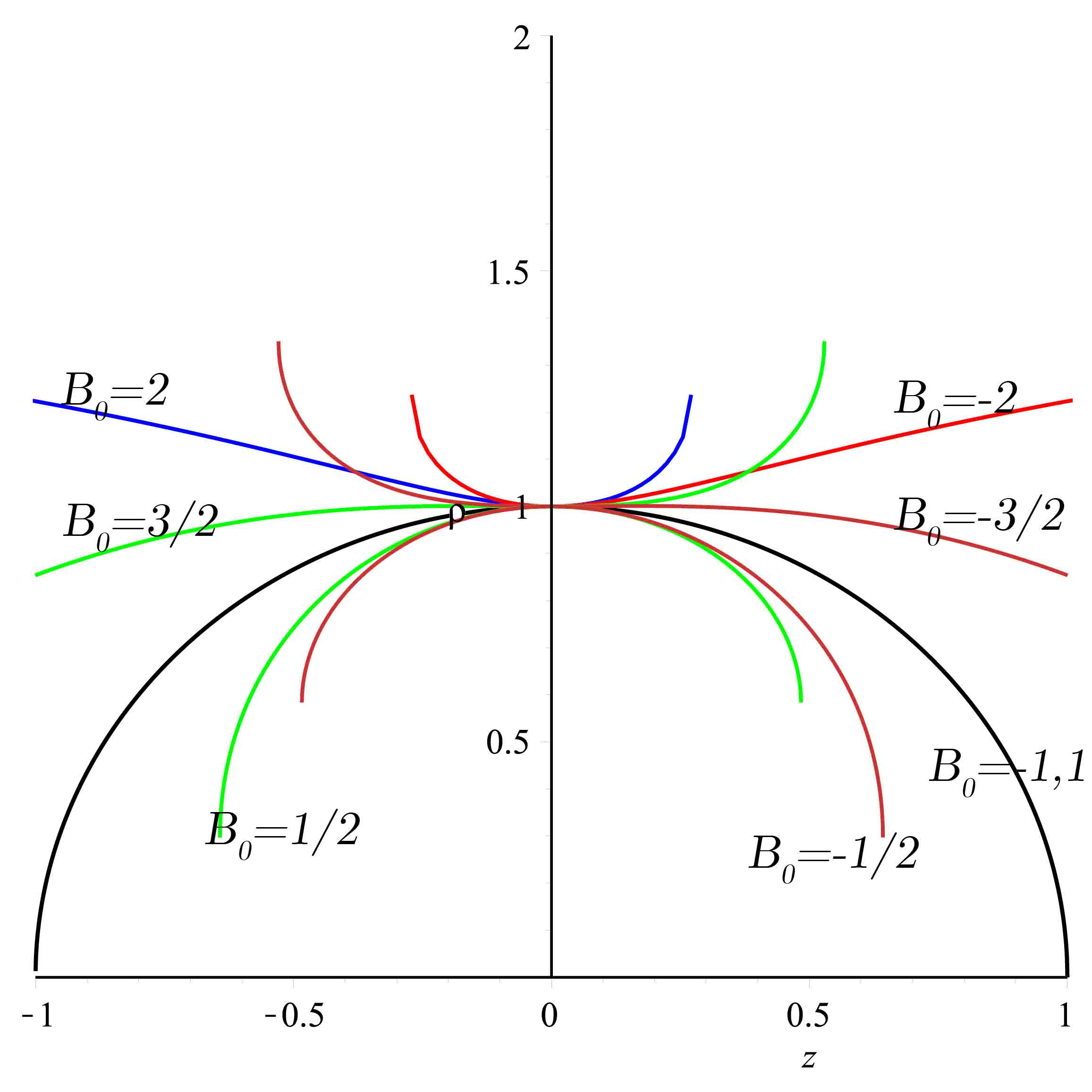
Figure 1: Plotting of $\rho\left(z\right)$ versus $z$ in accordance with the geodesics equation (45), for specific values of $B_{0}$ ($\lambda_{0}=1$). The initial conditions are chosen such that $\rho\left(0\right)=1$ and $\rho^{\prime}\left(0\right)=0.$

III.1 Geodesic Motion in $z=0$ plane for $B_{0}=\lambda_{0}$

As we have shown above the plane $z=0$ has no singularity if $0\leq\frac{B_{0}}{\lambda_{0}}\leq 1$. This makes it to be distinguished from the other planes $z=z_{0}\neq 0.$ Setting $\frac{B_{0}}{\lambda_{0}}=1$ is also the only value in this interval which makes the power of $\rho$ integer. Therefore, we are interested to consider the geodesic motion of a massive particle with unit mass in this spacetime i.e.

$$ds^{2}=-\frac{\lambda_{0}^{2}\left(\rho^{2}+1\right)^{2}}{4}dt^{2}+\\ \frac{\lambda_{0}^{2}\left(\rho^{2}+1\right)^{2}}{4\rho^{2}}d\rho^{2}+\frac{4}{\lambda_{0}^{2}}\frac{\rho^{2}}{\left(\rho^{2}+1\right)^{2}}d\varphi^{2}.$$ (48)

The Lagrangian is given by

$$\mathcal{L}=-\frac{\lambda_{0}^{2}\left(\rho^{2}+1\right)^{2}}{8}\dot{t}^{2}+\\ \frac{\lambda_{0}^{2}\left(\rho^{2}+1\right)^{2}}{8\rho^{2}}\dot{\rho}^{2}+\frac{2}{\lambda_{0}^{2}}\frac{\rho^{2}}{\left(\rho^{2}+1\right)^{2}}\dot{\varphi}^{2},$$ (49)

in which an over dot shows derivative wrt the affine parameter $\lambda$. The conservation of energy and angular momentum is obvious such that

$$\frac{\partial\mathcal{L}}{\partial\dot{t}}=-\frac{\lambda_{0}^{2}\left(\rho^{2}+1\right)^{2}}{4}\dot{t}=-E$$ (50)

and

$$\frac{\partial\mathcal{L}}{\partial\dot{\varphi}}=\frac{4}{\lambda_{0}^{2}}\frac{\rho^{2}}{\left(\rho^{2}+1\right)^{2}}\dot{\varphi}=\ell.$$ (51)

Having $g_{\mu\nu}\frac{dx^{\mu}}{d\lambda}\frac{dx^{\nu}}{d\lambda}=-\epsilon$ where $\epsilon=0$ /$1$ (for unit mass) yields the null or timelike geodesics, implies

$$-\frac{\lambda_{0}^{2}\left(\rho^{2}+1\right)^{2}}{4}\dot{t}^{2}+\frac{\lambda_{0}^{2}\left(\rho^{2}+1\right)^{2}}{4\rho^{2}}\dot{\rho}^{2}+\frac{4}{\lambda_{0}^{2}}\frac{\rho^{2}}{\left(\rho^{2}+1\right)^{2}}\dot{\varphi}^{2}=-\epsilon$$ (52)

or upon using the conserved quantities one finds

$$\dot{\rho}^{2}=\frac{16\rho^{2}E^{2}}{\lambda_{0}^{4}\left(\rho^{2}+1\right)^{4}}-\frac{4\rho^{2}\epsilon}{\lambda_{0}^{2}\left(\rho^{2}+1\right)^{2}}-\ell^{2}.$$ (53)

III.1.1 Radial motion of massive particle

Let’s consider, as the first case, the motion with zero angular momentum of a massive particle i.e., $\ell=0$ and $\epsilon=1.$ These in turn yield

$$\dot{\rho}^{2}=\frac{16\rho^{2}E^{2}}{\lambda_{0}^{4}\left(\rho^{2}+1\right)^{4}}-\frac{4\rho^{2}}{\lambda_{0}^{2}\left(\rho^{2}+1\right)^{2}}$$ (54)

which after getting help from

$$\dot{\rho}^{2}=\left(\frac{\partial\rho}{\partial\lambda}\right)^{2}=\left(\frac{\partial\rho}{\partial t}\right)^{2}\left(\frac{\partial t}{\partial\lambda}\right)^{2}=\left(\frac{\partial\rho}{\partial t}\right)^{2}\frac{16E^{2}}{\lambda_{0}^{4}\left(\rho^{2}+1\right)^{4}}$$ (55)

one finds

$$\left(\frac{\partial\rho}{\partial t}\right)^{2}=\rho^{2}-\frac{\lambda_{0}^{2}\rho^{2}\left(\rho^{2}+1\right)^{2}}{4E^{2}}.$$ (56)

Nevertheless, one may set the affine parameter to be the proper time $\tau$ and therefore

$$\left(\frac{\partial\rho}{\partial\tau}\right)^{2}=\frac{16\rho^{2}E^{2}}{\lambda_{0}^{4}\left(\rho^{2}+1\right)^{4}}-\frac{4\rho^{2}}{\lambda_{0}^{2}\left(\rho^{2}+1\right)^{2}}.$$ (57)

Now suppose the particle starts from rest at $\rho=\rho_{0}$ where $\frac{\partial\rho}{\partial t}=$ $\frac{\partial\rho}{\partial\tau}=0,$ which gives

$$E^{2}=\frac{\lambda_{0}^{2}\left(\rho_{0}^{2}+1\right)^{2}}{4}.$$ (58)

Hence the equations of motion become

$$\left(\frac{\partial\rho}{\partial t}\right)^{2}=\rho^{2}-\frac{\rho^{2}\left(\rho^{2}+1\right)^{2}}{\left(\rho_{0}^{2}+1\right)^{2}}$$ (59)

and

$$\left(\frac{\partial\rho}{\partial\tau}\right)^{2}=\frac{4\rho^{2}\left(\rho_{0}^{2}+1\right)^{2}}{\lambda_{0}^{2}\left(\rho^{2}+1\right)^{4}}-\frac{4\rho^{2}}{\lambda_{0}^{2}\left(\rho^{2}+1\right)^{2}}.$$ (60)

In Fig. 2 we plot $\rho$ versus $t$ (a) and $\tau$ (b). It is very much clear that the motion is periodic which means that the particle is attracted by the origin and while approaches the origin it gains energy and this energy causes to pass the origin and in the other direction slows down to rest and in the same way repeats the motion. The different between the period of motion measured by an observer on the particle and observer in the lab is also manifested in the figures.

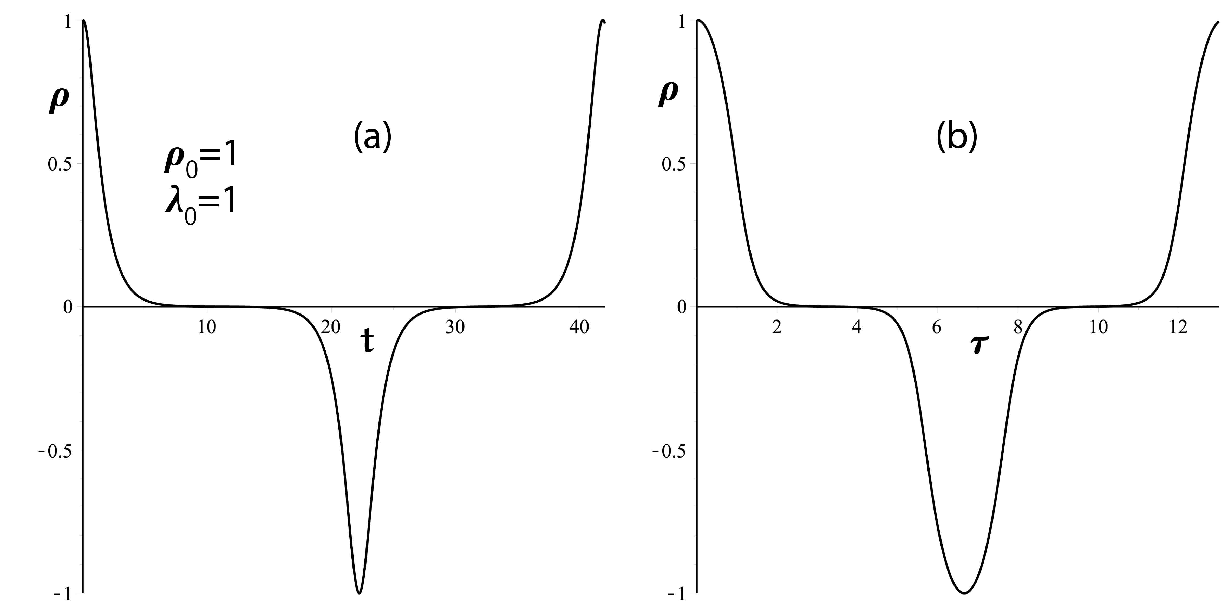
Figure 2: Radial fall from $\rho=1$ through $\rho=0$ (in the $z=0$ plane) for a fixed angle as a function of the coordinate time (Fig. 2a) / proper time (Fig. 2b). The particle crosses $\rho=0$ freely since $\rho=0=z$ is not singular in the chosen interval $\frac{B_{0}}{\lambda_{0}}=1$.

III.1.2 Radial motion of a massless particles

In the same way one may study the motion of a null particle with $\epsilon=0$ and $\ell=0.$ The equation of motion Eq. (53) then reads

$$\dot{\rho}^{2}=\frac{16\rho^{2}E^{2}}{\lambda_{0}^{4}\left(\rho^{2}+1\right)^{4}}$$ (61)

which after using the chain rule we find

$$\left(\frac{d\rho}{dt}\right)^{2}=\rho^{2}.$$ (62)

whose explicit solution is given by

$$\rho=\rho_{0}e^{\pm t}$$ (63)

where $\pm$ refers to the direction of motion.

III.1.3 Circular Motion

To work out the circular motion of a particle on the plane $z=0$ we use the chain rule in (53) to find

$$\left(\frac{d\rho}{d\varphi}\right)^{2}=\\ \frac{16^{2}\rho^{6}E^{2}}{\lambda_{0}^{8}\left(\rho^{2}+1\right)^{8}\ell^{2}}-\frac{64\rho^{6}\epsilon}{\lambda_{0}^{6}\left(\rho^{2}+1\right)^{6}\ell^{2}}-\frac{16\rho^{4}}{\lambda_{0}^{4}\left(\rho^{2}+1\right)^{4}}.$$ (64)

As usual we introduce $u=\frac{1}{\rho}$ to change the equation of motion in the form of

$$\left(\frac{du}{d\varphi}\right)^{2}=\frac{256u^{14}E^{2}}{\lambda_{0}^{8}\left(u^{2}+1\right)^{8}\ell^{2}}-\\ \frac{64u^{10}\epsilon}{\lambda_{0}^{6}\left(u^{2}+1\right)^{6}\ell^{2}}-\frac{16u^{8}}{\lambda_{0}^{4}\left(u^{2}+1\right)^{4}}=A\left(u\right)$$ (65)

Having a photon ($\epsilon=0$) or a massive particle ($\epsilon=1$) moving on a circular orbit means $\left.A\left(u\right)\right|_{u_{c}}=0$ and having an equilibrium path needs an additional condition $\left.\frac{dA\left(u\right)}{du}\right|_{u_{c}}=0.$ Herein $\rho_{c}=\frac{1}{u_{c}}$is the radius of the equilibrium circular orbit. For the massive particle ($\epsilon=1$) these conditions yield

$$E^{2}=\frac{\left(u_{c}^{2}-1\right)\left(u_{c}^{2}+1\right)^{2}\lambda_{0}^{2}}{4\left(u_{c}^{2}-3\right)u_{c}^{4}}$$ (66)

and

$$\ell^{2}=\frac{8u_{c}^{2}}{\lambda_{0}^{2}\left(u_{c}^{2}+1\right)^{2}\left(u_{c}^{2}-3\right)}$$ (67)

and therefore the radius of the circular path is found to be the positive root of the following equation

$$\left(u_{c}^{4}-1\right)\left(u_{c}^{2}+1\right)^{4}=\frac{32E^{2}}{\lambda_{0}^{4}\ell^{2}}u_{c}^{6}.$$ (68)

From the latter equation we see that for $E=0$ a circular path with $u_{c}=1$ is possible. This is in fact the maximum value of the possible radius for a circular motion. Particles with higher energy may be able to orbit about the origin with a radius less then one.

For a massless particle the same conditions dictate a single circular path with

$$u_{c}=\sqrt{3}$$ (69)

and energy satisfying

$$\frac{E^{2}}{\ell^{2}}=\frac{16}{27}\lambda_{0}^{4}.$$ (70)

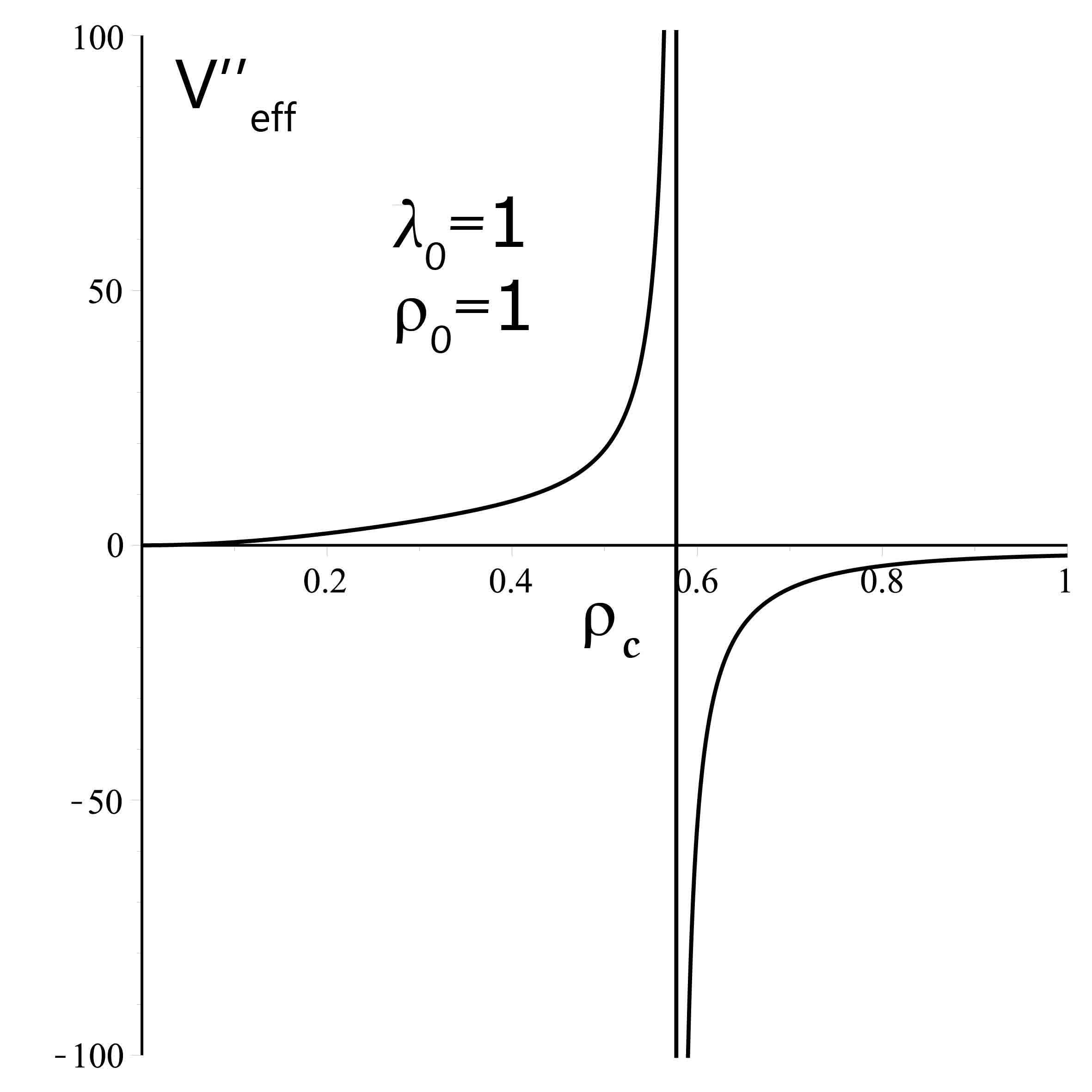
Figure 3: Stability condition for particles in circular orbits. From Eq. (74), $V^{\prime\prime}\left(\rho_{c}\right)$ is plotted versus the circular radius $\rho_{c}.$ It is observed that for $\rho_{c}<\frac{1}{\sqrt{3}}$ we have stable orbits since it gives $V^{\prime\prime}\left(\rho_{c}\right)>0$.

III.1.4 Stability of the circular motion

To see whether the circular path of the particles found above are stable or not we go back to the Eq. (54) and rewrite it in the form of one dimensional motion

$$\frac{1}{2}\left(\frac{d\rho}{d\lambda}\right)^{2}+V_{eff}=0,$$ (71)

$$V_{eff}=-\text{ }\frac{8\rho^{2}E^{2}}{\lambda_{0}^{4}\left(\rho^{2}+1\right)^{4}}+\frac{2\rho^{2}\epsilon}{\lambda_{0}^{2}\left(\rho^{2}+1\right)^{2}}+\frac{\ell^{2}}{2}.$$ (72)

An expansion of $V_{eff}$ about $\rho=\rho_{c}$ yields (we note that at equilibrium circular path both $V_{eff}$ and its first derivative vanish)

$$\left(\frac{dx}{d\lambda}\right)^{2}+V_{eff}^{\prime\prime}\left(\rho_{c}\right)x^{2}=0$$ (73)

where $x=\rho-\rho_{c}$ and

$$V_{eff}^{\prime\prime}\left(\rho_{c}\right)=\frac{16\left(2u_{c}^{4}-3u_{c}^{2}+3\right)u_{c}^{4}}{\left(u_{c}^{2}-3\right)\left(u_{c}^{2}+1\right)^{4}\lambda_{0}^{2}}.$$ (74)

A second derivative wrt $\lambda$ from (71) admits

$$\left(\frac{d^{2}x}{d\lambda^{2}}\right)+V_{eff}^{\prime\prime}\left(\rho_{c}\right)x=0$$ (75)

which has an oscillatory motion of $x$ wrt $\lambda$ (stable motion) if $V_{eff}^{\prime\prime}\left(\rho_{c}\right)>0.$ Fig. 3 displays $V_{eff}^{\prime\prime}\left(\rho_{c}\right)$ versus $\rho_{c}.$ As it is clear those orbits whose radius is less then $\frac{1}{\sqrt{3}}$ are stable. Similar argument can be repeated for the massless particles. The effective potential and its first derivative at $\rho=\rho_{c}=\frac{1}{\sqrt{3}}$ are zero while

$$V_{eff}^{\prime\prime}\left(\rho_{c}\right)=\frac{243E^{2}}{32\lambda_{0}^{4}}$$ (76)

which is clearly positive. Therefore the orbit of a photon is stable which is unlike the Schwarzschild and Reissner-Nordström spacetime.

III.1.5 Null Geodesics in Kundt form

The Lagrangian of an uncharged particle moving in the spacetime identified by (37) reads as

$$L=\dot{u}\dot{v}+H\dot{u}^{2}+e^{2\left(K-U\right)}\left(\dot{\rho}^{2}+\dot{z}^{2}\right)$$ (77)

in which ($\cdot\equiv\frac{d}{d\lambda}$). The first equation $\frac{d}{d\lambda}\left(\frac{\partial L}{\partial\dot{v}}\right)=\frac{\partial L}{\partial v}$ yields

$$\ddot{u}=0$$ (78)

which in turn implies $\dot{u}=$constant. This basically suggests that our affine parameter $\lambda$ is $u.$ The second equation $\frac{d}{d\lambda}\left(\frac{\partial L}{\partial\dot{u}}\right)=\frac{\partial L}{\partial u}$ gives

$$\frac{dv}{du}+2H=\alpha_{0}$$ (79)

where $\alpha_{0}$ is an integration constant. The other two equations are also given by

$$\ddot{\rho}+\left(K-U\right)_{\rho}\left(\dot{\rho}^{2}-\dot{z}^{2}\right)+2\dot{\rho}\dot{z}\left(K-U\right)_{z}=\dot{\rho}U_{\rho}e^{2\left(2U-K\right)}$$ (80)

and

$$\ddot{z}+\left(K-U\right)_{z}\left(\dot{z}^{2}-\dot{\rho}^{2}\right)+2\dot{\rho}\dot{z}\left(K-U\right)_{\rho}=\dot{z}U_{z}e^{2\left(2U-K\right)}$$ (81)

in which herein ($\cdot\equiv\frac{d}{du}$).  For $\varphi=$constant one finds $du=dt,$ and the equation (79) is satisfied if $\alpha_{0}=0$. For null-geodesics we find from (77) that

$$\left(\rho_{u}^{2}+z_{u}^{2}\right)=e^{2\left(2U-K\right)}$$ (82)

and upon the symmetry between $\rho$ and $z$ we set $\rho=\kappa z$ with $\kappa=$constant to get (we choose also $\lambda_{0}=1$)

$$\frac{dz}{e^{2U-K}}=\frac{du}{\sqrt{1+\kappa^{2}}}$$ (83)

in which $du=dt.$ A substitution and integration admits

$$z = \left(\frac{B_{0}^{2}-1}{k_{0}}\left(t-t_{0}\right)\right)^{\frac{1}{B_{0}^{2}-1}}$$

$$\left(B_{0}^{2}\neq 1\right)$$

where $k_{0}=\frac{\kappa^{2B_{0}+B_{0}^{2}}}{\sqrt{1+\kappa^{2}}\left(1+\sqrt{1+\kappa^{2}}\right)^{2B_{0}}}$ and $t_{0}$ is an integration constant. For $B_{0}^{2}=1$ we find

$$k_{0}\ln z=t-t_{0}.$$ (85)

This brief analysis of Kundt’s null geodesics recovers the equivalent results of the previous analysis. Namely, that the exact integrals of geodesics in a section of the ($\rho,z$) plane doesn’t cover the whole plane. We conclude therefore that null geodesic incompleteness remains intact irrespective of the representation of the metric.

IV Conclusion

Being inspired by the superposed solutions in colliding wave spacetimes which unfortunately received no attentions we show here in a similar manner that BR and ML spacetimes can be combined in a single metric. The distinction between the two problems, i.e. colliding waves and axial symmetry, is that in the latter case superposition worked in the more familiar cylindrical $\left(\rho,z\right)$ coordinates rather than the prolate / oblate ones. The obtained metric inherits the imprints of both solutions. It is not conformally flat for instance, and regularity at the origin i.e. at $\rho=z=0,$ holds provided in $0\leq\frac{B_{0}}{\gamma_{0}}\leq 1.$ For an arbitrary ML parameter, however, our solution becomes singular on the symmetry axis. Due to the fractional powers of $\rho$ our solution is neither smooth nor flat on the symmetry axis. Exact solution of geodesics reveals that null geodesics in the singular manifold are not complete whereas BR and ML spacetimes separately are known to admit complete geodesics. One drawback of our solution is that $\gamma_{0}\rightarrow 0$ limit i.e. the ML limit doesn’t exist. In a single coordinate patch the large type-D Einstein-Maxwell family of Plebanski and Demianski (PD) also suffers a similar problem. In this regard our overall impression is that our non-smooth solution doesn’t belong to the class of PD. Finally we add that this simple example may serve to pave the way for further ’superposed’ spacetimes in general relativity, including the higher dimensional ones.

- (1) B. Bertotti, Phys. Rev. 116, 1331 (1959); I. Robinson, Bull. Acad. Pol. Sci. Ser. Sci. Math. Astr. Phys. 7, 351 (1959).
- (2) M. A. Melvin, Phys. Letters 8, 65 (1964). W. B. Bonnor, Proc. Phys. Soc. A 67, 225 (1954).
- (3) D. Garfinkle and E. N. Glass, Class. Quantum Grav. 28, 215012 (2011).
- (4) W. Kundt, Proc. Roy. Soc. A 270, 328 (1962).
- (5) J. F. Plebanski and M. Demiahski, Rotating, charged, and uniformly accelerating mass in general relativity, Ann. Phys. 98, 98 (1976); J. Plebański, J. Math. Phys. 20, 1946 (1979); J. B. Griffiths and J. Podolský, Int. J. Mod. Phys. D 15, 335 (2006).
- (6) J. B. Griffiths and J. Podolský, ”Exact Space-Times in Einstein’s General Relativity”, Cambridge Monographs on Mathematical Physics, Cambridge University Press, Cambridge U.K. (2009).
- (7) S. Chandrasekhar and B. C. Xanthopoulos Proc. Roy. Soc. A 140, 311 (1987).
- (8) P. Bell and P. Szekeres, Gen. Rel. Grav. 5, 275 (1974).
- (9) K. A. Khan and R. Penrose, Nature, 229, 185 (1971).
- (10) M. Halilsoy, J. Math. Phys. 34, 3553 (1993).
- (11) M. Halilsoy, Gen. Rel. Grav. 25, 275 (1992).
- (12) M. Halilsoy, J. Math. Phys. 33, 4225 (1992).
- (13) D. M. Zipoy, J. Math. Phys. 7, 1137 (1966) B. H. Voorhees, Phys. Rev. D. 2, 2119 (1970).
- (14) R. Gautreau and J. L. Anderson, Phys. Lett. A 25, 291 (967).