Matching lattice and continuum axial-vector and vector currents with NRQCD and HISQ quarks

Abstract

We match the continuum and lattice axial-vector and vector currents at one loop in perturbation theory. For the heavy quarks we use the nonrelativistic QCD (NRQCD) action and for the light quarks the Highly Improved Staggered Quark (HISQ) action. We present results for both massless and massive HISQ quarks and as part of the matching procedure we include a discussion of the one loop HISQ renormalisation parameters.

I Introduction

Electroweak processes are an important tool in understanding the Standard Model (SM) of particle physics, serving as an input into tests of the unitarity of the Cabibbo-Kobayashi-Maskawa (CKM) matrix and as a probe for new physics. The hadronic matrix elements that characterise the strong interaction dynamics of these processes are a crucial ingredient in the determination of CKM unitarity.

Global fits to the CKM unitarity have, in recent years, indicated some tensions at the 2-3$\sigma$ level within the SM E. Lunghi and A. Soni (2011a, b); J. Laiho et al. (2010, 2012). In many cases, the constraints on the CKM unitarity triangle are limited by the precision with which the nonperturbative inputs are known and thus it is imperative that these inputs are determined as precisely as possible.

The HPQCD collaboration has undertaken a suite of precision calculations of heavy-light mesons as part of a program to precisely determine nonperturbative contributions to electroweak parameters. Recent calculations of the decay constants $f_{B}$ and $f_{B_{s}}$ have achieved a precision at the $2\%$ level, by taking advantage of the small discretisation errors and good chiral properties of the Highly Improved Staggered Quark (HISQ) action C. McNeile et al. (2012); H. Na et al. (2012). These results represent the most precise currently available for these decay constants. In addition, nonperturbative studies of the heavy-light semileptonic decays $B\rightarrow\pi\ell\nu$, $B\rightarrow K\ell^{+}\ell^{-}$ and $B_{s}\rightarrow K\ell\nu$ are underway C. Bouchard (2012).

The work of Ref. H. Na et al. (2012) and C. Bouchard (2012) use HISQ light quarks and the nonrelativistic QCD (NRQCD) action for the heavy quarks. These calculations require matching the heavy-light axial-vector and vector currents in the effective theory on the lattice with full QCD. In this article we report on the one loop perturbative matching of the HISQ-NRQCD axial-vector and vector current matching for both massless and massive HISQ quarks. As part of this procedure we determine the mass and wavefunction renormalisation for massive HISQ quarks. Our matching results for massive HISQ quarks will be relevant for future studies of heavy-heavy decays $B_{(s)}\rightarrow D_{(s)}\ell\nu$.

In the next section we describe the quark and gluon actions used in our calculation. We then review the formalism for extracting renormalisation parameters from relativistic lattice actions and apply these procedures to first massless and then massive HISQ quarks. We include results for the one loop NRQCD mass and wavefunction renormalisation in Section III.5. In Section IV we outline the calculation of the matching coefficients and then, in Section V, we present our results for a range of heavy quark masses. We conclude with a summary in Section VI.

II The Lattice Actions

II.1 Gluon Action

We use the Symanzik improved gluon action with tree level coefficients P. Weisz (1983); P. Weisz and R. Wohlert (1984); G. Curci et al. (1983); M. Luescher and P. Weisz (1985), given by

$$S_{G}=-\frac{\beta}{3u_{0}^{4}}\sum_{x,\mu>\nu}\left[5P_{\mu\nu}-\frac{1}{4u_{0}^{2}}\left(R_{\mu\nu}+R_{\nu\mu}\right)\right].$$ (1)

Here $P_{\mu\nu}$ is the plaquette,

$$P_{\mu\nu}=\frac{1}{N_{c}}\text{Re}\text{Tr}\Big{\{}U_{\mu}(x)U_{\nu}(x+\hat{\mu})U_{\mu}^{\dagger}(x+\hat{\nu})U_{\nu}^{\dagger}(x)\Big{\}},$$ (2)

and $R_{\mu\nu}$ the six-link loop,

$$R_{\mu\nu}={} \frac{1}{N_{c}}\text{Re}\text{Tr}\Big{\{}U_{\mu}(x)U_{\mu}(x+\hat{\mu})U_{\nu}(x+2\hat{\mu})$$

$$\times U_{\mu}^{\dagger}(x+\hat{\mu}+\hat{\nu})U_{\mu}^{\dagger}(x+\hat{\nu})U_{\nu}^{\dagger}(x)\Big{\}},$$ (3)

with $\beta=2N_{c}/g^{2}$ and $u_{0}$ the tadpole improvement factor G.P. Lepage and P.B. Mackenzie (1993). Radiative improvements to the gluon action do not contribute to the one loop matching calculation. In general, radiative improvement generates an ${\cal O}(\alpha_{s})$ insertion in the gluon propagator. There are no external gluons in our calculation, so any such improvements only contribute at two loops and higher.

We include a gauge-fixing term

$$S_{\xi}=\frac{1}{2\xi}\sum_{x}\left[\sum_{\mu}\Delta_{\mu}(aA_{\mu})\right]^{2},$$ (4)

where $\Delta_{\mu}$ is the symmetrised difference operator, which acts on the gauge fields as

$$\Delta_{\mu}A_{\mu}(x)\equiv A_{\mu}\left(x+\frac{\hat{\mu}}{2}\right)-A_{\mu}\left(x-\frac{\hat{\mu}}{2}\right),$$ (5)

and $\xi$ is the gauge parameter. Where possible, we confirm that gauge invariant quantities are independent of the choice of gauge parameter by working in both Feynman, $\xi=1$, and Landau, $\xi=0$, gauges.

II.2 Light Quark Action

We discretise the light quarks in this work using the Highly Improved Staggered Quark (HISQ) action E. Follana et al. (2007). The HISQ action significantly reduces taste breaking discretization errors and has been used successfully to simulate both $b$ and $c$ quark systems E. Follana et al. (2008); C. McNeile et al. (2010); E.B. Gregory et al. (2011); R.J. Dowdall et al. (2012a). There are two equivalent methods for writing staggered quark actions, using either four component “naive” fermions or one component “staggered” fields G.P. Lepage (1999); M. Wingate et al. (2003). Throughout this calculation we use the naive fermion representation and we denote the bare quark mass $am_{0}$. In Section III.4.1 we present our results for massless HISQ quarks, corresponding to $am_{0}=0$. Before we present the quark actions used in this work, we pause to briefly discuss some notation, which we summarise in Table 1.

Table 1: Summary of quark mass notation.

HISQ	$am_{0}$	bare light quark mass
	$am_{\text{tree}}$	tree level pole mass
	$am_{1}$	one loop pole mass
	$am_{\text{kin}}$	kinetic mass
NRQCD	$aM_{0}$	bare heavy quark mass

We use four different quark mass definitions for relativistic HISQ quarks: the bare quark mass; the tree level and one loop pole masses, $am_{\text{tree}}$ and $am_{1}$ respectively; and the kinetic mass, $am_{\text{kin}}$. We distinguish these relativistic quark masses from the nonrelativistic quark mass in NRQCD by using a lowercase $m$ for HISQ quarks and an uppercase $M$ for NRQCD quarks. Only the bare heavy quark mass $aM_{0}$ is required for nonrelativistic quarks in this calculation.

The starting point for constructing the HISQ action is the AsqTad action G.P. Lepage (1999), which is given by

$$S_{\text{AsqTad}}=a^{4}\sum_{x}\overline{\psi}(x)\left(\gamma_{\mu}\nabla_{\mu}^{\text{AsqTad}}+m_{0}\right)\psi(x),$$ (6)

where the AsqTad operator is

$$\nabla_{\mu}^{\text{AsqTad}}=\nabla_{\mu}^{F}-\frac{a^{2}}{6}(\nabla_{\mu})^{3}.$$ (7)

Here the three-link term $(\nabla_{\mu})^{3}$ is referred to as the “Naik” term and the superscript $F$ indicates that we use fattened links in the lattice difference operator $\nabla_{\mu}$. The fattened links are given by

$$U_{\mu}(x)\rightarrow{\cal F}_{\mu}^{\text{AsqTad}}U_{\mu}(x),$$ (8)

where

$${\cal F}_{\mu}^{\text{AsqTad}}={} \left[{\cal F}_{\mu}-\sum_{\rho\neq\mu}\frac{a^{2}(\nabla_{\rho})^{2}}{4}\right],$$ (9)

$${\cal F}_{\mu}={} \prod_{\rho\neq\mu}\left(1+\frac{a^{2}\nabla_{\rho}^{(2)}}{4}\right)_{\text{symmetrised}}.$$ (10)

The second term in Equation (9) is the so-called “Lepage” term. The difference operator acts on fermion fields as

$$\nabla_{\mu}\psi(x)=\frac{1}{2a}\left[U_{\mu}(x)\psi(x+\hat{\mu})-U_{\mu}^{\dagger}(x-\hat{\mu})\psi(x-\hat{\mu})\right],$$ (11)

whilst the discretised derivatives acting on link variables are, for $\mu\neq\nu$,

$$\nabla_{\mu}U_{\nu}(x)={} \frac{1}{2}\Big{[}U_{\mu}(x)U_{\nu}(x+\hat{\mu})U_{\mu}^{\dagger}(x+\hat{\nu})$$

$$-U_{\mu}^{\dagger}(x-\hat{\mu})U_{\nu}(x-\hat{\mu})U_{\mu}(x-\hat{\mu}+\hat{\nu})\Big{]},$$ (12)

$$\nabla_{\mu}^{(2)}U_{\nu}(x)={} \Big{[}U_{\mu}(x)U_{\nu}(x+\hat{\mu})U_{\mu}^{\dagger}(x+\hat{\nu})-2U_{\nu}(x)$$

$$+U_{\mu}^{\dagger}(x-\hat{\mu})U_{\nu}(x-\hat{\mu})U_{\mu}(x-\hat{\mu}+\hat{\nu})\Big{]}.$$ (13)

The HISQ action is an extension of the AsqTad action that includes two levels of link fattening and a tuned coefficient for the Naik term. Whilst the AsqTad action has negligible tree level errors for light quarks, this is not true for charm or bottom quarks E. Follana et al. (2007). Charm quarks are generally nonrelativistic in typical mesons, so the rest energy of the quark is much larger than its momentum. The dominant tree level errors are therefore ${\cal O}(a^{4}m_{0}^{4})$. One suppresses these errors by tuning the coefficient of the Naik term

$$\frac{a^{2}}{6}(\nabla_{\mu})^{3}\rightarrow\frac{a^{2}}{6}(1+\epsilon)(\nabla_{\mu})^{3}.$$ (14)

One also adds a second level of fattening in the link variables to reduce the discretisation errors arising from taste exchange interactions in the HISQ action. Between the smearing operations, one sandwiches a reunitarisation operator, ${\cal U}$, that projects the smeared link variables back to $SU(3)$ or $U(3)$. For simplicity, the Lepage term is included in the HISQ action only after the second level of link fattening. The resulting action is

$$S_{\text{HISQ}}=a^{4}\sum_{x}\overline{\psi}(x)\left(\gamma_{\mu}\nabla_{\mu}^{\text{HISQ}}+m_{0}\right)\psi(x),$$ (15)

where

$$\nabla_{\mu}^{\text{HISQ}}=\nabla_{\mu}^{(FUF)}-\frac{a^{2}}{6}(1+\epsilon)\left(\nabla_{\mu}^{(UF)}\right)^{3}.$$ (16)

The superscripts indicate that the first operator, $\nabla_{\mu}^{(FUF)}$, is built from the full HISQ-smeared links, given by

$${\cal F}_{\mu}^{\text{HISQ}}=\left({\cal F}_{\mu}-\sum_{\rho\neq\mu}\frac{a^{2}(\nabla_{\rho})^{2}}{2}\right){\cal U}{\cal F}_{\mu},$$ (17)

whilst the second operator, $\nabla_{\mu}^{(UF)}$, uses only one level of smearing:

$$\nabla_{\mu}^{(UF)}={\cal U}{\cal F}_{\mu}.$$ (18)

We define the operator ${\cal F}_{\mu}$ in Equation (10).

We give results for both massless and massive HISQ quarks. For massless quarks the tuning parameter is just $\epsilon=0$. For massive quarks we set the tuning parameter to its tree level value, $\epsilon=\epsilon_{\text{tree}}$, for consistency with non-perturbative simulations H. Na et al. (2012). We discuss this in more detail in Section III.4.

II.3 Heavy Quark Action

For the heavy quark fields, $\psi(\mathbf{x},t)$, we use the NRQCD action of A. Gray et al. (2005); R.J. Dowdall et al. (2012b), which is improved through ${\cal O}(1/M_{0}^{2})$ and ${\cal O}(a^{2})$ and includes the leading relativistic ${\cal O}(1/M_{0}^{3})$ correction. The NRQCD action is

$$S_{\text{NRQCD}}={} \sum_{\mathbf{x},t}\psi^{\dagger}_{t}\psi_{t}-\psi^{\dagger}_{t}\left(1-\frac{a\delta H}{2}\right)\left(1-\frac{aH_{0}}{2n}\right)^{n}$$

$$\times U_{4}^{\dagger}\left(1-\frac{aH_{0}}{2n}\right)^{n}\left(1-\frac{a\delta H}{2}\right)\psi_{t-1},$$ (19)

where $\psi^{\dagger}_{t}=\psi^{\dagger}(\mathbf{x},t)$ and $\psi_{t-1}=\psi(\mathbf{x},t-1)$.

Here the leading kinetic term in the NRQCD action is given by

$$aH_{0}=-\frac{\Delta^{(2)}}{2aM_{0}},$$ (20)

and the correction terms are

$$a\delta H={} -c_{1}\frac{(\Delta^{(2)})^{2}}{8(aM_{0})^{3}}+c_{2}\frac{i}{8(aM_{0})^{2}}\left(\nabla\cdot\widetilde{\mathbf{E}}-\widetilde{\mathbf{E}}\cdot\nabla\right)$$

$$-c_{3}\frac{1}{8(aM_{0})^{2}}\sigma\cdot\left(\widetilde{\nabla}\times\widetilde{\mathbf{E}}-\widetilde{\mathbf{E}}\times\widetilde{\nabla}\right)$$

$$-c_{4}\frac{1}{2aM_{0}}\sigma\cdot\widetilde{\mathbf{B}}+c_{5}\frac{\Delta^{(4)}}{24aM_{0}}-c_{6}\frac{(\Delta^{(2)})^{2}}{16n(aM_{0})^{2}}.$$ (21)

All the derivatives are tadpole improved and the discretised difference operators are

$$\Delta^{(2)}=\sum_{j=1}^{2}\nabla_{j}^{(2)},\quad\Delta^{(4)}=\sum_{j=1}^{3}\nabla_{j}^{(4)},\quad\widetilde{\nabla}_{i}=\nabla_{i}-\frac{1}{6}\nabla_{i}^{(3)},$$ (22)

where the improved operators act on fermion fields via

$$\nabla_{\mu}^{(2)}\psi(x)={} U_{\mu}(x)\psi(x+\hat{\mu})$$

$$+U^{\dagger}_{\mu}(x-\hat{\mu})\psi(x-\hat{\mu})-2\psi(x),$$ (23)

$$\nabla_{\mu}^{(3)}\psi(x)={} \frac{1}{2}\bigg{[}U_{\mu}(x)U_{\mu}(x+\hat{\mu})\psi(x+2\hat{\mu})$$

$$-U^{\dagger}_{\mu}(x-\hat{\mu})U^{\dagger}_{\mu}(x-2\hat{\mu})\psi(x-2\hat{\mu})\bigg{]}$$

$$-U_{\mu}(x)\psi(x+\hat{\mu})+U^{\dagger}_{\mu}(x-\hat{\mu})\psi(x-\hat{\mu}),$$ (24)

$$\nabla_{\mu}^{(4)}\psi(x)={} U_{\mu}(x)U_{\mu}(x+\hat{\mu})\psi(x+2\hat{\mu}),$$

$$+U^{\dagger}_{\mu}(x-\hat{\mu})U^{\dagger}_{\mu}(x-2\hat{\mu})\psi(x-2\hat{\mu})+6\psi(x)$$

$$-4\Big{(}U_{\mu}(x)\psi(x+\hat{\mu})+U^{\dagger}_{\mu}(x-\hat{\mu})\psi(x-\hat{\mu})\Big{)}.$$ (25)

The improved chromo-electric and -magnetic fields, $\widetilde{E}_{j}=\widetilde{F}_{i4}$ and $\widetilde{B}_{j}=-\epsilon_{ijk}\widetilde{F}_{jk}/2$, are defined in terms of the improved field strength tensor, given by M. Wingate et al. (2003):

$$\widetilde{F}_{\mu\nu}={} \frac{5}{3}F_{\mu\nu}(x)-\frac{1}{6}\bigg{(}U_{\mu}(x)F_{\mu\nu}(x+\hat{\mu})U^{\dagger}_{\mu}(x)$$

$$+U^{\dagger}_{\mu}(x-\hat{\mu})F_{\mu\nu}(x-\hat{\mu})U_{\mu}(x-\hat{\mu})-(\mu\leftrightarrow\nu)\bigg{)},$$ (26)

where

$$F_{\mu\nu}(x)={} -\frac{i}{2g}\left(\Omega_{\mu\nu}(x)-\Omega_{\mu\nu}^{\dagger}(x)\right),$$ (27)

$$\Omega_{\mu\nu}(x)={} \frac{1}{4}\sum_{\{(\alpha,\beta)\}}U_{\alpha}(x)U_{\beta}(x+\hat{\alpha})$$

$$\times U_{-\alpha}(x+\hat{\alpha}+\hat{\beta})U_{-\beta}(x+\hat{\beta}).$$ (28)

The final sum runs over

$$\{(\alpha,\beta)\}=\{(\mu,\nu),(\nu,-\mu),(-\mu,-\nu),(-\nu,\mu)\},$$ (29)

with $\mu\neq\nu$.

The values of the coefficients, $c_{i}$, in the NRQCD action are fixed by matching lattice NRQCD to full QCD. We use the tree level values of $c_{i}=1$ for all $i=1,\,\cdots,6$, and do not consider the effects of radiative improvement of the NRQCD action.

III Quark self energy

Perturbative calculations of the self energy for massless AsqTad quarks were carried out in E. Gulez et al. (2004) as part of the matching calculation for NRQCD-AsqTad currents. In this work, we extend these results to HISQ fermions. We update the results for the massless case and generalise the results to massive quarks, applying the methods of S. Groote and J. Shigemitsu (2000) to extract the self energy parameters.

III.1 HISQ Parameters

The general formalism for self energy calculations is laid out in B.P.G. Mertens et al. (1998) and developed in S. Groote and J. Shigemitsu (2000). In this section we apply this formalism to the HISQ action, concentrating on the massive case.

We start with the quark two-point correlation function,

$$\langle\psi(t,\mathbf{p}^{\prime})\overline{\psi}(0,\mathbf{p})\rangle=(2\pi)^{3}\delta(\mathbf{p}-\mathbf{p}^{\prime})G(t,\mathbf{p}),$$ (30)

which defines the quark propagator $G(t,\mathbf{p})$. The bare quark field $\overline{\psi}(0,\mathbf{p})$ creates multiparticle states in addition to a one-quark state and so one expects the quark propagator to take the form

$$G(t,\mathbf{p})={\cal Z}_{2}(\mathbf{p})e^{-E(\mathbf{p})t}\Gamma_{\text{proj}}+\cdots.$$ (31)

Here $\Gamma_{\text{proj}}$ is a projection operator in Dirac space; the ellipses represent multiparticle states and lattice artifacts, which we will not consider any further; and ${\cal Z}_{2}(\mathbf{p})$ is the single quark residue.

The use of a lattice regulator distorts the mass shell of the quark, which would otherwise satisfy the relativistic dispersion relation in Euclidean space. To account for the distorted pole position in a systematic manner, one therefore defines the rest mass of the quark, $m_{Q}$, as

$$m_{Q}=E(\mathbf{p}=\mathbf{0})$$ (32)

and the wavefunction renormalisation as

$$Z_{Q}={\cal Z}_{2}(\mathbf{p}=\mathbf{0}).$$ (33)

In Sections III.4.1 and III.4.2 we will use $Z_{q}$ and $Z_{Q}$ to denote the massless and massive wavefunction renormalisations respectively; in this section, however, we use $Z_{Q}$ as shorthand for either $Z_{q}$ or $Z_{Q}$ for notational simplicity.

We renormalise at the point $(p_{0},\mathbf{p})=(iE,\mathbf{0})$ and therefore consider a zero spatial momentum quark propagating forward in time, for which one expects

$$G(t,\mathbf{0})=Z_{Q}e^{-Et}\frac{1+\gamma_{0}}{2}+\cdots.$$ (34)

We denote the momentum space quark propagators for the full and free theories $G(p)$ and $G_{0}(p)$ respectively. These propagators are related via the quark self energy, $\Sigma(p)$:

$$G^{-1}(p)=G_{0}^{-1}(p)-\Sigma(p),$$ (35)

where the self energy is the sum of all one-particle irreducible graphs; in perturbation theory one assumes that the self energy is a “small” correction. The pole corresponding to the single particle quark state has a nonzero residue in the limit that the self energy vanishes, whilst the residues of the multiparticle states vanish in the absence of an interaction.

Carrying out the Fourier transform in $p_{0}$ of the full quark propagator, $G(p)$, one finds

$$G(t,\mathbf{p})=\int_{-\pi/a}^{\pi/a}\frac{\text{d}p_{0}}{2\pi}e^{-ip_{0}t}G(p_{0},\mathbf{p}).$$ (36)

We identify this expression at zero spatial momentum with Equation (34), which enables us to relate the mass and wavefunction renormalisation to parameters in the action, via the quark propagator. In the following derivations, we will neglect factors of the lattice spacing $a$ for simplicity. These can be easily included at the end of the derivations by dimensional analysis.

III.2 Pole mass

For HISQ fermions, the form of the free propagator is

$$G_{0}^{-1}(p)=\sum_{\mu}i\gamma_{\mu}\sin\left(p_{\mu}\right)K_{\mu}(p)+m_{0}.$$ (37)

Here $m_{0}$ is the bare quark mass and

$$K_{\mu}(p)=1+\frac{1+\epsilon}{6}\left(\sin p_{\mu}\right)^{2}.$$ (38)

We write the one loop self energy as

$$\Sigma^{(1)}(p)=\sum_{\mu}i\gamma_{\mu}\sin\left(p_{\mu}\right)\Sigma^{(p\!\!\!/)}_{\mu}(p)+\Sigma^{(\mathbb{I})}(p)\mathbb{I},$$ (39)

where $\mathbb{I}$ is the identity element of the Clifford algebra, so that the one loop propagator is

$$G(p)=\frac{-\sum_{\mu}i\gamma_{\mu}\sin\left(p_{\mu}\right)\left[K_{\mu}(p)-\alpha_{s}\Sigma^{(p\!\!\!/)}_{\mu}(p)\right]+m_{0}-\alpha_{s}\Sigma^{(\mathbb{I})}(p)}{\sum_{\rho}\left(\sin\left(p_{\rho}\right)\right)^{2}\left[K_{\rho}(p)-\alpha_{s}\Sigma^{(p\!\!\!/)}_{\rho}(p)\right]^{2}+\left[m_{0}-\alpha_{s}\Sigma^{(\mathbb{I})}(p)\right]^{2}}.$$ (40)

At zero spatial momentum the pole condition for the forward propagating quark is

$$\sinh(E)\left(1-\frac{1+\epsilon}{6}\left(\sinh(E)\right)^{2}-\alpha_{s}\Sigma^{(p\!\!\!/)}_{0}\right)=m_{0}-\alpha_{s}\Sigma^{(\mathbb{I})},$$ (41)

where we have neglected the arguments of $\Sigma^{(p\!\!\!/)}$ and $\Sigma^{(\mathbb{I})}$ for clarity. We now expand the quark energy and tuning parameter $\epsilon$ to one loop as

$$E={} m_{\text{tree}}+\alpha_{s}m_{1},$$ (42)

$$\epsilon={} \epsilon_{\text{tree}}+\alpha_{s}\epsilon_{1}.$$ (43)

Substituting these expressions into the pole condition, Equation (41), gives an expression for the tree level pole mass, $m_{\text{tree}}$, at fixed bare mass, $m_{0}$:

$$\sinh(m_{\text{tree}})\left[1-\frac{1+\epsilon_{\text{tree}}}{6}\left(\sinh(m_{\text{tree}})\right)^{2}\right]=m_{0}.$$ (44)

We then fix $\epsilon_{\text{tree}}$ by requiring that the tree level pole mass is equal to the tree level kinetic mass. We discuss this condition in more detail in Appendix A. One ultimately finds

$$\epsilon_{\text{tree}}={} -1+\frac{1}{\left(\sinh(m_{\text{tree}})\right)^{2}}$$

$$\times\left[4-\sqrt{4+\frac{12m_{\text{tree}}}{\cosh(m_{\text{tree}})\sinh(m_{\text{tree}})}}\right].$$ (45)

Expanding this equation gives Equation (24) of E. Follana et al. (2007). We obtain a precise numerical value for the tree level mass by solving Equations (44) and (III.2) self-consistently; we find that a series solution is insufficiently accurate for our accurately setting the light quarks onshell.

We repeat the process at one loop to obtain

$$m_{1}=Z_{Q}^{(0)}\left\{\frac{\epsilon_{1}}{6}\left(\sinh(m_{\text{tree}})\right)^{3}+\sinh(m_{\text{tree}})\Sigma^{(p\!\!\!/)}_{0}-\Sigma^{(\mathbb{I})}\right\},$$ (46)

where $Z_{Q}^{(0)}$ is the tree level wavefunction renormalisation, given by

$$Z_{Q}^{(0)}=\left\{\cosh(m_{\text{tree}})\left[1-\frac{1+\epsilon_{\text{tree}}}{2}\left(\sinh(m_{\text{tree}})\right)^{2}\right]\right\}^{-1}.$$ (47)

III.3 Wavefunction renormalisation

We now extract the wavefunction renormalisation from the quark propagator. Recall that the wavefunction renormalisation is given by residue of the single particle momentum pole obtained by identifying Equations (34) and (36) at zero spatial momentum, whence

$$\int_{-\pi/a}^{\pi/a}\frac{\text{d}p_{0}}{2\pi}e^{-ip_{0}t}G(p_{0},\mathbf{0})=Z_{Q}e^{-Et}\frac{1+\gamma_{0}}{2}+\cdots.$$ (48)

It is convenient to re-express this relation in terms of the variable $z=e^{ip_{0}}$:

$$\int_{-\pi/a}^{\pi/a}\frac{\text{d}p_{0}}{2\pi}e^{-ip_{0}t}G(p_{0},\mathbf{0})\stackrel{{\scriptstyle p_{0}\rightarrow z}}{{=}}-i\oint\frac{\text{d}z}{2\pi}z^{t-1}G(z,\mathbf{0}),$$ (49)

where the contour of integration is now around the unit circle in the complex $z$-plane. Writing the propagator as $G(z,\mathbf{0})=g_{1}(z)/g_{2}(z)$, the residue at $z=z_{1}=e^{-E}$ is

$$\operatorname*{\text{Res}}_{\;z=z_{1}}\left\{z^{t-1}G(z,\mathbf{0})\right\}=z_{1}^{t}\frac{g_{1}(z_{1})}{z_{1}g_{2}^{\prime}(z_{1})},$$ (50)

where the prime indicates differentiation with respect to $z$.

In this case the quark propagator is given by Equation (40) and we obtain

$$\operatorname*{\text{Res}}_{\;z=z_{1}}\left\{z^{t-1}G(z,\mathbf{0})\right\}=e^{-Et}\frac{1+\gamma_{0}}{2}\Bigg{\{}\cosh(E)\left[1-\frac{1+\epsilon}{2}(\sinh(E))^{2}\right]+\alpha_{s}i\frac{\text{d}}{\text{d}p_{0}}\Big{[}i\sin(p_{0})\Sigma^{(p\!\!\!/)}_{0}+\Sigma^{(\mathbb{I})}\Big{]}\Bigg{\}}^{-1}.$$ (51)

Comparing this equation with Equation (48), we read off the wavefunction renormalisation as

$$Z_{Q}=\Bigg{\{}\cosh(E)\left[1-\frac{1+\epsilon}{2}(\sinh(E))^{2}\right]+\alpha_{s}i\frac{\text{d}}{\text{d}p_{0}}\Big{[}i\sin(p_{0})\Sigma^{(p\!\!\!/)}_{0}+\Sigma^{(\mathbb{I})}\Big{]}\Bigg{\}}^{-1}.$$ (52)

We again expand the mass and tuning parameter as in Equations (42) and (43). The tree level result reduces to Equation (47), whilst the one loop wavefunction renormalisation is

$$Z_{Q}^{(1)}={} Z_{Q}^{(0)}\bigg{\{}\frac{\epsilon_{1}}{2}\cosh(m_{\text{tree}})\left(\sinh(m_{\text{tree}})\right)^{2}-m_{1}\sinh(m_{\text{tree}})\bigg{[}1-\frac{1+\epsilon_{\text{tree}}}{2}\Big{(}2\left(\cosh(m_{\text{tree}})\right)^{2}+\left(\sinh(m_{\text{tree}})\right)^{2}\Big{)}\bigg{]}$$

$$+\frac{\text{d}}{\text{d}p_{0}}\Big{[}\sin(p_{0})\Sigma^{(p\!\!\!/)}_{0}-i\Sigma^{(\mathbb{I})}\Big{]}\bigg{\}}.$$ (53)

Here we have found it convenient to factor out the tree level wavefunction renormalisation to ensure the one loop terms have the correct infrared divergence S. Groote and J. Shigemitsu (2000); B.P.G. Mertens et al. (1998). In other words, we set

$$\frac{Z_{Q}}{Z_{Q}^{(0)}}=1+\alpha_{s}Z_{Q}^{(1)}+{\cal O}(\alpha_{s}^{2}).$$ (54)

III.4 Numerical Results

In this section we summarise our results for both massless and massive HISQ quarks. The diagrams that contribute to the self energy at one loop are shown in Figure 1. The continuum-like contribution is the “rainbow” diagram, shown on the left of Figure 1. On the right is the lattice artifact “tadpole” diagram. We calculated the corresponding Feynman integrals using two independent methods.

Figure 1: Contributions to the one loop self energy required for the HISQ quark mass and wavefunction renormalisation. On the left is the “rainbow” diagram and on the right the “tadpole” diagram. Straight lines represent light quarks and curly lines indicate gluons.

Our first method employed the automated lattice perturbation theory routines HIPPY and HPSRC A.G. Hart et al. (2004, 2009). These routines have now been used in a number of perturbative calculations, for example in I.T. Drummond et al. (2002, 2003a, 2003b); A.G. Hart et al. (2004, 2007); E.H. Mueller et al. (2011); T.C. Hammant et al. (2011); R.J. Dowdall et al. (2012b, a), and have been extensively tested against results published in the literature.

Evaluating the relevant Feynman integrals is a two stage process: we first generate the Feynman rules with HIPPY, a set of PYTHON routines that encode the Feynman rules in “vertex files”. These vertex files are then read in by the HPSRC code, which is a collection of FORTRAN modules that reconstruct the diagrams and evaluates the corresponding integrals numerically, using the VEGAS algorithm G.P. Lepage (1980). All derivatives of the self energy are implemented analytically using the derived taylor type, defined as part of the FORTRAN TaylUR package G.M. von Hippel (2010). We performed our calculations on the Darwin cluster at the Cambridge High Performance Computing Service, as part of the DiRAC facility, and the Sporades cluster at the College of William and Mary with routines adapted for parallel computers using MPI (Message Passing Interface).

In contrast to previous matching calculations, such as E. Gulez et al. (2004), we do not attempt to present Feynman rules for the improved NRQCD and massive HISQ actions: the automated lattice perturbation theory procedure does not require such explicit analytic expressions. This method therefore reduces the possibility of algebraic errors in the manipulation of Feynman integrands.

We undertook a number of tests of our automated perturbation theory code. In particular, we reproduced the results of E. Gulez et al. (2004) with massless AsqTad light quarks and NRQCD heavy quarks. The chief advantage of the automated lattice perturbation theory routines is the relative ease with which different actions can be implemented in the calculation. Once the correct HPSRC code is in place to calculate the requisite Feynman diagrams, switching actions is just a matter of replacing the input vertex files generated by HIPPY.

In many cases, we established that gauge invariant quantities, such as the mass renormalisation, are gauge parameter independent by working in both Feynman and Landau gauges.

Furthermore we confirmed that infrared divergent quantities, such as the wavefunction renormalisation, exhibited the correct continuum-like behaviour. We regulate the infrared behaviour with a gluon mass for 24 different values of the gluon mass between $a^{2}\lambda^{2}=10^{-7}$ and $a^{2}\lambda^{2}=10^{-12}$. Fitting these results to a logarithmic function establishes that the code correctly reproduced the expected logarithmic behaviour. To extract the infrared finite piece of infrared divergent quantities we constrain the fit function to have the correct logarithmic divergence.

At finite lattice spacing offshell contributions to the vertex renormalisation must be removed to restore the correct continuuum-like infrared behaviour. We set the HISQ quarks exactly onshell and remove offshell contributions to the vertex renormalisation with an onshell projector. This corresponds to imposing the equation of motion on the quark or antiquark spinor, just as would be done analytically Y. Kuramashi (1998). It is important to ensure the quark is set exactly onshell, by solving the full inverse tree level HISQ propagator for the timelike component of the quark momentum, or the continuum infrared behaviour is not recovered. We found that this requires very precise values for $m_{\text{tree}}$ and $\epsilon_{\text{tree}}$ (see Table 3) and that using only a few digits is insufficient. Likewise the equation of motion for the massive HISQ propagator must be exactly satisfied for the offshell contributions to be fully removed.

Our second method is based on Mathematica and FORTRAN routines developed previously for matching of NRQCD/AsqTad currents E. Gulez et al. (2004) and adapted here for HISQ light quarks. Although Feynman rules for one- and two-gluon emission vertices are known for the NRQCD and AsqTad actions and are used in the present calculations as well, the HISQ vertices needed to be handled differently. Analytic expressions for HISQ vertices are too complicated to write down in closed form. Instead we build up one- and two-gluon emission vertices emerging from the HISQ action from vertices of simpler operators through repeated use of convolution rules C.J. Morningstar (1993). For instance, since one- and two-gluon emission vertices are known for once fattened links from the AsqTad Feynman rules, one can use them to build up vertices of a product of three, five, seven such fat links and implement the second fattening.

We use Mathematica to carry out all the Dirac algebra and also to take derivatives of NRQCD vertices with respect to external momenta. We have developed FORTRAN “automatic differentiation” routines to take derivatives of HISQ vertices. The same bookkeeping used for repeated application of convolution rules allows us here to apply the chain rule of differentiation each time two expressions are multiplied and build up derivatives of the complicated HISQ vertices.

In our second method the correct infrared singularities were isolated and in many cases handled with subtraction functions. Details of the subtraction functions are given in Appendix B.

We believe that these two methods are sufficiently independent that, in conjunction with tests of gauge invariance and correct infrared behaviour and the replication of results in the literature, agreement between these methods provides a stringent check of our results.

We now give our numerical results for the HISQ quark mass and wavefunction renormalisation.

III.4.1 Massless Quarks

For massless quarks we require only the wavefunction renormalisation. In this case $am_{\text{tree}}=\epsilon_{\text{tree}}=0$ and so Equation (III.3) reduces to

$$Z_{q}^{(1)}=-i\frac{\text{d}}{\text{d}(ap_{0})}\Big{[}i\sin(ap_{0})\Sigma^{(p\!\!\!/)}_{0}+\Sigma^{(\mathbb{I})}\Big{]}.$$ (55)

The wavefunction renormalisation is infrared divergent and we decompose our results into an infrared finite contribution, $C_{q}$, and an infrared divergent contribution, $C_{q}^{\text{IR}}$. Thus we write

$$Z_{q}={} 1+\alpha_{s}Z_{q}^{(1)}+{\cal O}(\alpha_{s}^{2})$$

$$={} 1+\alpha_{s}\left(C_{q}^{\text{IR}}+C_{q}\right)+{\cal O}(\alpha_{s}^{2}).$$ (56)

The infrared divergence is given by

$$C_{q}^{\text{IR}}=\frac{1}{3\pi}\left[1+\left(\xi-1\right)\right]\log\left(a^{2}\lambda^{2}\right),$$ (57)

where $\lambda$ is the gluon mass, introduced to regulate the infrared behaviour, and $\xi$ is the gauge parameter. For massless quarks the infrared divergences in the lattice matching coefficients, arising from the wavefunction and vertex renormalisations, are ultimately cancelled by corresponding divergences in continuum QCD. We confirm that any gluon mass dependence cancels between the lattice and continuum one loop coefficients.

In contrast to the AsqTad and NRQCD actions, we do not need to use tadpole improvement for HISQ and the only contributions to the infrared finite piece, $C_{q}$, are the rainbow and tadpole diagrams,

$$C_{q}=C_{q}^{\text{rbow}}+C_{q}^{\text{tad}}.$$ (58)

We tabulate our results for the wavefunction renormalisation in Table 2.

Table 2: One-loop wavefunction renormalisation for massless HISQ fermions. The gauge parameter is $\xi$. All uncertainties are statistical errors arising from the numerical integration of the relevant diagrams.

$\xi$	$C_{q}^{\text{rbow}}$	$C_{q}^{\text{tad}}$	$C_{q}$
1	-0.8183(1)	0.4243(3)	-0.3940(3)
0	-0.0198(1)	0.1343(3)	0.1145(3)

III.4.2 Massive Quarks

We require both the mass and wavefunction renormalisation for massive HISQ fermions. In general, both of these quantities are functions of $\epsilon_{1}$. For consistency with the HISQ action used in numerical simulations, however, we ignore $\epsilon_{1}$ in Equations (46) and (III.3). In Reference E. Follana et al. (2007) it was found that the nonperturbatively determined values for $\epsilon$ were always close to $\epsilon_{\text{tree}}$. This justified ignoring one-loop (or higher order) corrections to $\epsilon_{\text{tree}}$ in all subsequent numerical simulations with massive HISQ quarks. Perturbative matching that is going to be combined with numerical computations must be consistent with the latter. We set $\epsilon=\epsilon_{\text{tree}}$ accordingly.

Neglecting $\epsilon_{1}$ considerably simplifies the perturbative calculation of both $am_{1}$ and $Z_{Q}^{(1)}$. For completeness we tabulate our results for $\epsilon_{\text{tree}}$, $am_{\text{tree}}$ and $am_{1}$ in Table 3. We present results for a range of quark masses corresponding to the MILC ensembles used in H. Na et al. (2012), R.J. Dowdall et al. (2012b) and R.J. Dowdall et al. (2012a).

Table 3: Tree level and one loop tuning parameters for massive HISQ fermions. All uncertainties are statistical errors arising from the numerical integration of the relevant diagrams.

$am_{0}$	$\epsilon_{\text{tree}}$	$am_{\text{tree}}$	$am_{1}$
0.8260	-0.344960900736	0.814526131431	0.6580(1)
0.8180	-0.340115648115	0.807017346575	0.6551(1)
0.6450	-0.234829780198	0.641330413102	0.5871(1)
0.6300	-0.225853340666	0.626715862647	0.5811(1)
0.6270	-0.224064962178	0.623789107649	0.5795(1)
0.6235	-0.221981631663	0.620372982565	0.5784(1)
0.6207	-0.220317446966	0.617638873348	0.5771(1)
0.4340	-0.117189612523	0.433453860575	0.4855(1)
0.4130	-0.106941294689	0.412571424109	0.4734(1)
0.4120	-0.106461983347	0.411576478677	0.4728(1)

The one loop mass renormalisation is gauge invariant and infrared finite, whilst the wavefunction renormalisation is gauge dependent and infrared divergent. We write the one loop wavefunction renormalisation in Equation (III.3) as

$$Z_{Q}^{(1)}=Z_{Q}^{(m_{1})}am_{1}+Z_{Q}^{(\Sigma)},$$ (59)

where

$$Z_{Q}^{(m_{1})}=-Z_{Q}^{(0)}\sinh(am_{\text{tree}})\,\times$$

$$\bigg{[}1-\frac{(1+\epsilon_{\text{tree}})}{2}\Big{(}2\left(\cosh(am_{\text{tree}})\right)^{2}+\left(\sinh(am_{\text{tree}})\right)^{2}\Big{)}\bigg{]},$$ (60)

$$\;Z_{Q}^{(\Sigma)}={}Z_{Q}^{(0)}\frac{\text{d}}{\text{d}(ap_{0})}\Big{[}\sin(ap_{0})\Sigma^{(p\!\!\!/)}_{0}-i\Sigma^{(\mathbb{I})}\Big{]}.$$ (61)

Recall that we have set $\epsilon_{1}=0$. The contribution from $Z_{Q}^{(\Sigma)}$ contains the logarithmic infrared divergence. In line with our presentation of the massless case, we separate the infrared finite and divergent pieces of the one loop self energy-dependent contribution, which we denote $C_{Q}$ and $C_{Q}^{\text{IR}}$ respectively. Thus we have

$$Z_{Q}^{(1)}=C_{Q}+C_{Q}^{\text{IR}},$$ (62)

where the infrared divergent contribution is given by

$$C_{Q}^{\text{IR}}=\frac{1}{3\pi}\left[-2+\left(\xi-1\right)\right]\log\left(a^{2}\lambda^{2}\right).$$ (63)

We further decompose the infrared finite contribution into the self energy rainbow and tadpole diagram and $m_{1}$-dependent pieces:

$$C_{Q}=Z_{Q}^{(m_{1})}am_{1}+C_{Q}^{\text{rbow}}+C_{Q}^{\text{tad}}.$$ (64)

We give our results for the one loop wavefunction renormalisation in Feynman gauge in Table 4.

Table 4: One-loop wavefunction renormalisation for massive HISQ fermions. All results in Feynman gauge. Quoted uncertainties are statistical errors from the numerical integration of the relevant diagrams. The quantity $Z_{Q}^{(m_{1})}$, defined in Equations (60) and (47), is an analytic function of only $\epsilon_{\text{tree}}$ and $am_{\text{tree}}$. These parameters, given in Table 3, are known to twelve significant figures; we therefore neglect the uncertainty in $Z_{Q}^{(m_{1})}$ here.

$am_{0}$	$C_{Q}^{\text{rbow}}$	$C_{Q}^{\text{tad}}$	$Z_{Q}^{(m_{1})}$	$C_{Q}$
0.8260	-1.342(1)	0.1952(1)	0.427495	-0.865(1)
0.8180	-1.349(1)	0.1989(1)	0.415945	-0.878(1)
0.6450	-1.510(1)	0.2888(1)	0.210922	-1.097(1)
0.6300	-1.511(1)	0.2949(1)	0.197029	-1.102(1)
0.6270	-1.530(1)	0.2970(1)	0.194322	-1.120(1)
0.6235	-1.534(1)	0.2981(1)	0.191192	-1.125(1)
0.6207	-1.537(1)	0.2982(1)	0.188712	-1.130(1)
0.4340	-1.785(1)	0.3652(1)	0.066076	-1.388(1)
0.4130	-1.820(1)	0.3715(1)	0.057058	-1.421(1)
0.4120	-1.821(1)	0.3712(1)	0.056650	-1.423(1)

III.5 NRQCD Parameters

The one loop parameters of NRQCD have been extensively studied in the literature, for example in C.J. Morningstar (1993); E. Gulez et al. (2004); R.J. Dowdall et al. (2012b). Indeed, a two loop calculation of the energy shift has recently been carried out with a mixed approach that combines automated lattice perturbation theory calculations of the fermionic contributions with results extracted from quenched weak coupling simulations for all other contributions A.G. Hart et al. . Here we simply introduce the notation and summarise the necessary results at the heavy quark masses relevant for the simulations in H. Na et al. (2012). We require the wavefunction renormalisation, $Z_{H}$, and the mass renormalisation, $Z_{M}$:

$$Z_{H}={} 1+\alpha_{s}\left(C_{H}^{\text{IR}}+C_{H}\right)+{\cal O}(\alpha_{s}^{2}),$$ (65)

$$Z_{M}={} 1+\alpha_{s}C_{M}+{\cal O}(\alpha_{s}^{2}).$$ (66)

The infrared behaviour of NRQCD must match that of full QCD and is therefore just

$$C_{H}^{\text{IR}}=\frac{1}{3\pi}\left[-2+\left(\xi-1\right)\right]\log\left(a^{2}\lambda^{2}\right).$$ (67)

In this case the infrared finite contribution, $C_{H}$, is composed solely of the heavy quark rainbow diagram, because both the tadpole diagram and tadpole improvement contribution vanish E. Gulez et al. (2004). The mass renormalisation, on the other hand, depends on both the rainbow and tadpole diagrams and the tadpole improvement term,

$$C_{M}=C_{M}^{\text{rbow}}+C_{M}^{\text{tad}}+C_{M}^{u_{0}},$$ (68)

where an analytic expression for $C_{M}^{u_{0}}$ is given in E. Gulez et al. (2004):

$$C_{M}^{u_{0}}={} \bigg{[}-1+\frac{3}{2n(aM_{0})}+\frac{c_{5}}{3}$$

$$-3(aM_{0})\left(\frac{c_{1}}{(aM_{0})^{3}}+\frac{c_{6}}{2n(aM_{0})^{2}}\right)\bigg{]}u_{0}^{(1)}.$$ (69)

At one loop we need not distinguish between the pole mass and the bare mass, so for convenience we express all results in terms of the bare mass.

We tabulate our results for $C_{H}$ and $C_{M}$ in Table 5. We present results with $c_{i}=1$ and use the Landau link definition of the tadpole improvement factor $u_{0}$, with $u_{0}^{(1)}=0.7503(1)$. All results use stability parameter $n=4$.

Table 5: One-loop heavy quark parameters in NRQCD. All results use stability parameter $n=4$. We implement tadpole improvement with the Landau link definition of $u_{0}$. All results are in Feynman gauge. The quoted uncertainties are statistical errors from the numerical integration of the relevant diagrams.

$aM_{0}$	$C_{H}$	$C_{M}$
3.297	-0.235(1)	0.167(1)
3.263	-0.241(1)	0.176(1)
3.250	-0.244(1)	0.178(1)
2.688	-0.362(1)	0.262(1)
2.660	-0.366(1)	0.264(1)
2.650	-0.371(1)	0.267(1)
2.620	-0.374(1)	0.272(1)
1.910	-0.617(1)	0.434(1)
1.890	-0.627(1)	0.448(1)
1.832	-0.657(1)	0.466(1)
1.826	-0.660(1)	0.468(1)

IV The Matching Procedure

In lattice QCD the axial-vector and vector current operators mix with higher order operators under renormalisation. In this section we outline the perturbative matching procedure that relates the lattice and continuum currents and the extraction of the one loop mixing matrix elements.

Our strategy for the perturbative matching of heavy-light currents with massless relativistic quarks and NRQCD heavy quarks follows that developed in C.J. Morningstar and J. Shigemitsu (1998, 1999) and outlined in E. Gulez et al. (2004). We will briefly review the matching formalism and refer the reader to the earlier articles. A related matching calculation for massless HISQ quarks with NRQCD formulated in a moving frame (mNRQCD) was undertaken for the vector and tensor heavy-light currents in E.H. Mueller et al. (2011).

For massive quarks similar matching calculations using the same lattice action for both quarks have been carried out for Wilson quarks in Y. Kuramashi (1998) and for various implementations of NRQCD in E. Braaten and S. Fleming (1995); B.D. Jones and R.M. Woloshyn (1999); P. Boyle and C.T.H. Davies (2000); A.G. Hart et al. (2007). To our knowledge, no matching calculations with mixed actions and massive relativistic quarks have been reported in the literature.

Moving from massless to massive relativistic quarks complicates the matching procedure. In the former case, quarks and antiquarks at zero spatial momentum are indistinguishable and consequently scattering and annihilation processes give identical results. In the massive case, however, we must distinguish between quarks and antiquarks. For HISQ quarks at zero spatial momentum, this corresponds to choosing $ap_{0}=iam_{\text{tree}}$ or $ap_{0}=-iam_{\text{tree}}$ respectively. We choose outgoing quarks or antiquarks — the “scattering” or “annihilation” channels respectively — to ensure we do not attempt to compute vanishing matrix elements. Thus we calculate the matrix elements of $V_{0}$ and $A_{k}$ in the scattering channel and of $A_{0}$ and $V_{k}$ in the annihilation channel. This procedure is valid, even at nonzero lattice spacing, provided we match to the same channel in continuum QCD.

Unfortunately, from the practical viewpoint of calculating Feynman diagrams, using massive quarks complicates the numerical integration considerably. The chief difficulty lies in the annihilation channel, which contains a Coulomb singularity that must be handled with a subtraction function. We discuss the subtraction functions employed in this work in more detail in Appendix B. Furthermore, in the automated perturbation theory routines, the pole in the NRQCD propagator crosses the contour of integration and we can no longer carry out the usual Wick rotation back to Minkowski space. Instead, we must deform the integration contours and introduce a triple contour to ensure the stability of numerical integration A.G. Hart et al. (2007); E.H. Mueller et al. (2011).

For both channels, the lattice matrix elements must be matched to their continuum QCD counterparts. Analytic expressions for the relevant QCD contributions already exist in the literature. References E. Braaten and S. Fleming (1995) and B.D. Jones and R.M. Woloshyn (1999) discuss the annihilation channel for the axial-vector current, whilst P. Boyle and C.T.H. Davies (2000) present results for both vector and axial-vector currents in the scattering channel at nonzero spatial momentum. Results for components of both currents at zero spatial momentum in both channels are presented in Y. Kuramashi (1998). Whilst the authors of A.G. Hart et al. (2007) are also concerned with calculating matching coefficients for the spacelike components of the vector current for lattice NRQCD, a procedure conceptually similar to that discussed in this work, they take a slightly different approach, calculating the continuum integrals numerically.

We calculate the mixing matrix elements required to match the axial-vector and vector currents in the effective NRQCD theory to full QCD for the following combinations of currents, Lorentz indices and orders in the perturbative and $1/M_{0}$ expansions:

1. massless relativistic quarks:

   1. $V_{0}$ through
      ${\cal O}(\alpha_{s},\Lambda_{\text{QCD}}/M_{0},\alpha_{s}/(aM_{0}),\alpha_{s}\Lambda_{\text{QCD}}/M_{0})$;

   2. $V_{k}$ ($k=1,2,3$) through
      ${\cal O}(\alpha_{s},\Lambda_{\text{QCD}}/M_{0},\alpha_{s}/(aM_{0}))$;

2. massive relativistic quarks:

   1. $V_{\mu}$ ($\mu=1,\ldots,4$) through
      ${\cal O}(\alpha_{s},\Lambda_{\text{QCD}}/M_{0},\alpha_{s}/(aM_{0}))$;

   2. $A_{\mu}$ through ${\cal O}(\alpha_{s},\Lambda_{\text{QCD}}/M_{0},\alpha_{s}/(aM_{0}))$.

The results for both axial-vector and vector currents are identical for massless relativistic quarks. To simplify our presentation we therefore only give results for the vector current for massless HISQ quarks.

We discuss each of these cases in turn.

IV.1 Massless Quarks

IV.1.1 Temporal vector current

We require three currents to match the temporal component of the vector current on the lattice to full QCD through ${\cal O}(\alpha_{s},\Lambda_{\text{QCD}}/M_{0},\alpha_{s}/(aM_{0}),\alpha_{s}\Lambda_{\text{QCD}}/M_{0})$. These are

$$J_{\mu}^{(0)}(x)={} \overline{q}(x)\Gamma_{\mu}Q(x),$$ (70)

$$J_{\mu}^{(1)}(x)={} -\frac{1}{2(aM_{0})}\overline{q}(x)\Gamma_{\mu}\mathbf{\gamma}\cdot\overrightarrow{\mathbf{\nabla}}Q(x),$$ (71)

$$J_{\mu}^{(2)}(x)={} -\frac{1}{2(aM_{0})}\overline{q}(x)\mathbf{\gamma}\cdot\overleftarrow{\mathbf{\nabla}}\gamma_{0}\Gamma_{\mu}Q(x).$$ (72)

Here the $Q$ fields are four component Dirac spinors with the upper two components given by the two component NRQCD field and lower components equal to zero. The $\Gamma_{\mu}$ operator represents the vector current operator, so that here we have $\Gamma_{\mu}=\gamma_{\mu}$. The difference operator $\nabla$ is defined in Equation (11), with the arrow indicating whether the operator acts to the left or right. The Euclidean gamma matrices obey

$$\{\gamma_{\mu},\gamma_{\nu}\}=2\delta_{\mu\nu},\qquad\gamma_{\mu}^{\dagger}=\gamma_{\mu}.$$ (73)

The matrix element of the timelike vector current in full QCD is related to the matrix elements of the currents in the effective theory via

$$\langle V_{0}\rangle={} \left(1+\alpha_{s}\rho_{0}^{\,(V_{0})}\right)\langle J_{0}^{(0)}\rangle+\left(1+\alpha_{s}\rho_{1}^{\,(V_{0})}\right)\langle J_{0}^{(1),\,\text{sub}}\rangle$$

$$+\alpha_{s}\rho_{2}^{\,(V_{0})}\langle J_{0}^{(2),\,\text{sub}}\rangle+{\cal O}(\alpha_{s}^{2},\Lambda_{\text{QCD}}^{2}/M_{0}^{2},a^{2}\alpha_{s}).$$ (74)

Here we have expressed the lattice currents in terms of the subtracted currents,

$$J_{\mu}^{(i),\,\text{sub}}=J_{\mu}^{(i)}-\alpha_{s}\zeta_{10}J_{\mu}^{(0)}$$ (75)

for $i=1,\,2$. The subtracted currents are more physical and have improved power law behaviour S. Collins et al. (2001).

The matching coefficients are given by

$$\rho_{0}^{\,(V_{0})}={} B_{0}^{\,(V_{0})}-\frac{1}{2}(C_{q}+C_{H})-\zeta_{00}^{\,(V_{0})},$$ (76)

$$\rho_{1}^{\,(V_{0})}={} B_{1}^{\,(V_{0})}-\frac{1}{2}(C_{q}+C_{H})-C_{M}-\zeta_{01}^{\,(V_{0})}-\zeta_{11}^{\,(V_{0})},$$ (77)

$$\rho_{2}^{\,(V_{0})}={} B_{2}^{\,(V_{0})}-\zeta_{02}^{\,(V_{0})}-\zeta_{12}^{\,(V_{0})},$$ (78)

where the $B_{i}$ arise from the matrix elements in full QCD and are given by C.J. Morningstar and J. Shigemitsu (1998, 1999); E. Gulez et al. (2004)

$$B_{0}^{\,(V_{0})}={} \frac{1}{\pi}\left(\ln(aM_{0})-\frac{1}{4}\right),$$ (79)

$$B_{1}^{\,(V_{0})}={} \frac{1}{\pi}\left(\ln(aM_{0})-\frac{19}{12}\right),$$ (80)

$$B_{2}^{\,(V_{0})}={} \frac{4}{\pi}.$$ (81)

The renormalisation parameters $C_{q}$, $C_{H}$ and $C_{M}$ are the one loop self energy corrections discussed in the previous sections. For convenience we have written the pole mass, which is common to both lattice and continuum theories, in terms of the bare quark mass. We must therefore include the one loop mass renormalisation that relates these two masses in the tree level contribution from $J_{0}^{(1)}$.

The $\zeta_{ij}^{\,(V_{0})}$ in Equations (76) to (78) are the one loop mixing matrix elements that arise from the mixing of the currents. These contributions are generated by the one loop diagrams in Figure 2. From top left to lower left these are: the “vertex correction” diagram, the “heavy earlobe” diagram, the “vertex tadpole” diagram and the “light earlobe” diagram. To extract the mixing matrix elements, we insert one of the lattice currents, $J_{0}^{(i)}$, at the vertex and then project out the tree level expression $\langle J_{0}^{(j)}\rangle_{\text{tree}}$. Thus, for example, $\zeta_{10}$ represents the projection of $J_{0}^{(1)}$ onto $J_{0}^{(0)}$ and $\zeta_{11}$ the projection of $J_{0}^{(1)}$ onto itself.

Some of the mixing matrix elements are infrared divergent and, as for the wavefunction renormalisation contributions, we separate the infrared divergent and finite pieces. For example, we write

$$\widetilde{\zeta}_{00}=\zeta_{00}+\zeta_{00}^{\text{IR}},$$ (82)

where

$$\zeta_{00}^{\text{IR}}=-\frac{1}{3\pi}\log(a^{2}\lambda^{2}).$$ (83)

We confirm that all infrared divergences ultimately cancel in the matching coefficients $\rho_{i}$. Demonstrating that the matching coefficients are infrared finite is a nontrivial check of our results.

Figure 2: Contributions to the one loop mixing matrix elements to match the vector and axial-vector currents in lattice NRQCD to full QCD. Clockwise from top left to lower left are the “vertex correction” diagram, the “heavy earlobe” diagram, “vertex tadpole” diagram and the “light earlobe” diagram. The double lines indicate heavy quarks, the single lines represent light quarks and the wavy lines are gluons. Operator insertions are denoted by the solid circles.

The matrix element $\zeta_{02}$ includes a term that removes an ${\cal O}(a\alpha_{s})$ discretisation error from $J_{0}^{(0)}$ C.J. Morningstar and J. Shigemitsu (1998); E. Gulez et al. (2004). Thus the matching procedure ensures that ${\cal O}(\alpha_{s}/M_{0})$ and ${\cal O}(a\alpha_{s})$ corrections are made at the same time.

Finally we note that there is a second dimension four current operator that is equivalent to $J_{0}^{(2)}$ via the equations of motion C.J. Morningstar and J. Shigemitsu (1998); E. Gulez et al. (2004):

$$\widetilde{J}_{0}^{(2)}=\frac{1}{2(aM_{0})}\,\overline{q}(x)\frac{\overleftarrow{\partial}}{\partial t}\,\Gamma_{0}\,Q(x),$$ (84)

where the arrow indicates that the derivative acts to the left. The effects of this current operator must be included in the determination of $\zeta_{i2}$.

IV.1.2 Spatial vector current

In this case we require only the first two of the three lattice currents given above, those of Equations (70) and (71). The matrix element of $V_{k}$ in full QCD is related to the effective NRQCD current via

$$\langle V_{k}\rangle=\left(1+\alpha_{s}\rho_{0}^{\,(V_{k})}\right)\langle J_{k}^{(0)}\rangle+\left\langle J_{k}^{(1),\,\text{sub}}\right\rangle,$$ (85)

where

$$J_{\mu}^{(1),\,\text{sub}}=J_{\mu}^{(1)}-\alpha_{s}\zeta_{10}J_{\mu}^{(0)}$$ (86)

and

$$\rho_{0}^{\,(V_{k})}={} B_{0}^{\,(V_{k})}-\frac{1}{2}(C_{q}+C_{H})-\zeta_{00}^{\,(V_{k})},$$ (87)

$$B_{0}^{\,(V_{k})}={} \frac{1}{\pi}\left(\ln(aM_{0})-\frac{11}{12}\right).$$ (88)

The only contribution to $\zeta_{00}^{\,(V_{k})}$ and $\zeta_{10}^{\,(V_{k})}$ is the vertex correction diagram in Figure 2 with the current $J_{0}^{(0)}$ or $J_{0}^{(1)}$ inserted at the vertex.

IV.2 Massive Quarks

The matching calculation for massive HISQ quarks proceeds in a similar manner to the massless case just discussed. Here, however, one must rescale the lattice currents, $J_{\mu}^{(i)}$, by the tree-level massive HISQ wavefunction renormalization $\left(Z_{Q}^{(0)}\right)^{-1/2}$. In the following we assume that the currents have been rescaled.

IV.2.1 Vector current

We again require only two of the three lattice currents: $J_{\mu}^{(0)}$ and $J_{\mu}^{(1),\,\text{sub}}$. We write the matrix element of the vector current in full QCD in terms of the matrix elements of $J_{0}^{(0)}$ and $J_{\mu}^{(1),\,\text{sub}}$ as

$$\langle V_{\mu}\rangle=\left(1+\alpha_{s}\eta_{0}^{\,(V_{\mu})}\right)\langle J_{\mu}^{(0)}\rangle+\left\langle J_{\mu}^{(1),\,\text{sub}}\right\rangle,$$ (89)

where, in this case,

$$J_{\mu}^{(1),\,\text{sub}}=J_{\mu}^{(1)}-\alpha_{s}\tau_{10}J_{\mu}^{(0)}.$$ (90)

We denote the matching coefficient for massive HISQ quarks by $\eta_{0}$, to clearly distinguish the massless and massive cases. The matching coefficient is given by

$$\eta_{0}^{\,(V_{\mu})}=D_{0}^{\,(V_{\mu})}-\frac{1}{2}(C_{Q}+C_{H})-\tau_{00}^{\,(V_{\mu})},$$ (91)

with Y. Kuramashi (1998); P. Boyle and C.T.H. Davies (2000)

$$D_{0}^{\,(V_{0})}={} \frac{1}{\pi}\left(\frac{am_{\text{tree}}+aM_{0}}{am_{\text{tree}}-aM_{0}}\ln\left(\frac{am_{\text{tree}}}{aM_{0}}\right)-2\right),$$ (92)

$$D_{0}^{\,(V_{k})}={} \frac{1}{\pi}\bigg{(}\frac{am_{\text{tree}}-aM_{0}}{am_{\text{tree}}+aM_{0}}\ln\left(\frac{am_{\text{tree}}}{aM_{0}}\right)-\frac{8}{3}\bigg{)}.$$ (93)

The $\tau_{ij}$ are the mixing matrix elements for massive relativistic quarks.

The leading order mixing matrix elements for the temporal vector current are logarithmically infrared divergent. Hence we write

$$\widetilde{\tau}_{00}^{\,(V_{0})}=\tau_{00}^{\,(V_{0})}+\tau_{00}^{\text{IR}},$$ (94)

where

$$\tau_{00}^{\text{IR}}=\frac{2}{3\pi}\log(a^{2}\lambda^{2}).$$ (95)

In contrast to the massless case the infrared divergences in the vertex and wavefunction renormalisations cancel separately in both the lattice and continuum matrix elements. Confirming that the sum of the lattice results is infrared finite serves as an important cross-check of our calculation.

The evaluation of the mixing matrix elements for the spatial vector current is more complicated than for the temporal component. In this case the mixing matrix element $\tau_{00}^{\,(V_{k})}$ contains not only a logarithmic divergence but a linear divergence as well:

$$\widetilde{\tau}_{00}^{\,(V_{k})}={} \tau_{00}^{\,(V_{k})}+\tau_{00}^{\text{IR}},$$

$$\tau_{00}^{\text{IR}}={} \frac{1}{3\pi}\left(8\pi\frac{am_{\text{tree}}aM_{0}}{am_{\text{tree}}+aM_{0}}\frac{1}{a\lambda}+2\log(a^{2}\lambda^{2})\right).$$ (96)

The logarithmic divergence is cancelled by the wavefunction renormalization, leaving both lattice and continuum contributions with a linear divergence. This, in turn, cancels when we match the lattice and continuum results so that the matching coefficient is infrared finite.

IV.2.2 Axial-vector current

The matching relation for the axial-vector current is given at leading order by

$$\langle A_{\mu}\rangle=\left(1+\alpha_{s}\eta_{0}^{\,(A_{\mu})}\right)\langle J_{\mu}^{(0)}\rangle+\left\langle J_{\mu}^{(1),\,\text{sub}}\right\rangle.$$ (97)

Here we have

$$\eta_{0}^{\,(A_{\mu})}=D_{0}^{\,(A_{\mu})}-\frac{1}{2}(C_{Q}+C_{H})-\tau_{00}^{\,(A_{\mu})},$$ (98)

where Y. Kuramashi (1998)

$$D_{0}^{\,(A_{k})}={} \frac{1}{\pi}\left(\frac{am_{\text{tree}}+aM_{0}}{am_{\text{tree}}-aM_{0}}\ln\left(\frac{am_{\text{tree}}}{aM_{0}}\right)-\frac{8}{3}\right),$$ (99)

$$D_{0}^{\,(A_{0})}={} \frac{1}{\pi}\bigg{(}\frac{am_{\text{tree}}-aM_{0}}{am_{\text{tree}}+aM_{0}}\ln\left(\frac{am_{\text{tree}}}{aM_{0}}\right)-2\bigg{)}.$$ (100)

Here the $A_{0}$ current develops a linear IR divergence, which is the same as that given in Equation (96) for $V_{k}$. This divergence again cancels between lattice and continuum results.

In the following section we present our results for the matching coefficients $\rho_{i}$ of Equations (74) and (85) and $\eta_{0}$ of (89) and (97), together with the mixing matrix elements $\zeta_{10}$ and $\tau_{10}$ needed to fix $J_{\mu}^{(i),\,\text{sub}}$.

V Matching procedure results

As we discussed in the previous results section for the quark renormalisation parameters, Section III.4, we implement two independent calculation procedures to cross-check our results. We have calculated all the relevant mixing matrix elements, $\zeta_{ij}^{V_{\mu}}$ and $\tau_{ij}^{\Gamma_{\mu}}$, required to match the lattice currents with continuum QCD. For clarity of presentation, however, we only give our results for the final matching coefficients, $\rho_{i}^{\,V_{\mu}}$ and $\eta_{0}^{\,\Gamma_{\mu}}$. We also include the mixing matrix elements, $\zeta_{10}^{V_{\mu}}$ and $\tau_{10}^{\Gamma_{\mu}}$, for completeness, because these are needed to construct the subtracted lattice currents $J_{\mu}^{(i),\,\text{sub}}$.

V.1 Massless Quarks

We tabulate our results for the matching coefficients $\rho_{i}^{\,(V_{0})}$ at four different heavy quark masses in Table 6.

Table 6: One-loop matching for the temporal vector current with NRQCD heavy quarks and massless HISQ light quarks. All results use stability parameter $n=4$ in the NRQCD action. We implement tadpole improvement with the Landau link definition of $u_{0}$. For the $\rho_{i}^{\,(V_{0})}$ the quoted uncertainties are the errors from each contribution added in quadrature, whilst for $\zeta_{10}^{\,(V_{0})}$ the uncertainty is purely the statistical error from numerical integration.

$aM_{0}$	$\rho_{0}^{\,(V_{0})}$	$\rho_{1}^{\,(V_{0})}$	$\rho_{2}^{\,(V_{0})}$	$\zeta_{10}^{\,(V_{0})}$
3.297	-0.072(2)	-0.048(2)	-1.108(4)	-0.0958(1)
3.263	-0.075(2)	-0.046(2)	-1.083(4)	-0.0966(1)
3.250	-0.075(1)	-0.046(2)	-1.074(4)	-0.0970(1)
2.688	-0.109(2)	-0.013(2)	-0.712(4)	-0.1144(1)
2.660	-0.110(2)	-0.013(2)	-0.698(4)	-0.1156(1)
2.650	-0.112(2)	-0.013(2)	-0.696(4)	-0.1157(1)
2.620	-0.116(2)	-0.008(2)	-0.690(4)	-0.1171(1)
1.910	-0.161(2)	-0.038(3)	-0.325(4)	-0.1539(1)
1.890	-0.162(2)	-0.038(3)	-0.318(4)	-0.1553(1)
1.832	-0.162(2)	-0.042(3)	-0.314(4)	-0.1593(2)
1.826	-0.163(3)	-0.043(3)	-0.311(4)	-0.1595(2)

Only the matching coefficient $\rho_{1}$ has a tadpole correction coefficent, arising from the tadpole correction insertion illustrated in Figure 3.

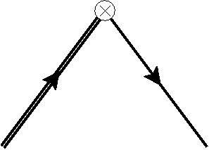
Figure 3: Tadpole correction contribution to the one loop mixing matrix element $\rho_{1}$. The double lines indicate heavy quarks, the single line the light quark and the cross represents the tadpole insertion.

This correction contributes to $\zeta_{11}^{\,(V_{0})}$ and is given by

$$\zeta_{11}^{u_{0}}=u_{0}^{(1)}.$$ (101)

We use the Landau link definition of the tadpole correction coefficient, $u_{0}^{(1)}=0.7503(1)$, when calculating $\rho_{1}$.

In Table 7 we give our results for the matching coefficients for the spatial components of the heavy-light vector current with massless HISQ light quarks and NRQCD heavy quarks.

Table 7: One-loop matching coefficients for the spatial vector current with massless HISQ light quarks. See the caption accompanying Table 6 for more details.

$aM_{0}$	$\rho_{0}^{\,(V_{k})}$	$\zeta_{10}^{\,(V_{k})}$
3.297	-0.046(2)	0.0319(1)
3.263	-0.045(2)	0.0322(1)
3.250	-0.045(2)	0.0323(1)
2.688	-0.034(2)	0.0382(1)
2.660	-0.034(2)	0.0385(1)
2.650	-0.034(2)	0.0386(1)
2.620	-0.033(2)	0.0391(1)
1.910	0.007(2)	0.0513(1)
1.890	0.009(2)	0.0518(1)
1.832	0.020(2)	0.0532(1)
1.826	0.020(2)	0.0532(1)

V.2 Massive Quarks

In Table 8 we tabulate our results for the matching coefficients for $V_{0}$ with massive HISQ light quarks and NRQCD heavy quarks.

Table 8: One-loop matching coefficients for the temporal vector current with massive HISQ quarks. All results use stability parameter $n=4$ in the NRQCD action. For $\eta_{0}^{\,(V_{0})}$ the quoted uncertainties are the errors from each contribution added in quadrature, whilst for $\tau_{10}^{\,(V_{0})}$ the uncertainty is purely the statistical error from numerical integration.

$aM_{0}$	$am_{0}$	$\eta_{0}^{\,(V_{0})}$	$\tau_{10}^{\,(V_{0})}$
3.297	0.8260	-0.151(3)	-0.0488(1)
3.263	0.8180	-0.148(3)	-0.0494(1)
2.688	0.6300	-0.121(3)	-0.0647(1)
2.660	0.6450	-0.117(3)	-0.0648(1)
2.650	0.6235	-0.113(3)	-0.0658(1)
2.650	0.6207	-0.112(3)	-0.0659(1)
2.620	0.6270	-0.116(3)	-0.0663(1)
1.910	0.4340	-0.102(3)	-0.0990(1)
1.832	0.4130	-0.098(3)	-0.1043(1)
1.826	0.4120	-0.098(3)	-0.1046(1)

We give our results for the matching coefficients for $V_{k}$ in Table 9. Finally, in Tables 10 and 11, we present our results for the matching coefficients for $A_{0}$ and $A_{k}$ respectively.

Table 9: One-loop matching for spatial vector current with massive HISQ quarks. See the caption accompanying Table 8 for more details.

$aM_{0}$	$am_{0}$	$\eta_{0}^{\,(V_{k})}$	$\tau_{10}^{\,(V_{k})}$
3.297	0.8260	-0.124(5)	0.0420(1)
3.263	0.8180	-0.118(5)	0.0423(1)
2.688	0.6300	-0.025(5)	0.0484(1)
2.660	0.6450	-0.024(5)	0.0488(1)
2.650	0.6235	-0.015(5)	0.0489(1)
2.650	0.6207	-0.014(5)	0.0489(1)
2.620	0.6270	-0.019(5)	0.0493(1)
1.910	0.4340	-0.049(5)	0.0618(1)
1.832	0.4130	-0.059(5)	0.0636(1)
1.826	0.4120	-0.060(5)	0.0638(1)

Table 10: One-loop matching for the temporal axial-vector current with massive HISQ quarks. See the caption accompanying Table 8 for more details.

$aM_{0}$	$am_{0}$	$\eta_{0}^{\,(A_{0})}$	$\tau_{10}^{\,(A_{0})}$
3.297	0.8260	-0.237(5)	-0.1260(1)
3.263	0.8180	-0.232(5)	-0.1269(1)
2.688	0.6300	-0.188(5)	-0.1452(1)
2.660	0.6450	-0.192(5)	-0.1464(1)
2.650	0.6235	-0.183(5)	-0.1468(1)
2.650	0.6207	-0.182(5)	-0.1467(1)
2.620	0.6270	-0.189(5)	-0.1480(1)
1.910	0.4340	-0.219(5)	-0.1853(1)
1.832	0.4130	-0.222(5)	-0.1908(1)
1.826	0.4120	-0.221(5)	-0.1914(1)

Table 11: One-loop matching for the spatial axial-vector current with massive HISQ quarks. See the caption accompanying Table 8 for more details.

$aM_{0}$	$am_{0}$	$\eta_{0}^{\,(A_{k})}$	$\tau_{10}^{\,(A_{k})}$
3.297	0.8260	-0.260(3)	0.0163(1)
3.263	0.8180	-0.260(3)	0.0165(1)
2.688	0.6300	-0.194(3)	0.0216(1)
2.660	0.6450	-0.191(3)	0.0216(1)
2.650	0.6235	-0.183(3)	0.0219(1)
2.650	0.6207	-0.182(3)	0.0320(1)
2.620	0.6270	-0.185(3)	0.0221(1)
1.910	0.4340	-0.091(3)	0.0330(1)
1.832	0.4130	-0.076(3)	0.0348(1)
1.826	0.4120	-0.076(3)	0.0349(1)

VI Summary

We have calculated the one loop matching coefficients required to match the axial-vector and vector currents on the lattice to full QCD. We used the HISQ action, with both massless and massive quarks, for the light quarks and NRQCD for the heavy quarks. As part of the matching procedure we have presented one loop mass and wavefunction renormalisations for both HISQ and NRQCD quarks. We find that the perturbative coefficients are well behaved and none are unduly large.

The matching coefficients for HISQ-NRQCD currents with massless HISQ quarks are important ingredients in the determination of heavy-light mesonic decay parameters from lattice QCD studies H. Na et al. (2012). Recent studies of the $B_{s}$ meson using the relativistic HISQ action for both $b$ and $s$ quarks have been carried out C. McNeile et al. (2012). Such an approach has the advantage that perturbative matching, which is generally the dominant source of error in the extraction of decay constants, is not required. Currently, however, simulations at the physical $b$ quark mass are prohibitively expensive and an extrapolation up to the $b$ quark mass is still needed. Furthermore, simulations of the $B$ meson are not presently feasible, as the use of light valence quarks and close-to-physical $b$ quark masses requires both large lattices and fine lattice spacings. In light of these considerations, the use of an effective theory for heavy-light systems remains the most efficient method for precise predictions of $f_{B_{s}}/f_{B}$ and $f_{B}$. Such calculations require the perturbative matching calculation reported in this article.

The matching calculations reported in this work are also crucial for the HPQCD collaboration’s nonperturbative studies of the semileptonic decays of $B$ and $B_{s}$ mesons with NRQCD and HISQ quarks. On the one hand, matching coefficients with massless HISQ quarks are required for the determination of the $B\rightarrow\pi\ell\nu$, $B\rightarrow K\ell^{+}\ell^{-}$ and $B_{s}\rightarrow K\ell\nu$ decay parameters C. Bouchard (2012). On the other hand, our results for the matching coefficients with massive HISQ quarks will be needed in future calculations of the $B\rightarrow D\ell\nu$ and $B_{s}\rightarrow D_{s}\ell\nu$ decay parameters.

Appendix A The HISQ tuning parameter

In this appendix, we derive expressions for the tree level and one loop tuning parameters, $\epsilon_{\text{tree}}$ and $\epsilon_{1}$. Throughout this appendix we neglect factors of the lattice spacing, $a$, for convenience.

For an onshell particle with momentum given by $p_{\mu}=(iE,0,0,p_{z})$ one defines the kinetic mass as

$$m_{\text{kin}}=\left(\frac{\partial^{2}E}{\partial p_{z}^{2}}\right)^{-1}_{p_{z}=0}.$$ (102)

At nonzero momentum the tree level pole condition becomes

$$m_{0}^{2}={} \left[\sinh(E)-\frac{1+\epsilon_{\text{tree}}}{6}\left(\sinh(E)\right)^{3}\right]^{2}$$

$$-\left[\sin(p_{z})+\frac{1+\epsilon_{\text{tree}}}{6}\left(\sin(p_{z})\right)^{3}\right]^{2},$$ (103)

which, for notational convenience, we write as

$$m_{0}^{2}=[X(E)]^{2}-[Y(p_{z})]^{2}.$$ (104)

Using the relations

$$Y(p_{z}=0)=0,\quad\frac{\partial E}{\partial p_{z}}\bigg{|}_{p_{z}=0}=0,\quad\frac{\partial Y(p_{z})}{\partial p_{z}}\bigg{|}_{p_{z}=0}=1,$$ (105)

and differentiating twice using

$$\frac{\text{d}}{\text{d}p_{z}}=\frac{\partial}{\partial p_{z}}+\frac{\partial E}{\partial p_{z}}\frac{\partial}{\partial E},$$ (106)

we find

$$\left[\left(-X\frac{\partial X}{\partial E}\right)\left(\frac{\partial^{2}E}{\partial p_{z}^{2}}\right)+\left(\frac{\partial Y}{\partial p_{x}}\right)^{2}\right]_{p_{z}=0}=0,$$ (107)

and thus the tree level kinetic mass is

$$m_{\text{kin}}^{(0)}={} X\frac{\partial X}{\partial E}$$

$$={} \cosh(m_{\text{tree}})\sinh(m_{\text{tree}})(1-\Theta)(1-3\Theta).$$ (108)

Here we have defined $\Theta=(1+\epsilon_{\text{tree}})(\sinh(m_{\text{tree}}))^{2}/6$.

Requiring $m_{\text{kin}}^{(0)}=m_{\text{tree}}$ imposes a condition on the tree level tuning parameter that leads to Equation (III.2).

At one loop, the procedure is much the same. The one loop pole condition is

$$(m_{0}-\alpha_{s}\Sigma^{(\mathbb{I})})^{2}={} \left[\widetilde{X}(E)-\sinh(E)\alpha_{s}\Sigma^{(p\!\!\!/)}_{0}\right]^{2}$$

$$-\left[Y(p_{z})-\sin(p_{z})\alpha_{s}\Sigma^{(p\!\!\!/)}_{z}\right]^{2},$$ (109)

where

$$\widetilde{X}(E)=\sinh(E)\left[1-\frac{1+\epsilon}{6}\left(\sinh(E)\right)^{2}\right].$$ (110)

Differentiating twice using Equation (106) leads, after some algebra, to

$$m_{\text{kin}}={} \widetilde{X}\frac{\partial\widetilde{X}}{\partial E}-\alpha_{s}\bigg{\{}\Sigma^{(p\!\!\!/)}_{0}\left(Z_{Q}^{(0)}\right)^{-1}\sinh(m_{\text{tree}})+2m_{\text{tree}}\Sigma^{(p\!\!\!/)}_{z}-m_{0}\frac{\partial}{\partial E}\left[\sinh(E)\Sigma^{(p\!\!\!/)}_{0}-\Sigma^{(\mathbb{I})}\right]$$

$$-m_{0}m_{\text{tree}}\frac{\partial^{2}}{\partial p_{z}^{2}}\left[\sinh(m_{\text{tree}})\Sigma^{(p\!\!\!/)}_{0}-\Sigma^{(\mathbb{I})}\right]\bigg{\}},$$ (111)

where we have only kept terms up to ${\cal O}(\alpha_{s})$.

For convenience, we write this as

$$m_{\text{kin}}=\widetilde{X}\frac{\partial\widetilde{X}}{\partial E}+\alpha_{s}\sigma.$$ (112)

Using the expansions of Equations (42), (43) and (46), we can evaluate the product, $\widetilde{X}\frac{\partial\widetilde{X}}{\partial E}$, at one loop to obtain

$$\widetilde{X}\frac{\partial\widetilde{X}}{\partial E}=m_{\text{tree}}+u_{1}\epsilon_{1}\alpha_{s}+u_{2}m_{1}\alpha_{s},$$ (113)

where

$$u_{1}={} \frac{1}{6}\cosh(m_{\text{tree}})(\sinh(m_{\text{tree}}))^{3}\Big{(}(1+\epsilon_{\text{tree}})(\sinh(m_{\text{tree}}))^{2}-4\Big{)}$$ (114)

$$u_{2}={} (\sinh(m_{\text{tree}}))^{2}\Big{(}1-\frac{1+\epsilon_{\text{tree}}}{6}(\sinh(m_{\text{tree}}))^{2}\Big{)}\bigg{[}1-\frac{1+\epsilon_{\text{tree}}}{2}\Big{(}2(\cosh(m_{\text{tree}}))^{2}+(\sinh(m_{\text{tree}}))^{2}\Big{)}\bigg{]}$$

$$+(\cosh(m_{\text{tree}}))^{2}\Big{(}1-\frac{1+\epsilon_{\text{tree}}}{2}(\sinh(m_{\text{tree}}))^{2}\Big{)}^{2}$$ (115)

We can therefore write Equations (112) and (113) as

$$m_{\text{kin}}=m_{\text{tree}}+\alpha_{s}\Big{(}\nu^{(\epsilon)}\epsilon_{1}+\nu^{(\Sigma)}\Big{)},$$ (116)

with $\nu^{(\Sigma)}$ and $\nu^{(\epsilon)}$ given by

$$\nu^{(\Sigma)}={} u_{2}m_{1}^{(\Sigma)}+\sigma,$$ (117)

$$\nu^{(\epsilon)}={} u_{1}+u_{2}m_{1}^{(\epsilon)},$$ (118)

and

$$m_{1}^{(\Sigma)}={} \sinh(m_{\text{tree}})\Sigma^{(p\!\!\!/)}_{0}-\Sigma^{(\mathbb{I})},$$ (119)

$$m_{1}^{(\epsilon)}={} \frac{1}{6}Z_{Q}^{(0)}(\sinh(m_{\text{tree}}))^{3}.$$ (120)

We obtain an expression for the one loop tuning parameter by equating the one loop masses: $m_{\text{kin}}^{(1)}=m_{1}^{(1)}$. The result is

$$\epsilon_{1}=\frac{m_{1}^{(\Sigma)}-\nu^{(\Sigma)}}{\nu^{(\epsilon)}-m_{1}^{(\epsilon)}}$$ (121)

where $\nu^{(\Sigma)}$ and $\nu^{(\epsilon)}$ are given in Equations (117) and (118) respectively.

Appendix B Subtraction functions for numerical integration

At intermediate stages of the lattice-to-continuum matching procedure one encounters infrared (IR) divergent integrals and care is required to ensure that VEGAS can handle them accurately. For diagrams involving massless HISQ fermions, it is usually sufficient to introduce a nonzero gluon mass $\lambda$, fit results to appropriate functions of this mass and then extract the IR finite parts. For massive HISQ fermions, on the other hand, it is often necessary to include specific subtraction terms into the integrand in order to stabilize the VEGAS integrations. In this appendix we list examples of such subtraction terms. Given an IR divergent integral,

$${\cal I}=C_{F}\int\!\frac{\mathrm{d}^{4}k}{(2\pi)^{4}}\;\,{\cal F}_{\text{lat}}(k,\lambda),$$ (122)

where $C_{F}=4/3$ is a color factor (the quadratic Casimir operator) required to correctly normalize the infrared divergences. We employ subtraction terms in the following way:

$${\cal I}={} C_{F}\int\!\frac{\mathrm{d}^{4}k}{(2\pi)^{4}}\;\left\{{\cal F}_{\text{lat}}(k,\lambda)-{\cal F}_{\text{sub}}(k,m_{eff},\Lambda,\lambda)\right\}$$

$${}\qquad+F(m_{\text{eff}},\Lambda,\lambda),$$ (123)

where

$$F(m_{\text{eff}},\Lambda,\lambda)=C_{F}\int\!\frac{\mathrm{d}^{4}k}{(2\pi)^{4}}\;{\cal F}_{\text{sub}}(k,m_{\it eff},\Lambda,\lambda).$$ (124)

Here $\Lambda$ is a cutoff imposed on ${\cal F}_{\text{sub}}$ such that ${\cal F}_{\text{sub}}\equiv 0$ for $k^{2}\geq\Lambda^{2}$, and $m_{\text{eff}}$ is defined below. The full expression for ${\cal I}$ in (123) does not, of course, depend on $\Lambda$. We have done the calculations with two different values for $\Lambda$, e.g. $a\Lambda$ = 2 and 3, to check this.

The choice for ${\cal F}_{\text{sub}}$ is far from unique. One wants a function of $k_{\mu}$ with the same IR behaviour as the original integrand ${\cal F}_{\text{lat}}$, that is, however, simple enough that the integral in the “addback” function, $F(m_{\text{eff}},\Lambda,\lambda)$, can be evaluated with relative ease. One natural choice is the integrand of the corresponding continuum theory Feynman diagram ${\cal F}_{\text{cont}}$. This is what has often been done in the literature. For massive fermions there remains the question of what fermion mass to use in ${\cal F}_{\text{cont}}$. It was suggested in Y. Kuramashi (1998) to pick a mass, denoted by $m_{\text{eff}}$, such that ${\cal F}_{\text{sub}}(k,m_{\text{eff}},\Lambda,\lambda)$ mimics as closely as possible the correct $k_{\mu}\rightarrow 0$ limit in the denominator of the lattice fermion propagator. For instance in the continuum theory one would have (we work in Euclidean space), for onshell quarks with external momentum $p_{\mu}\rightarrow(im,\vec{0})$, a fermion propagator with denominator given by

$$\text{denom}=(p-k)^{2}+m^{2}\rightarrow k^{2}-2imk_{0}.$$ (125)

Taking a hint from (125) we pick $m_{\text{eff}}$ by first setting the external momentum to $p_{\mu}=(im_{\text{tree}},\vec{0})$, expanding the denominator of the free HISQ propagator around $k_{0}=0$ and then looking for the coefficient of $(-2ik_{0})$. One finds,

$$m_{\text{eff}}=\cosh(m_{\text{tree}})\sinh(m_{\text{tree}})(1-\Theta)(1-3\Theta),$$ (126)

where $\Theta$ is defined after (108). We recognize this as $m_{\text{kin}}^{(0)}$, given in (108), so that

$$m_{\text{eff}}=m_{\text{kin}}^{(0)}\equiv m_{\text{tree}},$$ (127)

a result that may not come as a surprise. We note, however, that the last equality in (127) holds only because we have tuned $\epsilon_{\text{tree}}$ to ensure $m_{\text{kin}}^{(0)}=m_{\text{tree}}=m^{(0)}_{\text{pole}}$. This was not the case for uses of $m_{\text{eff}}$ in the past Y. Kuramashi (1998); S. Groote and J. Shigemitsu (2000) involving massive Clover fermions.

Following the guidlines described above, the subtraction term for the rainbow diagram correction to the massive HISQ wave function renormalization $Z_{Q}$ becomes

$${\cal F}_{\text{sub}}^{Z_{Q}} = \theta(\Lambda^{2}-k^{2})\left\{\frac{4(k_{0}^{2}+b^{2}/4)\,((k^{2})^{2}-b^{2}k_{0}^{2})}{(k^{2}+\lambda^{2})\,((k^{2})^{2}+b^{2}k_{0}^{2})^{2}}\right.$$ (128)

$$-(\xi-1)\left.\frac{k_{0}^{2}(b^{2}+2k^{2})}{k^{2}(k^{2}+\lambda^{2})\,((k^{2})^{2}+b^{2}k_{0}^{2})}\right\},$$

with $b=2m_{\text{tree}}$. This leads to an addback function

$$F^{Z_{Q}}={} \frac{2}{3\pi}\bigg{\{}\left[\log\left(\frac{\Lambda^{2}}{\lambda^{2}}\right)-\log\left(\frac{W_{1}}{b}\right)-2\frac{\Lambda^{2}}{b^{4}}(b^{2}+3\Lambda^{2})-\frac{\Lambda W_{0}}{b^{4}}(b^{2}-6\Lambda^{2})\right]$$

$$-\frac{(\xi-1)}{2}\left[\log\left(\frac{\Lambda^{2}}{\lambda^{2}}\right)-\log\left(\frac{W_{1}}{b}\right)+2\frac{\Lambda^{2}}{b^{4}}(2b^{2}+\Lambda^{2})-\frac{\Lambda W_{0}}{b^{4}}(3b^{2}+2\Lambda^{2})\right]\bigg{\}},$$ (129)

where $W_{0}\equiv\sqrt{b^{2}+\Lambda^{2}}$ and $W_{1}\equiv[\Lambda+W_{0}]$.

Similarly, for the one-loop vertex correction for a scattering diagram involving $V_{0}$ one has in Feynman gauge,

$${\cal F}_{\text{sub}}^{V_{0}}=\frac{\theta(\Lambda^{2}-k^{2})\left\{k_{0}^{2}\,(k^{2}+b^{2})\;-\;\frac{b}{2M}(\vec{k}^{2})^{2}\right\}}{[(k^{2})^{2}+b^{2}k_{0}^{2}]\,[k_{0}^{2}+(\vec{k}^{2}/(2M))^{2}]\,[k^{2}+\lambda^{2}]}.$$ (130)

And for the annihilation diagram involving $V_{k}$ one has,

$${\cal F}_{\text{sub}}^{V_{k}}=\frac{\theta(\Lambda^{2}-k^{2})\left\{k_{0}^{2}\,(k^{2}+b^{2})\;+\;\frac{b}{2M}(\vec{k}^{2})^{2}\right\}}{[(k^{2})^{2}+b^{2}k_{0}^{2}]\,[k_{0}^{2}+(\vec{k}^{2}/(2M))^{2}]\,[k^{2}+\lambda^{2}]}.$$ (131)

The only difference between (130) and (131) is the relative sign between the two terms in the numerator, i.e. the sign of the term linear in $m_{\text{tree}}$. This is as it should be, since for annihilation one has an incoming anti-HISQ quark with the on-shell condition $p_{\mu}\rightarrow(-im_{\text{tree}},\vec{0})$ replacing the outgoing HISQ quark of the scattering process. The two terms in the numerator each lead to linear IR divergent results which cancel in the case of $V_{0}$ leaving just a logarithmic IR divergence. For $V_{k}$ one ends up with an expression with both linear and logarithmic IR divergent terms as is required. We have not attempted to integrate ${\cal F}_{\text{sub}}^{V_{0}}$ or ${\cal F}_{\text{sub}}^{V_{k}}$ in closed form to obtain analytic expressions for the addback functions $F^{V_{0}}$ and $F^{V_{k}}$. Instead we reduced the integrals to 1D integrals in the radial variable $0\leq k\leq\Lambda$ and used VEGAS again to evaluate them.

References

- E. Lunghi and A. Soni (2011a) E. Lunghi and A. Soni, Phys. Lett. B 697, 323 (2011a), arXiv:1010.6069.
- E. Lunghi and A. Soni (2011b) E. Lunghi and A. Soni, arXiv:1104.2117 [hep-ph] (2011b).
- J. Laiho et al. (2010) J. Laiho, E. Lunghi, and R.S. Van de Water, PoS FPCP 040 (2010).
- J. Laiho et al. (2012) J. Laiho, E. Lunghi, and R.S. Van de Water, (2012), arXiv:1204.0791.
- C. McNeile et al. (2012) C. McNeile et al., Phys. Rev. D 85, 031503 (2012), arXiv:1110.4510.
- H. Na et al. (2012) H. Na et al., Phys. Rev. D 86, 034506 (2012), arXiv:1202.4914.
- C. Bouchard (2012) C. Bouchard et al., (2012), arXiv:1209.0104.
- P. Weisz (1983) P. Weisz, Nucl. Phys. B 212, 1 (1983).
- P. Weisz and R. Wohlert (1984) P. Weisz and R. Wohlert, Nucl. Phys. B 236, 397 (1984).
- G. Curci et al. (1983) G. Curci, P. Menotti, and G. Paffuti, Phys. Lett. B 130, 205 (1983).
- M. Luescher and P. Weisz (1985) M. Luescher and P. Weisz, Commun. Math. Phys. 97, 59 (1985).
- G.P. Lepage and P.B. Mackenzie (1993) G.P. Lepage and P.B. Mackenzie, Phys. Rev. D 48, 2250 (1993).
- E. Follana et al. (2007) E. Follana et al., Phys. Rev. D 75, 054502 (2007), arXiv:hep-lat/0610092.
- E. Follana et al. (2008) E. Follana et al., Phys. Rev. Lett. 100, 062002 (2008), arXiv:0706.1726.
- C. McNeile et al. (2010) C. McNeile et al., Phys. Rev. D 82, 034512 (2010), arXiv:1004.4285.
- E.B. Gregory et al. (2011) E.B. Gregory et al., Phys. Rev. D 83, 014506 (2011), arXiv:1010.3848.
- R.J. Dowdall et al. (2012a) R.J. Dowdall et al., (2012a), arXiv:1207.5149.
- G.P. Lepage (1999) G.P. Lepage, Phys. Rev. D 59, 074502 (1999).
- M. Wingate et al. (2003) M. Wingate et al., Phys. Rev. D 67, 054505 (2003).
- A. Gray et al. (2005) A. Gray et al., Phys. Rev. D 72, 094507 (2005), arXiv:hep-lat/0507013.
- R.J. Dowdall et al. (2012b) R.J. Dowdall et al., Phys. Rev. D 85, 054509 (2012b), arXiv:1110.6887.
- E. Gulez et al. (2004) E. Gulez, J. Shigemitsu, and M. Wingate, Phys. Rev. D 69, 074501 (2004), arXiv:hep-lat/0312017.
- S. Groote and J. Shigemitsu (2000) S. Groote and J. Shigemitsu, Phys. Rev. D 62, 014508 (2000), arXiv:hep-lat/0001021.
- B.P.G. Mertens et al. (1998) B.P.G. Mertens, A.S. Kronfeld, and A.X. El-Khadra, Phys. Rev. D 58, 034505 (1998), arXiv:hep-lat/9712024.
- A.G. Hart et al. (2004) A.G. Hart, R.R. Horgan, and L.C. Storoni, Phys. Rev. D 70, 034501 (2004), arXiv:hep-lat/0402033.
- A.G. Hart et al. (2009) A.G. Hart et al., Comp. Phys. Commun. 180, 2698 (2009), arXiv:0904.0375.
- I.T. Drummond et al. (2002) I.T. Drummond et al., Phys. Rev. D 66, 094509 (2002), arXiv:hep-lat/0208010.
- I.T. Drummond et al. (2003a) I.T. Drummond et al., Nucl. Phys. B (Proc. Suppl.) 119, 470 (2003a).
- I.T. Drummond et al. (2003b) I.T. Drummond, A. Hart, R.R. Horgan, and L.C. Storoni, Phys. Rev. D 68, 057501 (2003b), arXiv:hep-lat/0307010.
- A.G. Hart et al. (2007) A.G. Hart, G.M. von Hippel, and R.R. Horgan, Phys. Rev. D 75, 014008 (2007), arXiv:hep-lat/0609002.
- E.H. Mueller et al. (2011) E.H. Mueller, A.G. Hart, and R.R. Horgan, Phys. Rev. D 83, 034501 (2011), arXiv:1011.1215.
- T.C. Hammant et al. (2011) T.C. Hammant et al., Phys. Rev. Lett. 107, 112002 (2011), arXiv:1105.5309.
- G.P. Lepage (1980) G.P. Lepage, CLNS-80/447 (1980).
- G.M. von Hippel (2010) G.M. von Hippel, Comput. Phys. Commun. 181, 705 (2010), arXiv:0910.5111.
- Y. Kuramashi (1998) Y. Kuramashi, Phys. Rev. D 58, 034507 (1998), arXiv:hep-lat/9705036.
- C.J. Morningstar (1993) C.J. Morningstar, Phys. Rev. D 48, 2265 (1993).
- (37) A.G. Hart et al., In preparation.
- C.J. Morningstar and J. Shigemitsu (1998) C.J. Morningstar and J. Shigemitsu, Phys. Rev. D 57, 6741 (1998), arXiv:hep-lat/9712016.
- C.J. Morningstar and J. Shigemitsu (1999) C.J. Morningstar and J. Shigemitsu, Phys. Rev. D 59, 094504 (1999), arXiv:hep-lat/9810047.
- E. Braaten and S. Fleming (1995) E. Braaten and S. Fleming, Phys Rev D 52, 181 (1995).
- B.D. Jones and R.M. Woloshyn (1999) B.D. Jones and R.M. Woloshyn, Phys. Rev. D 60, 014502 (1999), arXiv:hep-lat/9812008.
- P. Boyle and C.T.H. Davies (2000) P. Boyle and C.T.H. Davies, Phys. Rev. D 62, 074507 (2000), arXiv:hep-lat/0003026.
- R.R. Horgan et al. (2009) R.R. Horgan et al., Phys. Rev. D 80, 074505 (2009).
- S. Collins et al. (2001) S. Collins et al., Phys. Rev. D 63, 034505 (2001).