On the Bauschinger effect in supercoooled melts under shear: results from mode coupling theory and molecular dynamics simulations

Abstract

We study the nonlinear rheology of a glass-forming binary mixture under the reversal of shear flow using molecular dynamics simulations and a schematic model of the mode-coupling theory of the glass transition (MCT). Memory effects lead to a history-dependent response, as exemplified by the vanishing of a stress-overshoot phenomenon in the stress–strain curves of the sheared liquid, and a change in the apparent elastic coefficients around states with zero stress. We investigate the various retarded contributions to the stress response at a given time schematically within MCT. The connection of this macroscopic response to single-particle motion is demonstrated using molecular-dynamics simulation.

I Introduction

Dense liquids exhibit slow relaxation processes in thermal equilibrium, characterized by a time scale $\tau$ that diverges as the liquid is driven to structural arrest into an amorphous solid Kob (2003). This opens a window rich in nonlinear phenomena under flow, both amenable to experiment and theoretical treatment. It is of interest, because the externally imposed flow strongly disturbs the equilibrium relaxation processes. More precisely, given a typical single-particle relaxation time scale $\tau_{0}$, we consider shear flow with deformation rate $\dot{\gamma}$ such that $\text{{Pe}}_{0}=\dot{\gamma}\tau_{0}\ll 1$, but $\text{{Pe}}=\dot{\gamma}\tau\gg 1$. This nonlinear rheology has in particular been studied in colloidal dispersions and soft-matter systems, where the mesoscopic size of the constituent particles implies relaxation times of $\mathcal{O}(\text{s})$, easily probed by moderate flow in experiment. In the flowing steady state, shear thinning is the most prominent phenomenon: Larson (1999); Oswald (2009) the apparent viscosity of the sheared fluid decreases rapidly with increasing shear rate $\dot{\gamma}$. Quite generally, the flowing steady state is characterized by a nonlinear relation between the macroscopic stress $\sigma$ and the applied shear rate $\dot{\gamma}$.

Going beyond the steady state, the behavior under start-up flow has received particular attention. As a steady shear flow of rate $\dot{\gamma}$ is suddenly switched on at $t=0$, stresses $\sigma$ increase from zero (assuming the experiment was started in an equilibrated and hence stress-free configuration) to their steady-state value $\sigma(\dot{\gamma})$. The resulting stress-strain curve $\sigma(\gamma)$, measured as a function of applied deformation $\gamma=\dot{\gamma}t$ for $t>0$, exhibits a peculiar intermediate maximum, termed stress overshoot. This is typically found in amorphous metals Schuh, Hufnagel, and Ramamy (2007), or (for different reasons) polymer melts Dealy and Larson (2006). The maximum of the $\sigma(\gamma)$ curve has been linked to material stability: it can be taken as a yield stress that separates reversible (linear and nonlinear) elastic deformation at small strains from irreversible plastic flow induced by larger deformations. More recently, stress overshoots have also been discussed in soft colloidal systems, underlining a generic mechanism applicable in a wide variety of system classes Zausch et al. (2008); Koumakis et al. (2012); Siebenbürger, Ballauff, and Voigtmann (2012); Amann et al. (2012).

As a transient phenomenon, the stress overshoot is susceptible to the history of sample preparation. Molecular dynamics simulations have addressed this focusing on the shear-molten amorphous solid, where a systematic dependence was found on the waiting time $t_{\rm age}$ between sample preparation and flow start-up Varnik, Bocquet, and Barrat (2004), as long as the start-up configuration is not fully equilibrated, $t_{\rm age}\ll\tau$.

In the engineering literature it is well established that the stress-strain curve depends on the deformation history of the sample. One particular example was found empirically by Johann Bauschinger in the 1880’s during experiments on various steels Bauschinger (1886): these materials typically are softer under compressional load after having been subject to tension. This is, in the strict sense, called the Bauschinger effect. As an abstraction, take the case where pre-shear is applied in one particular direction, and consider the modified stress–strain curve measured if shear is then applied in the opposite direction. Typically, the regime of elastic deformation shrinks, so that plastic rearrangements dominate much earlier than in an initially unstrained sample.

Reversing the shear rate, which we will call ’Bauschinger effect’ also, in the following, has been discussed Langer (2008) in the framework of the shear-transformation-zone theory (STZ), where one attributes internal degrees of freedom to the STZs, which carry the memory of the deformation history. Recent simulation studies of the Bauschinger effect Karmakar, Lerner, and Procaccia (2010) in a system quenched into its low-temperature glassy state have been analyzed in terms of anisotropic elastic constants that arise due to the deformation history.

It is a matter of current debate whether and how the rheological properties of amorphous materials deep in the glassy state (here referred to as essentially the $T\to 0$ case), and at much higher temperaturs in the melt, are related. In athermal systems, concepts like STZs Langer (2008) and avalanches of yielding events Chattoraj, Caroli, and Lemaître (2010) are widely recognized as useful to rationalize macroscopic behavior. But the range of applicability of these approaches is not well understood when dealing with liquids close to their glass transition, where thermal fluctuations dominate yielding mechanisms that may be qualitatively different from, say, athermal jamming Voigtmann (2011). The rheology of dense liquids is the realm of a recent extension of the mode-coupling theory of the glass transition (MCT) to sheared colloidal systems Fuchs and Cates (2002a, 2009); Brader, Cates, and Fuchs (2012). Intriguingly, some of the macroscopic phenomena are quite alike in both quasi-athermal systems and liquids driven by thermal noise.

Here we investigate, both by mode-coupling theory and computer simulation, the nonlinear rheology under flow reversal in the initially equilibrated liquid state, without referring to $T\to 0$ properties. The initial stress overshoot is shown to vanish if the flow is reversed in the steady state. Hence, the Bauschinger effect does not require an explanation associated with properties of the quenched glass or aging phenomena. We study its connection to the time-dependent memory of past flow that is typical for dense liquids, by investigating the effect of flow reversal applied at various times during the initial evolution from equilibrium to steady state. A clear separation between reversible elastic rearrangements and irreversible plastic flow emerges. We connect the macroscopic stress response to microscopic particle motion, quantified through the transient mean-squared displacements.

The paper is organized as follows: Section II contains the exposition of the theoretical approach, and section III gives an overview of the simulation. In Sec. IV we discuss the comparison between theory and simulation, and the insights thereby gained. Section V concludes with an outlook.

II Theory

Our theoretical approach is based on the mode-coupling theory of the glass transition (MCT) Götze (2009), as extended to deal with nonlinear rheology in the integration-through transients (ITT) formalism Fuchs and Cates (2002a); Brader, Cates, and Fuchs (2012). ITT-MCT is a microscopic (albeit approximate) theory describing the dynamical correlation functions of the wave-vector dependent density fluctuations in glass-forming liquids. Suitably generalized Green-Kubo relations provide the nonequilibrium transport coefficients in the nonlinear-response regime; within MCT, they are expressed as integrals over the density correlators. The coupling coefficients of the theory are fully determined by knowing the equilibrium static structure of the liquid. The theory then predicts an ideal glass transition to occur as a bifurcation transition: smooth changes in control parameters such as density or temperature bring about a discontinuous change in the long-time behavior of the density correlation functions. These decay to zero in the equilibrium liquid, but attain a finite long-time limit, the glass form factor, in the ideal glass. The theory compares semi-quantitatively to the linear rheology measured in colloidal hard sphere dispersions Crassous et al. (2008); Siebenbürger et al. (2009); Siebenbürger, Fuchs, and Ballauff (2012).

Since the full microscopic theory is rather cumbersome to solve, various simplifications have been devised. Schematic models try to capture mathematically the essence of the bifurcation transition by reducing the number of correlation functions to a few or only one, at the cost of neglecting spatial information. The important correlations contained in the schematic models are temporal ones. Memory effects are contained in generalized friction kernels depending on (up to) three times. Causality is automatically enforced, and the flow history of the sample is contained in the friction-kernels via time- or strain-dependent elastic coefficients and structural relaxation functions. The latter describe plastic deformation, and their nonlinear equations of motion are the heart of the theory. The non-Markovian equations of the schematic models contain a small number of fitting parameters that mimic the relation between the equilibrium structure (encoding the interaction potential) and the theory’s coupling coefficients. Smooth and regular variations of the parameters lead to dramatic elasto-plastic and viscoelastic changes in the structural relaxation and non-linear rheology. The interpretation of the effects in terms of spatially dependent particle rearrangements can not be achieved by the schematic model, and thus it remains unresolved to which degree ’force-chains’, ’heterogeneities’, or specific ’plastic rearrangement centers’ are described in a (presumably) space-averaged manner.

II.1 Schematic MCT Model

A schematic MCT model for the time-dependent rheology of colloidal suspensions was introduced in Ref. [Brader et al., 2009]; it has been used to study large-amplitude oscillatory shear Brader et al. (2010), mixed flows Farage and Brader (2012), and double-step strain Voigtmann et al. (2012), and generalizes a model used to analyze stationary flow curves Crassous et al. (2008); Siebenbürger et al. (2009). In the model, the nonlinear generalization of the Green-Kubo relation for the shear-stress tensor element $\sigma\equiv\sigma_{xy}$ reads, imposing spatially homogeneous but otherwise arbitrary simple shear flow with rate $\dot{\gamma}$ in the $x$-direction, with gradient in the $y$-direction,

$$\sigma(t)=\int\limits_{-\infty}^{t}\!\text{d}t^{\prime}\dot{\gamma}(t^{\prime})G(t,t^{\prime},[\dot{\gamma}])\,.$$ (1)

The generalized shear modulus $G(t,t^{\prime},[\dot{\gamma}])$ depends on the full flow history encoded in the time-dependent shear rate $\dot{\gamma}(t)$. Outside the steady state, it also depends on the two times corresponding to the underlying fluctuations separately. In the spirit of MCT, we approximate the shear modulus in terms of the transient density correlation function $\Phi(t,t^{\prime})$,

$$G(t,t^{\prime})=v_{\sigma}(t,t^{\prime})\,\Phi^{2}(t,t^{\prime}).$$ (2)

Here, an elastic coefficient $v_{\sigma}$ appears that was set to a constant in the original formulation of the model Brader et al. (2009). It measures the strength of stress fluctuations caused by pair-density fluctuations. The microscopic theory implies a relation between $\Phi(t,t^{\prime})$ and $G(t,t^{\prime})$ that involves an integration over wave vectors, including nontrivial weights that depend on time since density fluctuations are advected by shear. It is therefore plausible to extend the original schematic model by allowing for a prefactor $v_{\sigma}(t,t^{\prime})$ that depends on time through the accumulated strain $\gamma(t,t^{\prime})=\int_{t^{\prime}}^{t}\dot{\gamma}(s)\,\text{d}s$,

$$v_{\sigma}(t,t^{\prime})=v_{\sigma}^{*}\,\cdot\left(1-\left(\frac{\gamma\left(t,t^{\prime}\right)}{\gamma^{*}}\right)^{2}\right)\,\exp\left(-\left(\frac{\gamma\left(t,t^{\prime}\right)}{\gamma^{**}}\right)^{2}\right).$$ (3)

Symmetry dictates that the direction of the strain does not matter, leading to an even function $v_{\sigma}=v_{\sigma}(\gamma(t,t^{\prime})^{2})$. Equation (3) generalizes the time-dependent coupling first introduced for constant shear rates in Ref. [Amann et al., 2012], where it was justified by a comparison with fully microscopic ITT-MCT calculations in two dimensions. The functional form is chosen simple enough for rapid numerical implementation and allows for a quantitative discussion of stress overshoots in model colloidal suspensions Amann et al. (2012); Laurati et al. (2012). The parameter $v_{\sigma}^{*}$ sets the scale of the generalized shear modulus. We obtain it by matching it to the linear-response low-frequency plateau modulus $G_{\infty}$ of the simulation. The shear elastic constant $G_{\infty}$ itself often is called ‘shear modulus’, and can, e.g., be measured in the low-frequency linear elastic modulus of the glass, $G^{\prime}(\omega\to 0)=G_{\infty}$, or as one of the two Lamé-coefficients of an isotropic solid Klix et al. (2012). At a critical strain scale $\gamma^{\ast}$, the time-dependent modulus becomes negative and the stress-strain curve exhibits an overshoot with its peak at the critical strain. $\gamma^{\ast\ast}$ describes the decay of the overshoot. To reduce the number of free parameters, we keep it linearly proportional Amann et al. (2012) to $\gamma^{*}$.

The time-dependent elastic coefficient given in Eq. (3) is carefully chosen to become negative in a small strain window relevant for the decay of the correlation functions. Doing so, it allows to circumvent an obvious limitation of the schematic model: setting $v_{\sigma}=\text{const.}$, Eq. (2) has a definite sign. In startup shear, cf. Eq. (1), this implies that $\sigma(t)$ varies monotonically with accumulated strain. The original schematic model hence does not describe stress overshoot phenomena. Motivated by the full microscopic expression of ITT-MCT Fuchs and Cates (2009); Amann et al. (2012) and the observation that the wave-vector dependent MCT, even with further isotropy assumptions, produces a stress overshoot through a small negative dip in $G(t,t^{\prime})$, cf. Ref. [Zausch et al., 2008], Eq. (3) is a simple way to incorporate the phenomenology. In the following, we take it as one established way to match the startup stress–strain curves (see below for a comparison to simulation), and discuss the consequences of the history-integral formulation of Eq. (1) under flow reversal.

The schematic density correlator is the solution of a Mori-Zwanzig-like memory equation

$$\dot{\Phi}(t,t^{\prime})+\Gamma\left(\Phi(t,t^{\prime})+\int\limits_{t^{\prime}}^{t}\!\text{d}t^{\prime\prime}\,m(t,t^{\prime\prime},t^{\prime})\dot{\Phi}(t^{\prime\prime},t^{\prime})\right)=0,$$ (4)

with initial condition $\Phi(t,t^{\prime})=1-\Gamma(t-t^{\prime})+\ldots$. Here $\Gamma$ denotes the initial decay rate of the density correlator, which corresponds to a reciprocal microscopic relaxation time. We take $\Gamma$ to be independent of the shear rate.

To close this equation of motion, MCT approximates the memory kernel $m$ through a nonlinear polynomial of the correlation functions. In contrast to a Markovian approximation, this postulates that the kernel relaxes on the same time scale as the correlator, and that both need to be obtained self-consistently. Conceptually, this is motivated by the assumption that stress fluctuations captured in $m$ arise from slow structural rearrangements, which themselves are captured in $\Phi$. The simplest schematic model that recovers the asymptotic behavior found for typical quiescent glass-forming liquids is the F₁₂ model Götze (2009), whose extension to time-dependent shear reads

$$m(t,t^{\prime\prime},t^{\prime})=h(t,t^{\prime\prime})\,\left[v_{1}\Phi(t,t^{\prime\prime})+v_{2}\Phi^{2}(t,t^{\prime\prime})\right].$$ (5)

The parameters $v_{1}$ and $v_{2}$ are the coupling coefficients driving the system through the glass transition. There is a line of bifurcation points $(v_{1}^{c},v_{2}^{c})$, and we pick $v_{2}=v_{2}^{c}$ and $v_{1}=v_{1}^{c}+\epsilon/(\sqrt{2}-1)$ with $v_{1}^{c}=2(\sqrt{2}-1)$ as in previous work. The parameter $\epsilon$ controls the distance to the glass transition: $\epsilon<0$ corresponds to liquid states, where the correlation function decays to zero in the quiescent system, on a time scale $\tau$ that diverges as $\epsilon\to 0$. States with $\epsilon>0$ are idealized glass states, where the quiescent correlation function attains a positive long-time limit, $\lim_{t\to\infty,t\gg t^{\prime}}\Phi(t,t^{\prime})=f>0$. This value is called the non-ergodicity parameter or glass form factor. The elastic constant in the model then follows as $G_{\infty}=v_{\sigma}^{*}f^{2}$.

One of the predictions of ITT-MCT is that (steady) shear melts the glass; the correlation functions even in the glass show shear-induced decay due to a loss of memory Fuchs and Cates (2002a, b). In the schematic model, this is modeled by an ad-hoc strain-reduction function,

$$h(t,t^{\prime})=\frac{1}{1+\left(\gamma(t,t^{\prime})/\gamma_{c}\right)^{2}}.$$ (6)

Symmetry again dictates that $h$ is an even function of the accumulated strain. The parameter $\gamma_{c}$ is a critical strain and describes how fast the memory of the glass decays due to its deformation. In principle, the microscopic form of the MCT equation suggests further combinations of the three times to appear in Eq. (5), as exploited for example in Refs. [Brader et al., 2009] and [Voigtmann et al., 2012]. We neglect these terms here, to make contact with earlier schematic-model analyses of the nonlinear steady-state rheology of colloidal suspensions Crassous et al. (2008); Siebenbürger et al. (2009); Siebenbürger, Fuchs, and Ballauff (2012). In principle, the strain-reduction function $h$ could also contain negative regions, as arises in the stress-density coupling $v_{\sigma}$. This could cause the transient correlator $\Phi$ to become negative for intermediate times as seen in computer simulations and microscopic ITT-MCT calculations in two dimensions Krüger, Weysser, and Fuchs (2011). For simplicity, this is neglected.

II.2 Bauschinger effect

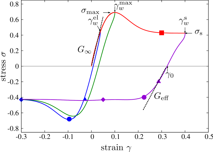
Figure 1: Linear plot of the stress-strain relation $\sigma(\gamma)$ at fixed density and shear rate for various flow histories: startup flow with constant shear rate (red), flow reversal in the steady state (s, purple), from the elastic regime (el, blue), and from the point of the stress overshoot (max, green). The linear increase with the quiescent elastic modulus $G_{\infty}$ in startup, and with $G_{\text{eff}}$ after shear-reversal are indicated by dotted lines. Characteristic stress–strain points, whose transient modulus is discussed in the text, are marked by symbols: The red square gives the stationary stress. It corresponds to an integration along the line from A to B in Fig. 7. Triangles mark stresses after flow reversal in the linear regime and correspond to an integration along the line C’ to E’. Discs mark stresses after flow reversal in the overshoot regime and are obtained via integrations along the line C to E in Fig. 7.

The flow history we consider in this work is given by two intervals of constant shear rate:

$$\dot{\gamma}(t)=\begin{cases}0&\text{for $t<0$,}\\ +\dot{\gamma}&\text{for $0<t<t_{w}$,}\\ -\dot{\gamma}&\text{for $t>t_{w}$.}\end{cases}$$ (7)

We mainly discuss a fixed value for $\dot{\gamma}$, and different waiting times $t_{w}$ over which the “pre-shear” in the positive direction is applied. These times correspond to an accumulated strain $\gamma_{w}=\dot{\gamma}t_{w}$. The amount of this pre-strain is decisive and determines the stress–strain curve after switching. Figure 1 presents typical results obtained in the schematic model as unmodified stress-versus-strain curves; it serves to introduce the flow history and characteristic parameters. After startup of shear at $t=0$, the system first undergoes an elastic transient, characterized by a stress–strain curve $\sigma(\gamma)$ that is approximately linear, $\sigma\approx G_{\infty}\gamma$, given by the quiescent elastic shear modulus. At the end of this regime, the $\sigma$-versus-$\gamma$ curves becomes sublinear, until the position of the overshoot is reached at some strain $\gamma^{\text{max}}$, typically of the order of $10\%$. At large strains, one reaches the steady state characterized by a constant $\sigma(\gamma\to\infty)=\sigma_{s}$ independent of $\gamma$. For the flow reversal, we consider switching the shear rate at three typical points in either regime: $\gamma_{w}^{\text{el}}$ inside the elastic transient, $\gamma_{w}^{\text{max}}$, and $\gamma_{w}^{\text{s}}$ in the steady state. The $\gamma_{w}$ values are marked in Fig. 1. A value $\gamma_{w}^{\text{s}}=0.4$ in the schematic model turns out to be sufficient so that no further $\gamma_{w}$ dependence is observed for larger values besides a trivial shift. To ease the interpretation of the curves at different switching times, we choose $\gamma_{w}^{\text{el}}$ such that the corresponding stress is equal to the steady-state one, $\sigma(\gamma_{w}^{\text{el}})=\sigma(\gamma_{w}^{\text{s}})$. Generally, after reversing the flow direction, the stress first decreases back to zero, defining a strain value $\gamma_{0}$. The stress–strain curves in later figures will be compared in a $|\sigma|$-versus-$|\gamma-\gamma_{0}|$ representation. While it does hide the “hysteresis” loop which can be recognized in Fig. 1, and which is familiar in the engineering literature, it simplifies the quantitative analysis.

All calculations in the schematic model are done with parameters that have been found typical in applications of predecessors of the model to large amplitude oscillatory shear Brader et al. (2010), and especially to startup flow Amann et al. (2012); Laurati et al. (2012). The values are: $\Gamma=100$, $\gamma_{c}=0.75$, $\gamma^{\ast}=0.1$, and $\gamma^{\ast\ast}=0.133$; see also Fig. 2. The considered state in Fig. 1, which will be analyzed in more detail in Figs. 8 and 9, is a glass very close to the glass transition in order to achieve a large separation of the structural dynamics from the short-time one; $\epsilon=10^{-4}$. The shear rate $\dot{\gamma}=5\times 10^{-3}$, for which the Bauschinger effect is studied, corresponds to a rather small Peclet number, which in the model is given by Pe${}_{0}=\dot{\gamma}/\Gamma$, and thus takes the value $5\times 10^{-5}$. These two values provide access to the asymptotic regime of ITT-MCT for $\epsilon\to 0$ and Pe${}_{0}\ll 1$. Slightly different $\epsilon$ and $\dot{\gamma}$ values are used in the comparisons to the simulations in Sec. IV.

Figure 1 contains a wealth of information, which will be discussed in Sec. IV together with the simulation results.

III Simulation

We perform nonequilibrium molecular dynamics computer simulation for a glass-forming binary mixture. Particles interact through a purely repulsive soft-sphere potential. Denoting particle species by $\alpha,\beta$, the truncated Lennard-Jones potential due to Weeks, Chandler, and Andersen Weeks (1971) reads

$$V_{\alpha\beta}^{\text{WCA}}(r)=\begin{cases}4\epsilon_{\alpha\beta}\left[\left(\frac{\sigma_{\alpha\beta}}{r}\right)^{12}-\left(\frac{\sigma_{\alpha\beta}}{r}\right)^{6}+\frac{1}{4}\right]&\text{$r<r_{c,\alpha\beta}$}\\ 0&\text{else}\end{cases}\,,$$

where $r_{c,\alpha\beta}=2^{1/6}\sigma_{\alpha\beta}$ is a cutoff for the interaction range. To ensure continuity of force and conservation of total energy in the NVE ensemble, we apply a smoothing function, $V_{\alpha\beta}(r)=V_{\alpha\beta}^{\text{WCA}}(r)S_{\alpha\beta}(r)$ with $S_{\alpha\beta}(r)=(r-r_{c,\alpha\beta})^{4}/[h^{4}+(r-r_{c,\alpha\beta})^{4}]$ with $h=10^{-2}\sigma_{\alpha\beta}$ Zausch et al. (2010). We choose units of energy such that $\epsilon_{\alpha\beta}=1$, and units of length such that $\sigma_{\text{AA}}=1$. The unit of time is given by $\sqrt{m_{\text{A}}\sigma^{2}_{\text{AA}}/\epsilon_{\text{AA}}}$ where $m_{\text{A}}=m_{\text{B}}=1$ are the masses of the particles. For the smaller particles, $\sigma_{\text{BB}}=5/6$, and the mixture is additive, $\sigma_{\text{AB}}=(\sigma_{\text{AA}}+\sigma_{\text{BB}})/2$. This system, albeit with differing masses, has been previously studied in the quiescent state and identified as a model glass former in its equimolar composition Hedges et al. (2007).

The system is coupled to a dissipative particle dynamics (DPD) thermostat: the equations of motion read Groot and Warren (1997)

$$m_{\alpha}\dot{\vec{r}}_{\alpha} =\vec{p}_{\alpha}\,,$$ (8a)

$$\dot{\vec{p}}_{\alpha} =\vec{F}_{\alpha}^{\text{C}}(\{\vec{r}\})+\vec{F}_{\alpha}^{\text{D}}(\{\vec{r},\vec{p}\})+\vec{F}_{\alpha}^{\text{R}}(\{\vec{r}\})\,.$$ (8b)

where $\vec{r}$ and $\vec{p}$ are positions and momenta of the particles, and $\vec{F}^{i}$ denotes conservative ($i=\text{C}$), dissipative ($i=\text{D}$), and random ($i=\text{R}$) forces. With the interparticle separation $r_{ij}=|\vec{r}_{i}-\vec{r}_{j}|$ between particles $i$ and $j$ of species $\alpha$ and $\beta$,

$$\vec{F}_{\alpha}^{\text{C}} =-\sum_{j\neq i}\vec{\nabla}V_{\alpha\beta}(r_{ij})$$ (9)

$$\vec{F}_{\alpha}^{\text{D}} =-\sum_{j\neq i}\zeta w^{2}(r_{ij})(\hat{\vec{r}}_{ij}\cdot\vec{v}_{ij})\hat{\vec{r}}_{ij}$$ (10)

$$\vec{F}_{\alpha}^{\text{R}} =\sum_{j\neq i}\sqrt{2k_{\text{B}}T\zeta}\,w(r_{ij})\mathcal{N}_{ij}\hat{\vec{r}}_{ij}$$ (11)

Here, $\vec{v}_{ij}=\vec{p}_{i}/m_{i}-\vec{p}_{j}/m_{j}$ is the relative velocity between the two particles, and $\hat{\vec{r}}_{ij}=(\vec{r}_{i}-\vec{r}_{j})/r_{ij}$ their unit separation. The appearance of the relative velocity in the dissipative force is crucial to obtain local momentum conservation and Galilean invariance Zausch et al. (2010). $w(r)$ is a cutoff function, set to $w=1$ for $r<r_{c,\text{DPD}}/2$ and $w=0$ elsewhere. We have chosen $r_{c,\text{DPD}}=1.7r_{c,\alpha\alpha}$ in our simulations. $\zeta$ is a parameter controlling the strength of friction forces; we set $\zeta=10$. This parameter is not crucial for the results to be discussed Zausch et al. (2008). The $\mathcal{N}$ are Gaussian normal random variables.

The DPD equations of motion, Eq. (8), are integrated with a generalized velocity Verlet algorithm Peters (2004). This algorithm integrates the reversible Hamiltonian part of the equations with the velocity Verlet scheme and then partially re-equilibrates the two-particle momenta, ensuring a Boltzmann distribution in equilibrium. A time step of $\delta t=5\times 10^{-4}$ (in the specified units of time) is employed. Two different neighbor lists are implemented, one for the force calculations, and one for the DPD thermostat. The simulation consists of $N=2N_{\text{A}}=1300$ particles in a three-dimensional box with volume $V=L^{3}$ and linear dimension $L=10\sigma_{\text{AA}}$, corresponding to a number density $\rho=1.3$. At this density, no signs of crystallization or phase separation were observed in the studied temperature range from $T=5$ to $T=0.4$. A glass transition point is estimated as $T_{c}\approx 0.347$ according to mode-coupling theory. In the following we focus on the equilibrated fluid at $T=0.4$. Initial equilibration proceeded by using $\delta t=10^{-3}$, assigning new velocities every 50 integration time steps. Equilibration was checked by the decay of the incoherent intermediate scattering function at a wave number corresponding to a typical interparticle separation $q=2\pi/\sigma_{\text{AA}}$: runs were long enough to observe the decay of the correlation function to zero at long times. A set of $200$ independently equilibrated configurations served as initial configurations for the production runs employing the DPD thermostat.

Shear is applied in the $x$-direction with a gradient in $y$-direction and a positive shear rate $\dot{\gamma}$ initially. Planar Couette flow is imposed by periodic Lees-Edwards boundary conditions Lees and Edwards (1972): the periodic image of a particle leaving or entering the simulation box in $y$-direction is displaced in $x$-direction according to the strain $\pm\dot{\gamma}L$.

The macroscopic response of the system to imposed shear flow is measured through the stress tensor. In the specified coordinate system, the dominant contribution at low shear rates is its $xy$-component, given by the Kirkwood formula Binder and Kob (2005),

$$\sigma_{xy}=\langle\hat{\sigma}_{xy}\rangle=-\frac{1}{V}\left\langle\sum_{i=1}^{N}\left[m_{i}v_{i,x}v_{i,y}+\sum_{j\neq i}r_{ij,x}F_{ij,y}\right]\right\rangle\,.$$ (12)

The first term is a kinematic contribution, while the second is the virial contribution incorporating the nonhydrodynamic forces exerted on each particle. Angular brackets indicate canonical averages. In the following, we restrict the discussion of the Bauschinger effect to one, rather high, exemplary shear rate, $\dot{\gamma}=5\times 10^{-3}$.

IV Results and discussion

IV.1 Comparison of simulation and theory

We begin by a discussion of the properties of the computer-simulated system under startup of flow and in its steady state. Qualitatively, they reproduce earlier results Zausch et al. (2008). Here, they serve to determine the schematic model parameters prior to investigation of the Bauschinger effect.

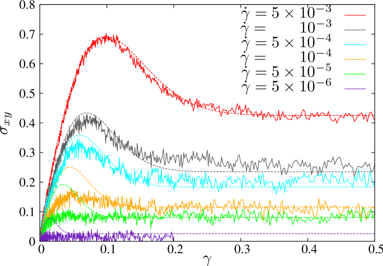
Figure 2: Plot of the stress-strain curves $\sigma(\gamma)$ at fixed temperature for various shear rates. The dashed lines show the MCT results for $\Gamma=100$, $\epsilon=-10^{-4}$, $\gamma_{c}=0.75$, $v_{\sigma}^{*}=97$, and $\gamma_{\ast\ast}/\gamma_{\ast}=1.33$. $\gamma_{\ast}$ is $10^{-1},7\times 10^{-2},6\times 10^{-2},4.5\times 10^{-2},3.5\times 10^{-2},1.5\times 10^{-2}$ for decreasing shear rates $\dot{\gamma}$.

Figure 2 shows the stress–strain curves $\sigma(\gamma)$ obtained after switch-on of steady shear at $t=0$, for various shear rates $\dot{\gamma}$ at one particular temperature in the supercooled liquid. For small $\dot{\gamma}$, the system behaves as a linear viscoelastic fluid, and the stress quickly reaches its steady state value, rising monotonically from zero. As the shear rate is increased, an intermediate overshoot in the $\sigma$-versus-$\gamma$ curve appears. Depending on $\dot{\gamma}$, the typical strain reached at the position of the overshoot is a few percent; at the highest shear rates this value is about $10\%$. It is in agreement with earlier observations Zausch et al. (2008), and one can argue that this typical strain corresponds to a typical size of nearest-neighbor cages that are being broken by shear Petekidis, Moussaïd, and Pusey (2002).

From the large-$\gamma$ limit of the stress–strain curves, one obtains the steady-state flow curve, $\sigma_{\text{s}}(\dot{\gamma})$. The values extracted from our simulation and the schematic-model fits exhibit shear-thinning: The stress increases sublinearly with the rate. Note in Fig. 2 that the values of $\sigma$ are given in simulation units, where $kT=0.4$. This confirms that the stresses we observe are dominated by thermal motion, since $\sigma_{\text{s}}=O(kT/\sigma_{\alpha\alpha}^{3})$. This compares well to recent investigations of colloidal suspensions Siebenbürger et al. (2009); Siebenbürger, Ballauff, and Voigtmann (2012); Amann et al. (2012); Laurati et al. (2012). The precise numerical value is found to differ among different systems, as it somewhat depends on the interaction potential and mixture parameters in experimental samples.

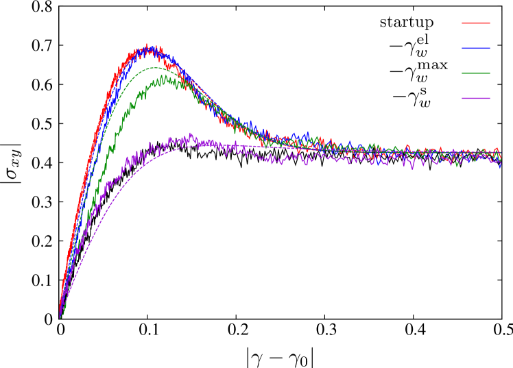
Figure 3: Linear plot of the stress-strain relation $|\sigma(|\gamma-\gamma_{0}|)|$ at fixed temperature and shear rate for various flow histories: starting from equilibrium (EQ, red line), after flow reversal in the steady state (S, purple), from the elastic regime (el, blue), and from the point of the stress overshoot (max, green). Reversal at $\gamma_{w}^{\text{s}}=0.4$ is in the steady state as seen from comparing with reversal at $\gamma_{w}^{\text{s}}=75$ (black data). Smooth lines result from the schematic model.

The solid lines in Fig. 2 are fits with the schematic MCT model including the time-dependent vertex for the Green-Kubo relation. These fits were optimized to reproduce the shape of the overshoot at the largest shear rate (for which the Bauschinger effect will be discussed below). Further adjustments to improve agreement at the lower shear rates may well be possible, but note that the form of the overshoot is dictated by the empirical choice of $v_{\sigma}(t,t^{\prime})$.

The parameters of the schematic MCT model can be determined by fitting the simulation data in startup shear. Using a fit procedure similar to the one outlined in Ref. [Amann et al., 2012] we arrive at the values listed in the caption of Fig. 2. The parameters $\Gamma$ and $\epsilon$ determine the short- and long-time relaxation scales $\tau_{0}$ and $\tau$ in the model. They are fixed by a comparison of the quiescent equilibrium correlation functions at a typical intermediate wave number corresponding to the first peak of the static structure factor. Linear-response fluctuations also allow to determine $v_{\sigma}^{*}$, corresponding to the plateau modulus $G_{\infty}$ and hence setting the units of stresses in the model. The parameters $\gamma_{c}$, $\gamma^{*}$, and $\gamma^{**}$ are then tuned to the startup rheology data, taking the shear rate $\dot{\gamma}$ nominally from the simulation.

Once the parameters given in the caption of Fig. 2 have been fixed, the predictions of the schematic model regarding the modification of the stress–strain curve under flow reversal are parameter-free.

We now turn to the discussion of the Bauschinger effect. Figure 3 shows the main result of the computer simulation, viz. the stress–strain curves in the $|\sigma|$-versus-$|\gamma-\gamma_{0}|$ representation, i.e., shifted and inverted such that they all start from a stress-free state and display the behavior as a function of the additional strain imposed on this configuration. Curves for various $\gamma_{w}$ are shown, as discussed above. They all agree at large strains by construction, confirming that the steady-state stress does not depend on the shear history. Comparing first the startup curve, $\gamma_{w}=0$, with the one for reversal in the steady-state, $\gamma_{w}=\gamma_{w}^{\text{s}}$, the Bauschinger effect becomes most apparent. The two curves differ in two main aspects: the linear slope at small deformations is lower, and the overshoot is gone in the curve corresponding to oppositely straining the (steadily) pre-sheared configuration. This holds for shear-reversal throughout the stationary state, as shown by the two curves for $\gamma_{w}^{\text{s}}=0.4$ and $\gamma_{w}^{\text{s}}=75$ included in Fig. 3. Both these differences arise because the system undergoes plastic deformations during pre-shear: confining the pre-shear to small strains, $\gamma_{w}=\gamma_{w}^{\text{el}}$, so that flow reversal takes place inside the initial elastic-deformation regime, the overshoot is maintained almost unchanged, as is the effective elastic coefficient extracted from the initial rise of the stress–strain curve. The cross-over between elasticity-dominated and plasticity-dominated pre-strain occurs gradually, as the curve for $\gamma_{w}=\gamma_{w}^{\text{max}}$ exemplifies.

The solid lines in Fig. 3 represent the schematic-MCT model calculations. The line corresponding to $\gamma_{w}=0$ is a result of the fitting procedure described above. All the other theory curves then follow from the structure of the ITT-MCT equations. They describe the computer-simulation data extremely well, and capture both the decrease of the overshoot and the decrease of the effective elastic coefficient.

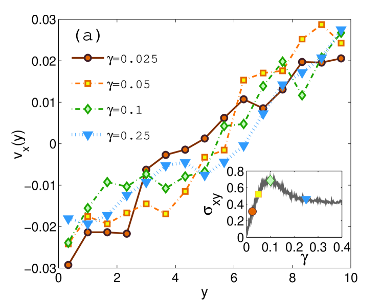
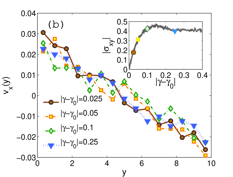
Figure 4: Velocity profiles $v_{x}(y)$ as a function of position along the gradient direction $y$ for various times after application of a new flow direction. (a) Starting from a quiescent configuration (EQ), shear in $+x$ direction. (b) Starting from the resulting steady state (S) at $\gamma^{s}_{w}=0.4$, shear in $-x$ direction. Insets mark the points for which profiles are shown along the stress-strain curves. A total $100$ independent configurations are averaged within a small time window to obtain the depicted graphics.

Before continuing the discussion, it is worth pointing out that none of the features we discuss appear to be explained by, or connected to shear banding or other inhomogeneous flow effects. To demonstrate this, we show in Fig. 4 the velocity profiles obtained from the simulation at various instants in time, both under forward shear and the subsequently reversed shear. To improve statistics, the instantaneous velocities were averaged over all the configurations and over a small time window of width $\Delta t=0.1$. Insets in the figure mark the points for which the velocity profiles $v_{x}(y)$ are shown; they all follow the linear behavior $v_{x}(y)=\dot{\gamma}y$ expected from homogeneous simple shear, to within statistical noise. Similar results have also been obtained under startup shear Zausch et al. (2008). It appears that the small time needed to establish a linear velocity profile under Lees-Edwards boundary conditions is not relevant for our discussion. In Fig. 4 only the case for flow reversal in the steady state is shown, but qualitatively the same result is found for the velocity profiles obtained after switching the shear direction at the smaller $\gamma_{w}^{\text{max}}$ or $\gamma_{w}^{\text{el}}$. Stress overshoot phenomena have been linked to shear banding Moorcroft, Cates, and Fielding (2011), but it appears that this mechanism is not relevant for our system. Indeed, our results are compatible with a recent study suggesting a density-dependent critical Péclet number for the appearance of shear bands Besseling et al. (2010).

IV.2 Interpretation in a generalized Maxwell model

To understand the history dependence of the stress–strain curves, let us split the integral in Eq. (1) into two parts. For $t>t_{w}$, write

$$\sigma(t)=\sigma_{\text{I}}(t)-\sigma_{\text{II}}(t)$$ (13)

with the summands

$$\sigma_{\text{I}}(t) =\dot{\gamma}\int_{0}^{t_{w}}\text{d}t^{\prime}\,G(t,t^{\prime})\,,$$ (14a)

$$\sigma_{\text{II}}(t) =\dot{\gamma}\int_{t_{w}}^{t}\text{d}t^{\prime}\,G(t,t^{\prime})=\dot{\gamma}\int_{t_{w}}^{t}\text{d}t^{\prime}\,G(t-t^{\prime})\,.$$ (14b)

In the last term, $\sigma_{\text{II}}(t)$, the condition $t_{w}<t^{\prime}<t$ is fulfilled, so that the correlation and strain functions entering the integral are dependent on one-time only and describe the transient between an equilibrium and a stationary state. Hence, this contribution is trivially related to the startup curve, $-\sigma_{\text{II}}(t+t_{w})=\sigma_{\text{start}}(t)$; see below in Sect. IV.3 for details.

To simplify the discussion, let us consider an ad-hoc generalization of the Maxwell model of viscoelastic liquids to shear-thinning fluids. Keeping the form of the Green-Kubo equation, we approximate the generalized shear modulus, Eq. (2), by

$$G(t,t^{\prime})\approx G_{M}(t,t^{\prime})=v_{\sigma}(t,t^{\prime})e^{-(t-t^{\prime})|\dot{\gamma}(t^{\prime})|/\tilde{\gamma}_{c}}\,.$$ (15)

For the case of constant shear and constant $v_{\sigma}$, this form shows the same qualitative features as the shear-molten glass in schematic MCT Fuchs and Cates (2002b). To generalize this nonlinear Maxwell model to unsteady flows is neither trivial nor unique, but assuming the rate of decorrelation to be set by the instantaneous shear rate, the above ansatz appears plausible, if somewhat crude Siebenbürger, Ballauff, and Voigtmann (2012). In the present case it even simplifies further because $|\dot{\gamma}(t^{\prime})|=\dot{\gamma}$. The integrals determining $\sigma(t)$ and its two contributions $\sigma_{\text{I}}$ and $\sigma_{\text{II}}$ can then be solved analytically when inserting the form of $v_{\sigma}(t,t^{\prime})$ given above. In order to quantitatively match the startup stress–strain curve of the generalized Maxwell model with the schematic model, we set $\tilde{\gamma}_{c}=\gamma_{c}/3$.

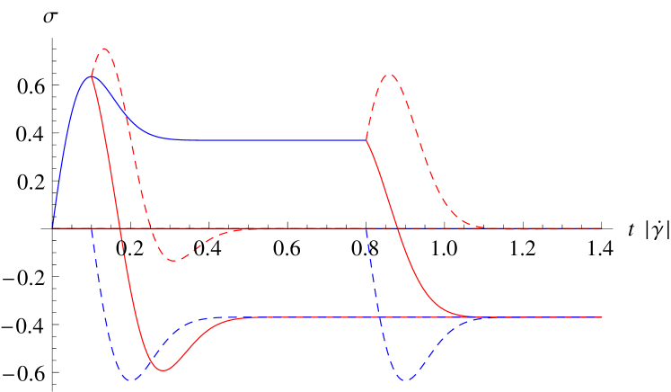
Figure 5: Bauschinger effect as illustrated by a generalized Maxwell model (see text). Solid lines are $\sigma(t)$ as a function of normalized time, $|\dot{\gamma}|t$, for the case $\gamma_{w}=0.1$ corresponding to $\gamma_{w}^{\text{max}}$ and $\gamma_{w}=0.8$ corresponding to $\gamma_{w}^{\text{s}}$. Dashed lines display the contributions $\sigma_{\text{I}}(t)$ (upper, red) and $\sigma_{\text{II}}(t)$ (lower, blue).

The response for large $t_{w}$ can now be understood, recalling that the integral appearing in $\sigma_{\text{I}}(t)$ is dominated by $t^{\prime}\approx t_{w}$, where the integrand is still non-vanishing. The accumulated strain entering the correlation functions can then be written as $\gamma_{tt^{\prime}}=\dot{\gamma}(2t_{w}-(t+t^{\prime}))\approx\dot{\gamma}(t-t_{w})$. Hence, $\sigma_{\text{I}}$ becomes a function of $t-t_{w}$ only, and the precise time of switching the flow becomes irrelevant (as it takes place in the steady state after startup). This is confirmed by numerical evaluation and also in the simulation, by varying $\gamma_{w}^{\text{s}}$. At $t=t_{w}$, $\sigma_{\text{I}}$ is nothing but the value of the startup curve; as $t\to\infty$, this contribution vanishes since the functions in the integrand will generally decay. Furthermore, at $t\approx t_{w}+\gamma_{c}/\dot{\gamma}$, a maximum occurs as the relevant strain $|\gamma_{tt^{\prime}}|\approx\gamma_{c}$ when the integral is dominated by large $t^{\prime}$. This maximum cancels out the corresponding minimum from $\sigma_{\text{II}}$, so that the stress overshoot is generically expected to vanish. This is shown in Fig. 5 for the case $\gamma_{w}=0.8$. For $t_{w}\approx\gamma_{w}^{\text{max}}/\dot{\gamma}$, however, the integral determining $\sigma_{\text{I}}$ will have two relevant contributions, namely $t^{\prime}\approx t_{w}$ as well as $t^{\prime}\approx 0$, since the relevant strain at both these times equals $\gamma_{c}$. Hence, $\sigma_{\text{I}}(t)$ in this case displays first a maximum and then a minimum, as exemplified in Fig. 5 for the case $\gamma_{w}=0.1$. The minimum is responsible for $\sigma_{\text{I}}(t)$ not to cancel the stress overshoot contained in $\sigma_{\text{II}}(t)$. Obviously, as $t_{w}\to 0$, the contribution $\sigma_{\text{I}}(t)$ vanishes, so that perfect elastic recovery is obtained in this limit. While the generalized Maxwell model simplifies the interpretation, the next sections show that broadly equivalent curves follow from the present schematic model, which provides a fundamental basis for this simplification. It exhibits a two step process, where the final decay recovers the properties of Eq. (15).

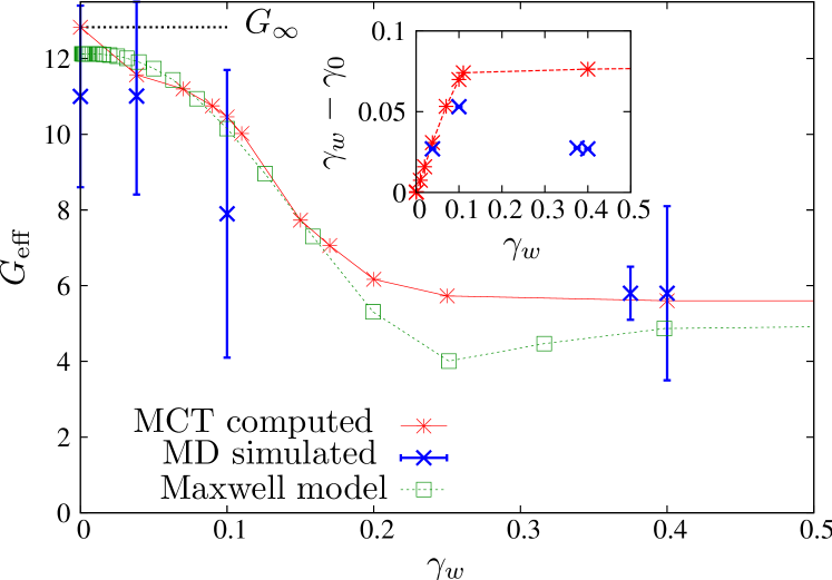
Figure 6: Linear stress responses $G_{\text{eff}}=d\sigma/d\gamma|_{|\gamma-\gamma_{0}|=0.025}$ from simulation, fits of the schematic model, and Maxwell model as labeled for various waiting strains $\gamma_{w}$. The inset gives the strain $\gamma_{w}-\gamma_{0}$ required for the stress to reduce to zero after shear reversal. To include the simulation point for $\gamma_{w}^{s}=75$, this value has been divided by 200, using that the precise value of $\gamma_{w}$ is irrelevant in the steady state.

We now turn to a discussion of the effective shear moduli, obtained as $G_{\text{eff}}=d\sigma/d\gamma|_{|\gamma-\gamma_{0}|=0.025}$. They measure the effective elasticity remaining until the shear-driven relaxation sets in. Figure 6 displays the results from the schematic MCT model (red and blue stars) together with the values extracted from the simulation data (blue crosses). The agreement is quite satisfactory, noting that only the initial value at $\gamma_{w}=0$ is a result of a fitting procedure. One observes a marked decrease of $G_{\text{eff}}$ around $\gamma_{w}\approx 0.1$, the position of the overshoot in the startup curve. Hence, pre-shear indeed softens the material, but only by plastic deformation. Also shown in Fig. 6 are the results from the generalized Maxwell model; qualitatively the same trend is seen. In the Maxwell model, we could not find a closed expression to determine $\gamma_{0}$; but the effective shear modulus defined as $\gamma\to\gamma_{w}$ for $t\to t_{w}+0$ can be evaluated analytically. It again follows the trend seen in the figure, albeit with an even lower limiting value at large $\gamma_{w}$.

A missing information on the simulated stress-strain curve remains $\gamma_{0}$, the strain value where the stress-free state is achieved after strain reversal. Its qualitative behavior can be understood easily. Assuming that $G_{\text{eff}}$ is unchanged for small $\gamma_{w}$, the relations $\sigma(t_{w})=G_{\text{eff}}\gamma_{w}$ and $0=\sigma(t_{0})=\sigma(t_{w})-G_{\text{eff}}(\gamma_{0}-\gamma_{w})$ hold. As a result, $\gamma_{0}=2\gamma_{w}$. Linearity holds even if $G_{\text{eff}}$ changes, but the prefactor is somewhat different, as observed in the simulations. For large $\gamma_{w}$, $0=\sigma(t_{0})=\sigma_{\text{ss}}-G_{\text{eff}}(\gamma_{0}-\gamma_{w})$, and the constant value in Fig. 6 is indeed roughly $\sigma_{\text{ss}}/G_{\text{eff}}\approx 0.4/6\approx 0.07$.

IV.3 Discussion of the history dependence in the schematic model

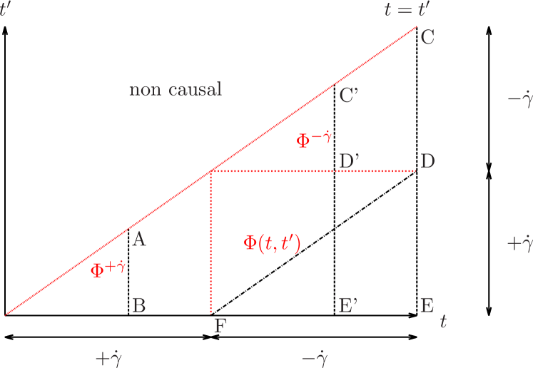
Figure 7: View on the $t-t^{\prime}$-plane, with the three different time regimes for the density correlator $\Phi$. As the $h$-function depends only on the absolute value of $\dot{\gamma}$, the one-time-solutions $\Phi^{(+\dot{\gamma})}$ and $\Phi^{(-\dot{\gamma})}$ are equal.

To understand the history dependence of the stress–strain curves within the schematic ITT-MCT model requires to analyze the time-dependence of the correlator which encodes plastic deformations, and to combine it with the one of the elastic coefficient $v_{\sigma}$, which encodes strain-dependent anelasticity. The structure of Eq. (4) and the time-dependence of the accumulated strain suggests to split the integration domain into three regimes, as shown in Fig. 7. It sketches the corresponding integration paths in the $t-t^{\prime}$–plane leading to the stresses shown in Fig. 1 using Eq (2). Immediately, the strain follows from Eq. (7) (remembering that $t^{\prime}<t$):

$$\gamma(t,t^{\prime})=\begin{cases}\dot{\gamma}\left(t-t^{\prime}\right)&\text{for $0<t^{\prime}<t<t_{w}$,}\\ \dot{\gamma}\left(2t_{w}-(t+t^{\prime})\right)&\text{for $0<t^{\prime}<t_{w}<t$,}\\ -\dot{\gamma}\left(t-t^{\prime}\right)&\text{for $t_{w}<t^{\prime}$,}\end{cases}$$ (16)

which identifies the three regimes. An integration for $t^{\prime},t<t_{w}$ gives the startup stress–strain curve, the integration for $t^{\prime}<t_{w}<t$ gives the stress contribution $\sigma_{I}$ in Eq. (14a), and the integration for $t_{w}<t^{\prime},t$ the contribution $\sigma_{II}$ in Eq. (14b). Recall that the correlators appearing in the MCT model are transient correlation functions, i.e., they are formed with the equilibrium distribution function always, although the full nonequilibrium dynamics appears in their propagator. A correlation function $\Phi(t,t^{\prime})$ hence contains only information on the flow history in the interval $[t^{\prime},t]$. In particular, the correlation functions defined for $0<t^{\prime}<t<t_{w}$ are given by the startup transient solution $\Phi^{(\dot{\gamma})}$ for $\dot{\gamma}(t)=+\dot{\gamma}$ of the model; the same holds true for those defined for $t_{w}<t^{\prime}<t$, since there the shear rate is constant and the direction of shear cannot enter by symmetry. Because the strain in these two time regimes depends on the time difference only (see Eq. (16)), the correlator $\Phi^{(\dot{\gamma})}(t-t^{\prime})$ also depends on the time difference only. This greatly reduces the complexity of Eq. (4) and allows the use of well-established integration schemes to solve

$$\dot{\Phi}^{(\dot{\gamma})}(s)+\Gamma\Phi^{(\dot{\gamma})}(s)+\Gamma\int\limits_{0}^{s}\!\text{d}s^{\prime}\,m^{(\dot{\gamma})}(s-s^{\prime})\dot{\Phi}^{(\dot{\gamma})}(s^{\prime})=0,$$

$$m^{(\dot{\gamma})}(s)=h(\gamma(s))\left[v_{1}\Phi^{(\dot{\gamma})}(s)+v_{2}\Phi^{(\dot{\gamma})}(s)^{2}\right]\;.$$ (17)

Here, $s=t-t^{\prime}$ abbreviates the time difference. The correlation function for $t^{\prime}<t_{w}<t$ however remains fully two-time dependent, as here the strain depends on $t+t^{\prime}$. It is convenient to split the integral appearing in Eq. (4) explicitly at $t^{\prime\prime}=t_{w}$,

$$\partial_{t}\Phi(t,t^{\prime})+\Gamma\Phi(t,t^{\prime})+\Gamma\int\limits_{t^{\prime}}^{t_{w}}\!\text{d}t^{\prime\prime}\,m(t,t^{\prime\prime},t^{\prime})\dot{\Phi}^{(\dot{\gamma})}(t^{\prime\prime}-t^{\prime})$$

$$+\Gamma\int\limits_{t_{w}}^{t}\!\text{d}t^{\prime\prime}\,m^{(\dot{\gamma})}(t-t^{\prime\prime})\partial_{t^{\prime\prime}}\Phi(t^{\prime\prime},t_{w})=0\;,$$ (18)

Here, $m^{(\dot{\gamma})}$ is the same memory kernel also appearing in Eq. (17). Hence, in this formulation, one-time correlators or memory kernels previously calculated enter most succinctly. Supplied with suitable initial conditions, Eq. (18) is a convenient way to deal with instantaneous shear-rate switches numerically Voigtmann et al. (2012).

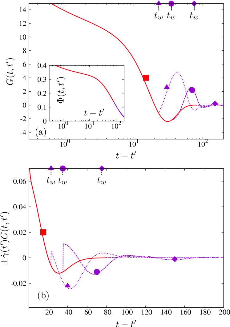
Figure 8: (a) Shear moduli $G(t,t^{\prime})$ after shear reversal at $\gamma^{s}_{w}$ in the steady state, shown for three different fixed times $t$ (respectively strains $\gamma$), as functions of $t-t^{\prime}$. Curves marked with violet triangle, disc, and diamond symbols correspond to points marked with the same symbol in Fig. 1. For times $t-t^{\prime}<t_{w}$, all curves collapse by construction onto the startup result $G(t,0)$ shown in red (marked with a square). The inset shows the corresponding correlators $\Phi(t,t^{\prime})$ (they overlap on the resolution of the figure). (b) Corresponding stress integrands $\pm\dot{\gamma}(t^{\prime})G(t,t^{\prime})$ on a linear $t-t^{\prime}$ axis. Curves after shear reversal which would be negative for $t-t^{\prime}\to 0$ are mirrored to positive initial decay, where they overlap with the startup curve.

Evaluation of a stress $\sigma(\gamma=\int_{0}^{t}dt^{\prime}\dot{\gamma}(t^{\prime}))$ requires integrations of the transient shear modulus along lines at constant $t$ in the plane shown in Fig. 7. The startup curve is obtained along lines of the type from A to B before the shear reversal, where all functions depend on $t-t^{\prime}$. Figures 8 and 9 include the transient density correlators, the transient shear moduli and the integrands of Eq. (1) for this case. As discussed in detail in Refs. [Zausch, 2009, Amann et al., 2012, Laurati et al., 2012], the linear regime in the stress–strain curve is connected to the plateau on intermediate times in $\Phi(t)$ and $G(t)$, and the stress-overshoot to the negative dip in $G(t)$ at late times. Reversing the direction of the shear at a late time when the stationary state was reached at $\gamma^{s}_{w}$, correlators and shear moduli change as shown in Fig. 8. Three different final states are chosen along the reversing stress-strain curve: One in the elastic regime, one in the regime where the stress-maximum is now missing, and one in the late steady regime, where the steady state is reached again. Obviously, the last curves agree with the startup curves (except for the trivial minus sign in the integrand), as the same transient into a steady state is probed. Here the integration path from C to D, where the shear rate takes one definite (negative) value, dominates and the time region, where the shear rate was different, affects the very final transients, only. Moving the final time $t$ to correspond to a strain $\gamma$ of around 10%, where the maximum in the startup curve appears, the transient shear modulus is affected in the negative region. There the strong variation in $v_{\sigma}(t,t^{\prime})$ of Eq. (3) around $\gamma^{*}$ becomes important. Along the integration path from D’ to E’, the memory of the $+\dot{\gamma}$ shear enters, which causes the sign change in $G(t,t^{\prime})$; see the curve marked with a circle in panel (a) of Fig. 8. The integrand of the generalized Green-Kubo relation Eq. (1) varies around zero, see panel (b) of Fig. 8, in the region where the stress overshoot arose. This leads to a cancellation in the integral, and an absence of the maximum in the stress. Shifting the final time $t$ to earlier values in the region, where the startup stress varies linearly with strain, causes the sign change in $G(t,t^{\prime})$ to move to earlier times $t^{\prime}$ as well; see the curve marked with a triangle in panel (a) of Fig. 8. A stronger memory of the shear rate with opposite sign remains. As this arises especially during the final relaxation, the region in $G(t,t^{\prime})$ where stresses are anticorrelated, the overall integral over the transient shear modulus is smaller. As $t$, respectively $\gamma$, lies in the region, where the linear increase in the stress occurs, this explains the softening of the effective elastic constant $G_{\text{eff}}$; see the linear slope indicated in Fig. 1 at the violet triangle. Importantly, in the ITT-MCT approach it arises not by a weakening of the plateau in the transient correlation functions, rather from the aftereffect of the previously stored stresses accumulated during the flow with opposite (positive) shear rate. It thus originates from the final relaxation and does not hold in the proper limit of infinitesimal strain. We chose $\gamma=\gamma^{*}/4$ to measure $G_{\rm eff}$.

Figure 9: Like Fig. 8, but now for shear reversal at $\gamma^{\text{el}}_{w}$ in the elastic regime. The curves end at a time $t-t^{\prime}=\gamma^{\text{el}}_{w}/\dot{\gamma}$, where the memory has not decayed to zero yet. This is as expected, because the system still responds elastic like before the early reversal at $\gamma^{\text{el}}_{w}$; see the blue curve in Fig. 1.

The equivalent discussion holds for reversing the flow during the elastic regime of the startup stress-strain curve. This is indicated by a blue curve in Fig. 1, and the corresponding transient functions are shown in Fig. 9. Again a triangle, circle, and diamond marks final states on the reversing stress–strain curve in the elastic, overshoot, and steady regime. The integration paths in the $t,t^{\prime}$-plane of Fig. 7 do not change qualitatively, but the time $t_{w}$ of switching is now so short that the startup correlators along the line A to B have not decayed to zero. The system responds elastically, and the correlator $\Phi^{(\dot{\gamma})}$ and the modulus $G^{(\dot{\gamma})}$ are still of the order of the plateau value, $f$ respectively $G_{\infty}$. The latter value determines the linear increase of the startup stress-strain curve. The complete discussion of the changes in $G(t,t^{\prime})$ done in respect to Fig. 8 carries over to Fig. 9 with the sole difference that the two-time region D to E (and D’ to E’) dominates at first. By continuity, it reproduces the stress $\sigma(\gamma^{\text{el}}_{w})$, where the flow reversal took place. Because the strain increases with $t+t^{\prime}$ in this region according to Eq. (16), this contribution decays rapidly along the reversing stress-strain curve. It may be neglected beyond $\gamma_{-}\gamma_{w}$, where the initial elastic stress is destroyed. The remaining contribution along the lines C to D or C’ to D’ is equivalent to the startup flow along A to B, and thus after shear rate reversal in the elastic regime, the stress-strain curve agrees closely with the initial startup curve.

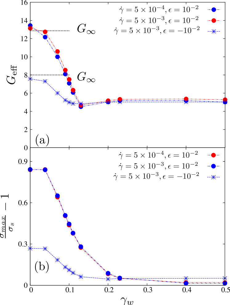
Figure 10: In panel (a), linear stress response $G_{\text{eff}}=d\sigma/d\gamma|_{|\gamma-\gamma_{0}|=0.025}$ as function of waiting strain $\gamma_{w}$ in a fluid and a glass state; for the latter, two different shear rates are shown. The quiescent elastic shear constant $G_{\infty}$ is observed in startup flow.
In panel (b), the corresponding curves are given for the relative stress overshoots $\sigma_{max}/\sigma_{s}-1$.

The preceding discussion of the Bauschinger effect at two typical waiting or reversal times $t_{w}$ corresponding to strains in the elastic and steady regime enables one to rationalize the stress-strain curves for all pre-shears $\gamma_{w}$. Figure 10 summarizes the main findings for two different temperatures close to the glass transition in terms of the effective shear constant $G_{\text{eff}}$ and the relative amplitude of the stress-overshoot $\sigma_{max}/\sigma_{s}-1$. Both change from their quiescent values as soon as $\gamma_{w}$ becomes of the order of $\gamma^{*}$, where the transient shear modulus captures anticorrelated stress fluctuations. The variation of $G_{\text{eff}}$ saturates when $\gamma_{w}>\gamma^{**}$, because then stress correlations have become negligible; then also the overshoot $\sigma_{max}/\sigma_{s}-1$ is gone. Increasing the static correlations in the system, mimicked by $\epsilon$ in the schematic model, increases the elasticity. Because bare Peclet number Pe${}_{0}\ll 1$ are considered, no qualitative difference holds for a liquid and a glassy state. Decreasing the shear rate in the glass, the discussed effects remain and just become somewhat smaller. In a fluid state, the linear response regime would be approached as soon as the dressed Peclet or Weissenberg number Pe$=\dot{\gamma}\tau$ becomes of order unity. This situation where no overshoot arises Amann et al. (2012) and thus flow reversal only mildly affects the stress-strain curve is not shown here.

IV.4 Simulation results on average particle motion

To relate the macroscopic response discussed so far to the microscopic dynamics, we turn to a discussion of simulation results for the density correlation functions under shear. Figure 11 shows as exemplary cases the self-intermediate scattering functions (tagged-particle density-correlation functions) $F^{s}(q,t,t^{\prime})$ in the quiescent equilibrium ($t^{\prime}\to-\infty$, dashed), under startup flow ($t^{\prime}=0$, dash-dotted), and after flow reversal from the steady state ($t^{\prime}=\gamma_{w}^{\text{s}}/\dot{\gamma}$ using $\gamma_{w}^{s}=0.4$, solid lines). Each curve has been sampled by averaging over 200 initial configurations, and we checked that stationarity is achieved comparing with reversal at $\gamma_{w}^{s}=75$. To avoid a discussion of shear-advection effects, wave vectors were chosen with zero component in the shear direction. The equilibrium curves exemplify the typical two-step relaxation found in glass-forming liquids: after an initial fast relaxation to an intermediate plateau, the final decay to zero is characterized by a large time scale $\tau\approx 10^{3}$. This final decay is much more stretched than exponential relaxation. The plateau value depends on the wave number $q$, and for the correlation functions characterizing tagged-particle motion generically decreases with increasing $q$. Steady shear accelerates the dynamics, and induces relaxation from the plateau on a time scale set by $1/\dot{\gamma}$ (with a $q$-dependent prefactor). This relaxation is much closer to exponential, and, for the transient correlation function shown here, even slightly compressed. These qualitative features confirm earlier observations Zausch et al. (2008); Besseling et al. (2007); Krüger, Weysser, and Fuchs (2011). By symmetry, the same is true for the correlation functions probing the reversed-flow regime (solid lines in the figure). However, as in the macroscopic response, a pronounced history dependence is seen: the intermediate plateau is much less pronounced, and the final shear-induced decay shows much more pronounced stretching, in particular at large $q$.

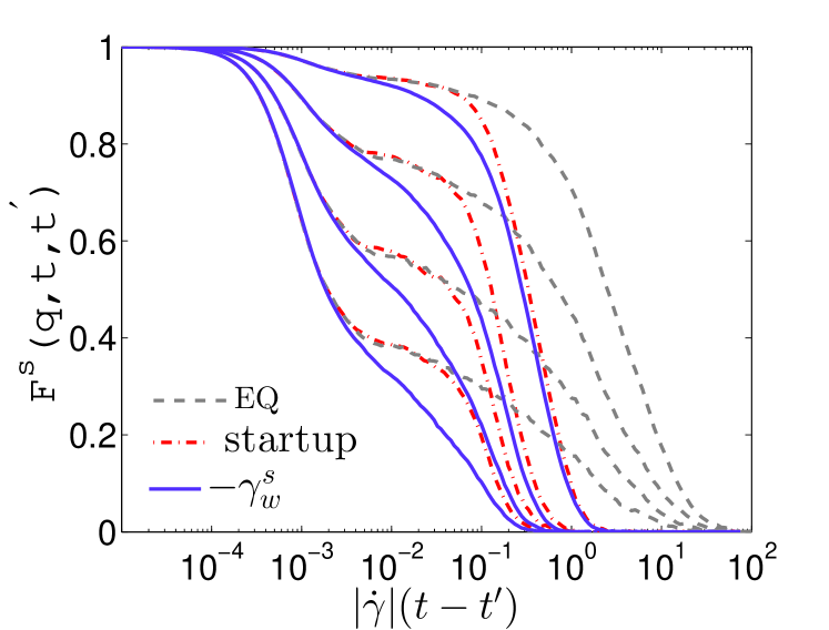
Figure 11: Simulation results of the self intermediate scattering functions $F_{s}(q,t)$ for the B-species in the two directions perpendicular to shear during startup and after shear reversal in the stationary state, for wave vectors $q=[\pi/\sigma_{AA},{2\pi}/\sigma_{AA},{3\pi}/\sigma_{AA},{4\pi}/\sigma_{AA}]$ in descending order. A total 200 independent simulational runs are averaged to obtain these graphics. The corresponding equilibrium functions are included (dashed lines, label EQ), shifted to coincide at short times.

In discussing these dynamics, one has to emphasize the difference of these measurable quantities to the transient correlation functions used in MCT. The theory defines correlation functions as averages over the equilibrium distribution; they have the advantage to be better suited for subsequent approximations. In the simulation, such correlation functions can only be measured (beyond the quiescent equilibrium) under startup of steady shear from an equilibrated configuration. This is the case shown in Fig. 11 by the dash-dotted lines, which can be compared qualitatively — in view of the lack of a $q$-dependence of the latter — to correlators from the schematic model included in the inset of Fig. 8. For the case of flow reversal (solid lines), the simulation implies averaging over the steady-state distribution corresponding to forward flow, and not the quiescent one. We observe that this quantity shows changes already in the relaxation around the plateau, and not just for features of the final relaxation.

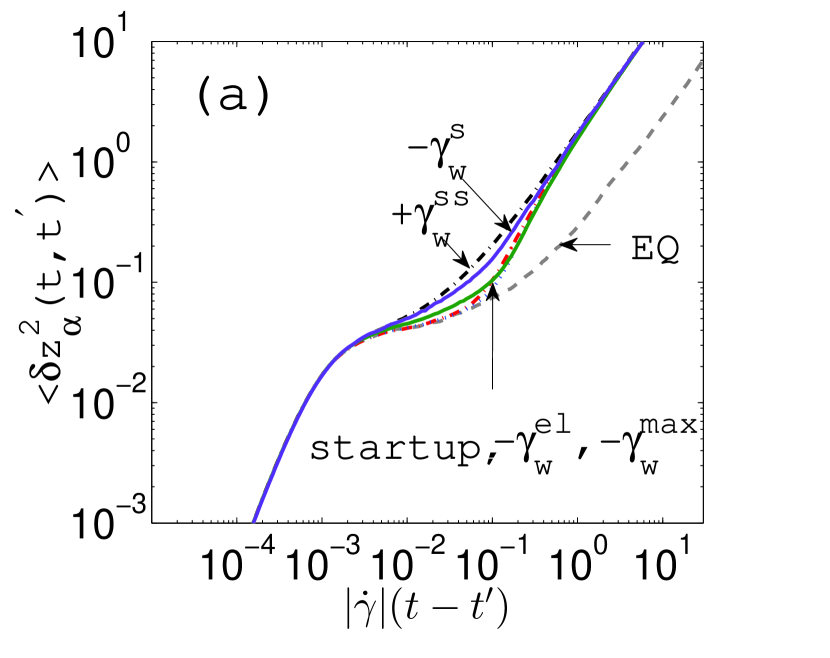
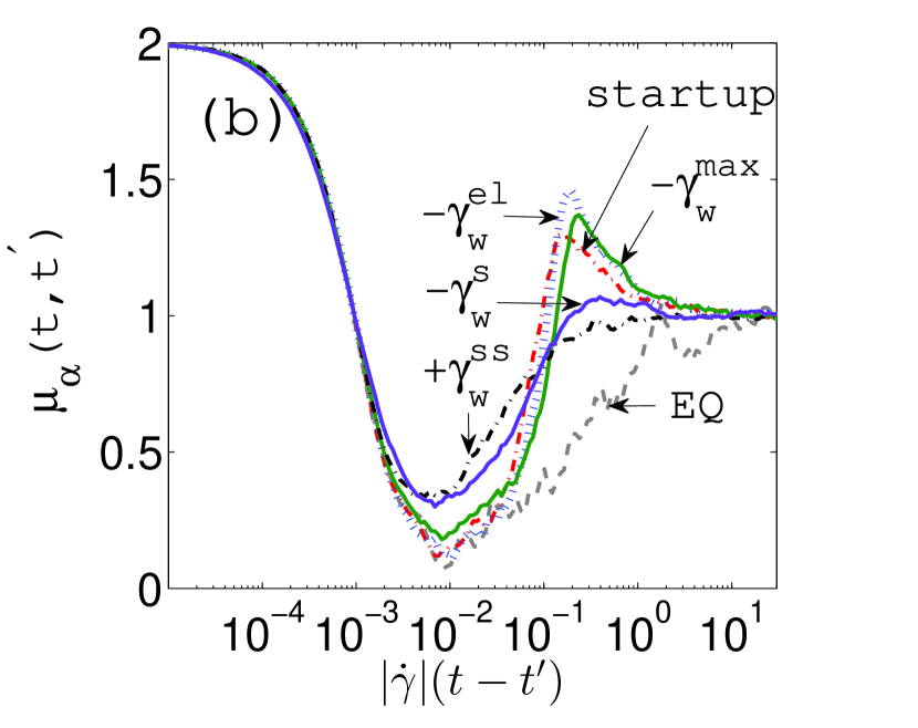
Figure 12: (a) Mean-squared displacement of B particles in the vorticity direction. Shown are the equilibrium curve for $T=0.4$ (label EQ), and transient MSDs $\delta z^{2}(t,t^{\prime})$ as a function of $|\dot{\gamma}|(t-t^{\prime})$, where $t^{\prime}$ is the time of initial flow start-up from equilibrium (EQ) respectively flow reversal according to the cases discussed in Fig. 2 (steady-state, s; elastic transient, el; strain corresponding to the overshoot, max). The equilibrium curve is shifted to coincide at short times. (b) Logarithmic derivative $\mu_{t^{\prime}}(t)=d\log\delta z^{2}(t,t^{\prime})/d\log t$ for the cases shown in (a).

A related quantity that can be intuitively interpreted is the mean-squared displacement (MSD), $\delta r^{2}(t,t^{\prime})$, of a single particle. We choose randomly a particle of species B, and show the results in Fig. 12. Here we show, in addition to the cases $t^{\prime}\ll 0$, $t^{\prime}=0$, and $t^{\prime}=t_{w}^{\text{s}}$ discussed above, also the MSDs obtained for $t^{\prime}=t_{w}^{\text{el}}$ and $t^{\prime}=t_{w}^{\text{max}}$. For simplicity, we only record the motion in the neutral direction; the MSD is then defined as $\delta r^{2}(t)=3\delta z^{2}(t)$ to match the spatially averaged MSD of the quiescent system at short times. $\delta z^{2}(t)$ is expected to become diffusive at long times, while the other components of the MSD under shear attain superdiffusive asymptotes due to (the high-density analog of) Taylor dispersion Krüger, Weysser, and Fuchs (2011).

It has been established by computer simulation and confocal microscopy studies Zausch et al. (2008, 2010) that the stress-overshoot in startup flow is accompanied by superdiffusive particle motion on intermediate time scales. This is confirmed by the startup case shown in Fig. 12: while the equilibrium MSD remains subdiffusive at all times, the transient MSD obtained for $t^{\prime}=0$ follows the equilibrium one up to a time that corresponds to a few percent strain. Then, it quickly crosses over to the diffusive regime obtained under steady-state flow. An effective exponent can be assigned to the MSD curves by taking the logarithmic derivative, $\mu(t)=d\log\delta r^{2}(t)/d\log t$. This quantity is shown in the lower panel of Fig. 12. Since the short-time motion of the simulation is ballistic, $\mu(t)=2$ holds for $t\to 0$; in the plateau region, $\mu(t)$ drops to values close to zero, and for long times, $\mu(t)=1$ indicates diffusive motion. For times where the fast increase in the $t^{\prime}=0$ MSD is seen, $\mu(t)\approx 1.3$ holds, in qualitative agreement with the simulation of Ref. [Zausch et al., 2008].

Remarkably, the correlation between stress overshoot and superdiffusive motion of the individual particles holds beyond the case of startup. In Fig. 12, we observe superdiffusive MSDs for those cases, where the corresponding stress–strain curve in Fig. 3 shows an overshoot; for the case of flow reversal in the steady state, where the stress overshoot has vanished, also only subdiffusive motion is seen in the MSD. This hints at a strong connection between the two phenomena. Such a connection can be rationalized Zausch et al. (2008) by invoking a generalized Stokes-Einstein relation: the mean-squared displacement is determined by a Mori-Zwanzig equation similar to Eq. (4). The relevant memory kernel can be approximated by the generalized time-dependent shear modulus appearing in the Green-Kubo relation for the stress, Eq. (1). Although it does not provide a sufficient condition, one sees that a memory kernel with negative portions in the MSD equations may lead to superdiffusive behavior. Both stress-overshoot and superdiffusive MSD would then arise in the same time window characterized by the strain $\gamma^{*}$.

V Conclusions

We have discussed the history-dependent response of sheared glass-forming liquids subject to shear flow whose direction is instantaneously reversed. Starting from the equilibrated liquid, application of a constant shear rate $\dot{\gamma}$ causes the resulting stress $\sigma$ to increase from zero to a steady-state value, undergoing an intermediate maximum, the stress overshoot. Flow reversal, or equivalently, application of a constant shear rate to a system that is in steady state corresponding to the flow in opposite direction, results in a stress-versus-time curve that has no maximum. At the same time, the (effective) elastic shear modulus found from the initial rate of change of the stress is lowered, and the regime in applied strain shrinks over which the behavior is described by this initial linear elastic regime. These coincident phenomena can be seen as analogous to the Bauschinger effect in simple shear flow. It should be pointed out that the original Bauschinger effect Bauschinger (1886) was discussed for metals and steels under compressional and tensile load. However, given the generality of history-dependent flow phenomena in amorphous systems, one may expect that the underlying mechanisms are related to our discussion.

We have presented a systematic investigation of the gradual change between the two cases of starting shear from a quiescent equilibrium and a sheared steady state that belongs to the opposite flow. Reversing the flow direction after an initial deformation that remains in the linear elastic regime, no change in the stress overshoot or the elastic coefficients is seen. The position of the overshoot indeed, as envisaged already by Bauschinger Bauschinger (1886), marks the end of the reversible elastic regime: at this point, plastic deformation gradually takes over, and the effective elastic coefficients drop over a small window in applied pre-strain.

Our theoretical analysis follows the integration-through-transients (ITT) scheme upon which the mode-coupling theory for colloidal rheology is based. The central physical mechanism expressed in our model is one of temporal history dependence: glass-forming liquids are visco-elastic, with a large time window $\tau$ over which the fate of past density fluctuations affects the present response. It is this history dependence that causes the Bauschinger effect and similar pre-shear-dependent phenomena in the model, rather than spatial anisotropies induced by the pre-shear (since no information on spatial variation of fluctuations is kept). This is in alignment with the microscopic MCT and molecular-dynamics simulations of the sheared thermal fluid Henrich et al. (2009); Krüger, Weysser, and Fuchs (2011), where it was found that the steady state exhibits almost isotropic (one-time) pair correlation functions. This may be different in the athermal limit. It does, however, qualitatively explain the disappearance of the stress overshoot, and our findings for the tagged-particle correlation functions and mean-squared displacements. Immediately, this discussion predicts, that inserting a waiting time between the opposing flows would cause the Bauschinger effect to weaken and go away. Any quiescent waiting period before shear-reversal would enable relaxation to proceed and would ultimately lead to startup curves from the quiescent state. When shear is started from the quiescent equilibrium configuration, nearest-neighbor cages need to be broken before the accumulated strain becomes effective in enhancing the relaxation dynamics. The critical strain is hence connected to a typical cage size; some percent of the particle diameter following a Lindemann-type criterion for melting. The sheared steady state is then characterized by less strong cages, and the directionality of the flow does not play a major role in this weakening effect. Hence, subsequent shear in the opposite direction will lead to an earlier and more gradual relaxation of correlation functions (cf. Fig. 11). The mean-squared displacements, observed to follow the unsheared equilibrium curve up to times corresponding to the critical strain in the case of startup shear, remain much closer to the sheared steady-state ones in the case of flow reversal from such a steady state. As a consequence, the sharp upturn observed for the startup case, connected to superdiffusive motion and a stress overshoot, vanishes.

At present, the analysis of the initial stress overshoot after startup of steady shear is based on a schematic model that does have a number of fit parameters whose numerical ratio has to be determined phenomenologically. However, the model is rooted in an understanding of the microscopic MCT Amann et al. (2012). In simplifying the latter to arrive at a schematic model, one aims to keep those essential features of the solutions qualitatively alike that the model shall describe; in this sense, the model used here is a minimal model containing stress-overshoot phenomena. It is important to note that the subsequent description of the fate of the stress overshoot under time-varying flow drops out naturally from the equations of motion. In this sense, the comparisons presented in Figs. 2 and 3 are qualitatively different – the first can be viewed as a model-motivated parametrization of the simulation data. The second – the comparison with the data on the Bauschinger effect – entails a parameter-free theoretical prediction.