Integrability of reductions of the discrete KdV and potential KdV equations

Abstract

We study the integrability of mappings obtained as reductions of the discrete Korteweg-de Vries (KdV) equation and of two copies of the discrete potential Korteweg-de Vries equation (pKdV). We show that the mappings corresponding to the discrete KdV equation, which can be derived from the latter, are completely integrable in the Liouville-Arnold sense. The mappings associated with two copies of the pKdV equation are also shown to be integrable.

1 Introduction

The problem of integrating differential equations goes back to the origins of calculus and its application to problems in classical mechanics. In the nineteenth century, the notion of complete integrability was provided with a solid theoretical foundation by Liouville, whose theorem gave sufficient conditions for a Hamiltonian system to be integrated by quadratures; yet only a few examples of integrable mechanical systems (mostly with a small number of degrees of freedom) were known at the time. Poincaré’s subsequent results on the non-integrability of the three-body problem seemed to indicate that many, if not most, systems should be non-integrable. Nevertheless, examples of integrable systems (and action-angle variables in particular) played an important role in the early development of quantum theory.

The theory of integrable systems only began to expand rapidly in the latter part of the twentieth century, with the discovery of the remarkable properties of the Korteweg-de Vries (KdV) equation, together with a host of other nonlinear partial differential equations that were found to be amenable to the inverse scattering technique. As well as having exact pulse-like solutions (solitons) which undergo elastic collisions, such equations could be interpreted as infinite-dimensional Hamiltonian systems, with an infinite number of conserved quantities. Moreover, it was shown that these equations admit particular reductions (e.g. to stationary solutions, or to travelling waves) which can be viewed as integrable mechanical systems with finitely many degrees of freedom. The papers in the collection [38] provide a concise and self-contained survey of the theory of integrable ordinary and partial differential equations; for a more recent set of review articles, see [21].

In the last two decades or so, there has been a more gradual development of discrete integrable systems, in the form of finite-dimensional maps [25, 5] and discrete Painlevé equations [27], as well as partial difference equations defined on lattices or quad-graphs [22, 1]. Discrete integrable systems can be obtained directly by seeking discrete analogues of particular continuous soliton equations or Hamiltonian flows [31], but they also appear independently in solvable models of statistical mechanics (see the link with the hard hexagon model in [25], for example) or quantum field theory (see [18], for instance). An important theoretical result for ordinary difference equations or maps is the fact that the Liouville-Arnold definition of integrability for Hamiltonian systems of ordinary differential equations can be extended naturally to symplectic maps [19, 4, 35], so that an appropriate modification of Liouville’s theorem holds. For lattice equations with two or three independent variables there is less theory available (especially from the Hamiltonian point of view), and the full details of the known integrable examples are still being explored, but one way to gain understanding is through the analysis of particular families of reductions.

By imposing a periodicity condition, integrable lattice equations can be reduced to ordinary difference equations (or mappings/maps) [5, 26, 15, 16]. It is believed that the reduced maps obtained from an integrable lattice equation are completely integrable in the Liouville-Arnold sense. To prove that a map is integrable one needs to find a Poisson structure together with a sufficient number of functionally independent first integrals, and then show that these integrals commute with respect to the Poisson bracket. One complication that immediately arises is that the reduced maps naturally come in families of increasing dimension, and the number of first integrals grows with the dimension. The complete integrability of some particular KdV-type maps was proved in [5], and progress has been made recently with other families of maps. For maps obtained as reductions of the equations in the Adler-Bobenko-Suris (ABS) classification [1], and for reductions of the sine-Gordon and modified Korteweg-de Vries (mKdV) equations, first integrals were given in closed form by using the staircase method and the noncommutative Vieta expansion [32, 17]. In particular, the complete integrability of mappings obtained as reductions of the discrete sine-Gordon, mKdV and potential KdV (pKdV) equations was studied in detail in [33, 34].

Given a map, the question arises as to whether it has a Poisson structure, and if so, how can one find it? In general, the answer is not known. However, for some classes of maps one can assume that in coordinates $x_{j}$ the Poisson structure is in canonical or log-canonical form, i.e. the Poisson brackets have the form $\{x_{i},x_{j}\}=\Omega_{ij}$ or $\{x_{i},x_{j}\}=\Omega_{ij}\,x_{i}x_{j}$ respectively, where $\Omega$ is a constant skew-symmetric matrix. This approach is effective for mappings obtained in the context of cluster algebras [12, 9, 10], and also applies to reductions of the lattice pKdV, sine-Gordon and mKdV equations [34]. Another approach requires the existence of a Lagrangian for the reduced map: by using a discrete analogue of the Ostrogradsky transformation, as introduced in [4], one can rewrite the map in canonical coordinates; from there one can derive a Poisson structure in the original variables.

Here we start by considering a well known integrable lattice equation, namely the discrete potential Korteweg–de Vries equation, also referred to as $H_{1}$ in the ABS list [1], which is given by

$$(u_{\ell,m}-u_{\ell+1,m+1})(u_{\ell+1,m}-u_{\ell,m+1})=1,$$ (1)

where $(\ell,m)\in\mathbb{Z}^{2}$. Early results on this equation appear in [24, 37, 5] and [22], where amongst other things it was shown that (1) leads to the continuous potential KdV equation, that is

$$\frac{\partial u}{\partial t}=\frac{\partial^{3}u}{\partial x^{3}}+3\left(\frac{\partial u}{\partial x}\right)^{2},$$ (2)

by performing a suitable continuum limit. In [5] a Lagrangian was obtained for the discrete pKdV equation (1); this can be explained using the so-called three-leg form, as in [1]. However, the associated Euler-Lagrange equation turns out to consist of two copies of the lattice pKdV equation, that is

$$u_{\ell+1,m}+u_{\ell-1,m}+\frac{1}{u_{\ell-1,m-1}-u_{\ell,m}}=u_{\ell,m+1}+u_{\ell,m-1}+\frac{1}{u_{\ell,m}-u_{\ell+1,m+1}}.$$ (3)

The latter equation, which henceforth we refer to as the double pKdV equation, is somewhat more general than (1): every solution of (1) is a solution of (3), but the converse statement does not hold. In this paper we shall be concerned with the double pKdV equation (3), rather than with (1).

Next, we introduce a new variable on the lattice, $v_{\ell,m}:=u_{\ell,m}-u_{\ell+1,m+1}$, and immediately find that, whenever $u_{\ell,m}$ is a solution of (3), $v_{\ell,m}$ satisfies

$$v_{\ell+1,m}-v_{\ell,m+1}=\frac{1}{v_{\ell,m}}-\frac{1}{v_{\ell+1,m+1}}.$$ (4)

The latter equation is known as the lattice KdV equation. Both (1) and (4) are integrable lattice equations, in the sense that they can be derived as the compatibility condition for an associated linear system, known as a Lax pair; this is discussed in section 4.

In this paper we perform the so-called $(d-1,-1)$-reduction on the discrete pKdV Lagrangian and derive the corresponding reduction of the double pKdV equation (3). This means that we consider functions $u=u_{\ell,m}$ on the lattice which have the following periodicity property under shifts:

$$u_{\ell,m}=u_{\ell+d-1,m-1}.$$ (5)

Such periodicity implies that $u$ depends on the lattice variables $\ell$ and $m$ through the combination $n=\ell+m(d-1)$ only; thus, with a slight abuse of notation, we write $u=u_{n}$. Such a reduction can be understood as a discrete analogue of the travelling wave reduction of a partial differential equation: for a function $u(x,t)$ satisfying a suitable partial differential equation such as (2), one considers solutions that are invariant under $x\to x+c\delta$, $t\to t+\delta$ for all $\delta$; such solutions depend on $x,t$ through the combination $z=x-ct$ only, corresponding to waves travelling with constant speed $c$. By analogy with the continuous case, where one obtains ordinary differential equations (with independent variable $z$) for the travelling waves, it is apparent that imposing the condition (5) in the discrete setting leads to ordinary difference equations (with independent variable $n$). Note that in the continuous case this reduction yields a one-parameter family of ordinary differential equations of fixed order (with parameter $c$), whereas in the discrete case one finds a family of ordinary difference equations whose order depends on $d$.

Here we are concerned with the complete integrability of the ordinary difference equation obtained as the $(d-1,-1)$-reduction of the double pKdV equation (3), which is equivalent to a birational map in dimension $2d$, and the associated reduction of the lattice KdV equation (4), which gives a map in dimension $d$. We begin by finding Poisson brackets for reductions of the double pKdV equation, which are then used to infer brackets for the corresponding maps obtained from lattice KdV; having found first integrals and proved Liouville integrability for the KdV maps, we are subsequently able to do the same for the double pKdV maps.

The paper is organized as follows. In section 2, we start with the discrete Lagrangian whose Euler-Lagrange equation is the double pKdV equation (3). For each $d$, we then derive a symplectic structure for the double pKdV map obtained as the $(d-1,-1)$-reduction of this discrete Euler-Lagrange equation, by using a discrete analogue of the Ostrogradsky transformation. This provides a nondegenerate Poisson bracket for each of these maps. In section 3 we present a Poisson structure for the associated map obtained as the $(d-1,-1)$-reduction of the lattice KdV equation (4), which is induced from the bracket found in section 2. The Hirota bilinear form of each of the KdV maps is also given, in terms of tau-functions, whence (via a link with cluster algebras) we derive a second Poisson structure that is compatible with the first. In section 4 we present closed-form expressions for first integrals of each reduced KdV map, and we show that they are in involution with respect to the first of the Poisson structures. This furnishes a direct proof of Liouville integrability for these KdV maps, within the framework of the papers [32] and [34]. Another proof, based on the pair of compatible Poisson brackets, is also sketched. In section 5 we return to the double pKdV maps, and present first integrals for each of them. Some of these integrals are derived from the integrals of the corresponding KdV map in the previous section, while additional commuting integrals are found using a function periodic with period $d$; this is a $d$-integral, in the sense of [13]. The paper ends with some brief conclusions, and some additional comments are relegated to an Appendix.

2 Poisson structure for the double pKdV maps

Henceforth, it is convenient to use $\widetilde{\ }$ and $\widehat{\ }$ to denote shifts in $\ell$ and $m$ directions respectively, so that $\widetilde{u}=u_{\ell+1,m}$, $\widehat{u}=u_{\ell,m+1}$, etc. It is known that all equations of the form

$$Q(u,\widetilde{u},\widehat{u},\widehat{\widetilde{u}},\alpha,\beta)=0$$ (6)

in the ABS list [1] are equivalent (up to some transformations) to the existence of an equation of so-called three-leg type, that is

$$P(u,\widetilde{u},\widehat{u},\widehat{\widetilde{u}};\alpha,\beta)\equiv\phi(u,\widehat{u},\alpha)-\phi(u,\widetilde{u},\beta)-\psi(u,\widehat{\widetilde{u}},\alpha,\beta)=0,$$ (7)

for suitable functions $\phi,\psi$, where $\alpha$ and $\beta$ are parameters; the latter leads to the derivation of a Lagrangian for each of the equations (6). In particular, for the pKdV equation (1), which is a (parameter-free) equation of the form (6), we have $\phi(u,\widetilde{u})=u+\widetilde{u}$ and $\psi(u,\widehat{\widetilde{u}})=1/(u-\widehat{\widetilde{u}})$, and using the three-leg form (7) leads to the Lagrangian

$$\mathcal{L}=\frac{1}{2}(u+\widetilde{u})^{2}-\frac{1}{2}(u+\widehat{u})^{2}-\log|u-\widehat{\widetilde{u}}|.$$ (8)

The corresponding discrete Euler-Lagrange equation is the double pKdV equation (3), which can be rewritten as

$$\widehat{\widetilde{\mathrm{J}}}-\mathrm{J}=0,\qquad\mathrm{with}\quad\mathrm{J}=\widetilde{u}-\widehat{u}-\frac{1}{(u-\widehat{\widetilde{u}})}.$$ (9)

The latter equation is more general than (1), which arises in the special case that J is identically zero.

Now setting $n=\ell+m(d-1)$, with $u$ satisfying (5), the $(d-1,-1)$-reduction applied to the Lagrangian in (8) gives $\mathcal{L}=\mathcal{L}\left(u_{n},u_{n+1},\ldots,u_{n+d}\right)$, where

$$\mathcal{L}=\frac{1}{2}(u_{n}+u_{n+1})^{2}-\frac{1}{2}(u_{n}+u_{n+d-1})^{2}-\log|u_{n}-u_{n+d}|.$$ (10)

The discrete action functional is $\mathrm{S}:=\sum_{n\in\mathbb{Z}}\mathcal{L}\left(u_{n},u_{n+1},\ldots,u_{n+d}\right)$. It yields the discrete Euler-Lagrange equation

$$\frac{\delta\mathrm{S}}{\delta u_{n}}=\sum_{r=0}^{d}\frac{\partial\mathcal{L}\left(u_{n-r},u_{n+1-r},\ldots,u_{n+d-r}\right)}{\partial u_{n}}=\sum_{r=0}^{d}\mathcal{E}^{-r}\mathcal{L}_{r}=0,$$ (11)

where $\mathcal{E}$ denotes the shift operator and $\mathcal{L}_{r}=\frac{\partial\mathcal{L}\left(u_{n},u_{n+1},\ldots,u_{n+d}\right)}{\partial u_{n+r}}$. Thus we obtain the ordinary difference equation

$$u_{n+1}-u_{n+d-1}+u_{n-1}-u_{n-d+1}-\frac{1}{u_{n}-u_{n+d}}+\frac{1}{u_{n-d}-u_{n}}=0,$$ (12)

which is precisely the $(d-1,-1)$-reduction of (3). The solutions of this equation are equivalent to the iterates of the $2d$-dimensional map

$$(u_{n-d},u_{n-d+1},\ldots,u_{n+d-1})\mapsto(u_{n-d+1},u_{n-d+2},\ldots,u_{n+d}),$$ (13)

where $u_{n+d}$ is found from equation (12).

Given a Lagrangian of first order for a classical mechanical system, the Legendre transformation produces canonical symplectic coordinates on the phase space; the Ostrogradsky transformation is the analogue of this for Lagrangians of higher order [2]. In order to derive a nondegenerate Poisson bracket for the $2d$-dimensional map, we use a discrete analogue of the Ostrogradsky transformation, as given in [4], which is a change of variables to canonical coordinates, $\left(u_{n-d},u_{n-d+1},\ldots,u_{n+d-1}\right)\to(q_{1},\ldots,q_{d},p_{1},\ldots,p_{d})$, where $q_{i}=u_{n+i-1}$, $p_{i}=\mathcal{E}^{-1}\sum_{r=0}^{d-i}\mathcal{E}^{-r}\mathcal{L}_{r+i}$. Thus, from (10), we obtain

$$q_{i} =u_{n+i-1},\quad i=1,\ldots,d;$$

$$p_{1} =-u_{n+1}+u_{n+d-1}+\frac{1}{u_{n}-u_{n+d}}=u_{n-1}-u_{n+1-d}+\frac{1}{u_{n-d}-u_{n}};$$

$$p_{i} =-u_{n+i-d}-u_{n+i-1}+\frac{1}{u_{n-d+i-1}-u_{n+i-1}},\quad i=2,\ldots,d-1;$$

$$p_{d} =\frac{1}{u_{n-1}-u_{n+d-1}}.$$

In terms of the canonical coordinates $(q_{j},p_{j})$ the map (12) is rewritten as

$$\begin{array}[]{lcllcl}q_{i}&\mapsto&q_{i+1},\quad i=1,\ldots,d-1;&q_{d}&\mapsto&q_{1}-(p_{1}+q_{2}-q_{d})^{-1};\\ p_{1}&\mapsto&p_{2}+q_{2}+q_{1};&p_{i}&\mapsto&p_{i+1},\quad i=2,\ldots,d-2;\\ p_{d-1}&\mapsto&p_{d}-q_{1}-q_{d};&p_{d}&\mapsto&p_{1}+q_{2}-q_{d}.\end{array}$$

By the general results in [4], this map is symplectic with respect to the canonical symplectic form $\sum_{j=1}^{d}\mathrm{d}p_{j}\wedge\mathrm{d}q_{j}$. Equivalently, it preserves the canonical Poisson brackets $\{p_{i},p_{j}\}=\{q_{i},q_{j}\}=0$, $\{p_{i},q_{j}\}=\delta_{ij}$.

In order to find the Poisson brackets for the coordinates $u_{n}$, we write them in terms of $(q_{j},p_{j})$. For all $0\leq i\leq d-1$, we have $u_{n+i}=q_{i+1}$, and

$$\begin{array}[]{rcl}u_{n-1}&=&q_{d}+1/p_{d}=[q_{d};p_{d}],\\ u_{n-i-1}&=&[q_{d-i};p_{d-i}+q_{d-i}+u_{n-i}]\qquad(\mathrm{for}\,\,1\leq i\leq d-2),\\ u_{n-d}&=&[q_{1};p_{1}+u_{n+1-d}-u_{n-1}],\\ \end{array}$$

which means that for $1\leq i\leq d-2$, $u_{n-i-1}$ is found recursively as

$$[q_{d-i};p_{d-i}+q_{d-i}+q_{d-i+1},p_{d-i+1}+q_{d-i+1}+q_{d-i+2},\ldots,p_{d-1}+q_{d-1}+q_{d},p_{d}],$$

while $u_{n-d}=[q_{1};p_{1}-q_{d}+q_{2}-\frac{1}{p_{d}},p_{2}+q_{2}+q_{3},\ldots,p_{d-1}+q_{d-1}+q_{d},p_{d}]$, where $[\,\,;\,]$ denotes a continued fraction. This yields the following result.

Theorem 1.

The $2d$-dimensional map given by (13) with (12) is a Poisson map with respect to the nondegenerate bracket given for $0\leq j<d-1$ by

$$\begin{array}[]{rcl}\{u_{n-d},u_{n-j-1}\}&=&0,\\ \{u_{n-d},u_{n+j}\}&=&(-1)^{j+1}(u_{n-d}-u_{n})^{2}\ldots(u_{n-d+j}-u_{n+j})^{2},\\ \{u_{n-d},u_{n+d-1}\}&=&(-1)^{d}(u_{n-d}-u_{n})^{2}\ldots(u_{n-1}-u_{n+d-1})^{2}\\ &&-(u_{n-d}-u_{n})^{2}(u_{n-1}-u_{n+d-1})^{2}.\end{array}$$ (14)

Proof.

In order to prove the first of the formulae in (2.9), we note that

$$\begin{array}[]{rl}\{u_{n-d},u_{n-r-1}\}=&\{[q_{1};p_{1}-q_{d}+q_{2}-\frac{1}{p_{d}},p_{2}+q_{2}+q_{3},\ldots,p_{d-1}+q_{d-1}+q_{d},p_{d}],\\ &[q_{d-r};p_{d-r}+q_{d-r}+q_{d-r+1},\ldots,p_{d-1}+q_{d-1}+q_{d},p_{d}]\}\\ =&\sum_{i\geq d-r}\left(\frac{\partial u_{n-d}}{\partial p_{i}}\frac{\partial u_{n-r-1}}{\partial q_{i}}-\frac{\partial u_{n-d}}{\partial q_{i}}\frac{\partial u_{n-r-1}}{\partial p_{i}}\right).\end{array}$$

Then we anticipate the next section by setting $v_{n}:=u_{n-d}-u_{n}$, to find that

$$\begin{array}[]{rcll}\frac{\partial u_{n-d}}{\partial p_{i}}&=&(-1)^{i}v_{n}^{2}\ldots v_{n+i-1}^{2},&i<d,\\ \frac{\partial u_{n-d}}{\partial p_{d}}&=&(-1)^{d}\,v_{n}^{2}\ldots v_{n+d-1}^{2}-v_{n}^{2}v_{n+d-1}^{2},&\\ \frac{\partial u_{n-d}}{\partial q_{i}}&=&(-1)^{i-1}\,v_{n}^{2}\ldots v_{n+i-2}^{2}\big{(}1-v_{n+i-1}^{2}\big{)},&i<d,\\ \frac{\partial u_{n-d}}{\partial q_{d}}&=&v_{n}^{2}+(-1)^{d-1}\,v_{n}^{2}\ldots v_{n+d-2}^{2},&\\ \frac{\partial u_{n-r-1}}{\partial p_{i}}&=&(-1)^{r+i-1-d}\,v_{n+d-r-1}^{2}\ldots v_{n+i-1}^{2},&\\ \frac{\partial u_{n-r-1}}{\partial q_{i}}&=&(-1)^{r+i-d}\,v_{n+d-r-1}^{2}\ldots v_{n+i-2}^{2}\big{(}1-v_{n+i-1}^{2}\big{)},&i<d,\\ \frac{\partial u_{n-r-1}}{\partial q_{d}}&=&(-1)^{r}\,v_{n+d-r-1}^{2}\ldots v_{n+d-2}^{2},\end{array}$$

for $i\geq d-r\geq 2$, and hence we obtain $\{u_{n-d},u_{n-r-1}\}=0$. Next, we use $\{u_{n-d},u_{n+j}\}=\{u_{n-d},q_{j+1}\}=\frac{\partial u_{n-d}}{\partial p_{j+1}}$, where $0\leq j\leq d-1$, from which the second and third formulae in (2.9) follow. ∎

3 Poisson structures and tau-functions for the KdV maps

As mentioned above, the discrete KdV equation can be derived from the double pKdV equation. This suggests that the symplectic structure given in the previous section can be used to find a Poisson structure for the $(d-1,-1)$-reduction of the discrete KdV equation. It turns out that, in addition to the bracket induced from double pKdV, each of the KdV maps has a second, independent Poisson bracket, which is obtained from a Hirota bilinear form in terms of tau-functions. The second bracket is constructed by making use of a connection with Somos recurrences and cluster algebras.

3.1 First Poisson structure from pKdV

Whenever $u_{n}$ is a solution of equation (12), $v_{n}=u_{n-d}-u_{n}$ satisfies a difference equation of order $d$, namely

$$v_{n+d-1}-v_{n+1}-\frac{1}{v_{n+d}}+\frac{1}{v_{n}}=0.$$ (15)

Alternatively, by starting from a solution of (3) with the periodicity property (5), we see that this yields a solution $v=v_{\ell,m}$ of (4) with the same periodicity, and so (writing this as $v_{n}$, with the same abuse of notation as before) it is clear that equation (15) is just the $(d-1,-1)$-reduction of the discrete KdV equation. Equivalently, the ordinary difference equation (15) corresponds to the $d$-dimensional map

$$\varphi:\quad(v_{0},v_{1},\ldots,v_{d-1})\mapsto\left(v_{1},v_{2},\ldots,v_{d-1},\frac{v_{0}}{1+v_{d-1}v_{0}-v_{1}v_{0}}\right).$$ (16)

The case $d=2$ is trivial, so henceforth we consider $d\geq 3$.

In the above, the suffix $n$ has been dropped, taking a fixed $d$-tuple $(v_{0},v_{1},\ldots,v_{d-1})$ in $d$-dimensional space. However, because the map (16) is obtained from a recurrence of order $d$, all of the formulae are invariant under simultaneous shifts of all indices by an arbitrary amount $n$, i.e. $v_{j}\to v_{n+j}$ for each $j$. For a fixed $n$, say $n=0$, the formulae in Theorem 1 define a Poisson bracket in dimension $2d$, which can be used to calculate the brackets between the quantities $v_{j}=u_{j-d}-u_{j}$ for $j=0,\ldots,d-1$. Remarkably, these brackets can be rewitten in terms of $v_{j}$ alone; in other words, these quantities form a Poisson subalgebra of dimension $d$. Hence this provides the first of two ways to endow (16) with a Poisson structure.

Theorem 2.

The $d$-dimensional map (16) preserves the Poisson bracket $\{\,,\,\}_{1}$ defined by

$${\{v_{i},v_{j}\}_{1}=\left\{\begin{array}[]{ll}(-1)^{j-i}\prod_{r=i}^{j}v_{r}^{2},&0<j-i<d-1,\\ \left(1+(-1)^{d-1}\prod_{r=1}^{d-2}v_{r}^{2}\right)v_{0}^{2}v_{d-1}^{2},&j-i=d-1.\end{array}\right.}$$ (17)

This bracket is degenerate, with one Casimir when $d$ is odd, and two independent Casimirs when $d$ is even.

The above result follows immediately from Theorem 1, apart from the statement about the Casimirs, which will be explained shortly. Here we first give a couple of examples for illustration.

Example 3.

When $d=3$ the map $\varphi$ given by (16) preserves the bracket

$$\{v_{0},v_{1}\}_{1}=-v_{0}^{2}v_{1}^{2},\quad\{v_{1},v_{2}\}_{1}=-v_{1}^{2}v_{2}^{2},\quad\{v_{0},v_{2}\}_{1}=(1+v_{1}^{2})v_{0}^{2}v_{2}^{2}.$$

This Poisson bracket has rank two, with a Casimir $\cal C$ that is also a first integral for the map, i.e. $\varphi^{*}\cal C=\cal C$ with

$${\cal C}=v_{1}-\frac{1}{v_{0}}-\frac{1}{v_{1}}-\frac{1}{v_{2}}.$$

Example 4.

When $d=4$ the map (16) preserves the bracket specified by

$$\{v_{0},v_{1}\}_{1}=-v_{0}^{2}v_{1}^{2},\quad\{v_{0},v_{2}\}_{1}=v_{0}^{2}v_{1}^{2}v_{2}^{2},\quad\{v_{0},v_{3}\}_{1}=(1-v_{1}^{2}v_{2}^{2})v_{0}^{2}v_{3}^{2},$$

where all other brackets $\{v_{i},v_{j}\}_{1}$ for $0\leq i,j\leq d-1$ are determined from skew-symmetry and the Poisson property of $\varphi$. This is a bracket of rank two, having two independent Casimirs given by

$${\cal C}_{1}=v_{1}-\frac{1}{v_{0}}-\frac{1}{v_{2}},\quad{\cal C}_{2}=v_{2}-\frac{1}{v_{1}}-\frac{1}{v_{3}},\qquad\mathrm{with}\quad\varphi^{*}{\cal C}_{1}={\cal C}_{2},\quad\varphi^{*}{\cal C}_{2}={\cal C}_{1}.$$

Remark 5.

The Casimirs ${\cal C}_{j}$ in the preceding example are 2-integrals [13], meaning that they are preserved by two iterations of the map, i.e. $(\varphi^{*})^{2}{\cal C}_{j}={\cal C}_{j}$ for $j=1,2$. The symmetric functions

$${\cal K}={\cal C}_{1}+{\cal C}_{2},\qquad{\cal K}^{\prime}={\cal C}_{1}{\cal C}_{2}$$ (18)

provide two independent first integrals.

In order to make the properties of the Poisson bracket $\{\,,\,\}_{1}$ more transparent, we introduce some new coordinates, the motivation for which should become clear from the Lax pairs in section 4.

Lemma 6.

For all $d\geq 4$, with respect to the coordinates

$$g_{0}=-1/v_{0},\qquad g_{j}=v_{j-1}-1/v_{j},\quad j=1,\ldots,d-1,$$ (19)

the first Poisson bracket for the KdV map (16) is specified by the following relations for $\nu=1$ and $0\leq i<j\leq d-1$:

$$\{g_{i},g_{j}\}_{1}=\left\{\begin{array}[]{ll}-1&\mbox{if}\ \,j-i=1,\\ 1&\mbox{if}\ \,j-i=d-1,\\ \nu/g_{0}^{2}&\mbox{if}\ \,i=1,j=d-1,\\ \ 0&\mbox{otherwise}.\end{array}\right.$$ (20)

When $d$ is odd this bracket has the Casimir

$${\cal C}=g_{0}+g_{1}+\ldots+g_{d-1}+\frac{\nu}{g_{0}},$$ (21)

while for even $d$ there are the two Casimirs

$${\cal C}_{1}=g_{0}+g_{2}+\ldots+g_{d-2},\qquad{\cal C}_{2}=g_{1}+g_{3}+\ldots+g_{d-1}+\frac{\nu}{g_{0}}.$$ (22)

Remark 7.

When $\nu=0$ the Poisson bracket (20) is just the first Poisson bracket for the dressing chain, as given by equation (13) in [36].

In terms of the coordinates $g_{j}$, the map (16) is rewritten as

$$\varphi:\quad(g_{0},g_{1},\ldots,g_{d-1})\mapsto\left(g_{1}+\frac{1}{g_{0}},g_{2},\ldots,g_{d-1},\frac{g_{0}^{2}g_{1}}{1+g_{0}g_{1}}\right).$$ (23)

Note that for the special case $d=3$, as in Example 3, part of the formula for the bracket (20) requires a slight modification, namely $\{g_{1},g_{2}\}_{1}=-1+1/g_{0}^{2}$.

3.2 Second Poisson structure from cluster algebras for tau-functions

The discrete KdV equation (4) was derived by Hirota in terms of tau-functions, via the Bäcklund transformation for the differential-difference KdV equation [14]. In Hirota’s approach, the solution of the discrete KdV equation is given in terms of a tau-function as $v=\widetilde{\tau}\widehat{\tau}/(\tau\widehat{\widetilde{\tau}})$, and at the level of the $(d-1,-1)$-reduction this becomes

$$v_{n}=\frac{\tau_{n+1}\,\tau_{n+d-1}}{\tau_{n}\,\tau_{n+d}}.$$ (24)

By direct substitution, it then follows that $v_{n}$ is a solution of (15) provided that $\tau_{n}$ satisfies the trilinear (degree three) recurrence relation

$$\begin{array}[]{rcl}\tau_{n+2d}\,\tau_{n+d-1}\,\tau_{n+1}&=&\tau_{n+2d-1}\,\tau_{n+d+1}\,\tau_{n}-\tau_{n+2d-1}\,\tau_{n+d-1}\,\tau_{n+2}\\ &&+\tau_{n+2d-2}\,\tau_{n+d+1}\,\tau_{n+1}.\end{array}$$ (25)

However, this relation can be further simplified upon dividing by $\tau_{n+1}\tau_{n+d}$, which gives the relation

$$\alpha_{n}=\frac{\tau_{n}\,\tau_{n+d+1}-\tau_{n+2}\tau_{n+d-1}}{\tau_{n+1}\,\tau_{n+d}}=\frac{\tau_{n+d-1}\,\tau_{n+2d}-\tau_{n+d+1}\tau_{n+2d-2}}{\tau_{n+d}\,\tau_{n+2d-1}}=\alpha_{n+d-1}.$$

This immediately yields relations that are bilinear (degree two) in $\tau_{n}$.

Proposition 8.

The solutions of the equation (15) are given in terms of a tau-function by (24), where $\tau_{n}$ satisfies the bilinear recurrence relation

$$\tau_{n+d+1}\,\tau_{n}=\alpha_{n}\,\tau_{n+d}\,\tau_{n+1}+\tau_{n+d-1}\,\tau_{n+2}$$ (26)

of order $d+1$, with the coefficient $\alpha_{n}$ having period $d-1$.

Apart from the presence of the periodic coefficient $\alpha_{n}$, the bilinear relation (26) has the form of a Somos-$(d+1)$ recurrence [30]. Such recurrence relations (with constant coefficients) are also referred to as three-term Gale-Robinson recurrences (after [11] and [29] respectively).

Example 9.

For $d=3$ the equation (26) is a Somos-4 recurrence with coefficients of period 2, that is $\tau_{n+4}\,\tau_{n}=\alpha_{n}\,\tau_{n+3}\,\tau_{n+1}+\tau_{n+2}^{2}$, with $\alpha_{n+2}=\alpha_{n}$. Due to the Laurent phenomenon [7], the iterates of this recurrence are Laurent polynomials, i.e. polynomials in the initial values data and their reciprocals with integer coefficients; to be precise, $\tau_{n}\in\mathbb{Z}[\alpha_{0},\alpha_{1},\tau_{0}^{\pm 1},\tau_{1}^{\pm 1},\tau_{2}^{\pm 1},\tau_{3}^{\pm 1}]$ for all $n\in\mathbb{Z}$. This means that integer sequences can be generated from a suitable choice of initial data and coefficients. For instance, with the initial values $\tau_{0}=\tau_{1}=\tau_{2}=\tau_{3}=1$ and parameters $\alpha_{0}=1$, $\alpha_{1}=2$, the Somos-4 recurrence yields an integer sequence beginning with $1,1,1,1,2,5,9,61,193,1439,13892,121853,1908467,47166783,\ldots$.

From the work of Fordy and Marsh [8], it is known that, at least in the case where the coefficients are constant, recurrences of Somos type can be generated from sequences of mutations in a cluster algebra. For the purposes of this paper, the main advantage of considering the cluster algebra is that it provides a natural presymplectic structure for the tau-functions. A presymplectic form that is compatible with cluster mutations was presented in [12], and in [10] it was explained how this presymplectic structure is preserved by the recurrences considered in [8].

Cluster algebras are a new class of commutative algebras which were introduced in [6]. Rather than having a set of generators and relations that are given from the start, the generators of a cluster algebra are defined recursively by an iterative process known as cluster mutation. For a coefficient-free cluster algebra, one starts from an initial set of generators (the initial cluster) of fixed size, which here we take to be $d+1$. If the initial cluster is denoted by $(\tau_{1},\ldots,\tau_{d+1})$, then for each index $k$ one defines the mutation in the $k$ direction to be the transformation that exchanges one of the variables to produce a new cluster $(\tau_{1}^{\prime},\ldots,\tau_{d+1}^{\prime})$ given by

$$\tau_{j}^{\prime}=\tau_{j},\quad j\neq k,\qquad\tau_{k}^{\prime}\,\tau_{k}=\prod_{j=1}^{d+1}\tau_{j}^{[b_{jk}]_{+}}+\prod_{j=1}^{d+1}\tau_{j}^{[-b_{jk}]_{+}},$$ (27)

where the exponents in the exchange relation for $\tau_{k}^{\prime}$ come from an integer matrix $B=(b_{ij})$ known as the exchange matrix, and we have used the notation $[b]_{+}=\max(b,0)$.

As well as cluster mutation, there is an associated operation of matrix mutation, which acts on the matrix $B$; the details of this are omitted here. Fordy and Marsh gave conditions under which skew-symmetric exchange matrices $B$ have a cyclic symmetry (or periodicity) under mutation, and classified all such $B$ with period 1 [8]. They also showed how this led to recurrence relations for cluster variables, by taking cyclic sequences of mutations. The requirement of periodicity puts conditions on the elements of the skew-symmetric matrix $B$, which (for a suitable labelling of indices) can be written as

$$b_{i,d+1}=b_{1,i+1},\qquad i=1,\ldots,d,$$ (28)

and

$$b_{i+1,j+1}=b_{i,j}+b_{1,i+1}[-b_{1,j+1}]_{+}-b_{1,j+1}[-b_{1,i+1}]_{+},\qquad 1\leq i,j\leq d.$$ (29)

The corresponding recurrence is defined by iteration of the map $(\tau_{1},\ldots,\tau_{d},\tau_{d+1})\mapsto(\tau_{2},\ldots,\tau_{d+1},\tau_{1}^{\prime})$ associated with the exchange relation (27) for index $k=1$, where the exponents are given by the entries $b_{1,j}$ in the first row of $B$. Moreover, given a recurrence relation of this type, the conditions (28) and (29) allow the rest of the matrix $B$ to be constructed from the exponents corresponding to the first row, and these conditions are also necessary and sufficient for a log-canonical presymplectic form $\omega$, as in (30) below, to be preserved (see Lemma 2.3 in [10]). In general this two-form is closed, but it may be degenerate.

For the case at hand, the exponents appearing in the two monomials on the right hand side of (26) specify the first row of the matrix $B$ as $(0,1,-1,0,\ldots,0,-1,1),$ and the rest of this matrix is found by applying (28) and (29). Although the foregoing discussion was put in the context of coefficient-free cluster algebras, the presence of coefficients in front of these two monomials does not affect the behaviour of the corresponding log-canonical two-form under iteration. Thus we obtain

Lemma 10.

For all $d\geq 5$, the Somos-$(d+1)$ recurrence (26) preserves the presymplectic form

$$\omega=\sum_{i<j}\frac{b_{ij}}{\tau_{i}\tau_{j}}\,\mathrm{d}\tau_{i}\wedge\mathrm{d}\tau_{j},$$ (30)

given in terms of the entries of the associated skew-symmetric exchange matrix $B=(b_{ij})$ of size $d+1$, where (with an asterisk denoting the omitted entries below the diagonal)

$$B=\left(\begin{array}[]{ccrrccrr}0&1&-1&0&\cdots&0&-1&1\\ &\ddots&2&-1&0&\cdots&1&-1\\ &&\ddots&\ddots&\ddots&\ddots&&0\\ &&&\ddots&\ddots&\ddots&\ddots&\vdots\\ &&&&\ddots&\ddots&\ddots&0\\ &&&&&\ddots&2&-1\\ &*&&&&&0&1\\ &&&&&&&0\end{array}\right).$$

Remark 11.

In each of the special cases $d=3,4$, the exchange matrix does not fit into the general pattern above. For the details of the case $d=3$, when (26) is a Somos-4 relation, see Example 2.11 in [10]; and for $d=4$ (Somos-5) see Example 1.1 in [9].

The exchange matrices being considered here are all degenerate: for $d$ odd, $B$ has a two-dimensional kernel, while for $d$ even, the kernel is three-dimensional. In the odd case, the kernel is associated with the action of a two-parameter group of scaling symmetries, namely

$$\tau_{n}\rightarrow\rho\,\sigma^{n}\,\tau_{n},\qquad\rho,\sigma\neq 0,$$ (31)

while in the even case there is the additional symmetry

$$\tau_{n}\rightarrow\xi^{(-1)^{n}}\,\tau_{n},\qquad\xi\neq 0.$$ (32)

In the theory of tau-functions such scalings are known as gauge transformations. By Lemma 2.7 in [10] (see also section 6 therein), symplectic coordinates are obtained by taking a complete set of invariants for these scaling symmetries. With a suitable choice of coordinates, denoted below by $y_{n}$, the associated symplectic maps can be written in the form of recurrences, like so:

• Odd $d$: The quantities $y_{n}=\tau_{n+2}\tau_{n}/\tau_{n+1}^{2}$ are invariant under (31), and satisfy the difference equation

  $$y_{n+d-1}\,(y_{n+d-2}\,\cdots\,y_{n+1})^{2}\,y_{n}=\alpha_{n}\,y_{n+d-2}\,\cdots\,y_{n+1}+1.$$ (33)

• Even $d$: The quantities $y_{n}=\tau_{n+3}\tau_{n}/(\tau_{n+2}\tau_{n+1})$ are invariant under both (31) and (32), and satisfy the difference equation

  $$y_{n+d-2}\,\cdots\,y_{n}=\alpha_{n}\,y_{n+d-3}y_{n+d-5}\,\cdots\,y_{n+1}+1.$$ (34)

Example 12.

Both of the cases $d=3$ and $d=4$ lead to iteration of maps in the plane with coefficients that vary periodically, namely

$$\qquad\,\,\,d=3:\qquad y_{n+2}\,y_{n+1}^{2}\,y_{n}=\alpha_{n}\,y_{n+1}+1,\qquad\mathrm{with}\quad\alpha_{n+2}=\alpha_{n},$$

$$\mathrm{and}\quad d=4:\qquad y_{n+2}\,y_{n+1}\,y_{n}=\alpha_{n}\,y_{n+1}+1,\qquad\mathrm{with}\quad\alpha_{n+3}=\alpha_{n}.$$

Remark 13.

Due to the presence of the periodic coefficients, the latter maps are not of standard QRT type [25], but they reduce to symmetric QRT maps when $\alpha_{n}=$constant. Maps in the plane of this more general type have recently been studied systematically by Roberts [28].

In general, the solutions of (33) or (34) correspond to the iterates of a symplectic map, in dimension $d-1$ or $d-2$, respectively. To be more precise, rather than just iterating a single map, each iteration depends on the coefficient $\alpha_{n}$ which varies with a fixed period (as in Proposition 8), but the same symplectic structure is preserved at each step. The appropriate symplectic form in the coordinates $y_{n}$ can be obtained from (30), and by a direct calculation the associated nondegenerate bracket is found; this is presented as follows.

Lemma 14.

For $d$ odd, each iteration of (33) preserves the nondegenerate Poisson bracket specified by

$$\{y_{i},y_{j}\}=(-1)^{j-i+1}\,y_{i}\,y_{j},\qquad 0\leq i<j\leq d-2.$$ (35)

For $d$ even, the map defined by (34) preserves the nondegenerate bracket in dimension $d-2$ given by

$$\{y_{i},y_{i\pm 1}\}=\pm\,y_{i}\,y_{i\pm 1},$$ (36)

with all other brackets $\{y_{i},y_{j}\}$ for $0\leq i<j\leq d-3$ being zero.

The bracket for the variables $y_{i}$ is the key to deriving a second Poisson structure for the KdV maps when $d$ is odd.

Theorem 15.

In the case that $d$ is odd, the map (16) preserves a second Poisson bracket, which is specified in terms of the coordinates (19) by

$$\{g_{i},g_{j}\}_{2}=(-1)^{j-i+1}\,g_{i}\,g_{j},\qquad 0\leq i<j\leq d-1.$$ (37)

Proof.

Substituting for $v_{n}$ from the formula (24) and making use of the bilinear equation (26) produces the identities

$$v_{j-1}-\frac{1}{v_{j}}=\frac{\tau_{j}(\tau_{j+1}\tau_{j+d-2}-\tau_{j-1}\tau_{j+d})}{\tau_{j+d-1}\tau_{j-1}\tau_{j+1}}=-\frac{\alpha_{j-1}\tau_{j}^{2}}{\tau_{j-1}\tau_{j+1}},$$

so that, by the definition of the symplectic coordinates $y_{j}$, $g_{j}=-\alpha_{j-1}/y_{j-1}$ for $j=1,\ldots,d-1$. A similar calculation in terms of tau-functions also yields $g_{0}=-y_{0}\,y_{1}\cdots y_{d-2}$. Noting that the coefficients $\alpha_{i}$ play the role of constants with respect to the bracket (35), this immediately implies that the induced brackets between the $g_{i}$ are

$$\{g_{i},g_{j}\}=\alpha_{i-1}\alpha_{j-1}y_{i-1}^{-2}y_{j-1}^{-2}\{y_{i-1},y_{j-1}\}=(-1)^{j-i+1}g_{i}g_{j}$$

for $1\leq i<j\leq d-1$, which agrees with (37). By making use of the preceding formula for $g_{0}$ in terms of $y_{i}$, the brackets $\{g_{0},g_{j}\}$ follow in the same way. ∎

Remark 16.

The bracket (37) is the same as the quadratic bracket for the dressing chain (for the case where all parameters $\beta_{i}$ are zero in [36]). It has the Casimir

$${\cal C}^{*}=g_{0}\,g_{1}\cdots g_{d-1},$$ (38)

which is also given in terms of the coefficients of the bilinear equation (26) by ${\cal C}^{*}=-\prod_{j=0}^{d-2}\alpha_{j}$.

The case where $d$ is even is slightly more complicated, because we do not have a direct way to derive a second Poisson bracket in terms of the coordinates $g_{i}$ (or equivalently $v_{i}$). The reason for this difficulty is that, from the tau-function expressions, although the quantities $g_{i}$ remain the same under the action of the two-parameter symmetry group (31), they are not invariant under the additional scaling (32), but rather they transform differently according to the parity of the index $i$:

$$g_{i}\longrightarrow\xi^{\pm 4}\,g_{i}\qquad\mathrm{for}\quad\mathrm{even/odd}\quad i.$$ (39)

In order to obtain a fully invariant set of variables, we introduce a projection $\pi$ from dimension $d$ to dimension $d-1$:

$$\pi:\quad f_{i}=g_{i}g_{i+1},\qquad i=0,\ldots,d-2.$$

By regarding the new coordinates $f_{i}$ as functions of the $g_{j}$, we get an induced map $\varphi^{\prime}$ in dimension $d-1$, which is compatible with $\varphi$ in the sense that $\varphi\cdot\pi=\pi\cdot\varphi^{\prime}$; this has the form

$$\begin{array}[]{rl}\varphi^{\prime}:&\quad(f_{0},f_{1},\ldots,f_{d-2})\\ &\mapsto\left(f_{1}(1+f_{0}^{-1}),f_{2},\ldots,f_{d-2},\frac{f_{0}f_{2}\cdots f_{d-2}}{(1+f_{0}^{-1})f_{1}f_{3}\cdots f_{d-3}}\right).\end{array}$$ (40)

In terms of tau-functions, the quantities $f_{i}$ are invariant under the action of the full three-parameter group of gauge transformations, which means that they can be expressed as functions of the invariant symplectic coordinates $y_{n}$, and hence we can derive a Poisson bracket for them.

Theorem 17.

In the case that $d$ is even, the map (40) preserves a Poisson bracket, which is specified in terms of the coordinates $f_{i}$ by

$$\{f_{i},f_{i\pm 1}\}_{2}=\pm\,f_{i}\,f_{i\pm 1},$$ (41)

with all other brackets $\{f_{i},f_{j}\}_{2}$ for $0\leq i<j\leq d-2$ being zero.

Proof.

Following the proof of Theorem 15, we have $g_{i}g_{i+1}=\alpha_{i-1}\alpha_{i}\tau_{i}\tau_{i+1}/(\tau_{i-1}\tau_{i+2})$, whence, in terms of the symplectic coordinates for (34), we have $f_{i}=\alpha_{i-1}\alpha_{i}/y_{i-1}$ for $i=1,\ldots,d-2$. A similar calculation yields a slightly different formula for index $i=0$: $f_{0}=\alpha_{0}\,y_{1}y_{3}\cdots y_{d-3}$, and then the Poisson brackets (36) between the $y_{j}$ directly imply that the brackets (41) hold between the $f_{i}$. ∎

Remark 18.

The bracket (41) has the Casimir

$${\cal C}^{*}=f_{0}\,f_{2}\cdots f_{d-2},$$ (42)

which is also given in terms of the coefficients of the bilinear equation (26) by ${\cal C}^{*}=\prod_{j=0}^{d-2}\alpha_{j}$.

It may be unclear why there is the suffix $2$ on the bracket in (41), since we have not yet provided another Poisson bracket for the map (40). However, as will be explained in the next section, when $d$ is even the quantities $f_{i}$ form a Poisson subalgebra for the bracket $\{\,,\,\}_{1}$ of Theorem 2. As will also be explained, the brackets $\{\,,\,\}_{1}$ and $\{\,,\,\}_{2}$ are compatible (in the sense that any linear combination of them is also a Poisson bracket), which means that a standard bi-Hamiltonian argument can be used to show Liouville integrability of the maps for either odd or even $d$.

4 First integrals and integrability of the KdV maps

The purpose of this section is to prove the following result.

Theorem 19.

For each $d\geq 3$, the map (16) is completely integrable in the Liouville sense.

Recall that, for a Poisson map $\varphi$ in dimension $d$, Liouville integrability means that there should be $k$ Casimirs invariant under the map, so that the $(d-k)$-dimensional symplectic leaves of the Poisson bracket are preserved by $\varphi$, plus an additional $\frac{1}{2}(d-k)$ independent first integrals that are in involution with respect to the bracket. For the particular map in question, there is always the Poisson bracket $\{\,,\,\}_{1}$, and from Lemma 6 this has either one or two Casimirs, with symplectic leaves of dimension $d-1$ or $d-2$, for odd/even $d$ respectively; hence an additional $\lfloor\frac{1}{2}(d-1)\rfloor$ first integrals are required in this case.

For the lowest values $d=3,4$, it is straightforward to verify complete integrability, since in those cases only one extra first integral is required, apart from the Casimirs of $\{\,,\,\}_{1}$. When $d=3$, as in Example 3, the Casimir $\cal C$ is preserved by $\varphi$; the quantity ${\cal C}^{*}$ in (38), which is the Casimir of the second bracket, is also a first integral. Similarly, for $d=4$, the two Casimirs in Example 4 provide the two first integrals (18), which are themselves Casimirs; the quantity ${\cal C}^{*}=f_{0}f_{2}=g_{0}g_{1}g_{2}g_{3}$, as in (42), provides the extra first integral.

Example 20.

For $d=3$, each of the first integrals ${\cal C}$, ${\cal C}^{*}$ of the map (16) define surfaces in three dimensions, given by

$$\begin{array}[]{rcl}XY^{2}Z-{\cal C}\,XYZ-XY-YZ-ZX&=&0,\\ XY^{2}Z+{\cal C}^{*}\,XYZ-XY-YZ+1&=&0,\end{array}$$

respectively, in terms of coordinates $(X,Y,Z)\equiv(v_{n},v_{n+1},v_{n+2})$. These two surfaces intersect in a curve of genus one, found explicitly by eliminating the variable $Z$ above; this yields the biquadratic

$$({\cal C}+{\cal C}^{*})\,X^{2}Y^{2}+(X+Y)(XY-1)-{\cal C}\,XY=0.$$ (43)

The embedding of such a curve in three dimensions can be seen from the orbit plotted in Figure 1.

For higher values of $d$, it is not so obvious how to proceed, but the correct number of additional first integrals can be obtained by constructing a Lax pair for the map, as we now describe.

4.1 Lax pairs and monodromy

The discrete KdV equation (4) is known to be integrable in the sense that it arises as the compatibility condition for a pair of linear equations. In [23], a scalar Lax pair is given as follows:

$$\widehat{\widetilde{\phi}}=v\widetilde{\phi}+\lambda\phi,\qquad\widehat{\phi}=\widetilde{\phi}+\frac{1}{v}\phi.$$

Upon introducing the vector $\Phi:=\left(\begin{array}[]{c}\widetilde{\phi}\\ {\phi}\end{array}\right)$, the latter pair of scalar equations leads to a Lax pair in matrix form, namely

$$\widetilde{\Phi}={\bf L}\Phi,\qquad\widehat{\Phi}={\bf M}\Phi,\qquad\mathrm{with}\quad{\bf L}=\begin{pmatrix}v-\frac{1}{\widetilde{v}}&\lambda\\ 1&0\end{pmatrix},\quad{\bf M}=\begin{pmatrix}v&\lambda\\ 1&\frac{1}{v}\end{pmatrix}.$$ (44)

Equation (4) is equivalent to the compatibility condition for the linear system (44), that is

$$\widehat{{\bf L}}\,{\bf M}=\widetilde{{\bf M}}\,{\bf L}.$$ (45)

Note that the matrix ${\bf L}$ is associated with shifts in the $\ell$ (horizontal) direction, and ${\bf M}$ with shifts in the $m$ (vertical) direction.

First integrals of each KdV map (16) can be found by using the staircase method [5, 26, 15, 16]. For the $(d-1,-1)$-reduction, a staircase on the $\mathbb{Z}^{2}$ lattice is built from paths consisting of $d-1$ horizontal steps and one vertical step. Taking an ordered product of Lax matrices along the staircase yields the monodromy matrix

$$\mathcal{{L}}_{n}={\bf M}_{n}^{-1}\,{\bf L}_{n+d-2}\cdots{\bf L}_{n},$$ (46)

corresponding to $d-1$ steps to the right ($\ell\to\ell+1$) and one step down ($m\to m-1$), where ${\bf L}\to{\bf L}_{n}$ and ${\bf M}\to{\bf M}_{n}$ under the reduction. As a consequence of (45), the identity ${\bf L}_{n+d-1}{\bf M}_{n}={\bf M}_{n+1}{\bf L}_{n}$ holds, which implies that $\mathcal{L}_{n}$ satisfies the discrete Lax equation

$$\mathcal{L}_{n+1}\,{\bf L}_{n}={\bf L}_{n}\,\mathcal{L}_{n}.$$ (47)

The latter holds if and only if $v_{n}$ satisfies the difference equation (15). Since (47) means that the spectrum of $\mathcal{L}_{n}$ is invariant under the shift $n\to n+1$, first integrals for the KdV map can be constructed from the trace of the monodromy matrix (or powers thereof), which can be expanded in the spectral parameter $\lambda$.

For convenience, we conjugate $\mathcal{L}_{n}$ in (46) by ${\bf M}_{n}$ and multiply by an overall factor of $\lambda-1$, which (upon setting $n=0$) gives a modified monodromy matrix

$$\mathcal{L}^{\dagger}={\bf L}^{\dagger}_{d-1}\cdots{\bf L}^{\dagger}_{1}\,{\bf L}^{\dagger}_{0},$$ (48)

where

$${\bf L}^{\dagger}_{i}={\bf L}_{i-1}=\left(\begin{array}[]{cc}g_{i}&\lambda\\ 1&0\end{array}\right),\,i=1,\ldots,d-1,\quad\mathrm{but}\,\,{\bf L}^{\dagger}_{0}=\left(\begin{array}[]{cc}g_{0}&\lambda\\ 1&\frac{\nu}{g_{0}}\end{array}\right)\,\mathrm{with}\,\,\nu=1.$$

Thus we see the origin of the coordinates $g_{i}$ introduced in Lemma 6: they are the $(1,1)$ entries in the Lax matrices that make up the monodromy matrix. We have already mentioned a connection with the dressing chain at the level of the Poisson brackets, but it can be seen more directly here: up to taking an inverse and inserting a spectral parameter, when $\nu=0$ the expression (48) reduces to the monodromy matrix for the dressing chain found in [10]. The parameter $\nu$ can be regarded as introducing inhomogeneity into the chain at $i=0$ (and for $\nu\neq 0$ it is always possible to rescale so that $\nu=1$).

With the introduction of another spectral parameter $\mu$, we consider the characteristic polynomial of $\mathcal{L}^{\dagger}$, which defines the spectral curve

$$\chi(\lambda,\mu):=\det(\mathcal{L}^{\dagger}-\mu\,1)=\mu^{2}-{\cal P}(\lambda)\,\mu+(\nu-\lambda)(-\lambda)^{d-1}=0,$$ (49)

with ${\cal P}(\lambda)=\mathrm{tr}\,\mathcal{L}^{\dagger}$. This curve in the $(\lambda,\mu)$ plane is invariant under the KdV map (16), and the trace of $\mathcal{L}^{\dagger}$ provides the polynomial ${\cal P}$ whose non-trivial coefficients are first integrals of the map.

Example 21.

When $d=3$ the spectral curve is of genus one, given by $\mu^{2}-({\cal C}^{*}+{\cal C}\lambda)\,\mu+(\nu-\lambda)\lambda^{2}=0.$ For $\nu=1$ this is isomorphic to the biquadratic curve (43) corresponding to the intersection of the level sets of ${\cal C}$ and ${\cal C}^{*}$.

Example 22.

When $d=4$ the spectral curve also has genus one, being given by $\mu^{2}-(I_{0}+I_{1}\,\lambda+2\lambda^{2})\,\mu-(\nu-\lambda)\lambda^{3}=0$, with coefficients expressed in terms of $g_{i}$ by

$$I_{0}={\cal C}^{*}=g_{0}g_{1}g_{2}g_{3},\qquad I_{1}={\cal K}^{\prime}-\nu=g_{0}g_{1}+g_{1}g_{2}+g_{2}g_{3}+g_{3}g_{0}+\nu\,\frac{g_{2}}{g_{0}}.$$

In the next subsection, we will show how, for each $d$, expanding the trace of the monodromy matrix in powers of $\lambda$ gives the polynomial ${\cal P}$ of degree $\lfloor d/2\rfloor$. This implies that the hyperelliptic curve $\chi(\lambda,\mu)=0$ as in (49) has genus $\lfloor\frac{1}{2}(d-1)\rfloor$. Thus we expect that the (real, compact) Liouville tori for the KdV map should be identified with (a real component of) the Jacobian variety of this curve, since their dimensions coincide, and the map should correspond to a translation on the Jacobian.

4.2 Direct proof from the Vieta expansion

In order to calculate the trace of the monodromy matrix explicitly, we split the Lax matrices as

$${\bf L}^{\dagger}_{i}=\lambda\begin{pmatrix}0&1\\ 0&0\end{pmatrix}+\begin{pmatrix}g_{i}&0\\ 1&0\end{pmatrix}=\lambda\,{\bf X}+{\bf Y}_{i},\qquad i=1,\ldots d-1,$$ (50)

and similarly for ${\bf L}^{\dagger}_{0}$. This splitting fits into the framework of [32], with the coefficient of $\lambda$ being the same nilpotent matrix ${\bf X}$ in each case, and allows the application of the so-called Vieta expansion.

Recall that, in the noncommutative setting, the Vieta expansion is given by the formula

$$\prod_{i=a}^{\overset{\curvearrowleft}{b}}(\lambda{\bf X}_{i}+{\bf Y}_{i}):=(\lambda{\bf X}_{b}+{\bf Y}_{b})\ldots(\lambda{\bf X}_{a}+{\bf Y}_{a})=\sum_{r=0}^{b-a+1}\lambda^{r}{\bf Z}^{a,b}_{r},$$ (51)

where

$${\bf Z}^{a,b}_{r}=\sum_{a\leq i_{1}<i_{2}<\cdots<i_{r}\leq b}{\bf Y}_{b}{\bf Y}_{b-1}\cdots{\bf Y}_{i_{r}+1}{\bf X}_{i_{r}}{\bf Y}_{i_{r}-1}\cdots{\bf Y}_{i_{1}+1}{\bf X}_{i_{1}}{\bf Y}_{i_{1}-1}\cdots{\bf Y}_{a}.$$

In the case at hand, we have ${\bf X}_{i}={\bf X}$ for all $i$, and by writing the monodromy matrix in the form (51), we can use Lemma 8 in [32] to expand the trace as

$${\cal P}(\lambda)={\mathrm{t}r}\,\mathcal{L}^{\dagger}=\sum_{r=0}^{\lfloor d/2\rfloor}I_{r}\,\lambda^{r},$$ (52)

where the first integrals of the KdV map are given by the closed-form expression

$$I_{r}=\Psi^{1,d-3}_{r-1}+g_{0}\Psi^{1,d-4}_{r-1}+\left(g_{d-1}+\frac{\nu}{g_{0}}\right)\Psi^{2,d-3}_{r-1}+\Psi^{2,d-4}_{r-2}+g_{0}g_{d-1}\Psi^{1,d-3}_{r},$$ (53)

with

$$\Psi^{a,b}_{r}=\prod_{i=a}^{b+1}g_{i}\,\left(\sum_{a\leq i_{1}<i_{1}+1<i_{2}\ldots<i_{r}\leq b}\prod_{j=1}^{r}\frac{1}{g_{i_{j}}g_{i_{j}+1}}\right).$$ (54)

The explicit form of these integrals mean that it is possible to give a direct verification that they are in involution, which is almost identical to the proof of Theorem 13 in [34].

Proposition 23.

The first integrals (53) of the KdV map Poisson commute with respect to the bracket $\{\,,\,\}_{1}$ in (17).

Proof.

Writing the Poisson structure in terms of the coordinates $g_{i}$ as in Lemma 6, we see that (up to an overall factor of $-1$) the brackets $\{g_{i},g_{j}\}_{1}$ in (20) for $1\leq i,j\leq d-2$ are identical to the brackets between the coordinates $c_{i}$ given by equation (46) in [34]. The polynomial functions given by (54) are the same as in the latter reference, and the particular functions $\Psi^{a,b}_{r}$ that appear in the formula (53) only depend on $g_{i}$ for $1\leq i\leq d-2$. This implies that the brackets between these functions are the same as those given in Lemma 11 and Corollary 12 in [34], whence it is straightforward to verify that $\{I_{r},I_{s}\}_{1}=0$ for $0\leq r,s\leq\lfloor d/2\rfloor$. ∎

In order to complete the proof of Theorem 19, it only remains to check that there are sufficiently many independent integrals.

For odd $d$, the leading ($\nu=0$) part of the first integral $I_{r}$ is a cyclically symmetric, homogeneous function of degree $d-2r$ in the $g_{i}$, being identical to the independent integrals of the dressing chain in [36] (for parameters $\beta_{i}=0$), with terms of each odd degree appearing for $r=0,\ldots,\frac{d-1}{2}$. Hence these functions are also independent in the case $\nu\neq 0$, corresponding to the addition of a rational term with $g_{0}$ in the denominator, which is linear in $\nu$ and of degree $d-2r-2$ in the $g_{i}$. This means that there are $\deg{\cal P}=(d-1)/2+1$ independent integrals, of which the last one is $I_{(d-1)/2}={\cal C}$, the Casimir of the bracket $\{\,,\,\}_{1}$, as given in (21).

When $d$ is even, the leading ($\nu=0$) part of $I_{r}$ has the same structure, with terms of each even degree $d-2r$ appearing for $r=0,\ldots,\frac{d}{2}-1$, but for all $\nu$ the last one is trivial: $I_{d/2}=2$. Thus the coefficients of $\cal P$ provide only $\frac{d}{2}$ independent first integrals. The last non-trivial coefficient is a Casimir of $\{\,,\,\}_{1}$, given by $I_{d/2-1}={\cal C}_{1}{\cal C}_{2}-\nu$, in terms of the two Casimirs in (22), and the Casimir ${\cal C}_{1}+{\cal C}_{2}$ provides one extra first integral, as required.

In the next subsection, we outline another proof of Theorem 19, based on the bi-Hamiltonian structure obtained from the two Poisson brackets $\{\,,\,\}_{1}$ and $\{\,,\,\}_{2}$.

4.3 Proof via the bi-Hamiltonian structure

As an alternative to the direct calculation of brackets between the first integrals (53), the two Poisson brackets can be used to show complete integrability, with a suitable Lenard-Magri chain; this is a standard method for bi-Hamiltonian systems [20]. This approach applies immediately to the coordinates $g_{i}$ when $d$ is odd and the brackets are given by (20) and (37); but minor modifications are required to apply it to the coordinates $f_{i}$ when $d$ is even.

For $d$ odd, the first observation to make is that, just as in the case of the dressing chain ($\nu=0$), the brackets $\{\,,\,\}_{1}$ and $\{\,,\,\}_{2}$ are compatible with each other, in the sense that their sum, and hence any linear combination of them, is also a Poisson bracket. Thus these two compatible brackets form a bi-Hamiltonian structure for the KdV map $\varphi$. A pencil of Poisson brackets is defined by the bivector field ${\tt P}_{2}-\lambda\,{\tt P}_{1}$, where ${\tt P}_{j}$ denotes the bivector corresponding to $\{\,,\,\}_{j}$ for $j=1,2$. (In fact, since it defines a bracket for all $\lambda$ and $\nu$, this gives three compatible Poisson structures.) Then, by a minor adaptation of Theorem 4.8 in [10] (which, up to rescaling by a factor of 2, is the special case $\lambda=-1$ and $\nu=0$) we see that the trace of the monodromy matrix is a Casimir of the Poisson pencil, or in other words

$$({\tt P}_{2}-\lambda\,{\tt P}_{1})\,\lrcorner\,\mathrm{d}{\cal P}(\lambda)=0.$$ (55)

Expanding this identity in powers of $\lambda$ yields a finite Lenard-Magri chain, starting with $I_{0}={\cal C}^{*}$, the Casimir of the bracket $\{\,,\,\}_{2}$ (as in Remark 16), and ending with $I_{(d-1)/2}={\cal C}$, the Casimir of the bracket $\{\,,\,\}_{1}$ (as in Lemma 6): ${\tt P}_{2}\,\lrcorner\,\mathrm{d}I_{0}=0,{\tt P}_{2}\,\lrcorner\,\mathrm{d}I_{1}={\tt P}_{1}\,\lrcorner\,\mathrm{d}I_{0},\ldots{\tt P}_{2}\,\lrcorner\,\mathrm{d}I_{r}={\tt P}_{1}\,\lrcorner\,\mathrm{d}I_{r-1},\ldots{\tt P}_{1}\,\lrcorner\,\mathrm{d}I_{(d-1)/2}=0$. It then follows, by a standard inductive argument, that $\{I_{r},I_{s}\}_{1}=0=\{I_{r},I_{s}\}_{2}$ for $0\leq r,s\leq(d-1)/2$. Hence we see that Proposition 23 is a consequence of the bi-Hamiltonian structure in this case.

In the case where $d$ is even, a slightly more indirect argument is necessary, making the projection $\pi$ and working with the map $\varphi^{\prime}$ in dimension $d-1$, as given by (40). The main ingredient required is the expression for the relations between the coordinates $f_{i}$ for $i=0,\ldots,d-2$ with respect to the first bracket. The case $d=4$ is special, so we do this example first before summarizing the general case.

Example 24.

For $d=4$, we use Lemma 6 to calculate

$$\begin{array}[]{rcl}\{f_{0},f_{1}\}_{1}=\{g_{0}g_{1},g_{1}g_{2}\}_{1}&=&\{g_{0},g_{1}\}_{1}g_{1}g_{2}+g_{1}(\{g_{0},g_{2}\}_{1}g_{1}+g_{0}\{g_{1},g_{2}\}_{1})\\ &=&-g_{1}g_{2}-g_{0}g_{1}=-f_{0}-f_{1},\end{array}$$

and similar calculations show that

$$\{f_{0},f_{2}\}_{1}=f_{1}-\frac{f_{0}f_{2}}{f_{1}}+\nu\,\frac{f_{1}}{f_{0}},\qquad\{f_{1},f_{2}\}_{1}=-f_{1}-f_{2}+\nu\,\frac{f_{1}^{2}}{f_{0}^{2}},$$

which implies that $f_{0},f_{1},f_{2}$ generate a three-dimensional Poisson subalgebra for the bracket $\{\,,\,\}_{1}$. It follows that (40) is a Poisson map (in three dimensions) with respect to the restriction of this bracket to the subalgebra. Moreover, the restricted bracket $\{\,,\,\}_{1}$ for the $f_{i}$ is compatible with the bracket $\{\,,\,\}_{2}$ given by (41) with $d=4$. The coefficients of the corresponding spectral curve, as in Example 22, can be written as functions of the $f_{i}$, i.e.

$$I_{0}=f_{0}f_{2},\qquad I_{1}=f_{0}+f_{1}+f_{2}+\frac{f_{0}f_{2}}{f_{1}}+\nu\,\frac{f_{1}}{f_{0}},$$

and these generate the short Lenard-Magri chain $\{\,\cdot\,,I_{0}\}_{2}=0$, $\{\,\cdot\,,I_{1}\}_{2}=\{\,\cdot\,,I_{0}\}_{1}$, $\{\,\cdot\,,I_{1}\}_{1}=0$.

Theorem 25.

For all even $d\geq 6$, the first Poisson structure for the KdV map (16) reduces to a bracket for the coordinates $f_{i}=g_{i}\,g_{i+1}$, as specified by the following relations for $\nu=1$ and $0\leq i<j\leq d-2$:

$$\{f_{i},f_{j}\}_{1}=\left\{\begin{array}[]{ll}-f_{i}-f_{i+1}&\mbox{if}\ \,j-i=1,\\ \\ -\frac{f_{i}f_{i+2}}{f_{i+1}}&\mbox{if}\ \,j-i=2,\\ \\ \frac{f_{1}f_{3}\cdots f_{d-3}}{f_{2}f_{4}\cdots f_{d-4}}\left(1+\frac{\nu}{f_{0}}\right)&\mbox{if}\ j-i=d-2,\\ \\ \nu\,\frac{f_{1}^{2}f_{3}\cdots f_{d-3}}{f_{0}^{2}f_{2}\cdots f_{d-4}}&\mbox{if}\ i=1,j=d-2,\\ \\ 0&\mbox{otherwise}.\end{array}\right.$$ (56)

This Poisson bracket is preserved by the map (40).

The rest of the argument proceeds as for $d$ odd: the brackets $\{\,,\,\}_{1}$ and $\{\,,\,\}_{2}$ (as given in (56) and (41) respectively) are compatible with each other, so they provide a bi-Hamiltonian structure for $\varphi^{\prime}$ in dimension $d-1$. Letting ${\tt P}_{j}^{\prime}$ for $j=1,2$ denote the corresponding Poisson bivector fields, the analogue of (55) can then be verified: $({\tt P}_{2}^{\prime}-\lambda\,{\tt P}_{1}^{\prime})\,\lrcorner\,\mathrm{d}{\cal P}(\lambda)=0$. It should be noted that the latter identity is well-defined in the $(d-1)$-dimensional space with coordinates $f_{i}$: the trace of the monodromy matrix is invariant under the scaling symmetry (39), hence all of the first integrals $I_{r}$ can be written as functions of the variables $f_{i}$. In this case, the Lenard-Magri chain begins with $I_{0}={\cal C}^{*}$, the Casimir of $\{\,,\,\}_{2}$ (as in Remark 18), and ends with a Casimir of the bracket $\{\,,\,\}_{1}$, namely $I_{d/2-1}={\cal C}_{1}{\cal C}_{2}-\nu$ (which is well-defined in terms of $f_{i}$). Thus it follows that the integrals $I_{r}$ are in involution with respect to both brackets for the $f_{i}$, and this result extends to the bracket $\{\,,\,\}_{1}$ when it is lifted to $d$ dimensions (in terms of $g_{i}$, or equivalently $v_{i}$).

5 First integrals and integrability of the double pKdV maps

In this section, we go back to the $(d-1,-1)$-reduction of the double pKdV equation (3). This reduction yields the difference equation (12), and in section 2 we showed how writing this as the discrete Euler-Lagrange equation (11) led to a symplectic structure for the corresponding $2d$-dimensional map (13). It is easy to see that the first integrals (53) of the KdV map also provide first integrals for equation (12) by writing $v_{i}=u_{i-d}-u_{i}$ for $i=0,\ldots,d-1$. However, the total number of independent integrals for (16) is only $\lfloor d/2\rfloor+1$, which is not enough for complete integrability of the $2d$-dimensional symplectic map (13). Here we will show how to construct sufficiently many additional integrals, leading to a proof of the following result.

Theorem 26.

For all $d\geq 3$, the $2d$-dimensional map given by (13) with (12) is completely integrable in the Liouville sense.

The proof of the above, given in subsection 5.1 below, relies on the observation that equation (12) can be rewritten as

$$u_{n+1}-u_{n+d-1}-\frac{1}{u_{n}-u_{n+d}}=u_{n-d+1}-u_{n-1}-\frac{1}{u_{n-d}-u_{n}},$$

from which we see that

$$u_{n-d+1}-u_{n-1}-\frac{1}{u_{n-d}-u_{n}}=J_{n},\qquad\mathrm{with}\quad J_{n+d}=J_{n}.$$ (57)

Thus the function $J_{n}$ is a $d$-integral (in the sense of [13]) for the double pKdV map (13): for any $n$ it can be viewed as a function on the $2d$-dimensional phase space with coordinates $(u_{-d},\ldots,u_{d-1})$, and under shifting $n$ it is periodic with period $d$. This implies that any cyclically symmetric function of $J_{0},J_{1},\ldots,J_{d-1}$ is a first integral for equation (12). As we shall see, for the corresponding map (13) this has the further consequence that it is superintegrable, in the sense that it has more than the number of independent integrals required for Liouville’s theorem.

Remark 27.

For the $(d-1,-1)$-reduction, the observation that (57) holds can be seen as a direct consequence of the fact that (3) can be rewritten as (9). An analogous observation applies to the $(s_{1},-s_{2})$-reduction of (3), where $n=s_{2}\ell+s_{1}m$, and in (9) one has $\mathrm{J}\to J_{n}$ with $J_{n+s_{1}+s_{2}}=J_{n}$.

5.1 Construction of integrals in involution

In order to construct additional integrals, we need to calculate the Poisson brackets between the $J_{i}$, as well as their brackets with the $v_{j}$; together these generate a Poisson subalgebra for the bracket in Theorem 1, as described by the next two lemmata.

Lemma 28.

With respect to the nondegenerate Poisson bracket specified by (14), the quantities $J_{i}$ defined in (57) and $v_{j}=u_{j-d}-u_{j}$ Poisson commute, i.e.

$$\{J_{i},v_{j}\}=0,\qquad 0\leq i,j\leq d-1.$$ (58)

Proof.

For $0<j<d-1$ we have

$$\begin{array}[]{rcl}\{J_{0},v_{j}\}&=&\{u_{-d+1}-u_{-1}-v_{0}^{-1},v_{j}\}=\{u_{-d+1}-u_{-1},u_{j-d}-u_{j}\}+v_{0}^{-2}\{v_{0},v_{j}\}\\ &=&-\{u_{-d+1},u_{j}\}+v_{0}^{-2}\,(-1)^{j}\prod_{r=0}^{j}v_{r}^{2}=0,\end{array}$$

where we have used (17) as well as Theorem 1. Similar calculations show that $\{J_{0},v_{0}\}=0=\{J_{0},v_{d-1}\}$, and, since the bracket is preserved by the double pKdV map (13), the vanishing of all the other brackets $\{J_{i},v_{j}\}$ follows by shifting indices. ∎

Lemma 29.

The Poisson brackets between the $d$-integrals $J_{n}$ are specified by

$$\{J_{i},J_{j}\}=\left\{\begin{array}[]{ll}1,&\mbox{if}\ j-i=1,\\ -1,&\mbox{if}\ j-i=d-1,\\ 0,&\mbox{otherwise},\end{array}\right.$$ (59)

for $0\leq i<j\leq d-1$.

Proof.

Once again, from the behaviour under shifting indices, it is enough to verify the brackets for $i=0$ and $1\leq j\leq d-1$. Expanding the left hand side of (59), and using Lemma 28, we obtain

$$\begin{array}[]{rcl}\{J_{0},J_{j}\}&=&\{J_{0},u_{j-d+1}-u_{j-1}-v_{j}^{-1}\}\\ &=&\{u_{-d+1}-u_{-1}-(u_{-d}-u_{0})^{-1},u_{j-d+1}-u_{j-1}\}\\ &=&-\{u_{-d+1},u_{j-1}\}+(u_{-d}-u_{0})^{-2}\,\Big{(}\{u_{-d},u_{j-d+1}\}-\{u_{-d},u_{j-1}\}\Big{)}.\end{array}$$

Upon substituting with the non-zero brackets for the coordinates $u_{i}$, as in Theorem 1, the above expression vanishes for $2\leq j\leq d-2$, and is equal to $\pm 1$ for $j=1,d-1$ respectively. ∎

The brackets (59) mean that a suitable set of quadratic functions of the $J_{i}$ give additional integrals for the equation (12).

Proposition 30.

The functions

$$T_{s}=\sum_{i=0}^{d-1}J_{i}\ J_{i+s}$$ (60)

provide $\lfloor d/2\rfloor+1$ independent first integrals for the double pKdV map (13). These integrals are in involution with each other, and Poisson commute with the first integrals of the KdV map (16).

Proof.

With indices read mod $d$, the quantities $T_{s}$ are cyclically symmetric functions of the $J_{i}$; in other words they are invariant under the cyclic permutation $(J_{0},\ldots,J_{d-1})\mapsto(J_{1},\ldots,J_{d-1},J_{0})$, which means that they are first integrals for (13). From the periodicity of the $d$-integrals $J_{i}$ it is clear that $T_{s+d}=T_{s}$, and also $T_{d-s}=T_{s}$. Taking $s=0,\ldots,\lfloor d/2\rfloor$ yields $\lfloor d/2\rfloor+1$ independent functions of $J_{0},\ldots,J_{d-1}$, and since the $J_{i}$ are themselves independent functions of $u_{-d},\ldots,u_{d-1}$, this implies functional independence of this number of the quantities (60). The fact that these quantities Poisson commute with each other is a consequence of Lemma 29, and the fact that $\frac{\partial T_{r}}{\partial J_{i}}=J_{i+r}+J_{i-r}$, which implies that

$$\{T_{r},T_{s}\}=\sum_{i=0}^{d-1}\left(\frac{\partial T_{r}}{\partial J_{i}}\frac{\partial T_{s}}{\partial J_{i+1}}-\frac{\partial T_{r}}{\partial J_{i+1}}\frac{\partial T_{s}}{\partial J_{i}}\right)=0,$$

as required. Also, by Lemma 28, each $T_{s}$ Poisson commutes with any function of the $v_{i}$, so with the first integrals of (16) in particular. ∎

Before describing the general case, we now demonstrate complete integrability for the simplest examples.

Example 31.

Starting with $d=3$, equation (12) yields the $6$-dimensional symplectic map

$$\left(u_{-3},u_{-2},\ldots,u_{2}\right)\mapsto\Big{(}u_{-2},\ldots,u_{2},F\left(u_{-3},u_{-2},\ldots,u_{2}\right)\Big{)},$$ (61)

where $F\left(u_{-3},u_{-2},\ldots,u_{2}\right)=u_{0}-\Big{(}u_{1}+u_{-1}-u_{2}-u_{-2}+1/(u_{-3}-u_{0})\Big{)}^{-1}$. Two integrals of this map are given in terms of $v_{0}=u_{-3}-u_{0}$, $v_{1}=u_{-2}-u_{1}$, $v_{2}=u_{-1}-u_{2}$ by

$$I_{0}\equiv{\cal C}^{*}=-v_{1}+\frac{1}{v_{0}}+\frac{1}{v_{2}}-\frac{1}{v_{0}v_{1}v_{2}},\qquad I_{1}\equiv{\cal C}=v_{1}-\frac{1}{v_{0}}-\frac{1}{v_{1}}-\frac{1}{v_{2}}$$

Apart from these, there is the pair of integrals $T_{0}=J_{0}^{2}+J_{1}^{2}+J_{2}^{2}$, $T_{1}=J_{0}J_{1}+J_{1}J_{2}+J_{2}J_{0}$, which are written as symmetric functions of the $3$-integrals $J_{i}=u_{i-2}-u_{i-1}-(u_{i-3}-u_{i})^{-1}$, $i=0,1,2$. The quantities $I_{0},I_{1},T_{0},T_{1}$ Poisson commute with each other, but they cannot all be independent. Indeed, the quantities $v_{0},v_{1},v_{2},J_{0},J_{1},J_{2}$ are not themselves independent functions of $u_{i}$: they are connected by the relation

$$I_{1}=v_{1}-\frac{1}{v_{0}}-\frac{1}{v_{1}}-\frac{1}{v_{2}}=J_{0}+J_{1}+J_{2},$$

which implies that the first integrals satisfy $I_{1}^{2}=T_{0}+2T_{1}$. Subject to the latter relation, the Liouville integrability of the map (61) follows by taking any three independent first integrals in involution ($I_{0},I_{1},T_{0}$, for instance). The existence of an additional independent first integral, namely $S_{0}=J_{0}J_{1}J_{2}$ (another symmetric function of $J_{0},J_{1},J_{2}$), means that the map is superintegrable; but this integral does not Poisson commute with $T_{0}$ or $T_{1}$.

Example 32.

For $d=4$, equation (12) gives the 8-dimensional map

$$\left(u_{-4},u_{-3},\ldots,u_{3}\right)\mapsto\Big{(}u_{-3},\ldots,u_{3},G\left(u_{-4},u_{-3},\ldots,u_{3}\right)\Big{)},$$ (62)

where $G\left(u_{-4},u_{-3},\ldots,u_{3}\right)=u_{0}-\Big{(}u_{1}+u_{-1}-u_{3}-u_{-3}+1/(u_{-4}-u_{0})\Big{)}^{-1}$. This map is symplectic with respect to the nondegenerate Poisson structure given in Theorem 1. There are three independent integrals that come from the KdV map, given by

$$I_{0}=\left(\frac{1}{v_{0}v_{1}}-1\right)\,\left(v_{1}-\frac{1}{v_{2}}\right)\,\left(v_{2}-\frac{1}{v_{3}}\right),\qquad I_{1}={\cal C}_{1}{\cal C}_{2}-1,\qquad{\cal K}={\cal C}_{1}+{\cal C}_{2},$$

which are all written in terms of $v_{i}=u_{i-4}-u_{i}$ for $i=0,1,2,3$, using

$${\cal C}_{1}=v_{1}-\frac{1}{v_{0}}-\frac{1}{v_{2}},\qquad{\cal C}_{2}=v_{2}-\frac{1}{v_{1}}-\frac{1}{v_{3}}.$$

The first two of these integrals ($I_{0}$ and $I_{1}$) are coefficients of the spectral curve in Example 22 (with $\nu=1$), while the third is not. As well as these, there are three independent cyclically symmetric quadratic functions of the 4-integrals $J_{i}=u_{i-3}-u_{i-1}-(u_{i-4}-u_{i})^{-1}$, $i=0,1,2,3$, namely

$$T_{0}=J_{0}^{2}+J_{1}^{2}+J_{2}^{2},\quad T_{1}=J_{0}J_{1}+J_{1}J_{2}+J_{2}J_{3}+J_{3}J_{0},\quad T_{2}=2(J_{0}J_{2}+J_{1}J_{3}),$$

which are also first integrals of (62). There are two relations between the quantities $v_{0},\ldots,v_{3}$ and $J_{0},\ldots,J_{3}$, as can seen by noting the identities ${\cal C}_{1}=J_{0}+J_{2}$, ${\cal C}_{2}=J_{1}+J_{3}$; thus the aforementioned first integrals are related by ${\cal K}^{2}=T_{0}+2T_{1}+T_{2}$, $I_{1}+1=T_{1}$. Hence complete integrability of the map (62) follows from the existence of 4 independent integrals in involution, i.e. $I_{0},I_{1},{\cal K},T_{0}$. The map is also superintegrable, due to the presence of a fifth independent first integral, given by another symmetric function of the $J_{i}$, that is $S_{0}=J_{0}J_{1}J_{2}J_{3}$.

As we now briefly explain, the general case follows the pattern of one of the preceding two examples very closely, according to whether $d$ is odd or even.

When $d$ is odd, the spectral curve (49) has $(d+1)/2$ non-trivial coefficients, which are the quantities $I_{r}$ appearing in (52). There are also $(d+1)/2$ independent functions $T_{s}$, as in (60), but the identity $I_{(d-1)/2}=J_{0}+J_{1}+\ldots+J_{d-1}$ implies that these two sets of functions are related by $I_{(d-1)/2}^{2}=\sum_{s=0}^{d-1}T_{s}$. Hence there are precisely $d$ independent functions in involution, as required for Theorem 26.

In the case that $d$ is even, the non-trivial coefficients $I_{r}$ of the spectral curve are supplemented by the additional integral ${\cal K}={\cal C}_{1}+{\cal C}_{2}$, providing a total of $(d+2)/2$ independent functions, and there are the same number of independent functions of the form (60), but now the pair of identities

$${\cal C}_{1}=\sum_{i\,\mathrm{even},\,0\leq i\leq d-2}J_{i},\qquad{\cal C}_{2}=\sum_{i\,\mathrm{odd},\,1\leq i\leq d-1}J_{i}$$

together imply that the first integrals satisfy the two relations ${\cal K}^{2}=\sum_{s=0}^{d-1}T_{s}$, $I_{(d-2)/2}+1=\sum_{s\,\mathrm{odd},\,1\leq s\leq d/2}T_{s}$, so once again there are $d$ independent integrals, as required.

One can also construct extra first integrals $S_{j}$ for $j=0,\ldots,\lfloor(d-1)/2\rfloor-1$, by taking additional independent cyclically symmetric functions of the $J_{i}$. This means that the map (13) is superintegrable for all $d$.

5.2 Difference equations with periodic coefficients

To conclude this section, we look at equation (57) in a different way, and show how it is related to other difference equations with periodic coefficients. We begin by revisiting the previous two examples.

Example 33.

For the map (61), the introduction of the variables $x_{n}=u_{n}-u_{n+1}$ yields the following difference equation of second order:

$$x_{n+2}+x_{n}=\frac{1}{x_{n+1}-J_{n}}-x_{n+1},\qquad J_{n+3}=J_{n}.$$ (63)

Iteration of the latter preserves the canonical symplectic form $\mathrm{d}x_{0}\wedge\mathrm{d}x_{1}$ in the $(x_{0},x_{1})$ plane. Apart from the coefficient $J_{n}$, there is another periodic quantity associated with this equation, namely the 3-integral $H_{n}$ which equals

$$\begin{array}[]{ll}x_{n}^{2}x_{n+1}+x_{n+1}^{2}x_{n}&+(J_{n+2}J_{n}-J_{n+1}J_{n}-1)x_{n}+(J_{n+2}J_{n}-J_{n+1}J_{n+2}-1)x_{n+1}\\ &-J_{n}x_{n}^{2}-J_{n+2}x_{n+1}^{2}+(J_{n+1}-J_{n}-J_{n+2})x_{n}x_{n+1}\end{array}$$

(with $H_{n+3}=H_{n}$). This is related to some of the first integrals for $d=3$ by the identity $H_{n}-J_{n+1}=I_{0}-S_{0}$, where $S_{0}=J_{0}J_{1}J_{2}$ as in Example 31.

Example 34.

By introducing $w_{n}=u_{n}-u_{n+2}$ in (62), we obtain the second order equation

$$w_{n+2}+w_{n}=\frac{1}{w_{n+1}-J_{n}},\qquad J_{n+4}=J_{n}.$$ (64)

Each iteration of this difference equation preserves the canonical symplectic structure $\mathrm{d}w_{0}\wedge\mathrm{d}w_{1}$. Aside from the coefficient $J_{n}$, the equation (64) has a 4-integral, i.e. $H_{n+4}=H_{n}$ where $H_{n}$ is given by

$$\begin{array}[]{l}w_{n}^{2}w_{n+1}^{2}+\left(J_{{n+2}}-J_{{n}}\right)w_{n}^{2}w_{{n+1}}+\left(J_{{n+1}}-J_{{n+3}}\right)w_{{n}}w_{n+1}^{2}\\ -J_{{n}}J_{{n+2}}w_{n}^{2}-J_{{n+1}}J_{{n+3}}w_{n+1}^{2}+\Big{(}\left(J_{{n+3}}-J_{{n+1}}\right)\left(J_{{n}}-J_{{n+2}}\right)-1\Big{)}w_{{n}}w_{{n+1}}\\ +\left(J_{{n}}J_{{n+1}}J_{{n+3}}-J_{{n+1}}J_{{n+2}}J_{{n+3}}-J_{{n+1}}\right)w_{{n+1}}\\ +(J_{{n}}J_{{n+2}}J_{{n+3}}-J_{{n}}J_{{n+1}}J_{{n+2}}-J_{{n+2}})w_{{n}}.\end{array}$$

One can check that $H_{n+1}-H_{n}=J_{n+2}(J_{n+3}-J_{n+1})$, and $H_{n}$ is related to the first integrals in Example 32 by the formula $H_{n}-J_{n+1}J_{n+2}=I_{0}-S_{0}$.

Remark 35.

Both equations (63) and (64) are of the type considered recently by Roberts [28]: their orbits move periodically through a sequence of biquadratic curves, defined by the quantities $H_{n}$, and they reduce to symmetric QRT maps when $J_{n}=$constant.

In general, equation (57) can be rewritten in terms of the variables $x_{n}=u_{n-d}-u_{n-d+1}$, to obtain a difference equation of order $d-1$, that is

$$x_{n}+x_{n+1}+\ldots+x_{n+d-1}=\frac{1}{x_{n+1}+x_{n+2}+\ldots+x_{n+d-2}-J_{n}},$$ (65)

where $J_{n}$ is periodic with period $d$. Note that both sides of the above equation are equal to $v_{n}$, the discrete KdV variable, as in (15). This equation can be seen as a higher order analogue of the McMillan map, with periodic coefficients. First integrals for equation (65) can be obtained from the integrals $I_{r}$ of the KdV map (16) by rewriting all the variables $v_{i}$ (or $g_{i}$) in terms of $x_{n}$ and $J_{n}$. To be precise, one can verify that $g_{i}=x_{i-1}+x_{i}+J_{i}$ for $1\leq i\leq d-1$, and $v_{0}=-g_{0}^{-1}$ is given by the right hand side of (65) for $n=0$. In particular, the explicit formula for $I_{0}$ is

$$I_{0}=\prod_{i=1}^{d-2}(x_{i-1}+x_{i}+J_{i})\left(\left(\sum_{i=1}^{d-2}x_{i}-J_{0}\right)\left(\sum_{i=0}^{d-3}x_{i}-J_{d-1}\right)-1\right).$$

When $d$ is even, one can reduce (65) to a difference equation of order $d-2$, by setting $w_{n}=x_{n}+x_{n+1}$. Formulae for first integrals in terms of the variables $w_{n}$ follow directly from integrals given in terms of $x_{n}$ and $J_{n}$.

6 Conclusions

We have demonstrated that the $(d-1,-1)$-reduction of the discrete KdV equation (4) is a completely integrable map in the Liouville sense. There are two different Poisson structures for this map: one was obtained by starting from the related double pKdV equation (3) and its associated Lagrangian; the other arose by using tau-functions and a connection with cluster algebras. The appropriate reduction of the Lax pair (44) for discrete KdV, via the staircase method, was the key to finding explicit expressions for first integrals, and two ways were presented to prove that these are in involution. The corresponding reduction of the lattice equation (3) was also seen to be completely integrable (and even superintegrable), with additional first integrals appearing due to the presence of the $d$-integral $J_{n}$.

An interesting feature of all these reductions is that, although they are autonomous difference equations, they have various difference equations with periodic coefficients associated with them, such as (33), (34) and (65).

There are several ways in which the results in this paper could be developed further. In particular, it would be interesting to understand the Poisson brackets for the reductions in terms of an appropriate r-matrix. It would also be instructive to make use of the bi-Hamiltonian structure to perform separation of variables, by the method in [3], and this could be further used to obtain the exact solution of these difference equations in terms of theta functions associated with the hyperelliptic spectral curve (49). Finally, it would be worthwhile to extend the results here to $(s_{1},s_{2})$-reductions of discrete KdV, and to reductions of other integrable lattice equations that have not been considered before.

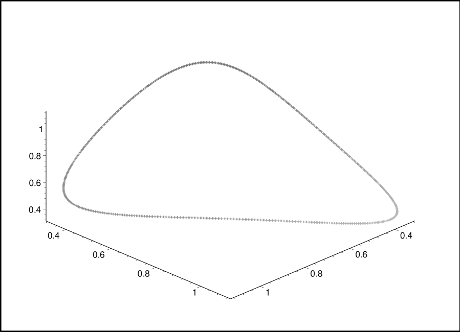
Figure 1: The orbit of the map (3.2) for $d=3$ with initial data $(v_{0},v_{1},v_{2})=\left(1,\frac{1}{2},\frac{2}{5}\right)$.

Appendix

6.1 Comment on the solution of the double pKdV equation

The double pKdV equation (1.3), which is equivalent to

$$\widehat{\widetilde{\widetilde{u}}}-\widehat{\widehat{\widetilde{u}}}-\left(\widehat{\widetilde{u}}-\widehat{\widehat{\widetilde{\widetilde{u}}}}\right)^{-1}=\widetilde{u}-\widehat{u}-\Big{(}u-\widehat{\widetilde{u}}\Big{)}^{-1},$$

is more general than the pKdV equation (1.1), that is

$$(u-\widehat{\widetilde{u}})(\widetilde{u}-\widehat{u})=1.$$

Here we explain how it is possible to obtain any solution of (1.3) from a solution of pKdV together with the solution of a linear equation.

To see this, let $a$ be a solution of the linear partial difference equation

$$\widehat{\widetilde{a}}=a.$$

(Note that, from (2.4), this is the same as the linear equation satisfied by the quantity J.) Then it can be verified by direct calculation that the combination

$$u=U+a$$

satisfies (1.3), where $U$ is any solution of (1.1). Conversely, let $u$ be any solution of (1.3), and define the quantity J in terms of $u$ according to the right hand formula in (2.4). Now let $a$ be a solution of the pair of linear equations

$$\widetilde{a}-\underset{\sim}{a}=\mathrm{J},\qquad\widehat{\widetilde{a}}=a.$$

It follows from (1.3) that the latter two equations are compatible, and the combination

$$U=u-a$$

satisfies the pKdV equation (1.1). Hence any solution of (1.3) can be written in the form $u=U+a$.

At the level of the $(d-1,-1)$-reduction of (1.3), this means that all solutions of the ordinary difference equation (2.7) can be written in the form

$$u_{n}=U_{n}+a_{n},$$

where $a_{n}$ is periodic with period $d$, as well as being a solution of the second order linear equation

$$a_{n+1}-a_{n-1}=J_{n},$$

and $U_{n}$ is a solution of the $(d-1,-1)$-reduction of (1.1) (as studied in reference [34]). It is not clear how this connection between the two reduced equations should be interpreted from the point of view of Liouville integrability.

6.2 An example of an orbit for $d=3$

Consider the choice of initial values $\tau_{0}=\tau_{1}=\tau_{2}=\tau_{3}=1$ for the Somos-4 recurrence with 2-periodic coefficients, as in Example 9, that is

$$\tau_{n+4}\,\tau_{n}=\alpha_{n}\,\tau_{n+3}\,\tau_{n+1}+\tau_{n+2}^{2},\qquad\mathrm{with}\qquad\alpha_{n+2}=\alpha_{n},$$

together with the choice of parameters $\alpha_{0}=1$, $\alpha_{1}=2$. This corresponds to taking the initial values $v_{0}=1$, $v_{1}=1/2$, $v_{2}=2/5$ in the map (3.2) with $d=3$, which is given by

$$\varphi:\quad(v_{0},v_{1},v_{2})\mapsto\left(v_{1},v_{2},\frac{v_{0}}{1+v_{2}v_{0}-v_{1}v_{0}}\right).$$

In Figure 1 we plot the orbit of the map $\varphi$ that is generated by this initial data.

References

- [1] V.E. Adler, A.I. Bobenko and Y.B. Suris. Classification of Integrable Equations on quad-graphs. The Consistency Approach. Commun. Math. Phys. 233 (2003) 513–43.
- [2] M. Błaszak. Multi-Hamiltonian Theory of Dynamical Systems. Springer, 1998.
- [3] M. Błaszak. From Bi-Hamiltonian Geometry to Separation of Variables: Stationary Harry-Dym and the KdV Dressing Chain. J. Nonlinear Math. Phys. 9, Supplement 1 (2002) 1–13.
- [4] M. Bruschi, O. Ragnisco, P.M. Santini and T. Gui-Zhang. Integrable symplectic maps. Physica D 49 (1991) 273–94.
- [5] H.W. Capel, F.W. Nijhoff and V.G. Papageorgiou. Complete integrability of Lagrangian mappings and lattices of KdV type. Phys. Lett. A 155 (1991) 377–87.
- [6] S. Fomin and A. Zelevinsky. Cluster algebras I: Foundations. J. Amer. Math. Soc. 15 (2002) 497–529.
- [7] S. Fomin and A. Zelevinsky. The Laurent phenomenon. Adv. in Appl. Math. 28 (2002) 119–144.
- [8] A.P. Fordy and R.J. Marsh. Cluster Mutation-Periodic Quivers and Associated Laurent Sequences. Journal of Algebraic Combinatorics 34 (2011) 19–66.
- [9] A.P. Fordy and A.N.W. Hone. Symplectic Maps from Cluster Algebras. SIGMA 7 (2011) 091.
- [10] A.P. Fordy and A.N.W. Hone. Discrete integrable systems and Poisson algebras from cluster maps. arXiv:1207.6072
- [11] D. Gale. The strange and surprising saga of the Somos sequences. Mathematical Intelligencer 13 (1) (1991) 40–42.
- [12] M. Gekhtman, M.Shapiro and A. Vainshtein. Cluster algebras and Weil-Petersson forms. Duke Math. J. 127 (2005) 291–311.
- [13] F.A. Haggar, G.B. Byrnes, G.R.W. Quispel and H.W. Capel. -integrals and -Lie symmetries in discrete dynamical systems. Physica A 233 (1996) 379–394.
- [14] R. Hirota. Nonlinear Partial Difference Equations. I. Difference Analogue of the Korteweg-de Vries Equation. Journal of the Physical Society of Japan 43 (1977) 1424–33.
- [15] P.H. van der Kamp. Initial value problems for lattice equations. J. Phys. A: Math. Theor. 42 (2009) 404019.
- [16] P.H. van der Kamp and G.R.W. Quispel. The staircase method: integrals for periodic reductions of integrable lattice equations. J. Phys. A: Math. Theor. 43 (2010) 465207.
- [17] P.H. van der Kamp, O. Rojas, and G.R.W. Quispel. Closed-form expressions for integrals of mKdV and sine-Gordon maps J. Phys. A: Math. Theor. 39 (2007) 12789.
- [18] I. Krichever, O. Lipan, P. Wiegmann and A. Zabrodin. Quantum Integrable Models and Discrete Classical Hirota Equations, Comm. Math. Phys. 188 (1997) 267–304.
- [19] S. Maeda. Completely Integrable Symplectic Mapping. Proc. Japan Acad. 63, Ser. A (1987) 198–200.
- [20] F. Magri. A simple model of an integrable Hamiltonian equation, J. Math. Phys. 19 (1978) 1156–1162.
- [21] A.V. Mikhailov (ed.). Integrability. Springer Lecture Notes in Physics 767, Springer-Verlag, Berlin, Heidelberg, 2009.
- [22] F.W. Nijhoff and H.W. Capel. The discrete Korteweg-de Vries equation. Acta Appl. Math. 39 (1995) 133–158.
- [23] F.W. Nijhoff. Discrete Systems and Integrability. Lect. Notes MATH3490, University of Leeds, 2006.
- [24] G.R.W. Quispel, F.W. Nijhoff, H.W. Capel and J. van der Linden. Linear integral equations and nonlinear difference-difference equations. Physica A 125 (1984) 344–380.
- [25] G.R.W. Quispel, J.A.G. Roberts and C.J. Thompson. Integrable mappings and soliton equations. Physics Letters A 126 (1988) 419–421.
- [26] G.R.W. Quispel, H.W. Capel, V.G. Papageorgiou and F.W. Nijhoff. Integrable mappings derived from soliton equations. Physica A 173 (1991) 243–66.
- [27] A. Ramani and B. Grammaticos. Discrete Painlevé equations: coalescences, limits and degeneracies. Physica A 228 (1996) 160–171.
- [28] J.A.G. Roberts. Understanding Non-QRT maps. Talk at Nonlinear Dynamical Systems, Melbourne, Australia, 28-30 September 2012.
- [29] R. Robinson. Periodicity of Somos sequences. Proc. Amer. Math. Soc. 116 (1992) 613–619.
- [30] M. Somos. Problem 1470. Crux Mathematicorum 15 (1989) 208.
- [31] Y.B. Suris. The Problem of Integrable Discretization: Hamiltonian Approach. Progress in Mathematics 219, Birkhauser Verlag, Basel, 2003.
- [32] D.T. Tran, P.H. van der Kamp, and G.R.W. Quispel. Closed-form expressions for integrals of traveling wave reductions of integrable lattice equations, J. Phys A.: Math. Theor. 42 (2009) 225201.
- [33] D.T. Tran. Complete integrability of maps obtained as reductions of integrable lattice equations. PhD thesis, La Trobe University, 2011.
- [34] D.T. Tran, P.H. van der Kamp and G.R.W. Quispel. Involutivity of integrals of sine-Gordon, modified KdV and potential KdV maps J. Phys. A: Math. Theor. 44 (2011) 295206.
- [35] A.P. Veselov. Integrable Maps. Russ. Math. Surveys 46 (1991) 1–51.
- [36] A.P. Veselov and A.B. Shabat. Dressing Chains and the Spectral Theory of the Schrödinger Operator. Func. Analysis Appl. 27 (1993) 81–96.
- [37] G.L. Wiersma and H.W. Capel. Lattice equations, hierarchies and Hamiltonian structures. Physica A 142 (1987) 199–244.
- [38] V.E. Zakharov (ed.). What is Integrability? Springer Series in Nonlinear Dynamics, Springer, 1991.