Structural Parameters of Galaxies in CANDELS

Abstract

We present global structural parameter measurements of 109,533 unique, $H_{\rm{F160W}}$-selected objects from the CANDELS multi-cycle treasury program. Sérsic model fits for these objects are produced with GALFIT in all available near-infrared filters ($H_{\rm{F160W}}$, $J_{\rm{F125W}}$ and, for a subset, $Y_{\rm{F105W}}$). The parameters of the best-fitting Sérsic models (total magnitude, half-light radius, Sérsic index, axis ratio, and position angle) are made public, along with newly constructed point spread functions for each field and filter. Random uncertainties in the measured parameters are estimated for each individual object based on a comparison between multiple, independent measurements of the same set of objects. To quantify systematic uncertainties we create a mosaic with simulated galaxy images with a realistic distribution of input parameters and then process and analyze the mosaic in an identical manner as the real data. We find that accurate and precise measurements – to 10% or better – of all structural parameters can typically be obtained for galaxies with $H_{\rm{F160W}}<23$, with comparable fidelity for basic size and shape measurements for galaxies to $H_{\rm{F160W}}\sim 24.5$.

1. Introduction

The Cosmic Assembly Near-Infrared Deep Extragalactic Legacy Survey (CANDELS) constitutes 902 orbits of Hubble Space Telescope (HST) observing time. One of the primary motivations for CANDELS is the investigation of galaxies at redshifts $z\sim 1.5-3$, and in particular their structural and morphological properties (Grogin et al., 2011). This paper describes the characterization of structural galaxy properties in the HST WFC3/IR imaging mosaics (Koekemoer et al., 2011) through fitting the observed surface brightness distributions by two-dimensional parametrized models, whose surface brightness profiles follow the Sérsic law (Sérsic, 1968). The resulting catalogs are made public online.

Over the previous decade WFPC2 and ACS have enabled comprehensive structural and morphological studies of the galaxy population up to $z\sim 1$ at ‘optical’ wavelengths (e.g., Giavalisco et al., 2004; Rix et al., 2004; Scoville et al., 2007). At redshifts $z>1$ WFPC2 and ACS observations sample the rest-frame ultra-violet, which complicates the interpretation of galaxy images, as dust can strongly attenuate the light and young stars that contribute little to the underlying stellar mass distribution dominate over the older population.

For about a decade now, deep near-infrared surveys have been conducted to remedy this (e.g., Labbé et al., 2003; Fontana et al., 2004; Quadri et al., 2007; Lawrence et al., 2007; Capak et al., 2007). These ground-based surveys have provided large samples, and despite the limited spatial resolution (typically 0.4-0.8″, or $\sim 3-6$ kpc at $z>1$), general and fundamental structural properties have been measured out to $z\sim 2$ (Trujillo et al., 2004, 2006; Franx et al., 2008; Williams et al., 2009; Chang et al., 2012). Galaxies were shown to be smaller in the past, and at all redshifts their sizes were found to correlate with star-formation activity. As in the local universe, galaxies with low star-formation activity tend to be smaller than galaxies with high (or normal) star-formation rates.

The use of ground-based near-infrared imaging for the purpose of investigating the internal structure of galaxies and its evolution has largely been limited to simple size measurements. Any examination of galaxy structure beyond this requires HST resolution. Near-infrared observations with NICMOS over relatively small areas and targeted sampling of small numbers of pre-selected galaxies have before revealed some fundamental aspects of structural properties at $z\sim 2$. Beyond confirming the size evolution of galaxies, the profoundly different structure of high-$z$ galaxies could now be fully appreciated. The discovery of massive, yet very small, galaxies (Zirm, 2007; Toft et al., 2007) posed a surprise to the community, and has instigated much debate regarding the formation and evolution of the most massive galaxies. Moreover, the concentration of $z\sim 2$ galaxy light profiles, presumably tracing the bulge-to-disk ratio, was found to correlate with star-formation activity, indicating that galaxies with low star-formation rates have larger bulges at all $z\lesssim 2$ (e.g., Kriek et al., 2009).

The arrival of WFC3 has now allowed the exploration of galaxy structure at $z>1$ with unprecedented data quality and sample sizes. The Ultra Deep Field (UDF) program (Bouwens et al., 2010) broke ground in terms of depth and resolution, confirming previous claims on the structural properties of $z\sim 2$ galaxies and revealing further detail on their morphology and structure (e.g., Szomoru et al., 2010). Results from the HST/WFC3 Early Release Science (ERS) program (Windhorst et al., 2011) foreshadowed the power of CANDELS. That modestly sized ERS program provided data quality and quantity on par with the largest NICMOS data sets in existence (Scoville et al., 2007; Conselice et al., 2011) and produced new insights into the basic structural parameters (e.g., van der Wel et al., 2011; Cassata et al., 2011) and morphologies (e.g., Cameron et al., 2011) of $z\sim 2$ galaxies.

CANDELS fills the gap between the ground-based surveys and the existing HST near-infrared surveys. It provides much larger samples than previous near-infrared HST data sets and much improved depth and resolution compared to ground-based surveys. Wuyts et al. (2011) and Bell et al. (2012) showed with unprecedented clarity how star-formation activity and structure are strongly related. Papovich et al. (2012) and Lotz et al. (2011) examined the environmental dependence of galaxy sizes and merger frequency, respectively. Moreover, the larger area allows to study the properties of more rare objects. Kocevski et al. (2012) compared the morphologies of galaxies that do and do not host AGN and concluded there is no significant difference, and Kartaltepe et al. (2011) found a tentative connection between extreme star formation activity and merging.

CANDELS also allows us to probe galaxy structure down to previously unattainable low mass and luminosity limits – apart from the UDF – in particular through the deep segment of the survey. Furthermore, the structure of massive galaxies beyond $z=3$, where knowledge is still sparse, can be explored (e.g., Caputi et al., 2012; Guo et al., 2012). Finally, CANDELS aims at obtaining for the first time a comprehensive view of the morphologies of $z>4$ Lyman-break and Ly-$\alpha$ emitters at wavelengths longer than $2000\AA$ in the rest frame.

In this paper we describe the measurements of structural parameters of 109,533 unique objects in the CANDELS WFC3/IR data, representing roughly 2/3 of the full survey. Our online materials will be updated with the final 1/3 of the survey once observations have been completed by the end of 2013. We describe the imaging, object detection, and background flux level estimation in §2. In §3 we construct Point Spread Function (PSF) models that are used as the default PSFs in the CANDELS collaboration; these models are also made public. Using GALAPAGOS (Barden et al., 2012) we prepare flux and noise image cutouts and describe how GALFIT (Peng et al., 2010) is used to produce single-component Sérsic model fits (§4). We estimate random and systematic uncertainties in the parameter estimates through the comparison between different image data sets of the same objects, and Sérsic fits to simulated galaxy images (§5). We provide in §6 a description of the content of all published materials.

Table 1 Publication dates of CANDELS catalogs with GALFIT -based structural parameters published online. Those in bold face are published along with this paper. The rest will be published over the next year, within 4 months after the last observation of each field.

Field	F105W	F125W	F160W
COSMOS	$\cdots$	12/2012	12/2012
EGS	$\cdots$	09/2013	09/2013
GOODS-N	12/2013	12/2013	12/2013
GOODS-S	12/2012	12/2012	12/2012
UDS	$\cdots$	12/2012	12/2012

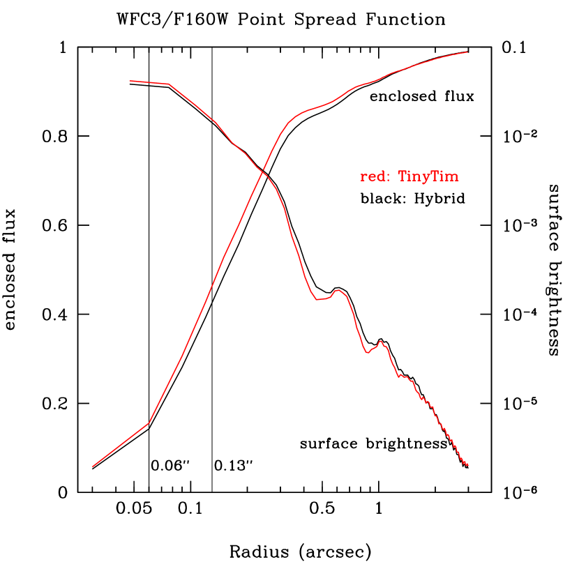
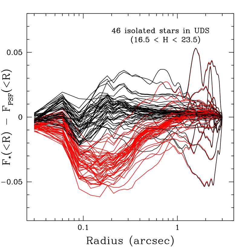
Figure 1.— Left: Comparison between two HST/WFC3 F160W model PSFs. In red we show the TinyTim model PSF, in black a hybrid of a stacked star (outside a radius of 3 drizzled pixels, i.e. , 0.18″) and the TinyTim model (inside that radius). The two sets of curves show the enclosed flux (left-hand y-axis) within the radius $r$ shown on the x-axis, and the surface brightness per pixel (right-hand axis) at radius $r$. The vertical lines indicate the original WFC3 pixel scale ($0.13\arcsec$) and the drizzled pixel scale of the mosaics used for the profile fitting in the paper ($0.06\arcsec$). The growth curves are normalized to the total flux of the model PSF within $10\arcsec$ and the growth curves of the empirical PSFs is forced to coincide with the that of the model PSF at $3\arcsec$. The surface brightness curves are azimuthally averaged and in units of fractional PSF flux per $0.06\arcsec$ pixel. Right: The residuals from individual stars after subtracting the TinyTim model PSF (red) and the hybrid model PSF (black). The systematic negative trend for the TinyTim model indicates that a larger fraction of the flux of a star resides at radii $0.2-1$″than what the TinyTim model predicts. Our hybrid model PSF does not show such a trend and follows the light profiles of the isolated stars out to radii of 3″.

2. HST/WFC3 Imaging Mosaics

2.1. Fields and Filters

A full description of the CANDELS observing program is given by Grogin et al. (2011) and Koekemoer et al. (2011). CANDELS is a WFC3 and parallel ACS, 902 orbit HST imaging survey; here we concentrate on the WFC3 data only, which covers 800 arcmin² and is distributed over five widely separated fields. There is a ‘deep’ and a ‘wide’ component. About 125 arcmin², divided over two fields, will have $\sim$13 orbits per tile divided over three filters (F105W, F125W, and F160W), and the remaining area, distributed over five fields, will have $2-3$ orbits per tile divided over two filters (F125W and F160W). These exposures reach $H_{\rm{F160W}}\sim$28 and $H_{\rm{F160W}}\sim$27 5$\sigma$ magnitude limits for point sources in each filter for the ‘deep’ and ‘wide’ imaging, respectively.

Along with this paper we electronically release structural parameter catalogs for the three fields for which observations have been completed at the time of writing, as summarized in Table 1, namely, the Ultra Deep Survey field (UDS, Lawrence et al., 2007), the Cosmological Evolution Survey field (COSMOS, Scoville et al., 2007) (both 9$\arcmin\times 24\arcmin$ arcmin and each at ‘wide’ depth), and the Great Observatories Origins Deep Survey-South field (GOODS-S, Giavalisco et al., 2004): ‘wide’ over 4$\arcmin\times 10\arcmin$; ‘deep’ over 7$\arcmin\times 10\arcmin$. Note that these dimensions refer to the CANDELS coverage, not to the dimensions of the data sets that define the original surveys.

The CANDELS observations are augmented by previously obtained WFC3/IR data from the Early Release Science program (ERS, Windhorst et al., 2011) in the Northern part of the GOODS-S field (4$\arcmin\times 9\arcmin$ at 2-orbit depth in F098M, F125W, and F160W) and the Ultra Deep Field (UDF) program (Bouwens et al., 2010) embedded in the GOODS-S deep area (1 pointing with $\sim$15 orbits in F105W and F125W, and 28 orbits in F160W). The electronically available catalogs published along with this paper, derived from the finalized CANDELS imaging products at the date of publication, will be updated upon completion of the two remaining fields: GOODS-North and the Extended Groth Strip (EGS, Davis et al., 2007). Image, weight (inverse variance), and exposure time mosaics are prepared by drizzling the individual exposures onto a grid with rescaled pixel sizes of 0.06$"$. This procedure is described in detail by Koekemoer et al. (2011).

2.2. Object Identification

We use a modified version of SExtractor (Bertin & Arnouts, 1996) v2.5 to identify objects in the CANDELS F160W mosaics. We refer to Galametz et al. (in prep.) for a full description of the source extraction but the main steps are as follows. The first modification to SExtractor is that we added a buffer between the isophotal area of each object and pixels used to estimate the local background. Note that this modification affects object identification and segmentation map construction, but the newly measured background is not used in the surface brightness profile fits (see below). The second modification is the removal of a bug that previously allowed disconnected regions to have the same value in the segmentation map, and therefore have the same identification number. Our modified version produces objects consisting of adjacent pixels only.

SExtractor is run in dual mode, using the F160W mosaics both as the detection images and the measurement images. Indeed we found slight differences with respect to single-mode SExtractor output, which we wish to avoid in order to allow direct comparisons with dual-mode photometry of objects detected in F160W and measured in other filters.

Catalogs for two sets of SExtractor detection parameters, the ‘cold’ setup and the ‘hot’ setup are produced separately and then combined in an approach introduced by Barden et al. (2012). The ‘cold’ setup focuses on optimal segmentation of relatively bright objects. This avoids that star-forming galaxies are spuriously split up into multiple components by deblending too aggressively. The ‘cold’ setup selects objects with 0.75$\sigma$ detections over 5 adjacent pixels after smoothing with a top-hat kernel with a diameter of 9 pixels. Objects are deblended adopting 9 logarithmic sub-thresholds relative to the maximum count value of an object and using a minimum contrast of 0.0001. Given that the PSF has a FWHM much smaller than that of the smoothing kernel used in the ‘cold’ setup, this approach is suboptimal for detecting small, faint objects.

This is mitigated by the ‘hot’ setup, which uses a Gaussian smoothing kernel with a FWHM of 4 pixels that is similar to that of the PSF and selects objects with 10 adjacent pixels with 0.7$\sigma$ fluxes. Deblending is done with the default SExtractor parameters: a minimum contrast of 0.001 and 64 logarithmic sub-thresholds.

Each object in the ‘hot’ catalog that falls within an aperture around an object in the ‘cold’ catalog is considered part of the latter and removed from the combined catalog. This elliptical aperture is 2.5 times the elliptical Kron radius as measured with the default SExtractor parameters. The size and shape of the ellipse are calculated from the second-order moment of the flux distribution. In the combined segmentation map the segmented pixels of the removed ‘hot’ object are added to the object in the ’cold’ segmentation map.

In total, we identify 109,533 unique objects in the F160W mosaics. HST resolution enables us to resolve close companions, which is essential when one is interested in the measurement of the structures of individual galaxies. 7% (9%) of objects in CANDELS ‘wide’ (‘deep’) have one or more neighbors within 1$\arcsec$; they would typically not be resolved in ground-based imaging data sets.

The SExtractor measurements of object magnitudes, size, shape and orientation are used to provide GALFIT with initial guesses for the fitting parameters (see §4.2). This helps in terms of computing time and ensures that GALFIT converges to the global $\chi^{2}$ minimum in parameter space.

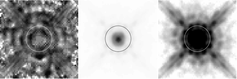
Figure 2.— Left: Ratio of our hybrid PSF and the TinyTim model, both for the UDS field, with dark regions lower levels in the TinyTim model (the darkest regions have values $>2$). The image is 3.6″$\times$3.6″, and the circle, which has been included to guide the eye, has a radius of 0.6″. The area near the center has a constant value by construction as we use the TinyTim model in our hybrid for the central pixels. We show our hybrid PSF with two different stretches in order to to emphasize the bright, central region (Middle) and the faint, outer region (Right). At each radius, the brightest parts of the PSF are reproduced quite accurately by the TinyTim model; rather, it is in between the diffraction spikes and Airy rings that the deviations are largest, and at a level that cannot be explained by noise. These features cause the systematic differences between the light profiles of stars and the TinyTim model shown in Figure 1.

2.3. Background Estimation

The image cutouts we use for model fitting (§4.1) are too small for GALFIT to optimally determine the background flux level. In order for the image to be large enough for an accurate, simmulataneous determination of both the structural parameters and the background flux level, the number of objects that would have to be fit simultaneously would become impractical, if not impossible in some cases (at present, GALFIT cannot fit more than 110 objects at one time).

The pipeline GALAPAGOS  (Barden et al., 2012) remedies this problem. Originally written to analyze ACS mosaics from GEMS (Rix et al., 2004), GALAPAGOS determines the background from the full mosaic and then runs GALFIT using this background value along with initial guesses for the input parameters based on the SExtractor output described above.

The independent background estimate is the main feature of GALAPAGOS that elevates it beyond the level of ‘just’ a smart wrapper for SExtractor and GALFIT . In short, ignoring pixels within a certain distance of an object, the flux is computed in a series of annuli, searching for a converging flux level at sufficiently large distances from the target object. This background flux level is provided to GALFIT , which keeps it fixed at that value. In §5.1 we investigate the contribution of the uncertainty in the background to the uncertainties in the structural parameters.

3. Point Spread Function

Besides an accurate noise model and background estimation, good knowledge of the PSF is essential for the accuracy of the parameter estimation. This necessitates the production of custom-made PSF models for each of the mosaics and each of the filters. These PSF models should be used for all PSF-dependent analyses of the public CANDELS imaging mosaics, and are therefore released here (see §6 for a summary of the published material).

The PSF has a FWHM of $\sim$0.17″ for the F160W filter. Individual exposures (typically 800s) are dithered to improve on the originally coarse sampling – the pixel scale of the WFC3/IR camera is 0.13″. Using the TinyTim package (Krist, 1995) we construct a model PSF for the respective imaging mosaics for the different fields and filters. Briefly, TinyTim PSF models are created for the center of the WFC3 detector assuming a G2V spectral type. The PSFs are sub-sampled by a factor of ten in order to aid in aligning them with the CANDELS dither pattern. They are then re-sampled to the WFC3 pixel scale and a kernel is applied to replicate the effects of inter-pixel capacitance (Hilbert & McCullough, 2011). Finally, PSFs at each dither position are distortion-corrected and combined with the same drizzle parameters used in producing the imaging mosaics (Koekemoer et al., 2011).

As an example we show the growth curve and surface brightness profile of the F160W PSF for the UDS (Figure 1 – red lines in the left-hand panel). To verify the accuracy of this model PSF we subtract it from a sample of 46 isolated stars in the F160W UDS mosaic (after normalizing the star fluxes within a radius of 3″, and examine the residual enclosed flux (Figure 1 – red lines in the right-hand panel). The systematic residual of $\sim-4$% seen at $\sim$0.2″ implies that the model PSF contains $\sim$4% less light outside an aperture $\sim 0.2$″ than point sources in the actual data. Background levels, computed as described in §2.3, are low compared to the stellar fluxes, even at radii of $1-3$″, such that the enclosed flux is affected by less than 1% at any radius. In other words, background errors cannot explain the large differences between stellar and model PSF growth curves at relatively small radii. Such an erroneous PSF model, which is seen for other fields and filters as well, can affect the measurement of structural parameters of small, concentrated objects at a level that exceeds the formal, random uncertainty.

The difference between the stars and the TinyTim model occurs in relatively ‘dark’ areas seen in Figure 2. The center, the diffraction spikes, and the dot-like features associated with the first Airy ring are well reproduced by TinyTim , whereas regions in between those features are too dark. The origin of this feature remains unexplained.

We use the 46 isolated stars shown in the right-hand panel of Figure 1 in median-stacked form as an alternative PSF representation. The problem with this approach is the variety in the sub-pixel positioning of the stellar images, which leads to broadening in the PSF model when stacking a number of stars.

In order to provide an accurate PSF model at all radii we take the median-stacked star and replace the central pixels (within a radius of 3 pixels from the center) by the TinyTim model PSF. The flux values of these pixels are normalized such that the total flux of the newly constructed hybrid PSF model is the same as that of the stacked star. The accuracy of the model PSF in the central region is confirmed by its good correspondence with the flux distributions of the small number stars that happen to be well-aligned with the brightest pixel. Note that there are too few such stars to produce a stacked PSF with sufficient signal-to-noise ratio at larger radii.

The growth curves, surface brightness profiles and residuals are shown in black in Figure 1. The residuals show much smaller systematic effects than the best-effort TinyTim model PSF, indicating that the hybrid PSF provides a good description of the growth curves of individual stars out to 3″.

We construct equivalent hybrid PSF models for all fields and filters. For the UDS and COSMOS fields we created PSF models for the F125W and F160W PSF filters. For GOODS-S the situation is more complex. For the ERS region we have F098M, F125W and F160W PSF models; for the ‘wide’ and ‘deep’ regions we created separate F105W, F125W and F160W PSF models; for the UDF, which is very small and contains few stars, we simply make use of a single star. Replacing the central pixels by model values does not work well for a single star, but the chosen star is bright and isolated, and happens to be be relatively well-centered on the brightest pixel, and thus serves its purpose well.

The fact that variations are $\lesssim 2$% for all stars implies that PSF differences due to variations in position, color, and magnitude are negligible for our GALFIT measurements. We note that small variations in dither pattern, orientation and general mosaic geometry exist within the distinct fields. This implies that some fraction of the objects will not have precisely the correct PSF model. This is unavoidable when using stars to produce the PSF model.

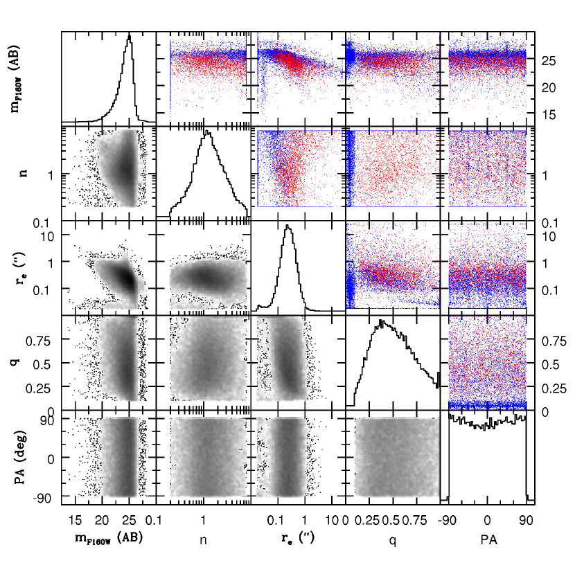
Figure 3.— The distribution of the GALFIT -derived parameters F160W magnitude, Sérsic index, effective radius, axis ratio, and position angle for objects in the three CANDELS fields analyzed here (COSMOS, GOODS-South, and UDS). The panels with gray scale distributions represent the objects with flag value zero (these are objects with good fits – see §4.3). On the diagonal we show for the flag zero sample the histogram of each of the five parameters in units as shown on the x-axis. The typical galaxy has magnitude $H_{\rm{F160W}}\sim 25$, $n\sim 1$, $r_{e}\sim 0.3\arcsec$, and $q\sim 0.4$. The colored panels show the distribution of objects with flag value one (red) and flag value two (blue) – these are objects with, respectively, suspicious and bad fits as explained in §4.3.

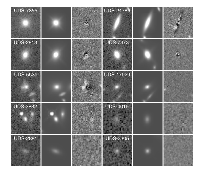
Figure 4.— Ten galaxy images (left) from the UDS F160W mosaic and their GALFIT models (middle) and residuals (right). These objects have been chosen to have a range in magnitude (increasing from $H_{\rm{F160W}}\sim 20$ at the top left to $H_{\rm{F160W}}\sim 25$ at the bottom right) and structure. UDS-7335 and UDS-2813 have $n\sim 4$ and smooth light profiles characteristic of early-type galaxies; UDS-24786 and UDS-7373 have $n\sim 1$ and show more substructure, characteristic of star-forming, late-type galaxies. For the faintest galaxies shown here the GALFIT model still captures the basic structural parameters such as size and shape. In several cases multiple objects are fit simultaneously, illustrating the procedure described in §4.2.

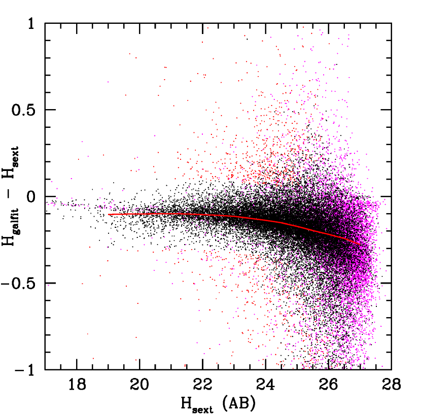
Figure 5.— Comparison of GALFIT and SExtractor (BEST) F160W magnitudes for objects in the UDS. The y-axis shows the difference between the two. Black points represent objects that we have assigned flag value 0 (good fits); red points have flag value 1 (suspect fits); magenta points have flag value 2 (bad fits – bright stars have bad fits because they are point sources). See §4.3 for a full explanation of the flag definitions. The red line is a running median for the black and red points, quantifying the systematic offset between GALFIT and SExtractor total magnitudes. Note that these systematic offsets are in excess of the random uncertainty in the GALFIT -based total magnitudes.

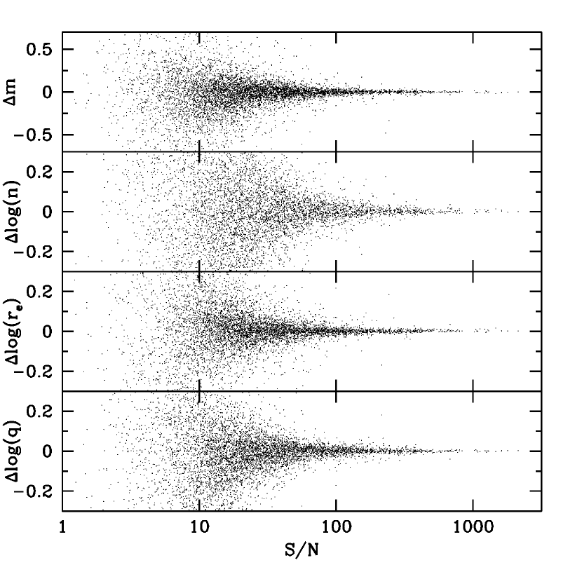
Figure 6.— Difference between the structural parameter estimates from deep and shallow images of 6492 objects in GOODS-S as a function of $S/N$ in the shallow up. The spread reflects the uncertainty in the measurements, which we use in §5.1 to assign uncertainties to the structural parameter measurements of all galaxies. Although dependencies on other parameters exist (see Figures 7 and 8), the uncertainty depends to first order on $S/N$.

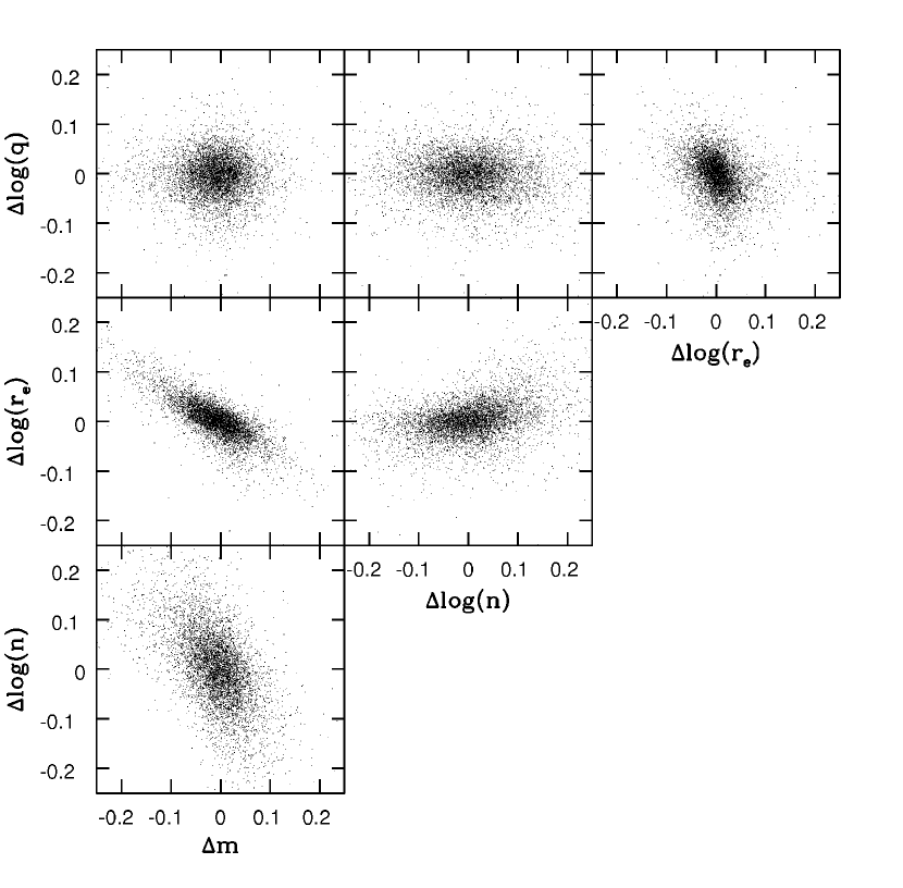
Figure 7.— Correlations among structural parameter measurement uncertainties (also see, e.g., Häussler et al., 2007; Guo et al., 2009; Bruce et al., 2012). All quantities $\Delta$ are the difference between the structural parameters are measured from the deep and shallow images of 6492 galaxies. $\Delta$ is normalized to $S/N=50$ as described in the text; that is, first-order effects on $S/N$ are removed. Particularly relevant are the strong correlations between the uncertainties in magnitude ($m$), Sérsic index ($n)$ and effective radius ($r$): uncertainties in $m$ and $r$ correlate such that any overestimate (underestimate) in $r$ corresponds linearly with an overestimate (underestimate) in the total flux; analogously, if the total flux is overestimated (underestimated) by 5%, the Sérsic index is typically overestimated (underestimated) by as much as 25%. The shape and amplitude of these ‘error ellipses’ (or rather, ‘ellipsoids’, as they are at least 3-dimensional) depend on the parameters themselves and therefore do not represent the covariance matrix of the uncertainties for the sample as a whole.

4. Modeling Light Profiles

4.1. Preparation of Image and Noise Cutouts

For each of the 109,533 objects, an image cutout, in units of electrons per second, is produced from the large mosaic. The size of each rectangular cutout is determined by the Kron radius, ellipticity and position angle as measured by SExtractor , and is chosen to enclose an ellipse with major axis length 2.5 times the Kron ellipse ($A_{IMAGE}\times KRON_{RADIUS}$ in SExtractor parlance). This typically corresponds to $\sim 30$ times the half-light radius of an object.

A noise map of the same size is also produced. The pixel values in the noise map have units of electrons per second, and are the square root of the total variance. The total variance is estimated by starting with the computed variance, referred to by Koekemoer et al. (2011) as the ‘intrinsic’ term (e.g., background noise and readout noise), in units of electrons. We add the variance at each pixel from the Poisson noise due to the objects themselves. We divide by the (computed) exposure time for each pixel to make the units consistent with those of the images.

The images and noise maps are used by GALFIT as inpu. We note that GALFIT does not have all necessary information about the image characteristics required for a self-contained noise-estimate as a result of the extensive process from raw, single exposures, to final, drizzled mosaics. Therefore, especially for bright, compact objects it is essential to use the noise maps we construct rather than the GALFIT ’s own noise estimation. In practice, for objects brighter than $H_{\rm{F160W}}\sim 22-23$ – corresponding to the typical background WFC3/F160W flux level measured over an area the size of a typical object – the extrinsic noise term begins to dominate.

We compute signal-to-noise ratio ($S/N$) for each object from their images and noise maps, integrating over the pixels that belong to the objects according to the segmentation map. An object with $H_{\rm{F160W}}\sim 22$ has $S/N\sim 100-200$ for the ‘wide’ data. These $S/N$ estimates are used in our derivation of the measurement uncertainties in §5.

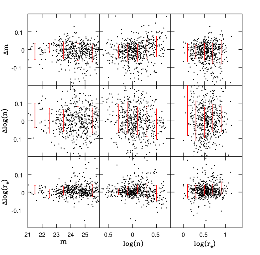
Figure 8.— Correlation between structural parameter measurement uncertainties and measured structural parameters. On the x-axis three parameters (magnitude, $m$, Sérsic index, $n$, and effective radius, $r$) as measured from the GSD deep region are shown. The galaxies displayed in the first column of panels (showing $m$), are chosen within narrow ranges of $n$ and $r$ around the median values in the full catalog. In the second (third) column the same is done for $n$ ($r$): $m$ and $r$ ($n$) are chosen within a narrow range. On the y-axis the difference $\Delta$ between the measurements from the deep and shallow images of the same objects are shown: the scatter in $\Delta$ reflects the uncertainty, indicated in red by the running 16-84%-tile ranges. As in Figure 7, all $\Delta$ are normalized to $S/N=50$. Strong second-order effects remain, most clearly seen in the dependence of the uncertainty in $r$ and $m$ on $n$ and the dependence of the uncertainty in $n$ and $m$ on $r$.

4.2. GALFIT Setup

The image cutouts, along with the noise model, the appropriate PSF model, and the pre-determined, fixed background level, are provided to GALFIT , which is used to find the best-fitting Sérsic model for each object. The fitting parameters are total magnitude ($m$), half-light radius ($r$) measured along the major axis, Sérsic index ($n$), axis ratio ($q$), position angle ($PA$), and central position. Initial guesses for these parameters are taken from the SExtractor detection catalog. A constraints file is constructed so that GALFIT is forced to keep the Sérsic index between 0.2 and 8, the effective radius between 0.3 and 400 pixels, the axis ratio between 0.0001 and 1, the magnitude between 0 and 40, and, between -3 and +3 magnitudes from the input value (the SExtractor magnitude).

Neighboring objects in each image cutout are fit simultaneously or masked out, depending on their brightness compared to the main target: galaxies are fit simultaneously if they are less than 4 magnitudes fainter than the main target; stars are fit simultaneously if they are less than 2 magnitudes fainter. In order to produce a good model, it is sometimes necessary to also fit objects outside the image cutout. The decision to do so depends on the contribution of objects outside the image cutout to the flux in the cutout. SExtractor or previously obtained GALFIT measurements are used to make informed decisions. The entire decision process, carried out by GALAPAGOS , is quite sophisticated and we refer to Barden et al. (2012) for a full description. Note that the segmentation maps described in §2.2 are only used to identify objects, and not to identify the pixels that are used in the Sérsic  fits.

For illustrative purposes, the images of 10 galaxies and their fits are shown in Figure 4. All best-fitting GALFIT parameters are listed in Table 2 and shown in Figure 3. The typical galaxy with a good Sérsic model fit (see §4.3 for the definition of ‘good’) has magnitude $H_{\rm{F160W}}\sim 25$, Sérsic index $n\sim 1$, effective radius $r_{e}\sim 0.3\arcsec$, and axis ratio $q\sim 0.4$. The position angle distribution is not entirely uniform; this is due to unresolved sources, mostly stars. For resolved sources the distribution is uniform.

Table 2 GALFIT fitting results and derived uncertainties. This table gives a sample of the UDS F160W catalog. Electronic versions of the full catalogs for all fields and (near-infrared) filters, as listed in Table 1, are published online (see §6. $m$ is the AB magnitude, $r$ is the half-light semi-major axis in arcseconds, $n$ is the Sérsic index, $q$ is the projected axis ratio, $PA$ is the position angle in degrees ($PA=0$ corresponds to North; $PA=90$ corresponds to East). $S/N$ is the signal-to-noise ratio measured over the pixels in the segmentation map that are attributed to the object. The listed uncertainties are based on population statistics and derived as described in §5.1 and correspond to the half-width of the 68%-confidence interval (i.e., these are 1$\sigma$ error bars in the case of gaussianity).

ID	RA	DEC	FLAG	$m\pm\delta m$	$r\pm\delta r$	$n\pm\delta n$	$q\pm\delta q$	$PA\pm\delta PA$	$S/N$
	J2000	J2000		AB mag	$\arcsec$			$\deg$
1	34.223766	-5.278053	3	-999 $\pm$ -999	-999 $\pm$ -999	-999 $\pm$ -999	-999 $\pm$ -999	-999 $\pm$ -999	5.43
2	34.223904	-5.277949	0	24.41 $\pm$ 0.40	0.43 $\pm$ 0.20	0.80 $\pm$ 1.03	0.18 $\pm$ 0.09	41.61 $\pm$ 14.32	6.88
3	34.223492	-5.277952	0	25.17 $\pm$ 0.24	0.18 $\pm$ 0.06	0.27 $\pm$ 0.28	0.74 $\pm$ 0.37	-52.04 $\pm$ 23.24	8.57
4	34.265106	-5.277749	1	23.06 $\pm$ 0.19	0.27 $\pm$ 0.07	1.49 $\pm$ 0.84	0.72 $\pm$ 0.19	67.92 $\pm$ 10.47	13.33
5	34.295372	-5.277648	1	21.06 $\pm$ 0.09	1.16 $\pm$ 0.11	1.55 $\pm$ 0.28	0.80 $\pm$ 0.08	-62.85 $\pm$ 3.57	33.46
.	.	.	.	.	.	.	.	.	.
.	.	.	.	.	.	.	.	.	.
.	.	.	.	.	.	.	.	.	.

Table 3 Systematic and random uncertainties in structural parameters for CANDELS ‘wide’ imaging in F160W. The systematic uncertainties are derived from GALAPAGOS processing of simulated images as described (see §5.2); the random uncertainties are inferred from GALAPAGOS processing of different data sets of the same galaxies as described in §5.1 . The systematic uncertainties are given first, followed by random uncertainties as error bars. For $m$ the units are in magnitudes; for the other parameters the uncertainties are relative, in linear units (they correspond to percentages). The galaxy samples are split by Sérsic index (at $n=3$) and effective radius (at $r_{e}=0.3"$).

	$\Delta m$				$\Delta n$
$m$	$n<3$	$n>3$	$r_{e}<0.3"$	$r_{e}>0.3"$	$n<3$	$n>3$	$r_{e}<0.3"$	$r_{e}>0.3"$
21	$-0.02\pm 0.01$	$-0.01\pm 0.01$	$-0.02\pm 0.01$	$-0.01\pm 0.01$	$-0.01\pm 0.02$	$-0.03\pm 0.03$	$-0.02\pm 0.02$	$-0.00\pm 0.02$
22	$-0.01\pm 0.02$	$0.00\pm 0.02$	$-0.01\pm 0.01$	$-0.01\pm 0.02$	$-0.03\pm 0.04$	$-0.06\pm 0.06$	$-0.05\pm 0.04$	$-0.01\pm 0.05$
23	$-0.01\pm 0.03$	$0.06\pm 0.07$	$-0.01\pm 0.03$	$0.01\pm 0.05$	$-0.01\pm 0.10$	$-0.09\pm 0.16$	$-0.01\pm 0.09$	$-0.03\pm 0.13$
24	$-0.01\pm 0.06$	$0.13\pm 0.13$	$-0.01\pm 0.05$	$0.05\pm 0.12$	$-0.01\pm 0.24$	$-0.25\pm 0.33$	$-0.01\pm 0.23$	$-0.11\pm 0.33$
25	$-0.04\pm 0.13$	$0.10\pm 0.21$	$-0.03\pm 0.12$	$0.03\pm 0.25$	$0.02\pm 0.49$	$-0.49\pm 0.58$	$0.00\pm 0.45$	$-0.20\pm 0.68$
26	$-0.14\pm 0.26$	$0.02\pm 0.31$	$-0.13\pm 0.25$	$-0.09\pm 0.44$	$0.31\pm 0.86$	$-0.84\pm 0.92$	$0.23\pm 0.84$	$-0.16\pm 1.21$
27	$-0.47\pm 0.41$	$-0.37\pm 0.54$	$-0.46\pm 0.42$	$\cdots$	$0.99\pm 1.28$	$-1.59\pm 1.46$	$0.87\pm 1.29$	$\cdots$
	$\Delta r_{e}$				$\Delta q$
$m$	$n<3$	$n>3$	$r_{e}<0.3"$	$r_{e}>0.3"$	$n<3$	$n>3$	$r_{e}<0.3"$	$r_{e}>0.3"$
21	$0.00\pm 0.01$	$0.00\pm 0.016$	$0.01\pm 0.01$	$0.00\pm 0.01$	$0.01\pm 0.01$	$-0.01\pm 0.02$	$0.01\pm 0.01$	$0.0\pm 0.01$
22	$0.01\pm 0.02$	$-0.02\pm 0.04$	$0.02\pm 0.02$	$-0.01\pm 0.02$	$0.00\pm 0.02$	$0.01\pm 0.03$	$0.00\pm 0.02$	$0.0\pm 0.03$
23	$0.00\pm 0.04$	$-0.10\pm 0.11$	$0.00\pm 0.03$	$-0.03\pm 0.06$	$0.00\pm 0.05$	$-0.01\pm 0.08$	$0.00\pm 0.04$	$0.00\pm 0.06$
24	$0.01\pm 0.08$	$-0.22\pm 0.19$	$0.01\pm 0.08$	$-0.10\pm 0.15$	$-0.02\pm 0.11$	$-0.03\pm 0.18$	$-0.02\pm 0.10$	$-0.02\pm 0.15$
25	$0.04\pm 0.19$	$-0.19\pm 0.33$	$0.04\pm 0.18$	$-0.09\pm 0.33$	$-0.07\pm 0.25$	$-0.07\pm 0.35$	$-0.07\pm 0.24$	$-0.04\pm 0.35$
26	$0.12\pm 0.43$	$-0.11\pm 0.55$	$0.12\pm 0.42$	$-0.11\pm 0.63$	$-0.17\pm 0.51$	$-0.09\pm 0.59$	$-0.17\pm 0.51$	$0.06\pm 0.69$
27	$0.27\pm 0.75$	$0.22\pm 0.85$	$0.27\pm 0.76$	$\cdots$	$-0.28\pm 0.81$	$0.40\pm 0.90$	$-0.25\pm 0.82$	$\cdots$

4.3. Flags

In Table 2 we flag objects with suspicious (flag value 1), bad (2), or non-existent (3) fitting results. All other objects (good fits) have flag value of zero. Suspicious fitting results (with flag value 1) are those where the GALFIT magnitude deviates from the expected magnitude by more than three times the uncertainty in the GALFIT magnitude derived as described below, in §5.1. This comparison is illustrated in Figure 5, where we show the GALFIT and SExtractor magnitudes for the UDS F160W measurements. The expected magnitude is the BEST magnitude from SExtractor , corrected for the systematic, magnitude-dependent offset between GALFIT model magnitude and the BEST magnitude, indicated by the red line in the figure. The BEST magnitude is measured in $H_{\rm{F160W}}$, adding the color, e.g., $J_{\rm{F125W}}-H_{\rm{F160W}}$, measured over the $H_{\rm{F160W}}$ segmentation map. This offset between the SExtractor and GALFIT magnitudes is 0.1 mag for bright sources and increases to 0.3 mag for faint sources (see Figure 5). This offset has been noted by many authors before (e.g., Holden et al., 2005; Blakeslee et al., 2006; Häussler et al., 2007). The distribution of GALFIT fitting parameters with flag value 1 is shown in red in Figure 3.

Objects with flag value 1 are not necessarily bad fits and in some cases can be used without problem. However, we recommend to assess on an object-by-object basis whether the results can be used and to examine in those cases the GALFIT model and residual, which are also released along with this paper (§6).

Bad fitting results (with flag value 2) are those for which one or more parameter reached the constraint value forced onto GALFIT . Note that these fits may in fact truly represent the best possible Sérsic profile, but that the inferred structural parameters are in most cases not astrophysically meaningful. This should be assessed on an object-by-object basis and refined, hand-tuned fitting. The user may adopt inferred structural parameters at their own risk. Objects that are fit simultaneously with the target galaxy are allowed to reach those constraint values – the flag value for the target remains 0 in this case. A flag value 2 is also assigned in case the axis ratio drops below 0.1, which GALFIT tends to do in the case of seemingly converged, yet bad fits of generally faint objects. The distribution of GALFIT fitting parameters of objects with flag value is shown in blue in Figure 3. Finally, non-existent results (with flag value 3) are simply those fits that ‘bombed’, in GALFIT parlance.

The depth of our catalog of structural parameters for objects with flag value zero is $H_{\rm{F160W}}\sim 25$ as can be seen in the $H_{\rm{F160W}}$ magnitude histogram in Figure 3. Accuracy and precision of the measurements for flag-zero objects are discussed at length in §5, but this canonical depth of $H_{\rm{F160W}}\sim 25$ is two magnitudes shallower than the $5\sigma$ limit for CANDELS ‘wide’ (Koekemoer et al., 2011). Thus, for objects in the range $25<H_{\rm{F160W}}<27$ that are securely detected by CANDELS ‘wide’ a measurement of even their basic structural parameters will typically not be possible. There is a population of flag-zero objects that extends to fainter magnitudes, up to $H_{\rm{F160W}}\sim 28$ (most easily seen in the magnitude-radius panel of Figure 3); these objects are located in the UDF.

5. Measurement Uncertainties

5.1. Random Uncertainty Estimates from Internal Comparison

A robust way to assign random uncertainties to the GALFIT measurements is to compare measurements of the same objects in different data sets. For the objects detected in the ‘deep’ region of GOODS-S, we rerun GALAPAGOS on a shallower mosaic that has the same depth as the ‘wide’ CANDELS imaging. All steps are performed in a manner that is precisely analogous to that applied to other data sets. First, the appropriate hybrid PSF model is constructed as described in §3, and GALAPAGOS is used to estimate the background level, as described in 2.3, before running GALFIT . The input segmentation map and SExtractor catalogs are identical for the for the ‘deep’ and the ‘shallow’ versions of the mosaics. Therefore, neighboring objects are treated in exactly the same way in both cases, and differences in GALFIT fitting results are entirely driven by the noise and background properties of the images such that the variation between the two sets of measurements reflect the uncertainty. Note that when running GALFIT we do not distinguish between pixels included and excluded by the segmentation map, which is only used to identify objects.

The measurement uncertainties in the structural parameters depend foremost on the $S/N$, as can be seen in Figure 6. However, there are several complicating factors that significantly affect the true uncertainties: 1) the uncertainties in different parameters are correlated (see Figure 7); 2) after normalizing for $S/N$, the uncertainties themselves also depend on the parameter values in a non-trivial manner (see Figure 8 for a demonstration), and; 3) the covariance between the measurement uncertainties changes with the values of the parameters and their respective uncertainties.

We adopt an empirical approach in which the two fitting results (from the deep and the shallow data) of sets of similar galaxies are used to calculate, throughout parameter space, the uncertainties in each of the measurement parameters. We assume that the measurement uncertainties depend on $m$, $n$, and $r$ (see Figure 8), but not on any other parameter: we do not see evidence for a correlation between $q$ (or, more obviously, $PA$) and the uncertainties in any of the parameters.

We construct a parent sample of 6492 galaxies $\vec{g}$ with GALFIT measurements from deep and shallow data and a flag value less than two (see Sec 4.3) for both fits. For each galaxy $g_{i}$ we identify the 200 most similar galaxies in the parent sample $\vec{g}$ by computing the normalized distances $\vec{p_{i}}-\vec{p_{j}}$ in the three-dimensional parameter space spanned by $m$, $n$, and $r$. That is, $\vec{p_{i}}$ is defined as

$$\vec{p_{i}}=(m_{i}/\sigma(\vec{m}),~{}\log{n_{i}}/\sigma(\log{\vec{n}}),~{}\log{r_{i}}/\sigma(\log{\vec{r}})),$$ (1)

where $\sigma$ denotes the standard deviation in the respective parameters. These factors are introduced in order to make differences in parameter values comparable and produce dimensionless, normalized distances.

For the 200 galaxies most similar to the target galaxy $g_{i}$, as defined by $\vec{p_{i}}$, we compute the 16-84%-tile range in the differences between the parameters inferred from the deep and the shallow imaging. This provides an uncertainty estimate for each parameter as a function of the parameters $m$, $n$, and $r$:

$$\vec{\delta_{i}}=\vec{\delta}(\vec{p_{i}})=(\delta m_{i},~{}\delta\log{n_{i}},~{}\delta\log{r_{i}},~{}\delta q_{i},~{}\delta PA_{i})$$ (2)

$\vec{\delta_{i}}$ is normalized through multiplying by $S/N_{i}$, as measured from the segmentation map (see §4); this removes the first-order dependence on $S/N$ and allows us to compute the error budget for galaxies from images with different exposure times. By repeating this computation for all galaxies $\vec{g}$ we map out the measurement uncertainties throughout parameter space sampled by $\vec{p}$.

This large matrix serves as a database which we use to estimate the uncertainties in the GALFIT parameters for all galaxies in all our fields. As before, we calculate the distances $\vec{p_{i}}-\vec{p_{j}}$, where $\vec{p_{j}}$ represents the objects in the database, and $\vec{p_{i}}$ represents the galaxies to which we want to assign measurement uncertainties. We take the average $\vec{\delta_{j}}$ of the 25 ‘nearest’ galaxies $g_{j}$ in the database, and divide by $S/N_{i}$ to provide $\vec{\delta_{i}}$ with the appropriate amplitude. This quantity represents the measurement uncertainties in all parameters ($m_{i}$, $n_{i}$, $r_{i}$, $q_{i}$, and $PA_{i}$). Note that the uncertainties are correlated with each other, approximately as shown in Figure 7. This figure serves as a mere illustration; not only the amplitude of the uncertainty but also the covariance depends on the measurement parameters themselves (i.e., on $\vec{p_{i}}$).

All measurements and their uncertainties (marginalized over all other parameters are described above) are provided in Table 2. For uncertainties that are computed in logarithmic units we give uncertainties in the customary linear units in the table, where $\delta n=\ln(10)~{}n~{}\delta\log{n}$ in the case of, for example, the Sérsic index. The magnitude and its uncertainty are kept in the usual archaic form. For reference, average random uncertainties (as well as the systematic uncertainties – see below, in §5.2) are given in Table 3 for galaxies with different magnitudes, sizes, and Sérsic indices. The bottom line is that for the CANDELS ‘wide’ imaging in F160W the parameters $m$, $r_{e}$ and $q$ can be inferred with a random accuracy of 20% or better for galaxies brighter than $H_{\rm{F160W}}\sim 24.5$, whereas $n$ can be measured at the same level of accuracy for galaxies brighter than $H_{\rm{F160W}}\sim 23.5$.

For those readers who wish to derive their own uncertainty estimates (for example, in a difference confidence interval, or for investigating asymmetric uncertainties) we provide our fitting results for the ‘wide’ sample in the GOODS-South, which consists of 6492 objects (Table 4). The IDs of these objects match those in the F160W catalog for GOODS-South.

While the uncertainty matrix is generated from F160W data, we can also use it to assign uncertainty estimates for the structural parameters measured in the other filters, again using the $S/N$ to provide the uncertainties with the correct amplitude. Several factors may compromise this approach: the generally less smooth light distribution at shorter wavelengths will tend to increase in the uncertainties associated with single-component Sérsic fits, while the smaller PSF will tend to decrease the uncertainty, especially for compact objects. However, uncertainties depend to first order on $S/N$ alone and there is no reason to assume that the correlations shown in Figures 7 and 8 substantially change with filter choice.

We note that the reported uncertainties represent the convolved contributions from noise and the uncertainty in the background level, and we refer to Guo et al. (2009) and Bruce et al. (2012) for detailed analyses of errors due to uncertainties in the background flux. To provide an indication of the contribution of the uncertainty in the background we rerun GALFIT for 1000 randomly picked galaxies with estimated background values $b_{i}$ in the UDS, assigning background levels $b_{j}$ as calculated by GALAPAGOS for another 1000 randomly picked galaxies. The standard deviation in $b_{j}-b_{i}$ is $1.4\times 10^{-4}~{}\rm{e}/\rm{s}/\rm{pix}$. We then rerun GALFIT to obtain 1000 sets of parameter estimates that we compare with the original estimates. Because the variation in background is likely partially real, the variation in the structural parameter estimates provides an upper limit on the contribution of background uncertainties to the measurement errors. This exercise shows that at most $\sim 25-30\%$ of the total error budget as derived above is due to uncertainties in the background flux estimates. Hence, for most objects the accuracy in the structural parameter estimates is limited by the $S/N$, and not the background flux level, even though the latter is not entirely negligible. Only for very faint sources ($H_{\rm{F160W}}>25.5$) with large sizes ($r>0.4$″) the uncertainty in the magnitude and structural parameter estimates starts to be dominated by the uncertainty in the background estimate, but for such faint sources the measurements are highly uncertain anyway (see §5.2).

Table 4 GALFIT fitting results for the F160W ‘wide’ sample in GOODS-South (6492 objects) used for estimating the uncertainty estimates through comparison with the ‘deep’ fitting results (see §5.1). The ID matches the ID in the general catalog for GOODS-South. An electronic version of the full catalog is published online. For further explanation of the table entries, see Table 2.

ID	$m$	$r$	$n$	$q$	$PA$	$S/N$
	AB mag	$\arcsec$			$\deg$
2989	24.09	0.18	1.16	0.53	29.84	23.15
3034	24.05	0.25	0.56	0.47	-51.53	23.71
3113	22.79	2.12	7.15	0.53	82.94	20.68
3148	23.51	0.16	1.85	0.27	-68.60	42.53
3166	25.17	0.43	0.71	0.77	24.50	4.68
.	.	.	.	.	.	.
.	.	.	.	.	.	.
.	.	.	.	.	.	.

5.2. Systematic Uncertainties from Simulated Images

From the data itself it is difficult to infer systematic uncertainties as the ‘true’ light distributions of the galaxies are unknown. We use simulated images with galaxies with known light distributions to quantify these. The simulated images are generated as described by Häussler et al. (2007), with the background noise taken directly from empty parts of the UDS F160W mosaic. The input Sérsic profiles of the fake galaxies have the same magnitude, size and shape distributions as in the real data. The input profiles are convolved with the same PSF as used in the data analysis – this exercise is not designed to test for systematic effects due to errors in our PSF model. The simulated mosaic is then processed as described in §2 and the inferred structural parameters can be compared with the input values.

In Table 3 we give the average difference between the input and output values of the various parameters, along with the sample average random uncertainties assigned as described above in §5.1. For the largest part of parameter space, and especially for the magnitude range of interest for morphological studies of massive, high-redshift galaxies, the systematic differences are substantially smaller than the random uncertainties; that is, random uncertainties dominate. However, systematics are not negligible, especially for objects with large Sérsic  index. Generally speaking, structural parameters can be measured with a precision and accuracy better than 15% down to $H_{\rm{F160W}}\sim 23$. At fainter magnitudes, there are larger systematic and random uncertainties, especially for large, high Sérsic index objects. Since the typical faint, high-redshift galaxies is small and has a low Sérsic index, 10%-level accuracy and precision in the basic size and shape parameters should be reached down to $H_{\rm{F160W}}\sim 24.5$.

Although the tabulated values strictly apply to the ‘wide’ imaging, the small changes per magnitude bin imply that the systematic effects to the ‘deep’ imaging are not substantially different. We encourage all users of the public catalogs to take the results given in Table 3 into account in their analysis. We do not correct the measurements for these systematic effects, as we cannot quantify the precise amount for each individual galaxy. The results presented here serve as indications of the magnitude of the systematic uncertainties. Note that these systematic uncertainties do not include errors in the WFC3 zero points or other uncertainties in the calibration.

The variance in the difference between the input and output structural parameters reflect random uncertainties that are very similar to those inferred in §5.1, with a similar dependence on $S/N$ and correlation between the various parameters. The reason that we choose to use real rather than simulated data to infer our random uncertainties is that single Sérsic profiles do not (necessarily) represent the true light distribution of a galaxy very well, which could lead to underestimated uncertainties in the case that idealized simulated galaxies are used in the analysis.

As mentioned above, the input structural parameters for the simulations are based on the observed distribution of parameters. This introduces the risk that regions of parameter space with large systematic effects are unjustifiably ignored by design. We test the degree to which very small galaxies can be recovered by our method by generating an additional set simulated of galaxy images. The input magnitudes are in the range $23.5<H_{\rm{F160W}}<24.5$, corresponding to the faintest galaxies that we still have fairly precise measurements for (see Table 3). The structural parameters are chosen to lie on a linearly-spaced grid in $(\log(r),~{}n,~{}q,~{}PA)$ space, with the semi-major axis $r$ ranging from 0.3 to 30 pixels, probing a much wider range than observed.

We find that 95% of all simulated objects with semi-minor axis lengths of 0.3 pixels are recovered correctly, meaning that GALFIT does not crash or converges to an incorrect value, and that there are no systematic differences between the input and recovered parameter values. We conclude that the lack of large numbers of such small galaxies in the real catalogs (as seen in, e.g., Figure 8) is not due to limitations in spatial resolution.

6. Public Data Release

This paper is accompanied by the public release of a number of materials. Most importantly, we present catalogs containing 109,533 unique objects in three fields (GOODS-South, UDS, and COSMOS), with structural parameter measurements for each object in at least two filters, F160W and F125W, and, in some cases a third (F098m or F105W; see §2). Catalogs for two additional fields (GOODS-North and EGS) will be released upon completion of the survey, as indicated in Table 1.

The catalogs contain an identification number, coordinates measured from the F160W mosaics (i.e., the coordinates are the same in the catalogs for the different filters), a flag indicating the availability/reliability of the GALFIT model (§4.3), the structural parameters measurements (§4) and their random uncertainties (§5.1). A sample of the UDS F160W catalog is given in Table 2, and the parameter distribution is shown in Figure 3. Image cutouts, model surface brightness profiles, and residuals from the model fit are also made available online, an arbitrarily chosen sub-sample of which are shown in Figure 4. F160W object segmentation maps (see §2.2) are made available for each field, and PSF models, constructed as described in §3, are published for each field and filter. These models combine stacked stars and TinyTim models to provide optimal sampling and fidelity.

The structural parameter estimates are not corrected for systematic uncertainties, which we quantify in §5.2 and Table 3, but we encourage users to verify the impact of systematic errors on their analysis. Table 3 also contains average random uncertainties for a range of magnitudes. This table serves as a guideline when choosing a magnitude limit, or verifying the accuracy and precision of the fitting results for a particular set of objects.

References

- Barden et al. (2012) Barden, M., Häußler, B., Peng, C. Y., McIntosh, D. H., & Guo, Y. 2012, MNRAS, 422, 449
- Bell et al. (2012) Bell, E. F. et al. 2012, ApJ, 753, 167
- Bertin & Arnouts (1996) Bertin, E., & Arnouts, S. 1996, A&AS, 117, 393
- Blakeslee et al. (2006) Blakeslee, J. P., et al. 2006, ApJ, 644, 30
- Bouwens et al. (2010) Bouwens, R. J. et al. 2010, ApJ, 709, L133
- Bruce et al. (2012) Bruce, V. et al. 2012, MNRAS, submitted
- Cameron et al. (2011) Cameron, E. et al. 2011, ApJ, 743, 146
- Capak et al. (2007) Capak, P. et al. 2007, ApJS, 172, 99
- Caputi et al. (2012) Caputi, K. I. et al. 2012, ApJ, 750, L20
- Cassata et al. (2011) Cassata, P. et al. 2011, ApJ, 743, 96
- Chang et al. (2012) Chang, Y.-Y., et al. 2012, submitted
- Conselice et al. (2011) Conselice, C. J. et al. 2011, MNRAS, 413, 80
- Davis et al. (2007) Davis, M. et al. 2007, ApJ, 660, L1
- Fontana et al. (2004) Fontana, A. et al. 2004, A&A, 424, 23
- Franx et al. (2008) Franx, M. et al. 2008, ApJ, 688, 770
- Giavalisco et al. (2004) Giavalisco, M. et al. 2004, ApJ, 600, L93
- Grogin et al. (2011) Grogin, N. A. et al. 2011, ApJS, 197, 35
- Guo et al. (2012) Guo, Y. et al. 2012, ApJ, 749, 149
- Guo et al. (2009) Guo, Y. et al. 2009, MNRAS, 398, 1129
- Häussler et al. (2007) Häussler, B. et al. 2007, ApJS, 172, 615
- Hilbert & McCullough (2011) Hilbert, B., & McCullough, P. 2011, Space Telescope WFC Instrument Science Report, 10
- Holden et al. (2005) Holden, B. P. et al. 2005, ApJ, 626, 809
- Kartaltepe et al. (2011) Kartaltepe, J. S. et al. 2011, arXiv:1110.4057
- Kocevski et al. (2012) Kocevski, D. D. et al. 2012, ApJ, 744, 148
- Koekemoer et al. (2011) Koekemoer, A. M. et al. 2011, ApJS, 197, 36
- Kriek et al. (2009) Kriek, M., van Dokkum, P. G., Franx, M., Illingworth, G. D., & Magee, D. K. 2009, ApJ, 705, L71
- Krist (1995) Krist, J. 1995, Astronomical Data Analysis Software and Systems IV, 77, 349
- Labbé et al. (2003) Labbé, I. et al. 2003, AJ, 125, 1107
- Lawrence et al. (2007) Lawrence, A. et al. 2007, MNRAS, 379, 1599
- Lotz et al. (2011) Lotz, J. M. et al. 2011, arXiv:1110.3821
- Papovich et al. (2012) Papovich, C. et al. 2012, ApJ, 750, 93
- Peng et al. (2010) Peng, C. Y., Ho, L. C., Impey, C. D., & Rix, H.-W. 2010, AJ, 139, 2097
- Quadri et al. (2007) Quadri, R. et al. 2007, AJ, 134, 1103
- Rix et al. (2004) Rix, H.-W. et al. 2004, ApJS, 152, 163
- Scoville et al. (2007) Scoville, N. et al. 2007, ApJS, 172, 38
- Scoville et al. (2007) Scoville, N. et al. 2007, ApJS, 172, 1
- Sérsic (1968) Sérsic, J. L. 1968, Atlas de galaxias australes
- Szomoru et al. (2010) Szomoru, D. et al. 2010, ApJ, 714, L244
- Toft et al. (2007) Toft, S. et al. 2007, ApJ, 671, 285
- Trujillo et al. (2006) Trujillo, I. et al. 2006, ApJ, 650, 18
- Trujillo et al. (2004) Trujillo, I. et al. 2004, ApJ, 604, 521
- van der Wel et al. (2011) van der Wel, A. et al. 2011, ApJ, 730, 38
- Williams et al. (2009) Williams, R. J., Quadri, R. F., Franx, M., van Dokkum, P., & Labbé, I. 2009, ApJ, 691, 1879
- Windhorst et al. (2011) Windhorst, R. A. et al. 2011, ApJS, 193, 27
- Wuyts et al. (2011) Wuyts, S. et al. 2011, ApJ, 742, 96
- Zirm (2007) Zirm, A. W. et al. 2007, ApJ, 656, 66