Quantum Phases of Hard-Core Bosons in a Frustrated Honeycomb Lattice

Abstract

Using exact diagonalization calculations, we investigate the ground-state phase diagram of the hard-core Bose-Hubbard-Haldane model on the honeycomb lattice. This allows us to probe the stability of the Bose-metal phase proposed in Varney et al., Phys. Rev. Lett. 107, 077201 (2011), against various changes in the originally studied Hamiltonian.

1 Introduction

In nature we are surrounded with examples of ordered phases at low temperatures—e.g. crystalline solid structures, magnetically ordered materials, superfluid and superconducting states, etc. While it is straightforward to think of these ordered phases melting as the temperature is increased into the familiar classical liquid or gaseous states that are commonplace in every aspect of our lives, it has been a long-standing question as to whether ‘quantum melting’ at zero temperature can act similarly to thermal effects and prevent ordering. For a quantum spin or boson system, the resulting state of matter is known as a quantum spin liquid [1]. The interest in such a hypothetical spin liquid has remained strong for decades, most prominently due to the discovery of high temperature superconductivity [2, 3].

Of critical importance is whether a two(or higher)-dimensional system can host a quantum spin liquid. At present, there exists a complete classification of quantum orders [4], which divides hypothetical spin liquids into several distinct classes. Some theoretical stability arguments have also been presented showing that there is no fundamental obstacle to the existence of quantum spin liquids [5]. Gapped spin liquid phases have been observed in dimer models [6, 7, 8], and also a family of special exactly-solvable toy models were discovered which can support gapped and gapless spin liquid phases [9]. Although these discoveries clearly demonstrated that a spin-liquid phase may appear in two (or higher) dimensions, at least in toy models, whether the same type of exotic phase can appear in a realistic spin system remains unclear.

Very recently, there has been much numerical [10, 11, 12, 13, 14, 15, 16, 17] and experimental [18, 19, 20] evidence to suggest the existence of gapped spin liquids in models with $SU(2)$ symmetry, but it is still unclear why these simple models can support such exotic phases. Of particular note are the numerical discoveries of a gapped spin liquid in the Heisenberg model on the kagomé lattice [11] and in the Hubbard model on a honeycomb lattice [10]. The existence of the latter is especially surprising and remains under debate [21]. The nature of this phase has been the subject of many works and it has been argued that next-nearest-neighbor exchange coupling is the mechanism responsible for the quantum spin liquid [13, 14, 22, 23]. However, despite a number of numerical investigations into this $J_{1}$-$J_{2}$ model, there are still open debates on whether the non-magnetic state present in this model is a valence bond solid [24, 25, 26, 27, 28] or a quantum spin liquid [12, 15, 16].

Gapless spin liquids, which may have low-lying fermionic spinon excitations that strongly resemble a Fermi-liquid state, have remained more elusive. Because of these excitations and because spin-$1/2$ models can be mapped onto hard-core boson models, some of these gapless spin liquids are often referred to as a Bose metal or Bose liquid. The hallmark feature of a Bose metal is the presence of a singularity in momentum space, known as a Bose surface [29, 30, 31, 32, 33, 34]. However, unlike a Fermi liquid, where the Fermi wave vector depends solely on the density of the fermions, the Bose wave vector depends on the control parameters of the Hamiltonian and can vary continuously at fixed particle density.

In this paper, we follow up on the proposition of such a putative Bose metal phase in a simple hard-core boson ($XY$) model on the honeycomb lattice [34], with an analysis of the stability of this phase against various changes in the Hamiltonian studied originally. First, we examine the dependence of the Bose wave vector on a (phase) parameter that makes the model transition between frustrated and non frustrated regimes. Next, we show that the phase identified as a Bose metal is stable to breaking of time-reversal symmetry and is present in the phase diagram of the hard-core Bose-Hubbard-Haldane (BHH) model, which features (at least) three phase transitions.

The remainder of this paper is structured as follows. In section 2, we define the model Hamiltonian, briefly discuss the Lanczos algorithm, and define the key observables used in this study: the charge-density wave structure factor, the ground state fidelity metric, and the condensate fraction. Next, in section 3, we discuss the identifying characteristics of the Bose metal phase in the context of the hard-core boson ($XY$) model and show how the Bose wave vector evolves as the parameters are varied. In section 4, we discuss the three phase transitions that we can identify in the Bose-Hubbard-Haldane model: BEC-CDW, BEC-Bose metal, and Bose metal(other phase)-CDW. The main results are summarized in section 5.

2 Model and Methods

2.1 Models

The model proposed in [34] to exhibit a Bose metal phase is the spin-$1/2$ frustrated antiferromagnetic-$XY$ model on the honeycomb lattice

$$H=J_{1}\sum_{\braket{ij}}(S_{i}^{+}S_{j}^{-}+\textrm{H.c.})+J_{2}\sum_{\braket{\braket{ij}}}(S_{i}^{+}S_{j}^{-}+\textrm{H.c.})\,.$$ (1)

where $S_{i}^{\pm}$ is an operator that flips a spin on site $i$ and $J_{1}$ ($J_{2}$) is the nearest-neighbor (next-nearest-neighbor) spin exchange. In this model, the next-nearest-neighbor coupling introduces frustration as long as $J_{2}>0$ (antiferromagnetism).

The Hamiltonian in (1) maps to a hard-core boson model ($S_{i}^{+}\to b_{i}^{\dagger}$, $S_{i}^{-}\to b_{i}^{\phantom{{\dagger}}}$, and $J_{i}\to t_{i}$),

$$H=t_{1}\sum_{\braket{ij}}(b_{i}^{\dagger}b_{j}^{\phantom{{\dagger}}}+\textrm{H.c.})+t_{2}\sum_{\braket{\braket{ij}}}(b_{i}^{\dagger}b_{j}^{\phantom{{\dagger}}}+\textrm{H.c.}).$$ (2)

Here $b_{i}^{\dagger}$ ($b_{i}^{\phantom{{\dagger}}}$) is an operator that creates (annihilates) a hard-core boson on site $i$ and $t_{1}$ ($t_{2}$) is the nearest-neighbor (next-nearest-neighbor) hopping amplitude. This Hamiltonian was shown to feature four phases: a simple Bose-Einstein condensate (BEC) [a zero momentum (${\bf k}=0$) condensate], a Bose metal (a gapless spin liquid), and two fragmented BEC states. The Bose metal (BM) was found to be the ground state of this model over the parameter range $0.210(8)\leq t_{2}/t_{1}\leq 0.356(9)$ [34].

To better understand the stability of the latter phase, we consider a strongly interacting variant of the Haldane model [35], the hard-core Bose-Hubbard-Haldane Hamiltonian [36]

$$H=t_{1}\sum_{\braket{ij}}(b_{i}^{\dagger}b_{j}^{\phantom{{\dagger}}}+\textrm{H.c.})+t_{2}\sum_{\braket{\braket{ij}}}(b_{i}^{\dagger}b_{j}^{\phantom{{\dagger}}}e^{i\phi_{ij}}+\textrm{H.c.})+V\sum_{\braket{ij}}n_{i}n_{j},$$ (3)

which reduces to (2) for $\phi_{ij}=0$ and $V=0$. Here, $V$ describes a nearest-neighbor repulsion and the next-nearest neighbor hopping term has a complex phase $\phi_{ij}=\pm\phi$, which is positive for particles moving in the counter-clockwise direction around a honeycomb. Note that the Hamiltonian in (3) can be mapped to a modified $XXZ$-model ($S_{i}^{+}\to b_{i}^{\dagger}$, $S_{i}^{-}\to b_{i}^{\phantom{{\dagger}}}$, $n_{i}\to S_{i}^{z}+1/2$, $t_{1}\to J_{1}$, $t_{2}\to J_{2}$, and $V\to J_{z}$)

$$H=J_{1}\sum_{\braket{ij}}(S_{i}^{+}S_{j}^{-}+\textrm{H.c.})+J_{2}\sum_{\braket{\braket{ij}}}(S_{i}^{+}S_{j}^{-}e^{i\phi_{ij}}+\textrm{H.c.})+J_{z}\sum_{\braket{ij}}\left(S_{i}^{z}+\frac{1}{2}\right)\left(S_{j}^{z}+\frac{1}{2}\right).$$ (4)

The complex phase $\phi$ plays two important roles. Firstly, for $\phi\neq n\pi$, time-reversal symmetry is explicitly broken. Therefore, we can use this control parameter to study the stability of the Bose metal phase against time-reversal symmetry breaking. Secondly, in the spin language, as we increase the value of $\phi$ from $0$ to $\pi$, the sign for the next-nearest-neighbor spin-spin interaction is flipped from positive ($\phi=0$) to negative ($\phi=\pi$), i.e., the next-nearest-neighbor spin exchange changes from antiferromagnetic to ferromagnetic. Since frustration in this model originates from the antiferromagnetic next-nearest-neighbor spin exchange, we can use $\phi$ to tune the system from a frustrated ($\phi=0$) to a non-frustrated ($\phi=\pi$) regime, and thus it enables us to explore the role of frustration in stabilizing the BM phase.

In what follows, $t_{1}=1$ sets our unit of energy, and we fix $t_{2}=0.3$ to focus on transitions from the phase identified in [34] as a BM phase. This model has two limiting cases: (1) for $V\to\infty$, the Ising regime, the ground state is a charge density wave (CDW) and (2) for $V=0$ and $\phi=\pi$, the non-frustrated regime, the ground state is a simple zero-momentum BEC with non-zero superfluid density (SF).

2.2 Method and Measurements

To determine the properties of the ground state of (3), we utilize a variant of the Lanczos method [37]. This technique provides a simple and unbiased way to determine the exact ground-state wave-function for interacting Hamiltonians. One limitation of the original algorithm is that the Lanczos vectors may lose orthogonality, resulting in spurious eigenvalues [38]. Orthogonality can be restored through reorthogonalization [39], which requires storing the Lanczos vectors. The storage needs can then be reduced utilizing a restarting algorithm, and the most successful techniques are the implicitly restarted [40, 41] and the thick-restart Lanczos algorithms [42]. These two methods are equivalent for Hermitian eigenvalue problems, and here we utilize the thick-restart method for its simplicity in implementation.

A generic and unbiased way of determining the location of a quantum phase transition is related to the ground-state fidelity metric, $g$ [36, 43, 44, 45, 46]. The fidelity metric is a dimensionless, intensive quantity and is defined as

$$g=\frac{2}{N}\frac{1-F(\lambda,\delta\lambda)}{(\delta\lambda)^{2}},$$ (5)

where $N$ is the number of sites and the fidelity $F(\lambda,\delta\lambda)$ is

$$F(\lambda,\delta\lambda)=\braket{\Psi_{0}(\lambda)}{\Psi_{0}(\lambda+\delta\lambda)},$$ (6)

where $\ket{\Psi_{0}(\lambda)}$ is the ground state of $H(\lambda)$, and $\lambda$ is the control parameter of the Hamiltonian.

For strong repulsive interactions, the ground state of the BHH model is a charge-density-wave (CDW) insulator, where one of the two sublattices is occupied while the other one is empty. This state spontaneously breaks the six-fold rotational symmetry down to three-fold but leaves the lattice translational symmetry intact. In addition, because of the diagonal character of the order established, the structure factor that describes this phase is maximal at zero momentum. Thus, we define the CDW structure factor $S_{\rm CDW}$ as

$$S_{\rm CDW}=\frac{1}{N}\sum_{i,j}\braket{(n_{i}^{a}-n_{i}^{b})(n_{j}^{a}-n_{j}^{b})},$$ (7)

where $n_{i}^{a}$ and $n_{i}^{b}$ are the number operators on sublattice $a$ and $b$ in the $i$th unit cell, respectively.

Another possible ordered state is a Bose-Einstein condensate, where, in our model, bosons can condense into quantum states in which different momenta are populated. According to the Penrose-Onsager criterion [47], the condensate fraction can be computed by diagonalizing the one-particle density matrix $\rho_{ij}=\braket{b_{i}^{\dagger}b_{j}^{\phantom{{\dagger}}}}$,

$$f_{c}=\Lambda_{1}/N_{b},$$ (8)

where $\Lambda_{1}$ is the largest eigenvalue of $\rho_{ij}$ and $N_{b}$ is the total number of bosons. In a BEC, the condensate occupation scales with the total number of bosons as the system size is increased, which is equivalent to stating that $\rho_{ij}$ exhibits off-diagonal long-range order [48]. Consequently, in a simple BEC, $\Lambda_{1}\sim O(N_{b})$ while all other eigenvalues are $O(1)$ [49]. Aside from a simple BEC, the eigenspectrum of the single-particle density matrix can signal fragmentation, where condensation occurs to more than one effective one-particle state [49, 50], and the Bose metal phase. In the former case, some of the largest eigenvalues are $O(N_{b})$ and could even be degenerate. For the Bose metal, however, all of the eigenvalues of $\rho_{ij}$ are $\sim O(1)$. Thus finite size scaling of $f_{c}$ can help pinpoint the presence or absence of condensation.

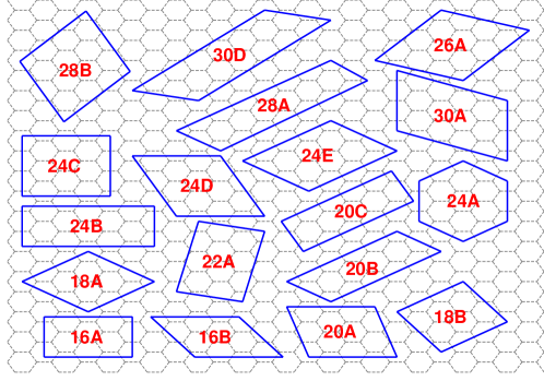
Figure 1: Clusters used in this study.

Further understanding of the latter two phases can be gained by calculating the single-particle occupation at different momentum points

$$n({\bf k})=\braket{\alpha_{\bf k}^{\dagger}\alpha_{\bf k}^{\phantom{{\dagger}}}}+\braket{\beta_{\bf k}^{\dagger}\beta_{\bf k}^{\phantom{{\dagger}}}},$$ (9)

where $\alpha_{\bf k}^{\phantom{{\dagger}}}=\sum_{i\in A}e^{i{\bf k}\cdot{\bf r}_{i}}b_{i}^{\dagger}b_{i}^{\phantom{{\dagger}}}$ and $\beta_{\bf k}^{\phantom{{\dagger}}}=\sum_{i\in B}e^{i{\bf k}\cdot{\bf r}_{i}}b_{i}^{\dagger}b_{i}^{\phantom{{\dagger}}}$ are boson annihilation operators at momentum ${\bf k}$ for the $A$ and $B$ sublattices, respectively. In order to minimize finite-size effects and fully probe the Brillouin zone we average over $40\times 40$ twisted boundary conditions[51, 52],

$$\braket{n({\bf k})}_{\theta_{x},\theta_{y}}=\oint d\theta_{x}\oint d\theta_{y}\braket{n({\bf k},\theta_{x},\theta_{y})},$$ (10)

where $\theta_{\alpha}$ is the flux associated with the twisted boundary condition.

For any finite-size calculation, there are a large number of clusters that one could study, each with slightly different symmetry properties. In this work, we focus solely on clusters that can be described by a parallelogram or “tilted rectangle”. The clusters used in this study are illustrated in figure 1 and are discussed in more detail in [36] and [34].

3 $XY$ Model

In a previous study [34], we reported that the phase diagram of the $XY$ model (1) on a honeycomb lattice has three quantum phase transitions separating four distinct phases. The four phases are: (i) a BEC ${\bf k}=\Gamma$ (antiferromagnetism), (ii) a Bose metal (spin liquid), (iii) a BEC at ${\bf k}=M$ (a collinear spin wave), and (iv) a BEC at ${\bf k}=K$ ($120^{\circ}$ order).

The key signature of a Bose metal is the absence of any order and a singularity in the momentum distribution $n({\bf k})$. In figure 2(a) and 2(b), we show $n({\bf k})$ for two values of $t_{2}/t_{1}$ that are typical for the Bose metal phase. For this phase, $n({\bf k})$ features a $t_{2}/t_{1}$-dependent Bose surface, which, as a guide to the eye, we indicate by a dashed red line. In general, the Bose wave vector $q_{B}$ at which the maxima of $n({\bf k})$ occurs increases with increasing $t_{2}/t_{1}$, as shown in figure 2(c). We emphasize that the maxima in $n({\bf k})$ do not reflect Bose-Einstein condensation as they do not scale with system size.

$\begin{array}[]{ccc}\includegraphics[height=88.53229pt,draft=false]{fig2a.eps}&\includegraphics[height=88.53229pt,draft=false]{fig2b.eps}&\includegraphics*[height=88.53229pt,draft=false,viewport=5.01874pt 11.04124pt 355.3275pt 242.90749pt,draft=false]{fig2c.eps}\end{array}$

Figure 2: (Color online) (a)-(b) Momentum distribution $n({\bf k})$ versus ${\bf k}$ [53] for the Bose metal phase in the $XY$ model for $t_{2}/t_{1}=0.28$ and $0.33$, respectively. In both panels, $40\times 40$ twisted boundary conditions were averaged to generate $n({\bf k})$, and the Bose surface is indicated by a dashed red line. (c) The magnitude of the Bose-surface $q_{B}$ as a function of $t_{2}/t_{1}$.

4 BHH Model

In this work, we present evidence that, in the $(\phi,V)$ plane [see (3)], the Bose-Hubbard-Haldane model for $t_{2}/t_{1}=0.3$ exhibits (at least) three phases at half-filling. For strong coupling $V$, the ground state is a charge-density-wave (CDW), while (at least) two possible ground states exist at weak-coupling. In the frustrated regime ($\phi\sim 0$) at $V=0$, the system favors a Bose-metal, while the unfrustrated regime ($\phi\sim\pi$) favors a BEC. Consequently, we find that there are three types of transitions: (i) BEC-CDW, (ii) BEC-BM, and (iii) BM(other phase)-CDW.

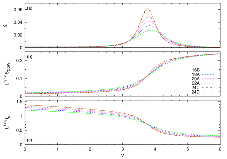
Figure 3: (Color online) (a) Fidelity metric $g$, (b) scaled structure factor $L^{-\gamma/\nu}S_{\rm CDW}$, and (c) scaled condensate fraction $L^{1+\eta}f_{c}$ as a function of interaction strength for various clusters with $\phi=\pi$.

Let us first consider the BEC-CDW transition driven by $V$ at constant $\phi$. In figure 3, we show the properties of the system for $\phi=\pi$. In panel (a), we show the fidelity metric versus $V$, which has a smooth peak that grows with system size, indicative of a second-order phase transition (which would be unconventional in this case in which the system transitions between two ordered states) or a weakly first order transition. If the former is true, the structure factor would scale according to the rule:

$$L^{-\gamma/\nu}S_{\rm CDW}=f[(V-V_{c})L^{1/\nu}],$$ (11)

where $N$ is the number of sites, $L=N^{1/2}$ is the linear dimension, and $\gamma=\nu(2-\eta)$. Because of our small lattice sizes, we cannot pinpoint the exact nature of this transition. For example, using a scaling analysis based on the 3D Ising [54] and $XY$ universality classes [55] yield very similar results. In figure 3(b), we show the CDW structure factor scaled in accordance with the 3D $XY$ universality class, resulting in $V_{c}=3.71(7)$.

We can check the robustness of this result by considering the condensate fraction, which scales [56, 57, 58] according to

$$L^{y}f_{c}=g[(V-V_{c})L^{1/\nu}],$$ (12)

where $y=(d+z-2+\eta)$. This is illustrated in figure 3(c), resulting in $V_{c}=3.73(3)$. This result is quite close to the one obtained using the structure factor. We stress, once again, that although this appears to be a second-order transition between two ordered states, finite-size limitations do not allow us to rule out the possibility of a weak first-order transition or the existence of a small intermediate phase separating the BEC and CDW states.

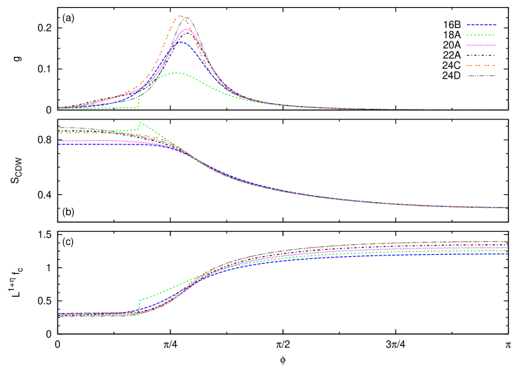
Figure 4: (Color online) (a) Fidelity metric $g$, (b) structure factor $S_{\rm CDW}$, and (c) scaled condensate fraction $L^{1+\eta}f_{c}$ as a function of $\phi$ for various clusters with $V=0$.

Next, we examine the properties of the model as one transitions from the Bose metal to the BEC state. In figure 4, we show the same quantities as in figure 3 (this time versus $\phi$) for $V=0$. The fidelity metric is plotted in figure 4(a), and peaks at approximately $\phi\sim 0.88$. In figure 4(b), we show the structure factor, which does not scale with finite size in either phase. Figure 4(c) depicts the scaled condensate fraction, yielding $\phi_{c}=0.84\pm 0.14$, consistent with the peak in the fidelity metric. (Note that the $18A$ cluster experiences a level crossing for $\phi<\phi_{c}$.) As in the previous case, we cannot make definite statements about the nature of the transition between the Bose metal and the BEC state, but our results are consistent with a second order or a weakly first order transition.

$\begin{array}[]{cccc}\includegraphics[width=99.73074pt,draft=false]{fig5a.eps}&\includegraphics[width=99.73074pt,draft=false]{fig5b.eps}&\includegraphics[width=99.73074pt,draft=false]{fig5c.eps}&\includegraphics[width=99.73074pt,draft=false]{fig5d.eps}\end{array}$

Figure 5: (Color online) Momentum distribution function $n({\bf k})$ versus ${\bf k}$ [53] for $V=0$ and (a) $\phi=0$, (b) $\phi=\pi/9$, (c) $\phi=\pi/4$, and (d) $\phi=\pi/3$.

It is now interesting to study how the Bose surface changes as $\phi$ increases and one transitions between the Bose-metal and the BEC phase. In figure 5, we show the momentum distribution function for four values of $\phi$ and fixed $V=0$. As seen in figure 5(b), the Bose surface reduces in size as $\phi$ departs from zero and continues to shrink until condensation occurs at ${\bf k}=\Gamma$ [see Figs. 5(c) and 5(d)] for $\phi>\phi_{c}$.

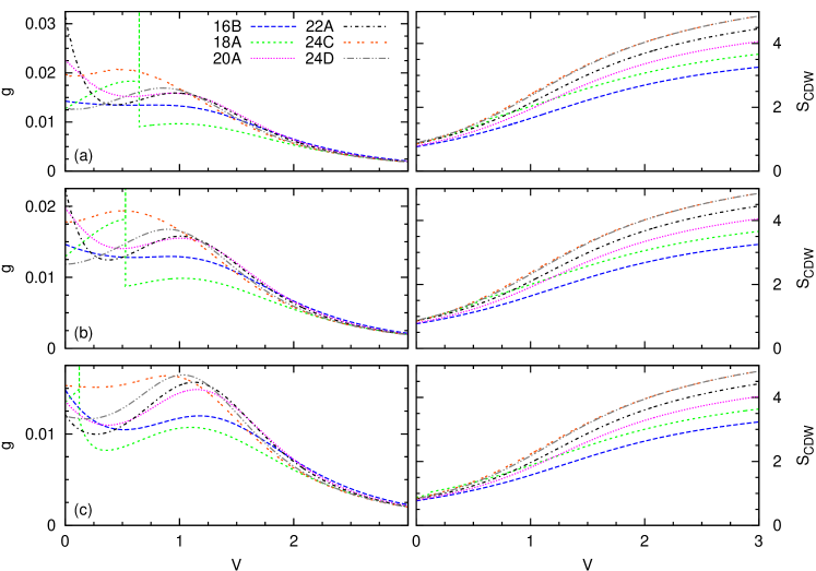
Figure 6: (Color online) Fidelity metric $g$ (left) and structure factor $S_{\rm CDW}$ (right) as a function of interaction strength for various clusters with (a) $\phi=0$, (b) $\phi=\pi/12$, and (c) $\phi=\pi/6$.

A third phase transition is expected as $V$ is increased from zero and the BM phase is destroyed to give rise to the large $V$ CDW phase. We illustrate this regime in figure 6 by plotting the fidelity metric (left panels) and CDW structure factor (right panels) for, (a) $\phi=0$, (b) $\pi/12$, and (c) $\pi/6$. In the left panels, for all three values of $\phi$, one can see a sort of two-peak structure in the fidelity metric.

The large value of $g$ at $V=0$ may be an indicator of a transition away from the Bose metal at $V=0^{+}$. It is somewhat similar to the behavior of $g$ in both the one-dimensional Hubbard model, where the Mott–metal-insulator phase transition occurs for the onsite repulsion $U=0^{+}$ [44], and the two-dimensional hole-doped $t$-$J$ model [45], where $d$-wave superconductivity was seen to develop for a superconducting inducing perturbation with vanishing strength. Another possibility is that the Bose-Metal is stable for positive and small values of $V$, but a transition to another phase occurs when $V<0$. The peak produced by such a transition would also explain the structure we see in $g$. We have also investigated this model with negative values of $V$, and found that large peaks are present in the fidelity metric for $V<0$. The position of those peaks had a strong dependence on the cluster geometry. Hence, exactly what happens to the BM phase in the region $V\sim 0$ is something that requires further studies, maybe with other techniques that allow access to larger system sizes and a better finite size scaling analysis.

For all clusters and values of $\phi$ depicted in the left panels in figure 6, one can also see a clear peak in the fidelity metric for finite values of $V$. This feature indicates the onset of CDW order. The structure factor $S_{\rm CDW}$, depicted in the right panels in figure 6, make apparent that for values of $V$ beyond that peak, the CDW structure factor scales with system size.

$\begin{array}[]{ccc}\includegraphics[height=88.53229pt,draft=false]{fig7a.eps}&\includegraphics[height=88.53229pt,draft=false]{fig7b.eps}&\includegraphics[height=88.53229pt,draft=false]{fig7c.eps}\end{array}$

Figure 7: (Color online) Momentum distribution function $n({\bf k})$ versus ${\bf k}$ [53] with constant $\phi=0$ for (a) $V=0$, (b) $V=0.25$ and (c) $V=1$.

In figure 7, we illustrate how the momentum distribution function changes in the presence of interactions at fixed $\phi=0$. $n({\bf k})$ is shown for $V=0$ in panel (a) and as the interactions are increased in panels (b) and (c). In figure 7(b), one can see that the Bose-surface broadens as $V$ increases and moves closer to ${\bf k}=\Gamma$. Increasing the nearest-neighbor repulsion further, so that the system enters in the CDW phase [figure 7(c)], results in a momentum distribution function that peaked at ${\bf k}=\Gamma$, albeit without condensation. Instead, the structure factor $S({\bf k})$ is sharply peaked at ${\bf k}=\Gamma$.

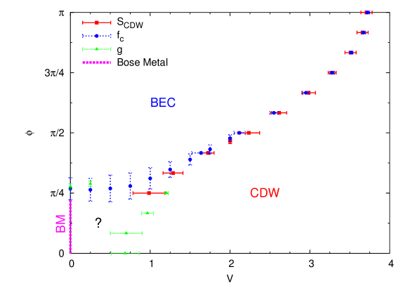
Figure 8: (Color online) Phase diagram for the Bose-Hubbard-Haldane model with parameters $t_{1}=1.0$ and $t_{2}=0.3$. The solid red squares are determined by the crossing point in the scaling of $S_{\rm CDW}$. The solid blue circles are from the crossing point in $f_{c}$. The green triangles are the average of the location of peak in the fidelity metric for the largest system sizes. The Bose Metal (BM) phase is indicated by the thick, dashed magenta line.

A summary of our calculations for different values of $V$ and $\phi$ is presented in figure 8 as the phase diagram of the hard-core BHH model at half-filling with $t_{1}=1.0$ and $t_{2}=0.3$. For $\phi>\pi/4$, the boundary of the CDW phase was identified by the crossing points in the scaling of the structure factor (figure 3). The boundary of the BEC phase was identified by the crossing points in the scaling of the condensate fraction (Figs. 3 and 4), and, for small values of $V$, also using the maximum of the fidelity metric for the largest systems sizes (figure 4). For $\phi<\pi/4$, the CDW transition boundary was determined by the position of the maximum in the peak in the fidelity metric for the largest system sizes (figure 6). Note that, in that regime, the Bose metal phase was found to be stable for $V=0$. On the other hand, for $V$ between 0 and the boundary of the CDW phase, the large value of the fidelity metric, as well as the behavior of several observables studied in that region, prevent us from making a clear statement about the nature of the ground state.

5 Conclusion

In summary, we have studied the phase diagram of the hard-core Bose-Hubbard-Haldane Hamiltonian, which has allowed us to probe the effect of perturbations on the Bose metal phase found in the frustrated $XY$ model on a honeycomb lattice [34]. In particular, we explored the parameter dependence of the Bose wave vector and verified that the Bose metal is stable under the effects of time-reversal and chiral symmetry breaking. We identified three phases in the phase diagram of the BHH model; (I) a Bose metal, (II) a BEC, and (III) a CDW. The phase transitions between the different phases were identified utilizing the ground state fidelity metric, the CDW structure factor, the condensate fraction, and the momentum distribution.

The BEC-CDW transition appears to be second order, although finite-size effects prevent us from ruling out the possibility of a weak first-order transition or the existence of an intermediate phase separating the BEC and the CDW states. If this transition is indeed a direct second order phase transition, the critical point would be highly nontrivial, and could be an example of deconfined criticality.

We have also found that the Bose metal is destroyed upon increasing $V$, before the Heisenberg point for nearest neighbor interactions $V=2J_{1}$ can be reached. The presence of a next-nearest-neighbor repulsion may change this and result in transitions to other exotic phases.

References

- [1] Pomeranchuk I Y 1941 Zh. Eksp. Teor. Fiz. 11 226
- [2] Anderson P W 1987 Science 235 1196–1198
- [3] Lee P A, Nagaosa N and Wen X G 2006 Rev. Mod. Phys. 78 17–85
- [4] Wen X G 2002 Phys. Rev. B 65 165113
- [5] Hermele M, Senthil T, Fisher M P A, Lee P A, Nagaosa N and Wen X G 2004 Phys. Rev. B 70 214437
- [6] Rokhsar D S and Kivelson S A 1988 Phys. Rev. Lett. 61(20) 2376–2379
- [7] Moessner R and Sondhi S L 2001 Phys. Rev. Lett. 86(9) 1881–1884
- [8] Yao H and Kivelson S A 2012 Phys. Rev. Lett. 108(24) 247206
- [9] Kitaev A 2006 Ann. Phys. 321 2 – 111
- [10] Meng Z Y, Lang T C, Wessel S, Assaad F F and Muramatsu A 2010 Nature 464 847
- [11] Yan S, Huse D A and White S R 2011 Science 332 1173–1176
- [12] Okumura S, Kawamura H, Okubo T and Motome Y 2010 Journal of the Physical Society of Japan 79 114705
- [13] Cabra D C, Lamas C A and Rosales H D 2011 Phys. Rev. B 83(9) 094506
- [14] Clark B K, Abanin D A and Sondhi S L 2011 Phys. Rev. Lett. 107(8) 087204
- [15] Mezzacapo F and Boninsegni M 2012 Phys. Rev. B 85(6) 060402
- [16] Kalz A, Arlego M, Cabra D, Honecker A and Rossini G 2012 Phys. Rev. B 85(10) 104505
- [17] Yang H Y, Albuquerque A, Capponi S, Läuchli A and Schmidt K Effective spin couplings in the Mott insulator of the honeycomb lattice Hubbard model arXiv:1207.1072
- [18] Vachon M A, Koutroulakis G, Mitrović V F, Ma O, Marston J B, Reyes A P, Kuhns P, Coldea R and Tylczynski Z 2011 New Journal of Physics 13 093029
- [19] Yan Y J, Li Z Y, Zhang T, Luo X G, Ye G J, Xiang Z J, Cheng P, Zou L J and Chen X H 2012 Phys. Rev. B 85(8) 085102
- [20] Liu D Y, Guo Y, Zhang X L, Wang J L, Zeng Z, Lin H Q and Zou L J Strongly correlated electronic states and quasi-two-dimensional antiferromagnetism in honeycomb lattice compound In3Cu2VO9 arXiv:1202.1861
- [21] Sorella S, Otsuka Y and Yunoki S Absence of a spin liquid phase in the Hubbard model on the honeycomb lattice arXiv:1207.1783
- [22] Wang F 2010 Phys. Rev. B 82(2) 024419
- [23] Lu Y M and Ran Y 2011 Phys. Rev. B 84(2) 024420
- [24] Mulder A, Capriotti R G L and Paramekanti A 2010 Phys. Rev. B 81 214419
- [25] Albuquerque A F, Schwandt D, Hetényi B, Capponi S, Mambrini M and Läuchli A M 2011 Phys. Rev. B 84 024406
- [26] Reuther J, Abanin D A and Thomale R 2011 Phys. Rev. B 84(1) 014417
- [27] Oitmaa J and Singh R R P 2011 Phys. Rev. B 84(9) 094424
- [28] Mosadeq H, Shahbazi F and Jafari S A 2011 Journal of Physics: Condensed Matter 23 226006
- [29] Motrunich O I and Fisher M P A 2007 Phys. Rev. B 75 235116
- [30] Sheng D N, Motrunich O I and Fisher M P A 2009 Phys. Rev. B 79 205112
- [31] Yang H Y, Läuchli A M, Mila F and Schmidt K P 2010 Phys. Rev. Lett. 105(26) 267204
- [32] Dang L, Inglis S and Melko R G 2011 Phys. Rev. B 84(13) 132409
- [33] Mishmash R V, Block M S, Kaul R K, Sheng D N, Motrunich O I and Fisher M P A 2011 Phys. Rev. B 84(24) 245127
- [34] Varney C N, Sun K, Galitski V and Rigol M 2011 Phys. Rev. Lett. 107 077201
- [35] Haldane F D M 1988 Phys. Rev. Lett. 61 2015–2018
- [36] Varney C N, Sun K, Rigol M and Galitski V 2010 Phys. Rev. B 82 115125
- [37] Lanczos C 1950 J. Res. Natl. Bur. Stand. 45 255
- [38] Cullum J K and Willoughby R A 1985 Lanczos Algorithms for Large Symmetric Eigenvalue Computations: Theory vol 1 (Boston: Birkäuser)
- [39] Simon H D 1984 Lin. Alg. Appl. 61 101–131
- [40] Sorenson D C 1992 SIAM. J. Matrix Anal. Appl. 13 357–385
- [41] Calvetti D, Raeichel L and Sorenson D 1994 Elec. Trans. Num. Anal. 2 1–21
- [42] Wu K and Simon H 2000 SIAM. J. Matrix Anal. Appl. 22 602–616
- [43] Zanardi P and Paunković N 2006 Phys. Rev. E 74 031123
- [44] Campos Venuti L, Cozzini M, Buonsante P, Massel F, Bray-Ali N and Zanardi P 2008 Phys. Rev. B 78 115410
- [45] Rigol M, Shastry B S and Haas S 2009 Phys. Rev. B 80 094529
- [46] Gu S J 2010 Int. J. Mod. Phys. B 24 4371–4458
- [47] Penrose O and Onsager L 1956 Phys. Rev. 104 576–584
- [48] Yang C N 1962 Rev. Mod. Phys. 34(4) 694–704
- [49] Leggett A J 2001 Rev. Mod. Phys. 73 307–356
- [50] Stanescu T D, Anderson B and Galitski V 2008 Phys. Rev. A 78 023616
- [51] Poilblanc D 1991 Phys. Rev. B 44 9562–9581
- [52] Gros C 1992 Z. Phys. B 86(3) 359–365
- [53] The momentum distribution n(k) illustrated in figures 2, 5, and 7 were calculated for the cluster. All clusters studied here are depicted in figure 1.
- [54] Hasenbusch M 2010 Phys. Rev. B 82(17) 174433
- [55] Campostrini M, Hasenbusch M, Pelissetto A and Vicari E 2006 Phys. Rev. B 74(14) 144506
- [56] Binder K 1981 Z. Phys. B 43 119
- [57] Brézin E and Zinn-Justin J 1985 Nucl. Phys. B 257 867
- [58] Rath S P and Zwerger W 2010 Phys. Rev. A 82 053622