Relaxation dynamics in type-II superconductors with point-like and correlated disorder

Abstract

We employ an elastic line model to investigate the steady-state properties and non-equilibrium relaxation kinetics of magnetic vortex lines in disordered type-II superconductors using Langevin molecular dynamics (LMD). We extract the dependence of the mean vortex line velocity and gyration radius as well as the mean-square displacement in the steady state on the driving current, and measure the vortex density and height autocorrelations in the aging regime. We study samples with either randomly distributed point-like or columnar attractive pinning centers, which allows us to distinguish the complex relaxation features of interacting flux lines subject to extended vs. uncorrelated disorder. Additionally, we find that our new LMD findings match earlier Monte Carlo (MC) simulation data well, verifying that these two microscopically quite distinct simulation methods lead to macroscopically very similar results for non-equilibrium vortex matter.

1 Introduction

Technical applications of type-II superconductors, especially in high-field configurations, require effective pinning mechanisms to prevent flux creep and flow and to thereby avoid dissipative losses. A disordered system of vortex lines at a finite temperature, subject to pinning from randomly distributed point-like or correlated pinning sites, forms a remarkably complex system displaying a wealth of features. Naturally occurring weak point-like disorder already destroys the low-temperature Abrikosov lattice present in a clean system in favor of a new Bragg glass phase with quasi long-range positional order. The first-order melting transition Nelson1988 ; Nelson1989 ; Nelson1989a is then replaced by a continuous transition into a vortex glass phase Fisher1989 ; Fisher1991 ; Feigelman1989 ; Nattermann1990 , in which translational order is completely lost. Hence, vortex matter with weak, randomly placed, point-like disorder already shows a very rich phase diagram Blatter1994 ; Banerjee2001 . The introduction of correlated disorder, such as columnar pinning sites, results in a strongly pinned Bose glass phase with localized vortex lines and a diverging tilt modulus Nelson1992 ; Lyuksyutov1992 ; Nelson1993 , which is accessible to analytical treatment via a mapping to the propagation of bosons in imaginary time Fisher1989a ; Tauber1997 .

Since Struik’s original investigation on physical aging in various materials Struik1978 , many glassy systems have been found to show physical aging Henkel2007 . More recent studies confirm that many other systems show the characteristics of glass-like relaxation and aging Henkel2010 ; Cugliandolo2003 ; Henkel2008 . Experimentally, Du et al. detected evidence of physical aging in disordered vortex matter by demonstrating that the voltage response of a 2H-NbSe₂ sample to a current pulse depends on the pulse duration Du2007 . Thin-film Monte Carlo relaxation and aging studies of a coarse-grained two-dimensional model were performed by Nicodemi and Jensen Nicodemi2002 ; Nicodemi2001a ; Jensen2001 ; Nicodemi2001 . Bustingorry, Cugliandolo and Domínguez investigated the relaxation of vortex matter employing Langevin molecular dynamics (LMD) for a three-dimensional line model, finding clear indications of physical aging in two-time quantities such as the density-density autocorrelation function, the linear susceptibility and the mean-square displacement Bustingorry2006 ; Bustingorry2007 .

In this paper, we report the results of a study comparing the non-equilibrium relaxation kinetics of vortex lines in the presence of randomly distributed point-like disorder and correlated columnar disorder. The origin of point-like pinning sites can be either naturally occurring, or artificially introduced crystal defects. Similarly, correlated columnar disorder appears either as line dislocations or in the form of material damage tracks stemming from high-energy ion irradiation. It is well-established experimentally that columnar disorder yields considerably enhanced pinning efficiency over uncorrelated point-like disorder Civale1991 . Since linear pinning centers are extended along one spatial dimension, one also expects profound differences in the out-of-equilibrium relaxation of magnetic flux lines as compared to samples with randomly distributed point pins. Naturally, these differences can only be addressed in a fully three-dimensional model and numerical study.

We perform extensive Langevin molecular dynamics simulations on a coarse-grained elastic line model of vortex matter. For non-equilibrium systems, it is important to compare and thus validate different microscopic realizations and simulation methods, in order to ascertain that the resulting macroscopic features stem from physical properties of the system and not from artifacts of the specific algorithm. We first present our LMD data on the steady-state vortex velocity and radius of gyration for driven flux lines subject to point-like or columnar disorder. To validate our simulation code, we compare these results for attractive point pins with earlier findings from Monte Carlo (MC) simulations. We proceed to systematically investigate the complex non-equilibrium relaxation behavior of a system of initially randomly distributed and perfectly straight vortex lines via various two-time observables. For point-like disorder, we again compare our novel LMD results with previously published MC data Pleimling2011 . The main focus of this work is the distinct relaxation behavior of flux lines in the presence of randomly distributed columnar and point pinning centers.

Our paper is organized as follows: In the next Section we define and explain the elastic line model as well as our LMD algorithm and discuss the values of the different system parameters. We then introduce the quantities that we are using in order to understand the non-equilibrium properties of interacting vortex lines in the presence of different types of attractive defects. Section 3 is devoted to a discussion of the steady-state properties. We use this regime in order to validate the different algorithms used for the study of our system. Section 4 presents our numerical results. In a systematic study we disentangle the different effects due to the line tension, the vortex-vortex interaction, the pinning to defect sites, and the finiteness of the system. We discuss our main finding on how the different types of pinning centers, point-like and extended columnar defects, affect the non-equilibrium relaxation process. Finally, we summarize our results in Section 5.

2 Model and Simulation Protocol

2.1 Effective Model Hamiltonian

We consider in the following a system of $N$ vortex lines in the London limit, where the penetration depth is much larger than the coherence length. In order to model the dynamics of the system we employ a fully three-dimensional elastic line description Nelson1993 ; Das2003 . The Hamiltonian of this system is written as a functional of the vortex line trajectories $\vec{r}_{i}(z)=\bigl{(}x_{i}(z),y_{i}(z)\bigr{)}$, where $z$ denotes the direction of the applied external magnetic field, and consists of three competing terms: the elastic line energy, the attractive external potential due to disordered pinning sites, and the repulsive vortex-vortex interactions:

$$\begin{split}H\left[\vec{r}_{i}(z)\right]=&\sum_{i=1}^{N}\int_{0}^{L}dz\Biggl{[}\frac{\tilde{\epsilon}_{1}}{2}\left|\frac{d\vec{r}_{i}(z)}{dz}\right|^{2}+U_{D}(\vec{r}_{i}(z),z)\\ &+\frac{1}{2}\sum_{j\neq i}^{N}V(|\vec{r}_{i}(z)-\vec{r}_{j}(z)|)\Biggr{]}.\end{split}$$ (1)

The elastic line stiffness or local tilt modulus is given by $\tilde{\epsilon}_{1}\approx\Gamma^{-2}\epsilon_{0}\ln(\lambda_{ab}/\xi_{ab})$, where $\Gamma^{-1}=M_{ab}/M_{c}$ represents the effective mass ratio or anisotropy parameter, whereas $\lambda_{ab}$ and $\xi_{ab}$ respectively denote the London penetration depth and coherence length in the $ab$ crystallographic plane. The in-plane vortex-vortex interaction is given by $V(r)=2\epsilon_{0}K_{0}(r/\lambda_{ab})$, with the zeroth-order modified Bessel function $K_{0}$ (essentially a logarithmic repulsion that is exponentially screened at the scale $\lambda$). In our simulations, the interaction is cut off at $5\lambda_{ab}$ in order to avoid artifacts due to the periodic boundary conditions. The $N_{D}$ pinning sites are modeled by randomly distributed smooth potential wells of the form

$$\begin{split}U_{D}(\vec{r},z)\!=\!-\!\!\sum_{\alpha=1}^{N_{D}}\!\frac{b_{0}}{2}p\,\delta(z-z_{\alpha})\!\!\left[1\!-\!\tanh\left(\!5\frac{\left|\vec{r}-\vec{r}_{\alpha}\right|-b_{0}}{b_{0}}\!\right)\right],\end{split}$$

where $p\geq 0$ is the pinning potential strength, and $\vec{r}_{\alpha}$ and $z_{\alpha}$ indicate the in-plane and $z$ position of pinning site $\alpha$. Lengths are measured in units of the pinning potential width $b_{0}$. Energies are measured in units of $\epsilon_{0}b_{0}$ with $\epsilon_{0}=(\phi_{0}/4\pi\lambda_{ab})^{2}$, and the magnetic flux quantum $\phi_{0}=hc/2e$.

2.2 Langevin Molecular Dynamics

We employ a LMD algorithm to simulate the vortex line dynamics. To this end, we discretize the system into layers along the $z$ axis. The layer spacing corresponds to the crystal unit cell size $c_{0}$ along the crystallographic c-direction Das2003 ; Bullard2008 . Forces acting on the vortex line vertices can then be derived from the properly discretized version of the Hamiltonian (1). We proceed to numerically solve the (overdamped) Langevin equation

$$\eta\frac{\partial\vec{r}_{i}(t,z)}{\partial t}=-\frac{\delta H[\vec{r}_{i}(t,z)]}{\delta\vec{r}_{i}(t,z)}+\vec{f}_{i}(t,z).$$ (2)

with the Bardeen-Stephen viscous drag parameter $\eta$. The fast, microscopic degrees of freedom of the surrounding medium are captured by thermal stochastic forcing, modeled as uncorrelated Gaussian white noise fulfilling $\left<\vec{f}_{i}(t,z)\right>=0$ and the Einstein relation $\left<\vec{f}_{i}(t,z)\vec{f}_{j}(s,z^{\prime})\right>=2\eta k_{\rm B}T\delta_{ij}\delta(t-s)\delta(z-z^{\prime})$, which guarantees that the system relaxes to thermal equilibrium with a canonical probability distribution $\propto e^{-H/k_{\rm B}T}$. The time integration is performed via simple discretization of Eq. (2) Brass1989 .

2.3 Monte Carlo Algorithm

In section 3, we will compare steady-state results of systems of driven vortex lines generated by our LMD algorithm to data stemming from MC simulations. The MC data was obtained by applying the standard Metropolis update rule to the Hamiltonian (1): A line element is picked at random and made to jump in a random direction and (but truncated) distance. The ensuing change in the system’s energy $\Delta E$ is then evaluated and the Metropolis rule then accepts the jump with a probability $P(\Delta E)=\min\{1,\exp(-\Delta E/k_{B}T)\}$. One MC step is completed when exactly $NL$ line elements have been selected.

2.4 Material Parameters

We chose our simulation parameters to closely match the material parameters of the ceramic high-$T_{C}$ type-II superconducting compound YBa₂Cu₃O₇ (YBCO). The material is highly anisotropic with an effective mass anisotropy ratio of $\Gamma^{-1}=1/5$. We set the pinning center radius to $b_{0}=35\text{\AA}$ and measure simulation distances in terms of this length. The in-plane London penetration depth and coherence length are $\lambda_{ab}=34b_{0}\approx 1200\text{\AA}$ and $\xi_{ab}=0.3b_{0}\approx 10.5\text{\AA}$ respectively. The vortex line energy per unit length is $\epsilon_{0}\approx 1.92\cdot 10^{-6}\operatorname{erg}/\operatorname{cm}$, hence the line tension energy scale becomes $\tilde{\epsilon}_{1}\approx 0.189\epsilon_{0}$. The depth of the pinning center potential is set to $p=0.05\epsilon_{0}$, except when noted differently. To fix the intrinsic simulation time scale, we set the Bardeen-Stephen viscous drag coefficient $\eta=\phi_{0}^{2}/2\pi\rho_{n}c^{2}\xi_{ab}^{2}\approx 10^{-10}\operatorname{erg}\cdot\operatorname{s}/\operatorname{cm}^{2}$ to one (for the normal-state resistivity of YBCO near $T_{C}$, $\rho_{n}\approx 500\mu\Omega\operatorname{cm}$, see table 1 in Ref. Abdelhadi1994 ), resulting in a basic time unit of $t_{0}=\eta b_{0}/\epsilon_{0}\approx 18\operatorname{ps}$.

2.5 Relaxation Simulation Protocol

Throughout our study, the investigated systems contained $N=16$ vortex lines with $L=640$ number of layers (except where noted differently). In the scenarios that include disorder, the number of pinning sites per layer is $N_{D}/L=1116$ which corresponds to a mean in-plane distance of $9b_{0}$ between pinning sites. In the case of randomly arranged point defects, the pinning site positions are chosen anew for each layer, whereas for columnar disorder, each layer repeats the pattern of the first layer’s randomly chosen positions. The system size is set to $(16/\sqrt{3})\lambda_{ab}\times 8\lambda_{ab}$, with the aspect ratio chosen such that a clean system with interacting vortex lines reproducibly forms a hexagonal Abrikosov lattice configuration after equilibration. We employ periodic boundary conditions in the $x$ and $y$ directions, and free boundary conditions along the $z$ axis.

Our initial out-of-equilibrium condition consists of a system of perfectly straight vortex lines, placed at random locations throughout the computational domain. Since the vortex line elements do not yet fluctuate (i.e. their distance from the vortex line mean in-plane position is zero), the internal vortex line configuration effectively is at zero temperature, hence, the start of the simulation at $t=0$ is similar to an up-quench to a finite temperature $T=10\operatorname{K}$. This is in contrast to their random spatial distribution, which is equivalent to an infinite temperature. We then let the system relax towards equilibrium until the waiting time $t=s$ (typically in the range of $2$ to $4096$) is reached, when we take a snapshot of the system. We proceed to calculate various two-time quantities (see section 2.6 below) at logarithmically-spaced time intervals with a simulation end time that is ten times larger than the waiting time.

2.6 Measured Quantities

In the steady state of our driven flux line system, we measure the mean vortex velocity $v$ by extracting the velocities of each line element in the direction of the driving force $F_{d}$ from the time stepping algorithm in LMD and average over all line elements in the system. In MC, we take the average displacement in the direction of the driving force $F_{d}$ over 30 MC steps and calculate the mean velocity. Using Faraday’s law, we can relate the vortex line mean velocity to an induced electric field $\vec{E}=\vec{B}\times\vec{v}/c$, which translates to a voltage drop across the sample. Similarly, the driving force is related to an applied external current via the Lorentz force $F_{d}=|\vec{j}\times\phi_{0}\vec{B}/B|$. Hence, a driving force vs. mean vortex velocity graph is equivalent to experimentally determined current-voltage (I-V) characteristics.

To quantify thermal spatial fluctuations along the vortex lines, we compute the vortex line radius of gyration $r_{g}=\sqrt{\left<(\vec{r}_{i,z}-\overline{\vec{r}}_{i})^{2}\right>}$, i.e. the root mean-square displacement from the lines’ mean lateral positions. The angular brackets again indicate an average over line elements as well as noise and disorder realizations. This quantity is expected to show a maximum at driving forces just below the depinning transition.

To further accurately capture the relaxation and aging dynamics of out-of-equilibrium disordered vortex line systems, we measure two-time correlation quantities. Since we wish to compare the relaxation behavior in LMD with previously measured MC data, we utilize the same two-time observables as in Ref. Pleimling2011 : the height-height autocorrelation function of the vortex lines, the two-time mean-square displacement and the density-density autocorrelation function. All these quantities depend on two times, labeled in the following as $s$ and $t$, with $s<t$.

The roughness or height-height autocorrelation function of the vortex lines is defined by:

$$C(t,s)=\left<\left(\vec{r}_{i,z}(t)-\overline{\vec{r}}_{i}(t)\right)\left(\vec{r}_{i,z}(s)-\overline{\vec{r}}_{i}(s)\right)\right>,$$ (3)

where $\vec{r}_{i,z}(t)$ are the in-plane coordinates of line $i$ at layer $z$ at time $t$, $\overline{\vec{r}}_{i}(t)$ is the mean position of line $i$, and the averages are taken over all line elements as well as noise and disorder realizations. This quantity contains information about local thermal fluctuations of vortex line elements around the flux line’s mean lateral position. In the case of free, non-interacting vortices, it can be mapped to the height correlation of growing one-dimensional interfaces (see Sec. 4.1).

The two-time mean square displacement, defined as

$$B(t,s)=\left<(\vec{r}_{i,z}(t)-\vec{r}_{i,z}(s))^{2}\right>\;,$$ (4)

measures the average square distance between a vortex line element’s position at time $s$ and a subsequent time $t$. This quantity provides data on the time evolution of the global structure of the vortex line configuration, in addition to the same local information contained in $C(t,s)$.

Finally, the two-time density-density autocorrelation function $C_{v}(t,s)$ is an observable that is measured by saving a snapshot of the positions of all vortex line elements in the system at time $s$, calculating the radial distance $r_{i}(t,s)$ each vortex line element traveled between times $s$ and $t$ and determining the number $n_{c}$ of vortex line elements for which this distance is smaller than a prescribed cutoff distance $r_{i}(t,s)<r_{c}$. The density autocorrelation is then $C_{v}(t,s)=\left<n_{c}/NL\right>$. Throughout our study, the cutoff distance is $r_{c}=0.05b_{0}$. The density autocorrelation also contains information on the formation or decay of global structures; thus we expect it to generally follow the behavior of $B(t,s)$.

2.7 Comparison of Microscopic Algorithms

In order to simulate the dynamics of elastic lines in a disordered medium, an appropriate microscopic algorithm has to be chosen. A considerable amount of work has been done using Metropolis MC implementations of the model described above and variations thereof Das2003 ; Bullard2008 ; Klongcheongsan2010 . Gotcheva et al. investigated the differences between a Metropolis and a continuous-time MC algorithm for a system of flux lines on a discrete lattice and subject to varying temperature and driving force Gotcheva2004 ; Gotcheva2005 . The continuous-time update rule preserved positional order, while the Metropolis rule led to a disordered moving state, questioning the validity of the Metropolis algorithm for studies of driven vortex matter in lattice simulations. More recent studies demonstrated that positional order was preserved in off-lattice Metropolis MC of driven vortex matter Bullard2008 .

It is crucial to investigate and compare different microscopic implementations of algorithms such as Metropolis MC and LMD simulations in a non-equilibrium setting. The choice of algorithm might introduce spurious effects that cannot be predicted a priori. In order to separate actual physical effects of the studied elastic line model from these artifacts, we performed a careful numerical comparison of LMD with earlier MC studies. Fast microscopic degrees of freedom are modeled by the thermal force term in LMD, see Eq. (2). In equilibrium the noise strength is set by the Einstein relation (fluctuation-dissipation theorem, FDT). In out-of-equilibrium situations, there exists in general no FDT-equivalent that would uniquely determine the form and strength of the noise correlations. Since the large-scale and long-time characteristics of Langevin stochastic differential equations can be drastically influenced by the noise correlator properties, it is necessary to validate results by comparing to other numerical methods Bullard2008 . In the first part of this article, we therefore compare results from a MC study for both steady-state and relaxation properties of the vortex line model to data generated by the LMD algorithm. It should be noted that a direct comparison of time scales is difficult since the length of a MC time step is a dynamically generated quantity, whereas in LMD the time step duration is a function of the material parameters.

3 Steady-state properties

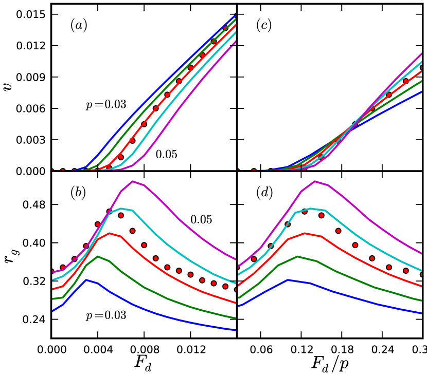
Figure 1: (Color online) Steady-state (a) velocity and (b) gyration radius of $N=16$ vortex lines with a length of $L=20$ elements as a function of the driving force $F_{d}$ in the presence of point pins with varying disorder potential strength $p$. The red circles show data from MC simulations with $p=0.05\epsilon_{0}$, while the other graphs display LMD simulation data with $p$ ranging from $0.03\epsilon_{0}$ to $0.05\epsilon_{0}$ in steps of $0.005\epsilon_{0}$. In (c) and (d), the force axis is rescaled with the disorder potential strength. The velocity curves in (c) cross at $F_{d}/p\approx 0.19$ while the gyration radius maxima in (d) align around $F_{d}/p\approx 0.12$, with a slight bias towards higher $F_{d}/p$ for higher values of $p$.

We first employ LMD simulations for interacting flux lines in the presence of point-like disorder with disorder potential strength $p$, subject to a driving force $F_{d}$ stemming, via the Lorentz force, from an external current. Results for the steady-state velocity and gyration radius are gathered in Fig.  1. The red dots in Fig. 1 indicate MC-generated data, while the solid lines were produced using LMD with different values of $p$. It is quite clear from Fig. 1(a) that a pinning potential strength $p=0.05\epsilon_{0}$ in MC corresponds to $p\approx 0.04\epsilon_{0}$ in LMD. In MC, vortex line elements test a region with a radius of $0.25b_{0}$ around their current position for possible jump targets. It is conceivable that the pin energy barrier appears a bit smoother in MC since its width falls into the same length scale, which leads to the observed renormalization of the pinning potential strength. The slightly higher maximum of the MC gyration radius data for $p=0.05\epsilon_{0}$ over the corresponding LMD curve with $p=0.04\epsilon_{0}$ in Fig. 1(b) supports this argument, since vortex line elements are most likely trapped at a pinning site until they escape via a single jump. It is much less probable for any line element to escape the pin via multiple successive jumps. In LMD on the other hand, the thermal force is only an added component on top of the (in this case stronger) driving and elastic tension forces. Hence, LMD yields smooth escape trajectories out of a point pin’s binding potential, and the vortex line is consequently less rough, resulting in a smaller radius of gyration.

Figures 1(c) and (d) show that the depinning force scales roughly linear with the pinning potential strength $p$, as expected Nelson1993 . The vortex velocity curves cross at $F_{d}/p\approx 0.19$, while the gyration radii have their maxima around $F_{d}/p\approx 0.12$, with a slight systematic shift to lower $F_{d}/p$ for smaller pinning strength values $p$. It should be noted that a true continuous non-equilibrium depinning phase transition occurs only at $T=0$ (and in the thermodynamic limit). The scaling behavior of the velocity of driven vortex lines near the critical depinning force in the presence of point-like disorder has been explored by Luo and Hu Luo2007 . The gyration radius maximum in the vicinity of the critical depinning force may consequently be understood as the thermally rounded remnant of this zero-temperature phase transition Fisher1998 .

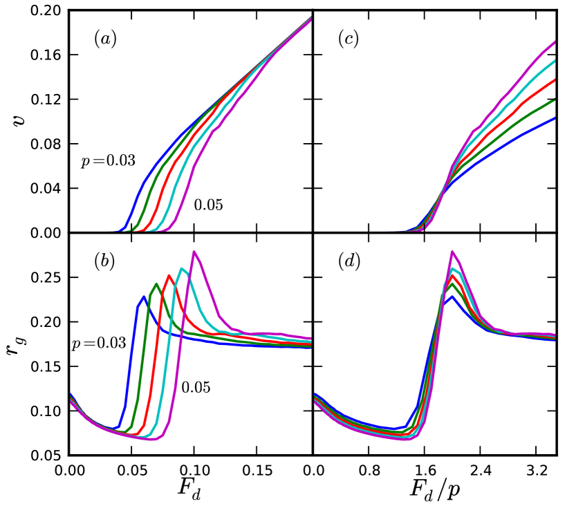
Figure 2: (Color online) Steady-state (a) velocity and (b) gyration radius of $N=16$ vortex lines with $L=20$ as a function of the driving force $F_{d}$ in the presence of columnar disorder, with a disorder potential strength varying between $p=0.03\epsilon_{0}$ and $p=0.05\epsilon_{0}$ in steps of $0.005\epsilon_{0}$. As expected, the radius of gyration displays quite different behavior for columnar pins as compared to point pinning sites, compare Fig. 1(b). In (c) and (d), the force axis is rescaled with the disorder potential strength. The velocity curves in (c) cross at $F_{d}/p\approx 1.9$, while the gyration radius maxima in (d) align around $F_{d}/p\approx 2$.

Figures 2(a) and (b) display the mean velocity $v$ and the radius of gyration $r_{g}$ as a function of the driving force $F_{d}$ of vortices subject to randomly distributed columnar pinning sites. Correlated disorder is much more effective at pinning flux lines than point disorder Civale1991 . This is reflected in a critical depinning force that is about an order of magnitude higher for columnar defects than for uncorrelated point pins of the same strength $p$ (per layer; results shown in Fig. 1). In Figs. 2(c) and (d) the driving force is again scaled with the pin strength $p$. The vortex velocity curves cross at $F_{d}/p\approx 1.9$, which is indeed a factor of $10$ larger compared to point pins. In the presence of columnar defects, a single flux line may be in one of the following four configurations: Nelson1993 (i) unpinned, located away from any pinning sites; (ii) trapped at a single columnar pin for its entire length; (iii) forming a vortex half-loop where the elastic line is trapped at a single columnar defect, with the exception of an unpinned section that extends away from the defect line: Depending on the relative strengths of the driving force, thermal noise, and the pinning potential, the unpinned part may either expand or retract. This state represents a short-lived saddle-point configuration; (iv) forming single or double kinks by being simultaneously trapped at two adjacent pinning columns. This state is rather long-lived but will ultimately decay into either the unpinned or completely trapped state.

The gyration radius indicates which configurations are typically assumed by the vortex lines. For $F_{d}=0$, most vortex lines are fully trapped. The radius of gyration of a trapped line is restricted by the pinning potential extension $b_{0}$, hence we observe a marked reduction in the value of $r_{g}$ with columnar pins over free, unbound lines. With increasing but below-critical $F_{d}$, $r_{g}$ decreases since the mean position of trapped vortex lines shifts from the center of the pinning site, which further constrains fluctuations. In the vicinity of the critical depinning force, in the flux creep regime, $r_{g}$ rises sharply due to the formation of half-loops, single-, and double-kinks. Near the transition to free-flowing flux lines, $r_{g}$ develops a maximum and gradually decreases for even higher $F_{d}$. In this state, vortex motion is slightly restricted by pinning centers, but the flux lines move essentially unimpeded, and the radius of gyration approaches its unbound value.

4 Relaxation processes

In order to study the relaxation dynamics and possible aging scaling of a system of vortex lines in various scenarios, we follow the procedures outlined in Ref. Pleimling2011 . As a test case for our simulation code, we first investigate a system of non-interacting lines without disorder, which can be mapped to the one-dimensional Edwards-Wilkinson (EW) interface growth model. We then proceed to non-interacting lines in the presence of point-like disorder with two different pin potential strengths, where the short-time behavior is similar to the clean system while the long-time relaxation is modified by the attractive defects. To disentangle the effects of the mutual vortex repulsion from the disorder influence, we next study a system of interacting vortex lines without pinning sites. Subsequently, we present data on the full system of interacting vortex lines in the presence of point pinning centers. We then point out the differences in the relaxation kinetics in systems with point and correlated extended pins by investigating both non-interacting and interacting flux lines in the presence of columnar defects. Finally, we discuss finite-size effects due to short vortex lengths for both types of pinning sites.

In each of the scenarios presented below, we first look at the relaxation of the single-time mean-square displacement $B(t,0)$, the time-dependent squared radius of gyration, $r_{g}^{2}(t)$, and the associated effective exponents $\beta_{B}(t)=d\ln B(t,0)/d\ln t$ and $\beta_{h}(t)=d\ln r_{g}^{2}(t)/d\ln t$. The mean-square displacement predominantly probes changes in the average positions of single vortices. Hence we use the average of $\beta_{B}$ over an appropriate time interval as the aging exponent that we utilize to achieve (approximate) data collapse of the two-time global mean-square displacement $B(t,s)$ and density autocorrelation function $C_{v}(t,s)$. The time-dependent radius of gyration describes internal thermal vortex line fluctuations and enables us to compute an averaged scaling exponent $\beta_{h}$ that can be used for obtaining data collapse of the two-time height autocorrelation function $C(t,s)$.

4.1 Free Non-interacting Vortex Lines

The thermal fluctuations of the segment locations of free (non-interacting and not subject to disorder) directed elastic lines around their mean in-plane position can be mapped to the problem of a one-dimensional interface growing via random deposition. The continuous version of this growth model is described by the stochastic Edwards-Wilkinson (EW) equation Edwards1982 . The temporal evolution of the interface height relative to its mean height is governed by a diffusive term as well as a random noise term. Hence, it may be described mesoscopically by a linear Langevin equation,

$$\frac{\partial h(z,t)}{\partial t}=\nu\frac{\partial^{2}h(z,t)}{\partial z^{2}}+\eta(z,t)\;,$$ (5)

where $\nu$ is the diffusive strength and $\eta(z,t)$ represents thermal white noise with zero mean and second moment $\left<\eta(z,t)\eta(z^{\prime},s)\right>=2k_{\rm B}T\nu\delta(z-z^{\prime})\delta(t-s)$ that satisfies Einstein’s relation. The temperature $T$ enters through the noise strength.

The linear nature of Eq. (5) makes it possible to arrive at analytical expressions for various two-time quantities Rothlein2007 ; Bustingorry2007 ; Bustingorry2007a ; Chou2010 . In particular, the solution for the two-time height-height autocorrelation function in the correlated growth regime reads Rothlein2007 ,

$$C(t,s)=C_{0}s^{1/2}\left(\left[\frac{t}{s}+1\right]^{1/2}-\left[\frac{t}{s}-1\right]^{1/2}\right)\;.$$ (6)

Comparing with the general scaling form $C(t,s)=s^{-b}f_{C}(t/s)$ (with scaling function $f_{C}$), this predicts the universal aging exponent $b=1/2$ in the EW regime Pleimling2011 ; Rothlein2007 . The mean square displacement follows a similar scaling form $B(t,s)=s^{-b}f_{B}(t/s)$, while the density autocorrelation empirically scales as $C_{v}(t,s)=s^{b}f_{C_{v}}(t/s)$.

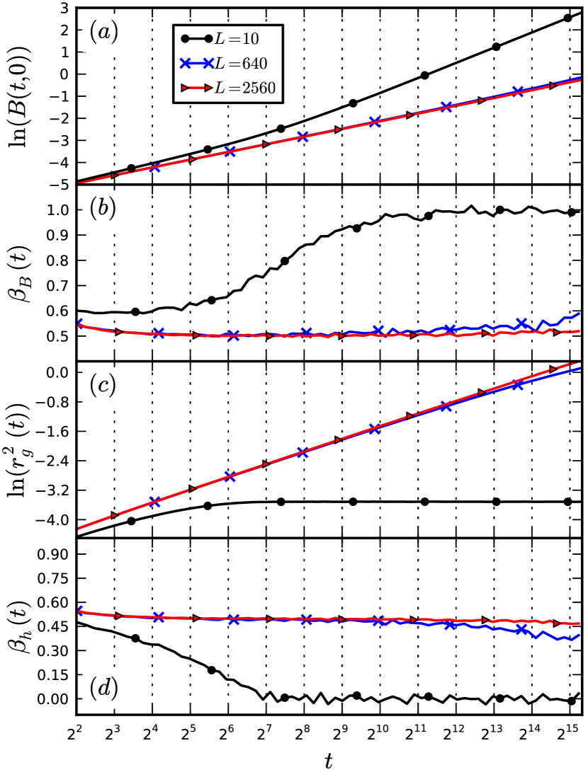
Figure 3: (Color online) Relaxation behavior of (a) the vortex line mean-square displacement $B(t,0)$, (c) the squared gyration radius $r_{g}^{2}(t)$, and (b,d) the associated effective exponents $\beta_{B}$ and $\beta_{h}$ over time for free non-interacting flux lines with length $L=10$ ($\bullet$ marker), $L=640$ ($\times$ marker) and $L=2560$ ($\blacktriangleright$ marker) averaged over at least 1000 realizations.

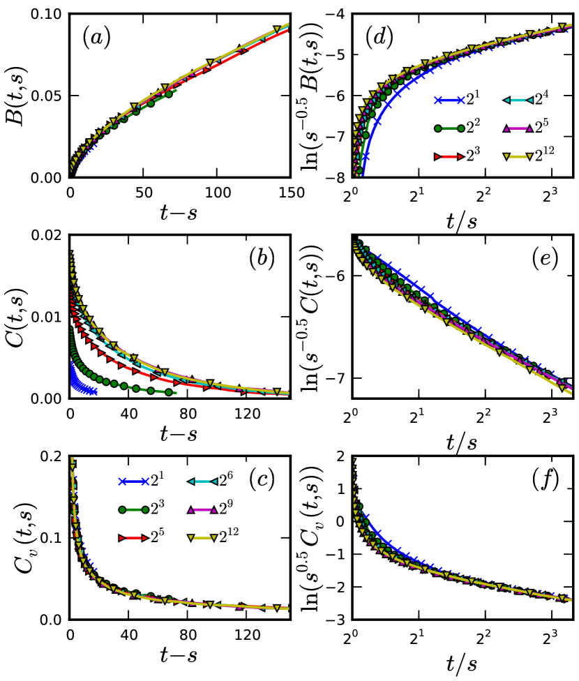
Figure 4: (Color online) Relaxation of two-time quantities in a system of non-interacting flux lines without disorder for a line length of (a-c) $L=10$ and (d-f) $L=2560$, averaged over $800$ different noise realizations. The sub-figures show (a,d) the mean-square displacement $B(t,s)$, (b,e) the height autocorrelation function $C(t,s)$, and (c,f) the density autocorrelation function $C_{v}(t,s)$ as a function of (a-c) $t-s$ and (d-f) $t/s$. Waiting times range from $s=2$ to $2^{12}=4096$. For $L=10$, the system rapidly reaches equilibrium. The height autocorrelation function in (b) displays a short time window ($s<64$) where it explicitly depends on $s$ and time translation invariance is broken. For $L=2560$ and $s>16$, all quantities show aging and dynamical scaling with the EW exponent $b=0.5$.

The relaxation of the observables $B(t,0)$, $r_{g}^{2}(t)$ and the three two-time correlation functions $B(t,s)$, $C(t,s)$, and $C_{v}(t,s)$ in this scenario as observed in our LMD simulations is presented in Figs. 3 and 4, respectively. For a very thin system with $L=10$, we immediately see from the time evolution of the effective exponent $\beta_{B}(t)$ [solid line with black circles in Fig. 3(b)] that the system starts to cross over into equilibrium where $B(t,0)\sim t$, $\beta_{B}\to 1$ for early times $t>2^{5}$, and it is truly equilibrated after $t>2^{10}$. This is also visible in the unscaled two-time quantities $B(t,s)$ and $C_{v}(t,s)$ displayed in Figs. 4(a,c): For $s>2^{4}$, the data of $B(t,s)$ for different waiting times $s$ fall onto a single master curve, which indicates the recovery of time translation invariance. In contrast, the data for $C_{v}(t,s)$ collapse for all waiting times $s$. The difference in the onset of data collapse in these two quantities is caused by local thermal fluctuations contributing to the mean-square displacement, whereas short-scale variations are effectively averaged out due to the finite cutoff radius in the density autocorrelation. The effective gyration radius exponent $\beta_{h}(t)$, displayed in Fig. 3(d), decreases from the start and eventually reaches zero around $t\approx 2^{7}$. For such a short flux line length, the crossover from the EW regime to the saturated (equilibrated) regime happens at very early times. The two-time height-height autocorrelation function $C(t,s)$, plotted in Fig. 4(b), shows data collapse for waiting times $s>2^{7}$, which reflects the time evolution of $\beta_{h}(t)$.

The extended, bulk-like system with $L=2560$ exhibits much slower relaxation and hence enables us to study the dynamical aging scaling regime. The effective exponents $\beta_{B}(t)$ and $\beta_{h}(t)$ [solid lines with black triangles in Figs. 3(b,d)] show the remnants of a crossover for short times, while staying at a value of approximately $0.5$ for $t>2^{4}$. Figures 4(d-f) depict $B(t,s)$, $C(t,s)$ and $C_{v}(t,s)$ respectively as functions of $t/s$ and scaled with appropriately chosen exponents of the waiting time. The data for all three quantities show data collapse for $s>2^{4}$ with exponent $b=0.5$, indicating dynamical scaling and hence full aging in this time regime. The aging exponent of the two-time height-height autocorrelation function coincides with the predicted EW value from Eq. (6).

Except for the early-time crossover between the EW and saturation regimes, which is not visible in Fig. 3 in Ref. Pleimling2011 , our findings produced via LMD simulations are in complete agreement with the MC data for both thin and extended “bulk” systems.

4.2 Non-interacting Vortices with Point Disorder

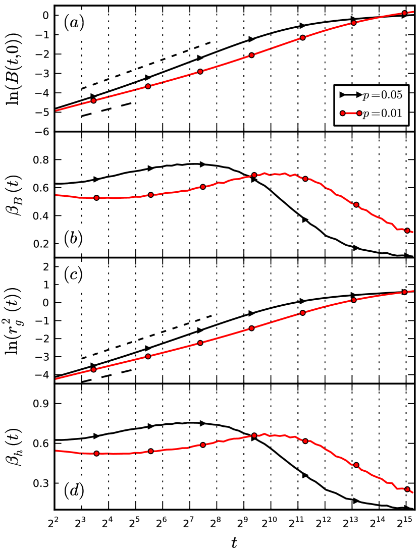
Figure 5: (Color online) Relaxation behavior of (a) the flux line mean-square displacement $B(t,0)$, (c) the squared gyration radius $r_{g}^{2}(t)$, and (b, d) the associated effective exponents $\beta_{B}$ and $\beta_{h}$ over time for non-interacting vortices subject to point pins with potential strength $p=0.01\epsilon_{0}$ ($\bullet$ marker) and $p=0.05\epsilon_{0}$ ($\blacktriangleright$), averaged over $1000$ realizations. For $p=0.01\epsilon_{0}$, the dashed lines (below the curves) indicate the power laws with mean effective exponents $\overline{\beta_{B}}\approx 0.527\pm 0.003$ in (a) and $\overline{\beta_{h}}\approx 0.523\pm 0.002$ in (c) over the range $2^{3}\leq t\leq 2^{5}$. Similarly for $p=0.05\epsilon_{0}$, the dashed lines (above the curves) show the power laws with mean effective exponents $\overline{\beta_{B}}\approx 0.725\pm 0.041$ and $\overline{\beta_{h}}\approx 0.716\pm 0.037$ over the range $2^{3}\leq t\leq 2^{8}$.

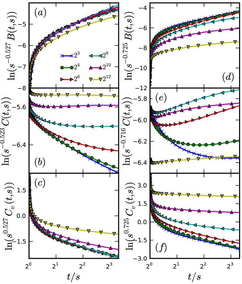
Figure 6: (Color online) Relaxation of (a,d) the mean-square displacement, (b,e) the height autocorrelation function, and (c,f) the density autocorrelation in a system of non-interacting vortex lines of length $L=640$, subject to randomly distributed point pins with a potential depth of (a-c) $p=0.01\epsilon_{0}$ and (d-f) $p=0.05\epsilon_{0}$; data averaged over $1000$ realizations. Time translation invariance is broken throughout the simulation time window. For both pinning strengths, dynamical scaling for the mean-square displacement and the density autocorrelation approximately holds in an intermediate range of waiting times $s$, with the mean effective exponents inferred from Fig. 5.

We now proceed to add point-like disorder with pinning potential strengths $p=0.01\epsilon_{0}$ and $p=0.05\epsilon_{0}$ to a system of non-interacting vortex lines, see Fig. 5. The equilibrium configuration at low temperatures constitutes an extremely dilute vortex glass. For the smaller defect strength of $p=0.01\epsilon_{0}$ there exists an intermediate time regime $2^{3}<t<2^{7}$ during which both effective exponents $\beta_{B}(t)$ and $\beta_{h}(t)$ are fairly constant before developing a maximum around $t=2^{10}$ with a subsequent crossover into a frozen state with $\beta_{B},\beta_{h}\to 0$ where the vortex lines are firmly bound to the point defects [solid lines with black circles in Fig. 5(b,c)]. The slight downward slope at early times is a remnant of the crossover from the random-noise into the EW regime of free flux lines. In fact, the exponent values at times $t<2^{7}$ approximately equal those of the disorder-free system, indicating that the time evolution of the mean lateral vortex position is essentially the same as for free lines prior to the disorder effects becoming noticeable. At later times, vortex movement starts to become affected by the attractive pinning sites, which temporarily accelerates the relaxation kinetics as the vortices are drawn into potential wells, before flux line motion becomes at last frozen at the defects.

Figures 6(a-c) show the resulting relaxation of the two-time mean square displacement $B(t,s)$, the height-height autocorrelation function $C(t,s)$ and the density-density autocorrelation function $C_{v}(t,s)$ for the system with pinning strength $p=0.01\epsilon_{0}$. The global quantities $B$ and $C_{v}$ are scaled using the aging exponent $b=0.527$ taken from the average effective exponent $\beta_{B}$ over the short- to intermediate-time region $2^{3}<t<2^{5}$, where $\beta_{B}$ is roughly constant. These two-time autocorrelation functions yield approximate dynamical scaling for waiting times in this time regime, which further supports the interpretation that pinning sites are essentially irrelevant for the motion of the vortex line mean lateral positions during the early stages of the relaxation process.

In the short-time regime $t<2^{5}$, the squared gyration radius $r_{g}^{2}(t)$ in Fig. 5(c,d) is also described by a power law with an approximate effective exponent $\overline{\beta_{h}}\approx 0.523$. Using this value as the aging exponent for the scaled two-time height-height autocorrelation function $C(t,s)$ in Fig. 6(b) reveals approximate dynamical scaling in this time window. However, stronger deviations from the free-line behavior are observed for $C(t,s)$ than for the other quantities. For larger times $t>2^{6}$ correlations become increasingly longer-lived, since vortex line elements become trapped at pinning sites. Hence, the influence of weak point defects is observed mainly in the fluctuations of flux line elements, whereas the movements of their mean lateral positions are hardly modified.

For a larger pin strength $p=0.05\epsilon_{0}$, the effective exponent maxima in Figs. 5(b,d) develop earlier, near $t=2^{7}$, and there appears no region with approximately constant exponents. For $t>2^{11}$, the system crosses over into a regime where the vortex line configuration appears to become frozen at the pins. This is reflected also in the two-time quantities, where we only see approximate data collapse for $B$ and $C_{v}(t,s)$ for waiting times $s<2^{6}$ [Figs. 6(d,f)]. The two-time height autocorrelation function $C(t,s)$ in Fig. 6(e) yields interesting non-monotonic behavior for $s>2^{3}$, where correlations actually increase again after developing a minimum. We interpret this effect as a rather complicated cross-over effect caused by competition of repulsive, pinning, and elastic forces. Initially, the vortex lines locate nearby pinning sites and are drawn into their attractive potential wells. This yields accelerated super-diffusive motion as indicated by the exponent maximum in Fig. 5(d), until the elastic interaction restricts further exploration of the configuration space and leads to the subsequent decrease of the effective exponent. This behavior is not apparent in the case of $p=0.01$ owing to our choice of waiting times. The exponent maximum in this situation would occur at a much later time and hence the highest waiting time $s=2^{12}$ does not yet display any non-monotonic features.

Elastic manifolds subject to disorder can be characterized by means of the roughness exponent $\chi$ which is defined via the height-height correlation function along the manifold dimensions Nattermann2000 (here, the contour length of the directed lines)

$$C(z-z^{\prime})=\left<[\vec{r}(z)-\vec{r}(z^{\prime})]^{2}\right>\sim|z-z^{\prime}|^{2\chi}\,.$$ (7)

In the case of a dilute flux line system, for which mutual interactions may be neglected, and free of disorder, thermal fluctuations lead to the EW roughness exponent $\chi=0.5$, in agreement with our numerical observations. In the dilute vortex glass phase with point-like disorder, renormalization group analysis of manifolds subject to Gaussian disorder Laessig1998 ; Nattermann2000 predicts a roughness exponent $\chi=5/8$. Our LMD simulations yield a distance-dependent effective roughness exponent in the range of $0.5<\chi_{eff}<0.8$ for a system of non-interacting vortex lines with point-like pinning sites. It should be emphasized, though, that in our model the pinning sites are exclusively attractive. It turns out that the out-of-equilibrium relaxation behavior is considerably different for directed lines subject to a mixture of attractive and repulsive pins: One then actually observes simple aging, albeit with non-universal scaling exponents that depend on temperature as well as pinning strength Iguain2009 ; Pleimling2011 .

4.3 Interacting Vortex Lines without Disorder

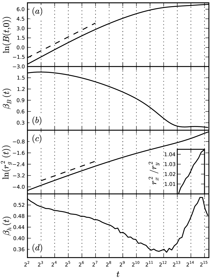
Figure 7: Relaxation behavior of (a) the flux line mean-square displacement $B(t,0)$, (c) the squared gyration radius $r_{g}^{2}(t)$, and (b, d) the associated effective exponents $\beta_{B}$ and $\beta_{h}$ over time for interacting vortices in a system without pinning centers, averaged over $5000$ realizations. The dashed lines indicate power laws with the mean effective exponents (b) $\overline{\beta_{B}}\approx 1.57\pm 0.08$ (averaged over the time range $2^{2}\leq t\leq 2^{6}$) and (d) $\overline{\beta_{h}}\approx 0.50\pm 0.02$ (averaged over $2^{3}\leq t\leq 2^{7}$). The inset in (c) shows the ratio of the $x$ and $y$ components of the radius of gyration for $t>2^{12}$.

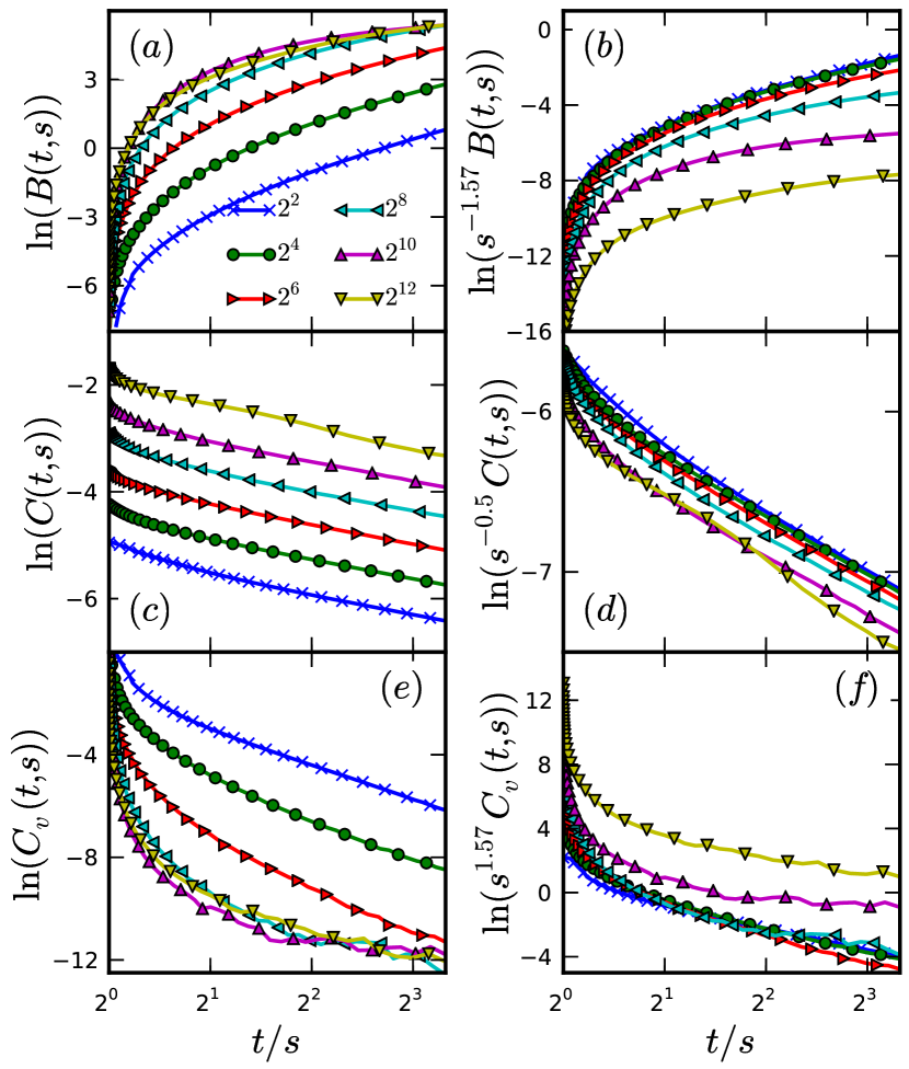
Figure 8: (Color online) Relaxation of (a,d) the mean-square displacement, (b,e) the height autocorrelation function, and (c,f) the density autocorrelation in a system of interacting flux lines without disorder and $L=640$; data averaged over $800$ realizations. The left-hand panels show the unscaled log-log data, whereas data on the right-hand side are scaled by the waiting time $s$ using the mean exponents from Fig. 7.

To disentangle the effects of mutual flux line repulsion from the influence of disordered point pinning sites, we next study the non-equilibrium relaxation of a clean system of interacting vortex lines. Fig. 7 shows the relaxation of the mean-square displacement, the radius of gyration, and the associated effective exponents in this scenario, whereas Fig. 8 displays the behavior of the three two-time autocorrelations. One may immediately identify striking differences between non-interacting and mutually repelling vortex lines in the relaxation of $B(t,s)$ and its associated effective exponent $\beta_{B}(t)$; compare Figs. 3(a,b) and Figs. 7(a,b). The initially large value of $\beta_{B}$ in Fig. 7(b) can be traced to the rapid formation of long-range order due to repulsive vortex interactions. This effect stems from our choice of initial conditions, where the vortex lines are randomly distributed throughout the system. Owing to the initially non-ideal spacing, mutual repulsion leads to fast vortex motion and thus to a large value of $\beta_{B}$. As soon as an optimal arrangement (in this case the Abrikosov lattice) is reached, flux lines perform confined random walks due to the efficient caging from neighboring vortices, which eventually leads to a low effective exponent $\beta_{B}\approx 0.2$ for $t>2^{12}$. The data collapse in Fig. 8(b) shows that an averaged $\overline{\beta_{B}}\approx 1.6$ may serve as the effective aging exponent for the two-time mean square displacement $B(t,s)$ for short waiting times $s<2^{6}$.

The difference between interacting and non-interacting systems does not appear as drastic for the squared radius of gyration $r_{g}^{2}(t)$ as for $B(t,0)$, compare Figs. 3(c,d) and Figs. 7(c,d). After $t>2^{10}$, the Abrikosov lattice starts to form, and the repulsive forces due to neighboring vortex lines increasingly suppress transverse flux line wandering. For $t>2^{12}$, the gyration radius components along the $x$ and $y$ directions assume slightly different values owing to the anisotropic hexagonal vortex line arrangement, which in our rectangular system is always oriented along the $x$ direction; see the inset in Fig. 7(c). For small waiting times $s<2^{6}$, the height autocorrelation data can be collapsed with the EW aging scaling exponent $b=0.5$.

4.4 Interacting Vortex Lines with Point Disorder

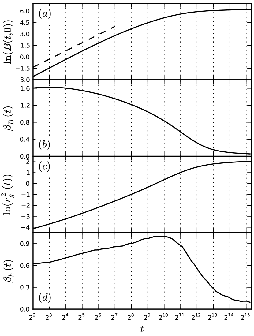
Figure 9: Relaxation behavior of (a) the flux line mean-square displacement $B(t,0)$, (c) the squared gyration radius $r_{g}^{2}(t)$, and (b, d) the associated effective exponents $\beta_{B}$ and $\beta_{h}$ over time for interacting vortices in a system with point-like disorder of strength $p=0.05\epsilon_{0}$, averaged over $1000$ realizations. The dashed line in (a) indicates a power law with the mean effective exponent $\overline{\beta_{B}}\approx 1.54\pm 0.08$ (averaged over the time interval $2^{2}\leq t\leq 2^{7}$).

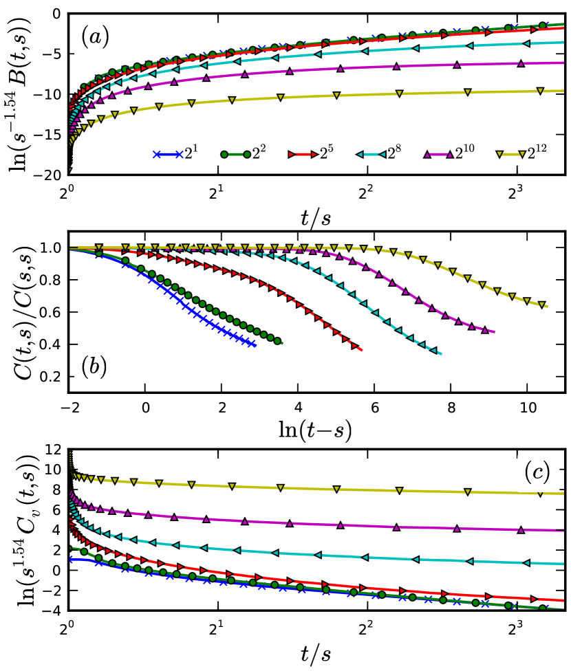
Figure 10: (Color online) Relaxation of (a) the mean-square displacement, (b) the normalized height autocorrelation function, and (c) the density autocorrelation in a system of interacting vortex lines with point pinning centers of strength $p=0.05\epsilon_{0}$ and $L=640$; data averaged over $800$ realizations.

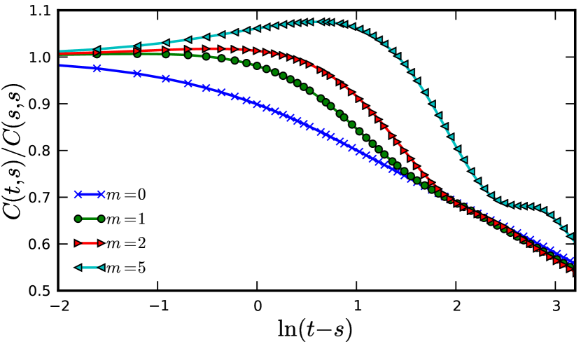
Figure 11: (Color online) The normalized two-time height autocorrelation function $C(t,s)$ for different values of the vortex mass $m$ in a system of interacting flux lines subject to randomly distributed point pins of strength $p=0.05\epsilon_{0}$, at waiting time $s=8$, and averaged over $1000$ simulation runs. The data for $m>0$, for which $C(t,s)$ displays non-monotonic and even oscillatory behavior, was generated using the Brünger-Brooks-Karplus integrator Izaguirre2001 ; Brunger1984 .

We are now in a position to investigate the system of interacting vortex lines subject to attractive point-like disorder. As expected, the global time evolution, see Fig. 9(a,b), which is dictated by the mutual vortex repulsion, is hardly modified by the defects. The effective exponent $\beta_{B}(t)$ displays essentially the same behavior as in the absence of pinning centers; compare Figs. 9(b) and 7(b). Similarly, the aging exponents and the overall shapes of the mean-square displacement and the density-density autocorrelation in Fig. 10(a,c) almost match the simulation results without disorder. For short times $t<2^{6}$, the effective gyration radius exponent $\beta_{h}(t)$ in Fig. 9(d) is quite similar to $\beta_{h}(t)$ in the non-interacting case with point pins, see Fig. 5(d). For longer times, repulsive forces alter the relaxation of $r_{g}^{2}(t)$, which tends towards higher values, Fig. 9(c). Hence, the global observables $B(t,s)$ and $C_{v}(t,s)$ are influenced mainly through the presence or absence of vortex-vortex repulsion through the ensuing mutual caging. The local quantity $C(t,s)$, on the other hand, better probes information on the disorder present in the sample.

In MC simulations Pleimling2011 , an interesting, non-monotonic behavior was revealed in the height-height autocorrelation function for a system of interacting vortex lines subject to point-like disorder: The height autocorrelations displayed a pronounced maximum for small waiting times $s$ and $\ln(t-s)\approx 5$. Yet this feature is absent when the corresponding system is investigated with our LMD algorithm; see Fig. 10(b). In the present study, we have taken the vortex mass per unit length to be small and neglected the inertial term in the Langevin equation; see Sec. 2.2. The algorithm used in Ref. Pleimling2011 assumes a finite displacement per MC step which generates an effective mass. This in turn gives rise to oscillatory behavior at short times. This interpretation is indeed confirmed by LMD simulations that allow for a mass term in the Langevin equation, as depicted in Fig. 11. With increasing vortex mass, $C(t,s)$ shows damped oscillations on top of the monotonic time dependence of the overdamped, zero-mass case.

We observe two-step relaxation behavior, typical e.g. for structural glasses, in the normalized two-time height-height autocorrelation $C(t,s)$ when plotted as a function of the time difference $t-s$, shown in Fig. 10(b). This behavior was also reported in the previous MC study Pleimling2011 : A $\beta$-relaxation regime where $C(t,s)$ is hardly changing and displays time translation invariance precedes the ultimate very slow decay. We attempted to fit a stretched exponential function to our long-time results, but could not achieve satisfactory agreement with our data.

4.5 Non-interacting Vortices with Columnar Defects

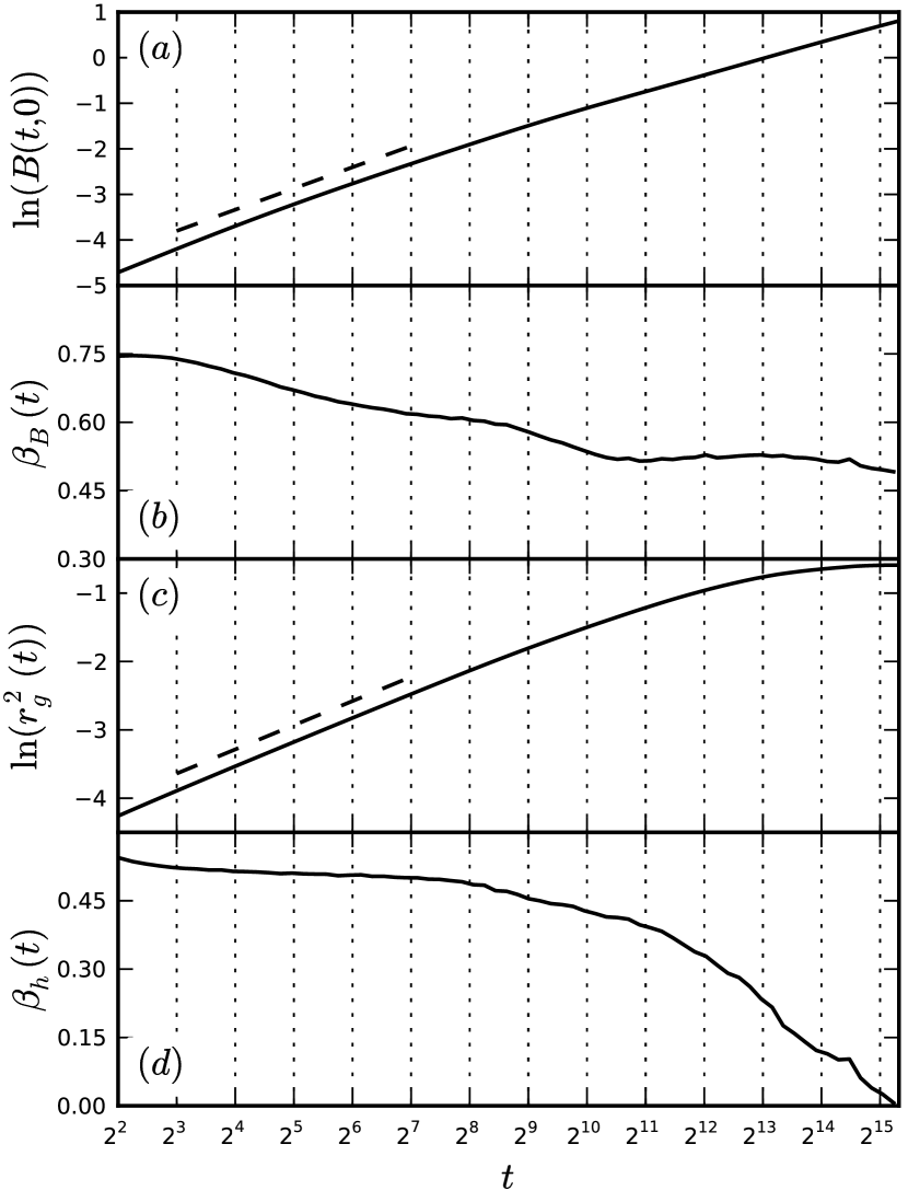
Figure 12: Relaxation behavior of (a) the flux line mean-square displacement $B(t,0)$, (c) the squared gyration radius $r_{g}^{2}(t)$, and (b, d) the associated effective exponents $\beta_{B}$ and $\beta_{h}$ over time for non-interacting vortices subject to columnar pinning centers with $p=0.05\epsilon_{0}$; data averaged over $10000$ realizations. The dashed lines indicate the power laws with the mean effective exponents $\overline{\beta_{B}}\approx 0.672\pm 0.037$ and $\overline{\beta_{h}}\approx 0.510\pm 0.006$ over the time range $2^{3}\leq t\leq 2^{7}$.

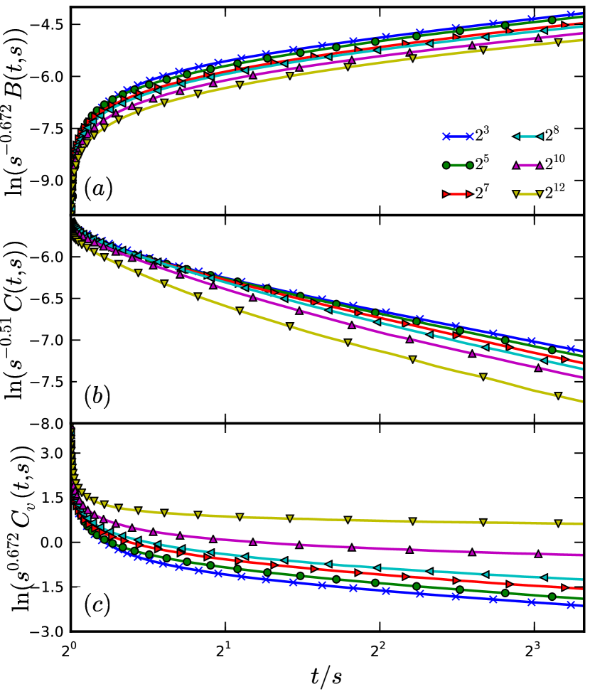
Figure 13: (Color online) Relaxation of (a) the mean-square displacement, (b) the height autocorrelation function, and (c) the density autocorrelation in a system of non-interacting flux lines of length $L=640$ subject to randomly distributed columnar pins of strength $p=0.05\epsilon_{0}$; data averaged over $1000$ realizations. Scaling attempts with the averaged effective exponents taken from Fig. 12 do not yield data collapse for $B(t,s)$ and $C_{v}(t,s)$. One achieves better data collapse at early waiting times $s$ for the height autocorrelations $C(t,s)$.

To compare the effects of uncorrelated point pins with those of extended, correlated defects on the flux line relaxation kinetics, we now investigate a system of non-interacting vortex lines in the presence of columnar pinning centers with a pinning potential strength $p=0.05\epsilon_{0}$. We start by first considering the case of non-interacting flux lines relaxing in the presence of columnar defects. Figure 12 shows the relaxation curves for $B(t,0)$ and $r_{g}^{2}(t)$ with their associated effective exponents $\beta_{B}(t)$ and $\beta_{h}(t)$. The time evolution of the mean-square displacement $B(t,0)$ is slightly accelerated compared to the disorder-free case for times up to $t=2^{9}$; see Fig. 3. This indicates that the initial trapping of vortices at linear pinning sites happens during this time regime. At later times, the effective exponent approaches the value of free flux lines $\beta_{B}=0.5$, due to unbound vortex line wandering. In fact, only $\sim 4$ to $5\%$ of the vortices are pinned at the end of our simulation time window.

As mentioned above, the average number of pinning sites per layer in our simulations is the same for point-like and columnar defects. Hence the combined lateral cross section along the $z$ axis of all pinning sites is much larger for point than it is for columnar pins. Consequently, the probability for a vortex line to encounter a randomly placed columnar pin during what is essentially a random walk is much lower than in samples with randomly placed point defects. A flux line is therefore most likely to be initially captured by a single columnar defect (rather than multiple pinning sites, which would lead to vortex kink configurations) along a short length span, and subsequently becomes completely trapped at that pinning center; this yields rather small values for the final gyration radius, see Figs. 12(c) and 2(b). This is in stark contrast with samples containing uncorrelated point defects, where a single vortex line becomes captured by many pinning sites, which leads to a larger terminal radius of gyration because the line is stretched in random directions between multiple pins; see Sec. 4.2. Thus, point-like pinning centers typically generate rough flux line configurations, whereas columnar defects straighten bound vortices. This fact can be expressed as an effective upward renormalization of the elastic line stiffness, reflected macroscopically as a diverging tilt modulus for the entire vortex system in the pinned Bose glass phase Nelson1993 ; Tauber1997 .

Comparing with the disorder-free system, the time evolution of the effective exponent of the radius of gyration $\beta_{h}(t)$ in the columnar defect case is also different: The exponent initially assumes a value $0.5$ consistent with EW scaling. It begins to deviate from the EW value at $t\approx 2^{9}$, while in the non-disordered case this decrease does not occur until $t\approx 2^{12}$, see Fig. 12(d) and Sec. 4.1. This is due to the fact that thermal line fluctuations inside a single columnar defect are confined to the pinning potential well, which causes early saturation of the equivalent EW growth process. An appreciable number of kinks and double-kinks due to vortices trapped at multiple columnar pinning sites would presumably alter this relaxation behavior, but the occurrence probability of kinks is rather small in our system, as explained above. At low temperatures, our non-interacting flux line system in the presence of correlated disorder forms a very dilute Bose glass, where the number of vortex lines is much less than the number of pinning sites.

Figure 13 shows the relaxation of the three two-time autocorrelation functions for different waiting times $s$ as a function of the ratio $t/s$. We obtain data collapse for the height autocorrelation function $C(t,s)$ when scaling with the appropriately averaged effective aging exponent for early waiting times $s<2^{9}$ and $t/s<2$, which is consistent with the EW regime. The more global mean-square displacement $B(t,s)$ and the density autocorrelation $C_{v}(t,s)$ cannot similarly be scaled to obtain data collapse, because the effective exponent $\beta_{B}(t)$ is never even approximately constant througout the entire observed time interval, as is evident in Fig. 12(b).

4.6 Interacting Vortex Lines with Columnar Defects

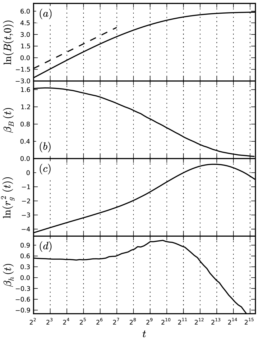
Figure 14: Non-equilibrium relaxation of (a) the flux line mean-square displacement $B(t,0)$, (c) the squared gyration radius $r_{g}^{2}(t)$, and (b, d) the associated effective exponents $\beta_{B}$ and $\beta_{h}$ over time for interacting vortices in a system with columnar defects of strength $p=0.05\epsilon_{0}$, averaged over $1000$ realizations. The dashed line in (a) shows a power law with the mean effective exponent $\overline{\beta_{B}}\approx 1.53\pm 0.11$, averaged over the time interval $2^{2}\leq t\leq 2^{7}$.

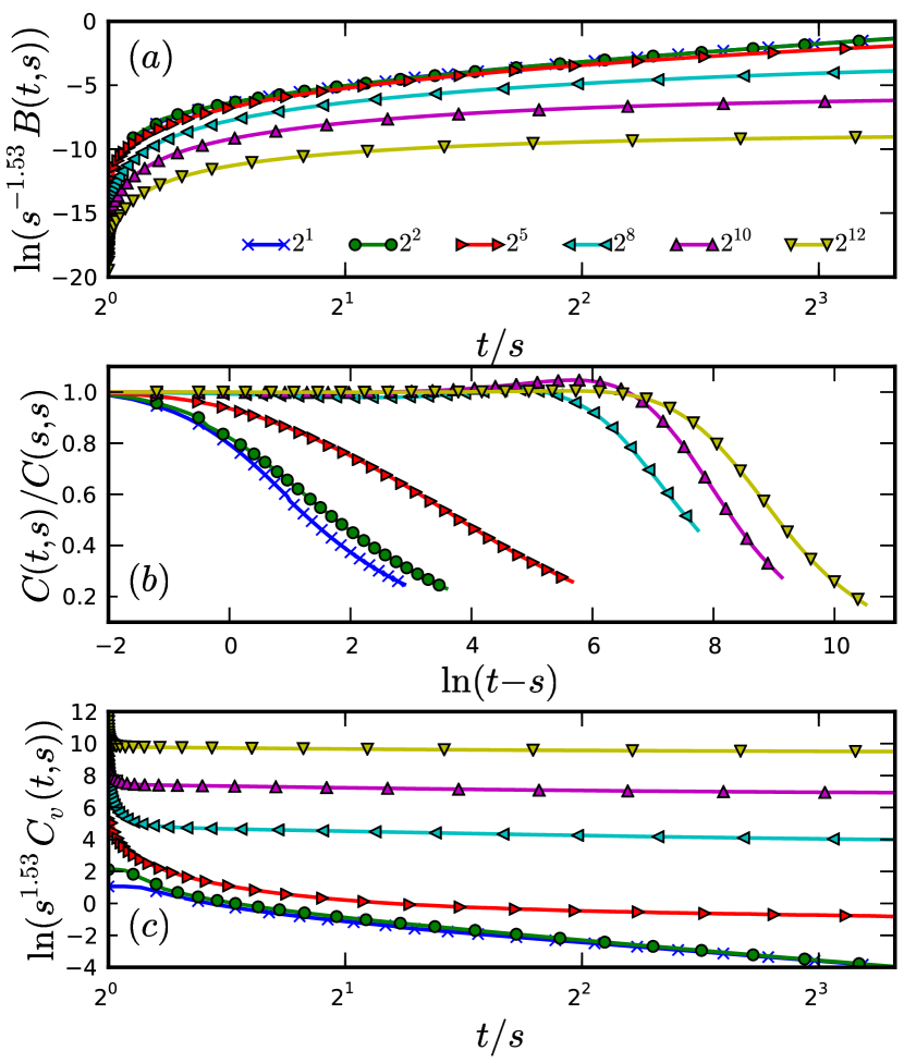
Figure 15: (Color online) Relaxation of (a) the mean-square displacement, (b) the normalized height autocorrelation function, and (c) the density autocorrelation in a system of interacting vortices of length $L=640$ with columnar defects of strength $p=0.05\epsilon_{0}$; data averaged over $800$ realizations.

Next, we again turn on the repulsive vortex-vortex interactions. Similar to the disorder-free system and the samples with point pinning centers, see Secs. 4.3 and 4.4, caging effects accelerate vortex motion, and the shape of the single-time mean-square displacement $B(t,0)$ and its associated effective exponent are hardly modified by the disorder; compare Fig. 14(a,b). At very large times $t>2^{12}$, $B(t,0)$ becomes flatter and approaches a plateau owing to the confinement of vortex lines by attractive defects. This effect is rather more pronounced for columnar pins than for uncorrelated point defects. In fact, the maximal values of $B(t,0)$ and $r_{g}^{2}(t)$ are both smaller in the case of correlated disorder, which indicates tighter binding to the pinning sites.

The radius of gyration also shows similar time evolution trends as compared to samples with point-like disorder; see Figs. 14(c) and 9(c). The effects of attractive columnar pinning sites set in later than for point-like pins, owing to the aforementioned differences in the encounter probability for flux lines and pinning centers. The accelerated growth of the gyration radius for $t>2^{9}$ is due to the pinning at multiple sites and the subsequent formation of kinks, here facilitated by the strong repulsive forces. The non-monotonic behavior of $r_{g}^{2}(t)$ at times $t>2^{13}$ is caused by the decay of previously formed kinks. The density autocorrelation $C_{v}(t,s)$ in Fig. 15(c) becomes flat for waiting times $s>2^{8}$, which supports the interpretation that the vortex lines are essentially trapped by this time and the only remaining relaxation process is the decay of metastable kink configurations.

Figure 15(b) depicts the normalized height-height autocorrelation function of this system for different waiting times $s$. This function shows non-monotonic behavior, but in this situation it cannot stem from an effective mass, as we checked. The appearance of the maximum indicates a fundamental change in the lateral fluctuations. Although we do not yet fully understand this phenomenon, we tentatively relate this observation once again to the decay of kinks in the long-time limit.

4.7 Finite-Size Effects

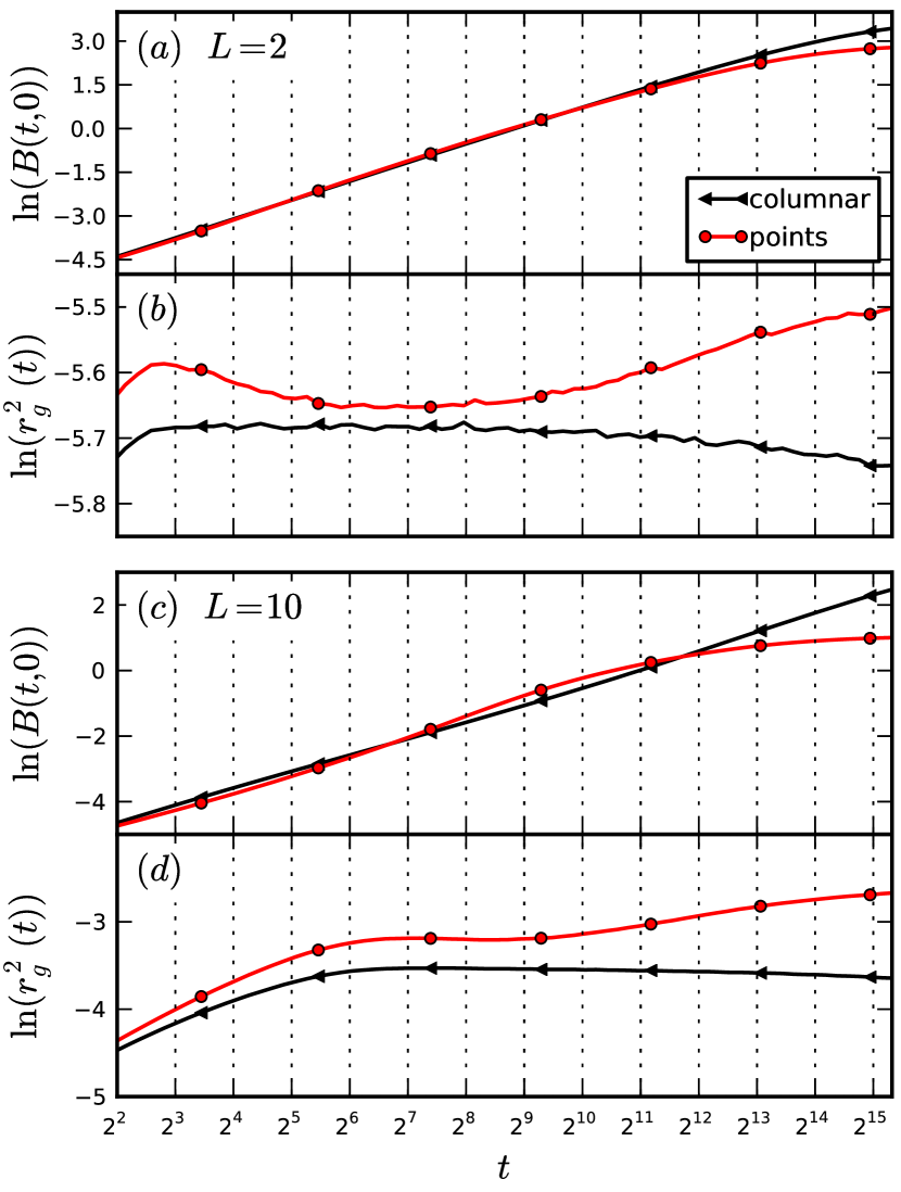
Figure 16: (Color online) Non-equilibrium relaxation of the flux line mean-square displacement $B(t,0)$ and the squared gyration radius $r_{g}^{2}(t)$ over time for non-interacting vortices in systems with point-like and columnar defects with identical pinning strengths $p=0.05\epsilon_{0}$ for (a,b) $L=2$ and (c,d) $L=10$, averaged over $10000$ realizations.

Effects due to the finite flux line length are best analyzed in terms of the second crossover between the EW and saturation regimes for non-interacting vortices in the absence of pinning sites; see Sec. 4.1. (The first crossover between the random thermal noise and the EW regimes only depends on the EW diffusion constant, which here corresponds to the vortex line tension.) The time at which this second crossover occurs depends on the square of the line length, $t_{C}=(L/24b_{0})^{2}2\pi/\epsilon_{0}$ (in the limit of large $L$) Chou2009 . Our choice of $L=640$ for most of the simulation scenarios in this paper thus provides a sufficiently long time window $t_{C}\approx 2^{12}$ to observe the competing effects of vortex interactions and pinning.

Of particular interest is the value of $L$ at which the relaxational difference between point-like and columnar pinning sites becomes apparent. Figure 16 shows a comparison plot of $B(t,0)$ and $r_{g}^{2}(t)$ for both columnar and point-like disorder for very short vortex lines with $L=2$ and $L=10$. In a purely two-dimensional system with $L=1$, where the flux lines are reduced to point particles, there is obviously no difference between the two types of pinning sites. But already for $L=2$ we observe differences in the long-time evolution of $B(t,0)$. The curve for columnar defects can be almost exactly reproduced by using point pins and halving the number of pinning sites. Hence the difference at $L=2$ is largely due to the lower effective density of columnar disorder, as discussed in Sec. 4.5. Yet this equivalence does not extend to the time evolution of the gyration radius $r_{g}^{2}(t)$, which displays small but significant qualitative differences for the two defect types throughout the simulation time window.

For $L=10$, the long-time difference in $B(t,0)$ between columnar and point-like pinning sites can also be explained by the lower effective density of columnar pinning sites. But the deviations appearing at much shorter times reflect genuine physical distinctions in the pinning behavior and ensuing relaxation kinetics.

5 Conclusion

In this paper, we have investigated the differences in the non-equilibrium relaxation features between systems of magnetic flux lines in the presence of point-like and columnar disorder. Proceeding in a systematic way, and considering different limiting cases, allowed us to disentangle the distinct contributions originating from the attractive pinning centers, the repulsive mutual vortex interactions, and the line tension.

We validated both our Langevin Molecular Dynamics simulation code and the Monte Carlo algorithm used in previous studies in a genuine out-of-equilibrium setting by comparing the steady-state vortex velocity and radius of gyration as a function of an external driving force to results from Monte Carlo simulations. As discussed in Sec. 2.7, both these simulation methods need to be tested and validated when applied to non-equilibrium situations. We found that the pinning potential strength in MC is slightly renormalized as compared to LMD due to the (inevitable) choice of a maximal MC step size.

The introduction of columnar instead of point-like pinning sites dramatically changes the steady-state properties. As expected, the critical depinning force is enhanced by approximately an order of magnitude. The radius of gyration is suppressed via vortex line confinement in columnar pinning sites for a driving force well below the critical depinning force. At the transition, partial depinning leads to the formation of half-loops and kinks in the vortex lines and thus to a sharp increase in the radius of gyration. At even higher driving forces, flux line motion is not influenced by pinning.

We carefully studied the relaxation towards equilibrium of a system of initially perfectly straight and randomly-placed vortex lines under various conditions by observing single- and two-time quantities to again compare the effects of uncorrelated point pins and correlated extended defects, and to further validate our LMD code against previously published MC results. We investigated the possibility of data collapse and, hence, a simple aging scenario, by appropriately scaling our two-time quantities. We started with free, non-interacting vortex lines and showed that our results completely agreed with the MC data and the predictions from the Edwards-Wilkinson interface growth model. We then systematically introduced attractive pinning centers and mutual repulsive vortex interactions. Caging effects due to vortex-vortex interactions lead to a considerable acceleration in the relaxation of global quantities, such as the single-time mean-square vortex displacement. A recent study revealed that the MC two-time height-height autocorrelation function for a system with interactions and point-like disorder displayed non-monotonic behavior (shown in Ref. Pleimling2011 ). Comparing with data obtained with an additional inertial term in our LMD algorithm, we argued that these oscillations stem from an effective mass generated by the introduction of a maximal MC step length.

We demonstrated that the relaxation behavior of vortex lines depends crucially on the type of disorder. The vortex and Bose glass phases display complex non-universal relaxation features that are highly dependent on the material parameters. Once a deeper understanding of the transient behavior has been established, detailed information contained in such time-dependent quantities could be used to characterize material properties and specific samples. Point-like disorder binds vortices to many pinning sites at once, while columnar defects capture entire flux lines. When comparing these two defect types, one needs to take into account the difference in the effective pin density and thus the distinct probability of vortex line elements to become trapped. One may characterize the vortex glass phase through the roughness exponent $\chi$ of the spatial height-height correlation function along the strongly fluctuating flux line trajectory. In contrast, correlated linear defects effectively enhance the elastic line stiffness and hence straighten the trapped vortices in the Bose glass phase.

We plan to expand our study to the transient properties of driven vortex lines. The resulting relaxation then is towards a genuine non-equilibrium state in contrast to the relaxation towards equilibrium, which we presented in this paper. Other avenues for further investigations are the study of different and more realistic initial conditions, such as magnetic field or temperature quenches.

References

- (1) D. R. Nelson, Phys. Rev. Lett. 60, 1973 (1988).
- (2) D. R. Nelson and H. S. Seung, Phys. Rev. B 39, 9153 (1989).
- (3) D. R. Nelson, J. Stat. Phys. 57, 511 (1989).
- (4) M. P. A. Fisher, Phys. Rev. Lett. 62, 1415 (1989).
- (5) D. S. Fisher, M. P. A. Fisher, and D. A. Huse, Phys. Rev. B 43, 130 (1991).
- (6) M. V. Feigel’man, V. B. Geshkenbein, A. I. Larkin, and V. M. Vinokur, Phys. Rev. Lett. 63, 2303 (1989).
- (7) T. Nattermann, Phys. Rev. Lett. 64, 2454 (1990).
- (8) G. Blatter, V. B. Geshkenbein, A. I. Larkin, and V. M. Vinokur, Rev. Mod. Phys. 66, 1125 (1994).
- (9) S. S. Banerjee, A. K. Grover, M. J. Higgins, G. I. Menon, P. K. Mishra, D. Pal, S. Ramakrishnan, T. V. Chandrasekhar Rao, G. Ravikumar, V. C. Sahni, S. Sarkar, and C. V. Tomy, Physica C 355, 39 (2001).
- (10) D. R. Nelson and V. M. Vinokur, Phys. Rev. Lett. 68, 2398 (1992).
- (11) I. F. Lyuksyutov, Europhys. Lett. 20, 273 (1992).
- (12) D. R. Nelson and V. M. Vinokur, Phys. Rev. B 48, 13060 (1993).
- (13) M. P. A. Fisher, P. B. Weichman, G. Grinstein, and D. S. Fisher, Phys. Rev. B 40, 546 (1989).
- (14) U. C. Täuber and D. R. Nelson, Phys. Rep. 289, 157 (1997).
- (15) L. C. E. Struik, Physical Aging in Amorphous Polymers and Other Materials (Elsevier, Amsterdam, 1978).
- (16) M. Henkel, M. Pleimling, and E. Sanctuary, eds., Ageing and the Glass Transition, Lecture Notes in Physics 716 (Springer, Berlin, 2007).
- (17) M. Henkel and M. Pleimling, Non-Equilibrium Phase Transitions, Vol.2: Ageing and Dynamical Scaling Far from Equilibrium (Springer, Berlin, 2010).
- (18) L. F. Cugliandolo, in Slow Relaxation and Non Equilibrium Dynamics in Condensed Matter, edited by J.-L. Barrat, J. Dalibart, J. Kurchan, and M. V. Feigel’man (Springer, Berlin, 2003).
- (19) M. Henkel and M. Pleimling, in Rugged Free Energy Landscapes: Common Computational Approaches in Spin Glasses, Structural Glasses and Biological Macromolecules, edited by W. Janke (Springer, Berlin, 2008), Lecture Notes in Physics 736, p. 107.
- (20) X. Du, G. Li, E. Y. Andrei, M. Greenblatt, and P. Shuk, Nat. Phys. 3, 111 (2007).
- (21) M. Nicodemi and H. J. Jensen, Phys. Rev. B 65, 144517 (2002).
- (22) M. Nicodemi and H. J. Jensen, J. Phys. A 34, 8425 (2001).
- (23) H. J. Jensen and M. Nicodemi, Europhys. Lett. 54, 566 (2001).
- (24) M. Nicodemi and H. J. Jensen, Phys. Rev. Lett. 86, 4378 (2001).
- (25) S. Bustingorry, L. F. Cugliandolo, and D. Domínguez, Phys. Rev. Lett. 96, 027001 (2006).
- (26) S. Bustingorry, L. F. Cugliandolo, and D. Domínguez, Phys. Rev. B 75, 024506 (2007).
- (27) L. Civale, A. D. Marwick, T. K. Worthington, M. A. Kirk, J. R. Thompson, L. Krusin-Elbaum, Y. Sun, J. R. Clem, and F. Holtzberg, Phys. Rev. Lett. 67, 648 (1991).
- (28) M. Pleimling and U. C. Täuber, Phys. Rev. B 84, 174509 (2011).
- (29) J. Das, T. J. Bullard, and U. C. Täuber, Physica A 318, 48 (2003).
- (30) T. J. Bullard, J. Das, G. L. Daquila, and U. C. Täuber, Eur. Phys. J. B 65, 469 (2008).
- (31) A. Brass and H. J. Jensen, Phys. Rev. B 39, 9587 (1989).
- (32) M. M. Abdelhadi and K. A. Ziq, Supercond. Sci. Tech. 7, 99 (1994).
- (33) T. Klongcheongsan, T. J. Bullard, and U. C. Täuber, Supercond. Sci. Tech. 23, 025023 (2010).
- (34) V. Gotcheva, A. T. J. Wang, and S. Teitel, Phys. Rev. Lett. 92, 247005 (2004).
- (35) V. Gotcheva, Y. Wang, A. T. J. Wang, and S. Teitel, Phys. Rev. B 72, 064505 (2005).
- (36) M.-B. Luo, and X. Hu, Phys. Rev. Lett. 98, 267002 (2007).
- (37) D. S. Fisher, Phys. Rep. 301, 113 (1998).
- (38) S. F. Edwards and D. R. Wilkinson, Proc. R. Soc. A 381, 17 (1982).
- (39) A. Röthlein, F. Baumann, and M. Pleimling, Phys. Rev. E 76, 019901(E) (2007).
- (40) S. Bustingorry, L. F. Cugliandolo, and J. L. Iguain, J. Stat. Mech. Theor. Exp. 2007, P09008 (2007).
- (41) Y.-L. Chou and M. Pleimling, J. Stat. Mech. Theor. Exp. 2010, P08007 (2010).
- (42) J. A. Izaguirre, D. P. Catarello, J. M. Wozniak, and R. D. Skeel, J. Chem. Phys. 114, 2090 (2001).
- (43) A. Brünger, C. L. Brooks, and M. Karplus, Chem. Phys. Lett. 105, 495 (1984).
- (44) Y.-L. Chou, M. Pleimling, and R. K. P. Zia, Phys. Rev. E 80, 061602 (2009).
- (45) T. Nattermann and S. Scheidl, Adv. Phys. 49, 607 (2000).
- (46) M. Lässig, Phys. Rev. Lett. 80, 2366 (1998).
- (47) J. L. Iguain, S. Bustingorry, A. B. Kolton, and L. F. Cugliandolo, Phys. Rev. B 80, 094201 (2009).