On generalized multinomial models and joint percentile estimation

Abstract

This article proposes a family of link functions for the multinomial response model. The link family includes the multicategorical logistic link as one of its members. Conditions for the local orthogonality of the link and the regression parameters are given. It is shown that local orthogonality of the parameters in a neighbourhood makes the link family location and scale invariant. Confidence regions for jointly estimating the percentiles based on the parametric family of link functions are also determined. A numerical example based on a combination drug study is used to illustrate the proposed parametric link family and the confidence regions for joint percentile estimation.

Keywords: confidence regions, multicategorical logistic link, parameter orthogonality, standardization

1 Introduction

In this article we address two issues related to multinomial response models, (i) a family of link functions and (ii) percentile estimation under a parametric link family. In the first few sections we propose a family of link functions for multinomial nominal response models. When working with multinomial data sets the common practice is to fit the multicategory logistic link function (Agresti, 2002, pp. 267-274). However, Czado and Santner (1992) show that if the link function is incorrectly assumed then it leads to biased estimates thus increasing the mean squared error of prediction. Using a data set based on a combination drug therapy experiment we show that parameter estimation is improved by using the proposed link family instead of the commonly used multivariate logistic link. The parametric link family proposed includes the multivariate logistic link as one of its members. In the later part of the article we discuss three methods for finding confidence regions for the percentiles of a multinomial response model. The confidence regions determined are based on the estimated values of the link parameters.

In univariate generalized linear models (GLMs), especially for binary data, family of link functions have been discussed by many researchers. Some of the one and two parameter link families for binary models are, proposed by namely Prentice (1975, 1976); Pregibon (1980); Guerrero and Johnson (1982); Aranda-Ordaz (1981); Stukel (1988); Czado and Santner (1992); Czado (1992, 1993, 1997); Lang (1999). However, unlike binary regression models research papers on link families for multinomial responses are rarely found in the literature. The two parametric link families proposed by Genter and Farewell (1985) and Lang (1999) are only applicable to multinomial data sets with ordered categories. Till date we were unable to find any work which addresses a family of link functions for multinomial data sets with nominal responses. The situation is similar for percentile estimation methods in multinomial response models. Though a huge number of research papers (namely, Hamilton (1979); Carter et al. (1986); Williams (1986); Huang (2001); Biedermann et al. (2006); Li and Wiens (2011)) have been written on percentile estimation and effect of link misspecification on percentile estimation for binary data, almost no work has been done in the case of multinomial data. There are, however, many experimental situations where multinomial responses may be observed for each setting of a group of control variables. As a typical example we may consider a drug testing experiment, where both the efficacious and toxic responses of the drug/s are measured on the subjects. This results in two responses, efficacy and toxicity of the drug, both of which are binary in nature. Since the responses come from the same subject they are assumed to be correlated, and can be modeled using a multinomial distribution (Mukhopadhyay and Khuri, 2008). In this situation it may be of interest to the experimenter to jointly estimate the $100p$ percentile of the efficacy and toxic responses. In this article we discuss a numerical example based on the pain relieving and toxic effects of two analgesic drugs and determine confidence regions for the $100$p percentiles of both the responses.

While parametric link families are able to improve the maximum likelihood fit when compared to canonical links, any correlation between the link and the regression parameters leads to an increase in the variances of the parameter estimates [Czado (1997)]. However, it can be shown that if the parameters are orthogonal to each other then the variance inflation reduces to zero for large sample sizes (Cox and Reid, 1987). Conditions for local orthogonality in a neighbourhood was proposed by Czado (1997) for univariate GLMs. In this article we extend these conditions so that we can apply them to a multiresponse situation. It is also shown that the local orthogonality of the parameters imply location and scale invariance of the family of link functions.

The remainder of the article is organized as follows: In Section 2 we describe the family of link functions for the multinomial model. Detailed conditions of local orthogonality between the link and the regression parameters are given in Section 3. In Section 4 we discuss three interval methods for percentile estimation in a multinomial model. The proposed link family and confidence regions are illustrated with a numerical example based on a drug testing experiment in Section 5. Concluding remarks are given in Section 6.

2 A family of link functions for multinomial data

In this section the multinomial response model with a parametric link function is introduced. We use a scaled version of the multinomial distribution. The following three components are used to describe it:

• Distributional component: A random sample of size $n$, $\mathbb{y}_{1},\ldots,\mathbb{y}_{n}$, is selected from a multinomial distribution with parameters $(\boldsymbol{\pi}_{i},n_{i});\,\boldsymbol{\pi}_{i}=(\pi_{i1},\ldots,\pi_{iq}),\,i=1,\ldots,n$. The density function of $\bar{\textbf{y}}_{i}={\textbf{y}}_{i}/n_{i}$ also called the scaled multinomial distribution (Fahrmeir and Tutz, 2001, p 76) is,

  $$s(\bar{\textbf{y}}_{i}|\boldsymbol{\theta}_{i},\phi,\omega)=\exp\left\{\frac{[\bar{\textbf{y}}^{\prime}_{i}\boldsymbol{\theta}_{i}-b(\boldsymbol{\theta}_{i})]}{\phi}\omega_{i}+c(\textbf{y}_{i},\phi,\omega_{i})\right\},$$ (2.1)

  where $\boldsymbol{\theta}_{i}=\left[\log(\frac{\pi_{i1}}{1-\sum_{j=1}^{q}\pi_{ij}}),\ldots,\log(\frac{\pi_{iq}}{1-\sum_{j=1}^{q}\pi_{ij}})\right]^{\prime}$, $b(\boldsymbol{\theta}_{i})=-\log({1-\sum_{j=1}^{q}\pi_{ij}})$, $c({\textbf{y}}_{i},\phi,\omega_{i})=\log\left(\frac{n_{i}!}{y_{i1}!\ldots y_{iq}!(n_{i}-y_{i1}-\ldots-y_{iq})!}\right)$, $\omega_{i}=n_{i}$ and $\phi=1$. The total number of observations is $N=\sum_{i=1}^{n}n_{i}$.

• Linear predictor: A $q$ dimensional linear predictor, $\boldsymbol{\eta}(\mathbf{x})=\mathbf{Z}(\mathbf{x})\boldsymbol{\beta}$, where $\mathbf{Z}(\mathbf{x})=\bigoplus_{j=1}^{q}\textbf{f}_{j}(\textbf{x})$, $\textbf{f}_{j}(\textbf{x})$ is a known vector function of x, $\boldsymbol{\beta}=[\boldsymbol{\beta}_{1}^{\prime},\ldots,\boldsymbol{\beta}_{q}^{\prime}]^{\prime}$ is the $p\times 1$ vector of unknown parameters with the $j$th component, $\boldsymbol{\beta}_{j}$, of length $p_{j}$ and $p=\sum_{j=1}^{q}p_{j}$.

• Parametric link function: $\boldsymbol{\mu}=\boldsymbol{\pi}=\mathbf{h}(\boldsymbol{\alpha},\boldsymbol{\eta})$, where $\mathbf{h}(\boldsymbol{\alpha},\cdot)=[h_{1}(\boldsymbol{\alpha},\cdot),\ldots,h_{q}(\boldsymbol{\alpha},\cdot)]^{\prime}$, $\boldsymbol{\alpha}_{r\times 1}=[\boldsymbol{\alpha}_{1}^{\prime},\ldots,\boldsymbol{\alpha}_{q}^{\prime}]^{\prime}$, $\boldsymbol{\alpha}_{j}$ is of length $r_{j}$ and $\sum_{j=1}^{q}r_{j}=r$.

2.1 Proposed form of parametric link function

Several researchers (Stukel, 1988; Czado, 1989) propose the following generalization for binary response models with a logistic link function

$$\mu(\mathbf{x})=E(y|\mathbf{x})=h(\boldsymbol{\alpha},\eta)=\frac{\exp\{G(\boldsymbol{\alpha},\eta)\}}{[1+\exp\{G(\boldsymbol{\alpha},\eta)\}]},$$

where $G(\boldsymbol{\alpha},\cdot)$ is a generating family with the unknown link parameter $\boldsymbol{\alpha}$. For example using the generating family by Czado (1989) we get

$$G(\boldsymbol{\alpha},\eta)=\left\{\begin{matrix}\frac{(1+\eta)^{\alpha_{1}}-1}{\alpha_{1}}&\text{if}&\eta\geq 0\\ -\frac{(1-\eta)^{\alpha_{2}}-1}{\alpha_{2}}&\text{if}&\eta<0,\end{matrix}\right.$$

where $\boldsymbol{\alpha}=[\alpha_{1},\alpha_{2}]^{\prime}$. Usually when modeling the mean in a multinomial response model the multivariate version of the logit model (Agresti, 2002, pp. 267-274) is used,

$$\pi_{j}=h_{j}(\boldsymbol{\eta})=\frac{\exp(\eta_{j})}{1+\sum_{l=1}^{q}\exp(\eta_{l})},\text{ for $j=1,\ldots,q$}.$$

An alternative form of the above model is given by using the link function $\mathbf{g}$ where $\mathbf{g}=\mathbf{h}^{-1}$,

$$\eta_{j}=g_{j}(\boldsymbol{\mu})=\log\frac{\mu_{j}}{1-\sum_{j=1}^{q}\mu_{j}}.$$

Analogous to the binary case we propose the following generalization of the multicategorical logit model,

$$\pi_{j}=h_{j}(\boldsymbol{\alpha},\boldsymbol{\eta})=\frac{\exp\{G_{j}(\boldsymbol{\alpha}_{j},\eta_{j})\}}{1+\sum_{l=1}^{q}\exp\{G_{l}(\boldsymbol{\alpha}_{l},\eta_{l})\}},\text{ for $j=1,\ldots,q$},$$ (2.2)

where $\mathbf{G}=[G_{1},G_{2},\ldots,G_{q}]^{\prime}$, $G_{j}(\boldsymbol{\alpha}_{j},\cdot)$ is a generating family for binary response models as described above, $h_{j}(\boldsymbol{\alpha},\cdot)$ is the $j$th component of $\mathbf{h}(\boldsymbol{\alpha},\cdot)=\mathbf{g}^{-1}(\boldsymbol{\alpha},\cdot)$. The family $\Lambda=\{\mathbf{h}(\boldsymbol{\alpha},\cdot):\boldsymbol{\alpha}\in\boldsymbol{\Omega}\}$ includes the multivariate logistic link function if there exists an $\boldsymbol{\alpha}_{0}\in\boldsymbol{\Omega}$ such that $\mathbf{G}(\boldsymbol{\alpha}_{0},\cdot)$ is a identity function.

2.2 Parameter estimation

Summing up the previous sections we can write the multinomial model with a parametric link function as,

$$\boldsymbol{\pi}(\mathbf{x})=\mathbf{h}[\boldsymbol{\alpha},\boldsymbol{\eta}(\mathbf{x})],$$ (2.3)

where $\boldsymbol{\eta}(\mathbf{x})=[\boldsymbol{\eta}_{1}(\mathbf{x}),\ldots,\boldsymbol{\eta}_{q}(\mathbf{x})]^{\prime}=\mathbf{Z}(\mathbf{x})\boldsymbol{\beta},\,\mathbf{x}\in R^{k}$, $\boldsymbol{\beta}$ is a $p\times 1$ vector of unknown parameters and $\boldsymbol{\alpha}$ is $r\times 1$ vector of unknown link parameters. Also,

$$\boldsymbol{\eta}_{j}=\boldsymbol{\eta}_{j}(\mathbf{x})=\mathbf{f}_{j}(\mathbf{x})\boldsymbol{\beta}_{j}=\mathbf{g}_{j}[\boldsymbol{\alpha},\boldsymbol{\pi}(\mathbf{x})],\text{ for $j=1,\ldots,q$},$$ (2.4)

where $\mathbf{g}=[\mathbf{g}_{1},\ldots,\mathbf{g}_{q}]^{\prime}$ is the inverse of $\mathbf{h}=[\mathbf{h}_{1},\ldots,\mathbf{h}_{q}]^{\prime}$. We use the notation $\boldsymbol{\delta}$ to denote the joint vector of the regression and link parameters, thus $\boldsymbol{\delta}=[\boldsymbol{\beta}^{\prime},\boldsymbol{\alpha}^{\prime}]^{\prime}$ is a vector of length $(p+r)$. The parameter vector $\boldsymbol{\delta}$ is estimated using the maximum likelihood estimation (MLE) method. A brief description of the procedure is given as follows:

Using the scaled version of the multinomial distribution as described in equation (2.1) the log-likelihood function for the sample $\mathbf{y}_{1},\ldots,\mathbf{y}_{n}$ is,

$$l(\boldsymbol{\delta}) = \sum_{i=1}^{n}l_{i}(\boldsymbol{\delta})$$ (2.5)

$$= \sum_{i=1}^{n}[\bar{\mathbf{y}}_{i}^{\prime}\boldsymbol{\theta}_{i}-b(\boldsymbol{\theta}_{i})]n_{i}+constant.$$

Thus the score function is (Fahrmeir and Tutz, 2001, p 436),

$$\frac{\partial l(\boldsymbol{\delta})}{\partial\boldsymbol{\delta}} = \frac{\partial}{\partial\boldsymbol{\delta}}\sum_{i=1}^{n}[\bar{\mathbf{y}}_{i}^{\prime}\boldsymbol{\theta}_{i}-b(\boldsymbol{\theta}_{i})]n_{i}$$ (2.6)

$$= \sum_{i=1}^{n}\frac{\partial\boldsymbol{\mu}_{i}}{\partial\boldsymbol{\delta}}[Var(\bar{\mathbf{y}}_{i})]^{-1}(\bar{\mathbf{y}}_{i}-\boldsymbol{\mu}_{i}),$$

and (Fahrmeir and Tutz, 2001, p 436)

$$-\frac{\partial^{2}l(\boldsymbol{\delta})}{\partial\boldsymbol{\delta}\partial\boldsymbol{\delta}^{\prime}} = \sum_{i=1}^{n}\frac{\partial\boldsymbol{\mu}_{i}}{\partial\boldsymbol{\delta}}[Var(\bar{\mathbf{y}}_{i})]^{-1}\frac{\partial\boldsymbol{\mu}_{i}}{\partial\boldsymbol{\delta}^{\prime}}-\sum_{i=1}^{n}\sum_{j=1}^{q}\frac{\partial^{2}\theta_{ij}}{\partial\boldsymbol{\delta}\partial\boldsymbol{\delta}^{\prime}}(\bar{y}_{ij}-\mu_{ij})n_{i}$$ (2.7)

$$= \mathbf{H}_{n},\ (say).$$

From equation (2.7) we get the Fisher information matrix to be

$$\mathbf{J}_{n} = -E\left[\frac{\partial^{2}l(\boldsymbol{\delta})}{\partial\boldsymbol{\delta}\partial\boldsymbol{\delta}^{\prime}}\right]=\sum_{i=1}^{n}\frac{\partial\boldsymbol{\mu}_{i}}{\partial\boldsymbol{\delta}}[Var(\bar{\mathbf{y}}_{i})]^{-1}\frac{\partial\boldsymbol{\mu}_{i}}{\partial\boldsymbol{\delta}^{\prime}}.$$ (2.8)

For maximizing the log-likelihood the Fisher scoring iteration method is used which yields,

$$\boldsymbol{\delta}^{(m+1)}=\boldsymbol{\delta}^{(m)}+\mathbf{J}_{n}^{-1}\frac{\partial l[\boldsymbol{\delta}^{(m)}]}{\partial\boldsymbol{\delta}},$$ (2.9)

where $m$ indicates the $m$th iteration. It is also possible to use the method given in Stukel (1988) for finding an approximate MLE of $\boldsymbol{\delta}$. In this method, the MLE of $\boldsymbol{\beta}$ is obtained by fixing $\boldsymbol{\alpha}$ and denoted by $\hat{\beta}(\boldsymbol{\alpha})$. An approximate MLE of $\boldsymbol{\delta}$ is then given by $\hat{\boldsymbol{\delta}}=[\hat{\boldsymbol{\beta}}^{\prime}(\hat{\boldsymbol{\alpha}}),\hat{\boldsymbol{\alpha}}^{\prime}]^{\prime}$ which maximizes the log-likelihood function over a set $\boldsymbol{\alpha}$.

2.3 Asymptotic distribution of $\hat{\boldsymbol{\delta}}$

Suppose $\hat{\boldsymbol{\delta}}=[\hat{\boldsymbol{\beta}}^{\prime},\hat{\boldsymbol{\alpha}}^{\prime}]^{\prime}$ denotes the MLE of $\boldsymbol{\delta}$. Using equation (2.6) and the central limit theorem we know $\frac{\partial l(\boldsymbol{\delta})}{\partial\boldsymbol{\delta}}$ asymptotically follows a normal distribution with mean $\mathbf{0}$ and variance $\mathbf{J}_{n}$. By first order Taylor series expansion,

$$\mathbf{0}=\frac{\partial l(\hat{\boldsymbol{\delta}})}{\partial\boldsymbol{\delta}} = \frac{\partial l(\boldsymbol{\delta})}{\partial\boldsymbol{\delta}}+\left[\frac{\partial^{2}l(\boldsymbol{\delta})}{\partial\boldsymbol{\delta}\partial\boldsymbol{\delta}^{\prime}}\right](\hat{\boldsymbol{\delta}}-\boldsymbol{\delta}).$$

This implies (Fahrmeir and Tutz, 2001, p 439),

$$\sqrt{N}(\hat{\boldsymbol{\delta}}-\boldsymbol{\delta}) = \sqrt{N}\mathbf{H}^{-1}_{n}\frac{\partial l(\boldsymbol{\delta})}{\partial\boldsymbol{\delta}}=\sqrt{N}\mathbf{J}_{n}^{-1}\frac{\partial l(\boldsymbol{\delta})}{\partial\boldsymbol{\delta}}+O_{p}(N^{-1/2}).$$

Thus, we get that $\hat{\boldsymbol{\delta}}$ has an asymptotic normal distribution with mean $\boldsymbol{\delta}$ and variance $\mathbf{J}_{n}^{-1}$.

3 Orthogonalization of link and regression parameter vectors

In this section we discuss certain conditions for which the link parameters are approximately orthogonal to the regression parameters in a neighbourhood asymptotically. In our numerical examples we show that approximate orthogonality of the parameters reduces the variance inflation of $\hat{\boldsymbol{\beta}}$ while increasing the numerical stability of the computations. The family of link functions for which the regression parameters are approximately orthogonal to the link parameters in a neighbourhood are also location and scale invariant. Li and Duan (1989) noted the importance of a family of link function being location and scale invariant. In their paper they observed that for a unspecified link function the intercept parameter was not identified while the slope parameter was identified only up to a multiplicative constant. Thus any variation in the location and scale was absorbed by the link function.

Proposition 1: The regression parameter vector $\boldsymbol{\beta}$ and link parameter vector $\boldsymbol{\alpha}$ are approximately orthogonal in a neighbourhood around $\boldsymbol{\eta}_{0}$, if the family of link functions $\mathbf{h}(\boldsymbol{\alpha},\cdot)$ satisfies the following conditions, (i) there exists $\boldsymbol{\eta}_{0}$ and $\boldsymbol{\pi}_{0}$ such that

$$\mathbf{h}(\boldsymbol{\alpha},\boldsymbol{\eta}_{0})=\boldsymbol{\pi}_{0},\ \forall\ \boldsymbol{\alpha}\in\Omega,$$ (3.1)

and (ii) there exists a $\mathbf{s}_{0}$ such that

$$\frac{\partial\mathbf{h}(\boldsymbol{\alpha},\boldsymbol{\eta})}{\partial\boldsymbol{\eta}}\left|{}_{\boldsymbol{\eta}=\boldsymbol{\eta}_{0}}\right.=\mathbf{s}_{0},\ \forall\ \boldsymbol{\alpha}\in\Omega.$$ (3.2)

Proof: By first order Taylor series expansion of $\mathbf{h}(\boldsymbol{\alpha},\boldsymbol{\eta})$ around $\boldsymbol{\eta}_{0}$ and equations (3.1) and (3.2),

$$\mathbf{h}(\boldsymbol{\alpha},\boldsymbol{\eta}) \approx \mathbf{h}(\boldsymbol{\alpha},\boldsymbol{\eta}_{0})+\frac{\partial\mathbf{h}(\boldsymbol{\alpha},\boldsymbol{\eta})}{\partial\boldsymbol{\eta}}\left|{}_{\boldsymbol{\eta}=\boldsymbol{\eta}_{0}}\right.(\boldsymbol{\eta}-\boldsymbol{\eta}_{0})$$ (3.3)

$$= \boldsymbol{\pi}_{0}+\mathbf{s}_{0}(\boldsymbol{\eta}-\boldsymbol{\eta}_{0}).$$ (3.4)

Equation (3.4) shows that the family of link functions $\mathbf{h}(\boldsymbol{\alpha},\cdot)$ is approximately independent of $\boldsymbol{\alpha}$ in a neighbourhood of $\boldsymbol{\eta}_{0}$ where approximation (3.3) holds asymptotically. Hence, if the conditions (3.1) and (3.2) are satisfied, then the regression parameters $\boldsymbol{\beta}$ and the link parameters $\boldsymbol{\alpha}$ are approximately orthogonal in a neighbourhood of $\boldsymbol{\eta}_{0}$ asymptotically.

Extending the definition of a location and scale invariant family given by Czado (1997) to the multiple response case we state: a family $\boldsymbol{\Lambda}$ is said to be location and scale invariant if for every $\mathbf{h}\in\boldsymbol{\Lambda}$, the function $\mathbf{h}^{*}(\boldsymbol{\alpha},\boldsymbol{\eta})=\mathbf{h}(\boldsymbol{\alpha},\mathbf{a}+\mathbf{b}\boldsymbol{\eta})\notin\boldsymbol{\Lambda}$ for all $\mathbf{a}\neq\mathbf{0}_{a}$ and $\mathbf{b}\neq\mathbf{0}_{b}$ or $\mathbf{I}_{b}$, where $\mathbf{a}=[a_{1},\ldots,a_{q}]^{\prime}$, $\mathbf{b}=diag(b_{1},\ldots,b_{q})$, $\mathbf{0}_{a}$ is a matrix of the same order as $\mathbf{a}$ with all elements zero, $\mathbf{0}_{b}$ is a matrix of same order as $\mathbf{b}$ with all elements zero and $\mathbf{I}_{b}$ is an identity matrix with the same order as $\mathbf{b}$.

Proposition 2: If every member of a family $\boldsymbol{\Lambda}=\{\mathbf{h}(\boldsymbol{\alpha},\cdot):\boldsymbol{\alpha}\in\boldsymbol{\Omega}\}$ satisfies conditions (3.1) and (3.2) for fixed $\boldsymbol{\pi}_{0}$ and $\mathbf{s}_{0}$, then $\boldsymbol{\Lambda}$ is location and scale invariant.

Proof: Suppose every member $\mathbf{h}$ of the family $\boldsymbol{\Lambda}$ satisfies conditions (3.1) and (3.2) for fixed $\boldsymbol{\pi}_{0}$ and $\mathbf{s}_{0}$. Define $\mathbf{h}^{*}(\boldsymbol{\alpha},\boldsymbol{\eta})=\mathbf{h}(\boldsymbol{\alpha},\mathbf{a}+\mathbf{b}\boldsymbol{\eta})$, then at $\boldsymbol{\eta}^{*}=\mathbf{b}^{-1}(\boldsymbol{\eta}_{0}-\mathbf{a})$,

$$\mathbf{h}^{*}(\boldsymbol{\alpha},\boldsymbol{\eta}^{*})=\mathbf{h}(\boldsymbol{\alpha},\boldsymbol{\eta}_{0})=\boldsymbol{\pi}_{0}\ \forall\ \boldsymbol{\alpha}\ \in\boldsymbol{\Omega},$$

where $\mathbf{a}\neq\mathbf{0}_{a}$ and $\mathbf{b}\neq\mathbf{0}_{b}$ or $\mathbf{I}_{b}$. Thus, equation (3.1) is satisfied by $\mathbf{h}^{*}$ at $\boldsymbol{\eta}=\boldsymbol{\eta}^{*}$. Also,

$$\frac{\partial\mathbf{h}^{*}(\boldsymbol{\alpha},\boldsymbol{\eta})}{\partial\boldsymbol{\eta}}|_{\boldsymbol{\eta}=\boldsymbol{\eta}^{*}} = \frac{\partial\mathbf{h}(\boldsymbol{\alpha},\mathbf{a}+\mathbf{b}\boldsymbol{\eta})}{\partial\boldsymbol{\eta}}|_{\boldsymbol{\eta}=\boldsymbol{\eta}^{*}}=\mathbf{b}\frac{\partial\mathbf{h}(\boldsymbol{\alpha},\boldsymbol{\eta})}{\partial\boldsymbol{\eta}}|_{\boldsymbol{\eta}=\boldsymbol{\eta}_{0}}=\mathbf{b}\mathbf{s}_{0}\neq\mathbf{s}_{0},$$

for $\mathbf{b}\neq\mathbf{I}_{b}$, implying $\mathbf{h}^{*}\notin\boldsymbol{\Lambda}$ for $\mathbf{a}\neq\mathbf{0}_{a}$ and $\mathbf{b}\neq\mathbf{0}_{b}$ or $\mathbf{I}_{b}$. Hence the family $\boldsymbol{\Lambda}$ is location and scale invariant.

3.1 Construction of $(\boldsymbol{\pi}_{0},\mathbf{s}_{0})$-standardized link families at $\boldsymbol{\eta}_{0}$

A family $\boldsymbol{\Lambda}$ satisfying conditions (3.1) and (3.2) is called $(\boldsymbol{\pi}_{0},\mathbf{s}_{0})$-standardized at $\boldsymbol{\eta}_{0}$ (Czado, 1997).

Proposition 3: Suppose $\mathbf{G}(\boldsymbol{\alpha},\boldsymbol{\eta})=[G_{1}(\boldsymbol{\alpha}_{1},\eta_{1}),\ldots,G_{q}(\boldsymbol{\alpha}_{q},\eta_{q})]^{\prime}$ where $\boldsymbol{\alpha}=[\boldsymbol{\alpha}_{1},\ldots,\boldsymbol{\alpha}_{q}]^{\prime}$ and $\boldsymbol{\eta}=[\eta_{1},\ldots,\eta_{q}]^{\prime}$, such that each {$G_{j}(\boldsymbol{\alpha}_{j},\eta_{j}),\ \boldsymbol{\alpha}_{j}\in\Omega_{j}$} is a generating family for binary response models and are $(\mu_{0j},s_{0j})$-standardized at $\eta_{0j}$ for $j=1,2,\ldots,q$. Then the family $\boldsymbol{\Lambda}_{\mathbf{g}}=\{\mathbf{G}(\boldsymbol{\alpha},\cdot):\boldsymbol{\alpha}\in\boldsymbol{\Omega}=\Omega_{1}\times\ldots\times\Omega_{q}$} is $(\boldsymbol{\pi}_{0},\mathbf{s}_{0})$-standardized at $\boldsymbol{\eta}_{0}$, where $\boldsymbol{\eta}_{0}=[\eta_{01},\ldots,\eta_{0q}]^{\prime}$, $\boldsymbol{\pi}_{0}=[\mu_{01},\ldots,\mu_{0q}]^{\prime}$, and $\mathbf{s}_{0}=diag\{s_{01},\ldots,s_{0q}\}$.

Proof: Since, $G_{j}(\boldsymbol{\alpha}_{j},\eta_{j})$ is $(\mu_{0j},s_{0j})$-standardized at $\eta_{0j}$, $G_{j}(\boldsymbol{\alpha}_{j},\eta_{0j})=\mu_{0j},\ \forall\ \boldsymbol{\alpha}_{j}\in\Omega_{j},$ and $\frac{\partial G_{j}(\boldsymbol{\alpha},\eta)}{\partial\eta}|_{\eta=\eta_{0j}}=s_{0j},\ \forall\ \boldsymbol{\alpha}_{j}\in\Omega_{j}$. Thus, $\mathbf{G}(\boldsymbol{\alpha},\boldsymbol{\eta}_{0})=[\mu_{01},\mu_{02},\ldots,\mu_{0q}]^{\prime}=\boldsymbol{\pi}_{0},\ \forall\ \boldsymbol{\alpha}\in\boldsymbol{\Omega}$, and $\frac{\partial\mathbf{G}(\boldsymbol{\alpha},\boldsymbol{\eta})}{\partial\boldsymbol{\eta}}|_{\boldsymbol{\eta}=\boldsymbol{\eta}_{0}}=diag\{s_{01},s_{02},\ldots,s_{0q}\}=\mathbf{s}_{0},\ \forall\ \boldsymbol{\alpha}\in\boldsymbol{\Omega}$. Hence, the family $\boldsymbol{\Lambda}_{\mathbf{g}}$ is $(\boldsymbol{\pi}_{0},\mathbf{s}_{0})$-standardized at $\boldsymbol{\eta}_{0}$.

For using a $(\boldsymbol{\pi}_{0},\mathbf{s}_{0})$-standardized generating family at $\boldsymbol{\eta}_{0}$ three parameters, $\boldsymbol{\pi}_{0}$, $\mathbf{s}_{0}$ and $\boldsymbol{\eta}_{0}$, need to be estimated. Avoiding estimation of extra parameters, the generating family can be standardized by choosing $\boldsymbol{\pi}_{0}=\boldsymbol{\beta}_{0}$, $\boldsymbol{\eta}_{0}=\boldsymbol{\beta}_{0}$ and $\mathbf{s}_{0}=\mathbf{I}$. This selection allows for a meaningful interpretation of $\boldsymbol{\pi}_{0}$ (Czado, 1997), when centered covariates are used. The $(\boldsymbol{\pi}_{0}=\boldsymbol{\beta}_{0},\mathbf{s}_{0}=\mathbf{I})$-standardized at $\boldsymbol{\eta}_{0}=\boldsymbol{\beta}_{0}=[\beta_{10}\ldots,\beta_{q0}]^{\prime}$ generating family is denoted by $\mathbf{G}_{c}(\boldsymbol{\alpha},\boldsymbol{\eta})$, where the $j$th component of $\mathbf{G}_{c}$ is,

$$G_{cj}(\boldsymbol{\alpha}_{j},\eta_{j})=\beta_{j0}+G(\boldsymbol{\alpha}_{j},\eta_{cj}),\ \eta_{cj}=\eta_{j}-\beta_{j0}.$$

Here, $G(\boldsymbol{\alpha}_{j},\cdot)$ is a $(\mu_{0}=0,\ s_{0}=1)$-standardized at $\eta_{0}=0$ generating family for binary response models and $\beta_{j0}$ is the intercept parameter for the $j$th response.

Using condition (2.2), the family of link functions, $\mathbf{h}(\boldsymbol{\alpha},\boldsymbol{\eta})$, for the multinomial response model is $(\boldsymbol{\pi}_{0},\mathbf{s}_{0})$-standardized at $\boldsymbol{\eta}_{0}$ when $\pi_{0j}=\frac{\exp(\beta_{j0})}{1+\sum_{j=1}^{q}\exp(\beta_{j0})}$, and $\mathbf{s}_{0}=\mathbf{c}\mathbf{I}$, $\mathbf{c}$ is a constant matrix with its $(j,k)$th element equal to,

$$c_{jk}=\left\{\begin{matrix}\pi_{0j}(1-\pi_{0j})&\text{if}&j=k\\ -\pi_{0j}\pi_{0k}&\text{if}&j\neq k.\end{matrix}\right.$$

As an example if we are using the generating family as suggested by Czado (1989) for binary response models as our $G_{j}$, the generating family for multinomial responses is then $(\boldsymbol{\pi}_{0}=\boldsymbol{\beta}_{0},\mathbf{s}_{0}=\mathbf{I})$-standardized at $\boldsymbol{\eta}_{0}=\boldsymbol{\beta}_{0}$

$$G_{cj}(\boldsymbol{\alpha}_{j},\eta_{j})=\boldsymbol{\beta}_{j0}+\left\{\begin{matrix}\frac{(1+\eta_{cj})^{\alpha_{j1}}-1}{\alpha_{j1}}&\text{if}&\eta_{cj}\geq 0\\ -\frac{(1-\eta_{cj})^{\alpha_{j2}}-1}{\alpha_{j2}}&\text{if}&\eta_{cj}<0,\end{matrix}\right.$$ (3.5)

where $\eta_{cj}=\eta_{j}-\beta_{j0}$, for $j=1,\ldots,q$.

In our numerical example (given in Section 5) we observe that the variance inflation ratios are reduced when a $(\boldsymbol{\pi}_{0}=\boldsymbol{\beta}_{0},\mathbf{s}_{0}=\mathbf{I})$-standardized generating family at $\boldsymbol{\eta}_{0}=\boldsymbol{\beta}_{0}$ is used instead of using a generating family which is $(\boldsymbol{\pi}_{0}=\mathbf{0},\mathbf{s}_{0}=\mathbf{I})$-standardized at $\boldsymbol{\eta}_{0}=\mathbf{0}$. Also, we observe that the Newton-Raphson iteration method does not converge when the $(\boldsymbol{\pi}_{0}=\mathbf{0},\mathbf{s}_{0}=\mathbf{I})$-standardized generating family at $\boldsymbol{\eta}_{0}=\mathbf{0}$ is selected, and the grid selection method of Stukel (1988) has to be implemented. For the generating family $(\boldsymbol{\pi}_{0}=\boldsymbol{\beta}_{0},\mathbf{s}_{0}=\mathbf{I})$-standardized at $\boldsymbol{\eta}_{0}=\boldsymbol{\beta}_{0}$ the Newton-Raphson algorithm however converges. The estimation of unknown parameters requires less computational time when the Newton-Raphson method converges instead of using the grid searching method. Hence, we are able to show in our example that the numerical stability is increased and the computational time is reduced when using a $(\boldsymbol{\pi}_{0}=\boldsymbol{\beta}_{0},\mathbf{s}_{0}=\mathbf{I})$-standardized at $\boldsymbol{\eta}_{0}=\boldsymbol{\beta}_{0}$ generating family .

4 Interval estimation of the percentiles

Suppose we define $\mathbf{S}_{\boldsymbol{\pi}_{0}}(\boldsymbol{\delta})$ as the settings of the control variables at which $\boldsymbol{\pi}_{0}=\mathbf{h}[\boldsymbol{\alpha},\boldsymbol{\eta}(\mathbf{x})]$,

$$\mathbf{S}_{\boldsymbol{\pi}_{0}}(\boldsymbol{\delta})=\{\mathbf{x}\in R^{k}:\boldsymbol{\pi}_{0}=\mathbf{h}[\boldsymbol{\alpha},\boldsymbol{\eta}(\mathbf{x})]\}.$$ (4.1)

Then, $\mathbf{S}_{\boldsymbol{\pi}_{0}}(\boldsymbol{\delta})$ can be called the $\boldsymbol{\pi}_{0}$th percentile of the multinomial distribution. In this section we propose three different methods for determining confidence regions for $\mathbf{S}_{\boldsymbol{\pi}_{0}}(\boldsymbol{\delta})$.

4.1 Method 1: an asymptotic conservative confidence region based on ML estimates

From Section 2.3 we know that $\sqrt{N}(\hat{\boldsymbol{\delta}}-\boldsymbol{\delta})\sim MVN(\mathbf{0},\boldsymbol{\Sigma}(\boldsymbol{\delta})=N\mathbf{J}_{n}^{-1})$ asymptotically. This implies, $\sqrt{N}(\hat{\boldsymbol{\beta}}_{j}-\boldsymbol{\beta}_{j})$ follows an asymptotic multivariate normal distribution with mean $\mathbf{0}_{p_{j}}$ and variance $\boldsymbol{\Sigma}_{j}$, here $\boldsymbol{\Sigma}_{j}$ is a sub matrix of $\boldsymbol{\Sigma}(\boldsymbol{\delta})$ corresponding to $\hat{\boldsymbol{\beta}}_{j}$. Using the normality of $\sqrt{N}(\hat{\boldsymbol{\beta}}_{j}-\boldsymbol{\beta}_{j})$ we get, $N(\hat{\boldsymbol{\beta}}_{j}-\boldsymbol{\beta}_{j})^{\prime}\boldsymbol{\Sigma}^{-1}_{j}(\hat{\boldsymbol{\beta}}_{j}-\boldsymbol{\beta}_{j})\sim\chi^{2}_{p_{j}}$ asymptotically. Thus, $Pr[N(\hat{\boldsymbol{\beta}}_{j}-\boldsymbol{\beta}_{j})^{\prime}\boldsymbol{\Sigma}^{-1}_{j}(\hat{\boldsymbol{\beta}}_{j}-\boldsymbol{\beta}_{j})\leq\chi^{2}_{p_{j},(1-\tau)}]=(1-\tau)$, where $\chi^{2}_{p_{j},(1-\tau)}$ is the $(1-\tau)$th quantile of a $\chi^{2}_{p_{j}}$ distribution. Using Cauchy Schwarz inequality,

$$\underset{\mathbf{x}\in R^{k}}{sup}\frac{N[\mathbf{f}_{j}(\mathbf{x})(\hat{\boldsymbol{\beta}}_{j}-\boldsymbol{\beta}_{j})]^{2}}{\mathbf{f}_{j}(\mathbf{x})\boldsymbol{\Sigma}_{j}\mathbf{f}_{j}^{\prime}(\mathbf{x})} \leq \underset{\mathbf{z}\in R^{p_{j}}}{sup}\frac{N[\mathbf{z}^{\prime}(\hat{\boldsymbol{\beta}}_{j}-\boldsymbol{\beta}_{j})]^{2}}{\mathbf{z}^{\prime}\boldsymbol{\Sigma}_{j}\mathbf{z}}$$

$$= N(\hat{\boldsymbol{\beta}}_{j}-\boldsymbol{\beta}_{j})^{\prime}\boldsymbol{\Sigma}^{-1}_{j}(\hat{\boldsymbol{\beta}}_{j}-\boldsymbol{\beta}_{j}),$$

thus,

$$\frac{N[\mathbf{f}_{j}(\mathbf{x})(\hat{\boldsymbol{\beta}}_{j}-\boldsymbol{\beta}_{j})]^{2}}{\mathbf{f}_{j}(\mathbf{x})\boldsymbol{\Sigma}_{j}\mathbf{f}_{j}^{\prime}(\mathbf{x})}\leq N(\hat{\boldsymbol{\beta}}_{j}-\boldsymbol{\beta}_{j})^{\prime}\boldsymbol{\Sigma}^{-1}_{j}(\hat{\boldsymbol{\beta}}_{j}-\boldsymbol{\beta}_{j})\text{ for all $\mathbf{x}\in R^{k}$}.$$ (4.3)

Suppose we define two events $A_{j}$ and $B_{j}$ as, $A_{j}=\left[\frac{N[\mathbf{f}_{j}(\mathbf{x})(\hat{\boldsymbol{\beta}}_{j}-\boldsymbol{\beta}_{j})]^{2}}{\mathbf{f}_{j}(\mathbf{x})\boldsymbol{\Sigma}_{j}\mathbf{f}_{j}^{\prime}(\mathbf{x})}\leq\right.$ $\left.\chi^{2}_{p_{j},(1-\tau)},\ \forall\ \mathbf{x}\in R^{k}\right]$ and $B_{j}=\left[N(\hat{\boldsymbol{\beta}}_{j}-\boldsymbol{\beta}_{j})^{\prime}\boldsymbol{\Sigma}^{-1}_{j}(\hat{\boldsymbol{\beta}}_{j}-\boldsymbol{\beta}_{j})\leq\chi^{2}_{p_{j},(1-\tau)}\right]$. From equation (4.3), we know that $B_{j}\subset A_{j}$, thus,

$$P[\eta_{j}(\mathbf{x})\in\mathbf{C}_{j}(\mathbf{x}),\ \forall\ \mathbf{x}\in R^{k}]\geq(1-\tau),\text{ for all $j=1,2,\ldots,q$},$$

where $\mathcal{C}_{j}(\mathbf{x})=\{\xi\in R:L_{j}(\mathbf{x})\leq\xi\leq U_{j}(\mathbf{x})\}$,

$$L_{j}(\mathbf{x}) = \mathbf{f}_{j}(\mathbf{x})\hat{\boldsymbol{\beta}}_{j}-\sqrt{N^{-1}\mathbf{f}_{j}(\mathbf{x})\boldsymbol{\Sigma}_{j}\mathbf{f}^{\prime}_{j}(\mathbf{x})\chi^{2}_{p_{j},(1-\tau)}},$$

$$U_{j}(\mathbf{x}) = \mathbf{f}_{j}(\mathbf{x})\hat{\boldsymbol{\beta}}_{j}+\sqrt{N^{-1}\mathbf{f}_{j}(\mathbf{x})\boldsymbol{\Sigma}_{j}\mathbf{f}^{\prime}_{j}(\mathbf{x})\chi^{2}_{p_{j},(1-\tau)}}.$$ (4.4)

Then, using Boole’s inequality,

$$Pr[\eta_{j}(\mathbf{x})\in\mathbf{C}_{j}(\mathbf{x}),\ \forall\ \mathbf{x}\in R^{k},\text{ for all $j=1,2,\ldots,q$}]\geq(1-q\tau),$$

which implies,

$$Pr[\boldsymbol{\eta}(\mathbf{x})\in\mathbf{C}(\mathbf{x}),\ \forall\ \mathbf{x}\in R^{k}]\geq(1-q\tau),$$ (4.5)

where $\mathbf{C}(\mathbf{x})=\times_{j=1}^{q}\mathbf{C}_{j}(\mathbf{x})$. If we now denote $P_{L,j}(\mathbf{x})=\min_{\boldsymbol{\xi}\in\mathcal{C}(\mathbf{x})}h_{j}(\boldsymbol{\alpha},\boldsymbol{\xi})$ and $P_{U,j}(\mathbf{x})=\max_{\boldsymbol{\xi}\in\mathcal{C}(\mathbf{x})}h_{j}(\boldsymbol{\alpha},\boldsymbol{\xi})$, for $j=1,2,\ldots,q$, then using the result given in (Rao, 1973, p 240),

$$Pr[P_{L,j}(\mathbf{x})\leq h_{j}(\boldsymbol{\alpha},\boldsymbol{\eta})\leq P_{U,j}(\mathbf{x}),\forall\ \mathbf{x}\in R^{k}\text{ and }\forall\ j=1,\ldots,q]\geq(1-q\tau),$$

This implies that,

$$Pr[\mathbf{P}_{L}(\mathbf{x})\leq\mathbf{h}\{\boldsymbol{\alpha},\boldsymbol{\eta}(\mathbf{x})\}\leq\mathbf{P}_{U}(\mathbf{x}),\forall\ \mathbf{x}\in R^{k}]\geq(1-q\tau),$$ (4.6)

where $\mathbf{P}_{L}$ and $\mathbf{P}_{U}$ are $q$ dimensional vectors with their $j$th elements equal to $P_{L,j}$ and $P_{U,j}$, respectively. Since the link parameter $\boldsymbol{\alpha}$ is unknown, we use $\hat{\boldsymbol{\alpha}}$ (MLE of $\boldsymbol{\alpha}$) for computing $P_{L,j}$ and $P_{U,j}$, for $j=1,2,\ldots,q$.

Estimating ${\mathbf{S}_{\boldsymbol{\pi}_{0}}}(\boldsymbol{\delta})$ by ${\mathbf{S}_{\boldsymbol{\pi}_{0}}}(\hat{\boldsymbol{\delta}})$, we get a approximate $100(1-\tau^{\prime})\%$ ($\tau^{\prime}=q\tau$) conservative confidence region for $\mathbf{S}_{\boldsymbol{\pi}_{0}}(\boldsymbol{\delta})$ as

$$\{\boldsymbol{\zeta}\in R^{k}:\mathbf{P}_{L}(\mathbf{x}) \leq \mathbf{h}[\hat{\boldsymbol{\alpha}},\hat{\boldsymbol{\eta}}(\boldsymbol{\zeta})]\leq\mathbf{P}_{U}(\mathbf{x})\text{ for all $\mathbf{x}\in{\mathbf{S}_{\boldsymbol{\pi}_{0}}}(\hat{\boldsymbol{\delta}})$}\}.$$ (4.7)

4.2 Method 2: confidence region using the likelihood ratio test

We derive the confidence region of $\mathbf{S}_{\boldsymbol{\pi}_{0}}(\boldsymbol{\delta})$ using the likelihood ratio (LR) test corresponding to the hypotheses, $H_{0}:\mathbf{x}\in\mathbf{S}_{\boldsymbol{\pi}_{0}}(\boldsymbol{\delta})$ versus $H_{1}:\mathbf{x}\notin\mathbf{S}_{\boldsymbol{\pi}_{0}}(\boldsymbol{\delta})$. Under the null hypothesis we have,

$$\boldsymbol{\eta}(\mathbf{x}) = \mathbf{g}(\boldsymbol{\alpha},\boldsymbol{\pi}_{0}),$$

which implies

$$\mathbf{f}_{j}(\mathbf{x})\boldsymbol{\beta}_{j} = \mathbf{g}_{j}(\boldsymbol{\alpha},\boldsymbol{\pi}_{0})\ for\ j=1,2,\ldots,q.$$

Suppose $D(\mathbf{x})$ is the deviance (Fahrmeir and Tutz, 2001, p 108) under the null hypothesis while $D(\hat{\mathbf{x}})$ is the deviance of the fitted model. Then, the LR statistic $L(\mathbf{x})=D(\mathbf{x})-D(\hat{\mathbf{x}})$ has an asymptotic $\chi^{2}$ distribution with $q$ degrees of freedom. The $100(1-\tau)\%$ confidence region for $\mathbf{S}_{\boldsymbol{\pi}_{0}}(\boldsymbol{\delta})$ using the LR statistic is given by

$$\{\mathbf{x}\in R^{k}:L(\mathbf{x})\leq\chi^{2}_{q,1-\tau}\}.$$ (4.8)

4.3 Method 3: confidence region using the score test

Suppose, $\boldsymbol{\beta}_{0}=[\beta_{10},\ldots,\beta_{q0}]^{\prime}$ and $\mathbf{u}_{0}=\left[\frac{\partial l}{\partial\boldsymbol{\beta}_{0}}\right]_{\hat{\boldsymbol{\delta}}_{0}}$. Let $\hat{\boldsymbol{\Sigma}}_{0}$ be the estimated variance of $\mathbf{u}_{0}$ at $\boldsymbol{\delta}=\hat{\boldsymbol{\delta}}_{0}$, where $l(\boldsymbol{\delta})$ is the log-likelihood function and $\hat{\boldsymbol{\delta}}_{0}$ is the MLE of $\boldsymbol{\delta}$ under $H_{0}$ in Section 4.2. Then $s(\mathbf{x})=\mathbf{u}^{\prime}_{0}\hat{\boldsymbol{\Sigma}}_{0}^{-1}\mathbf{u}_{0}$ has an asymptotic $\chi^{2}$ distribution with $q$ degrees of freedom (Fahrmeir and Tutz, 2001, p 48).

Using the score test, the $100(1-\tau)\%$ confidence region for $\mathbf{S}_{\boldsymbol{\pi}_{0}}(\boldsymbol{\delta})$ is given by

$$\{\mathbf{x}\in R^{k}:s(\mathbf{x})\leq\chi^{2}_{q,1-\tau}\}.$$ (4.9)

5 Example

We consider a data set based on a combination drug experiment reported by (Gennings et al., 1994, pp. 429-451). The main goal of the experiment is to study and model the relationship between the dose levels of two drugs, morphine sulfate and $\Delta^{9}$-tetrahydro-cannabinol ($\Delta^{9}$-THC), on the pain relief and toxic responses of male mice. Eighteen groups of male mice (six animals per group) were randomly assigned to receive the treatment combinations and three responses were recorded. They were, $E$: the number of mice in each group who exhibit only pain relief (no toxic effect), $T$: the number of mice in each group experiencing toxic effects (irrespective of pain relief), and $W$: the number of mice who experienced neither pain relief nor any toxic effects. So we may consider $E$ and $T$ as the efficacy and toxicity responses of the two analgesic drugs. The dose levels of the two drugs formed a $3\times 6$ factorial design, where a treatment combination consisted of a single injection using one of three levels of morphine sulfate (2, 4, 6 mg/kg) in addition to one of 6 levels of $\Delta^{9}$-THC (0.5, 1.0, 2.5, 5.0, 10.0, 15.0 mg/kg). The centered dose levels of the two drugs morphine sulfate and $\Delta^{9}$-THC were denoted as $x_{1}$ and $x_{2}$. The $3\times 6$ factorial design $D$ and the three responses are given in Table 1. Since the responses were obtained from the same mouse they may be correlated. The binary nature of the responses allowed us to model them using a two category multinomial model. The response $W$ was taken correlated binary to be the dummy category. For more details on modeling binary responses using the multinomial distribution see (Mukhopadhyay and Khuri, 2008).

Table 1: Design $D$ and responses $\mathbf{y}_{i}=[E_{i},T_{i},W_{i}]^{\prime}$. There are $n_{i}=6$ experimental units for each run.

$D$		Responses
$x_{1}$	$x_{2}$	$E_{i}$	$T_{i}$	$W_{i}$
-1.0	-0.713	5	0	1
-1.0	-0.646	2	0	4
-1.0	-0.433	2	0	4
-1.0	-0.093	4	1	1
-1.0	0.597	5	1	0
-1.0	1.287	3	3	0
0.0	-0.713	5	0	1
0.0	-0.643	6	0	0
0.0	-0.433	5	1	0
0.0	-0.093	3	3	0
0.0	0.597	3	3	0
0.0	1.287	3	3	0
1.0	-0.713	6	0	0
1.0	-0.643	6	0	0
1.0	-0.433	6	0	0
1.0	-0.093	6	0	0
1.0	0.597	1	5	0
1.0	1.287	0	6	0

5.1 Fitting a generalized multinomial model

We start by fitting a multinomial regression model with the multicategorical logit link function to the data. The model is given by

$$\eta_{E}(\textbf{x}) = \beta_{10}+\beta_{11}x_{1}+\beta_{12}x_{2},$$

$$\eta_{T}(\textbf{x}) = \beta_{20}+\beta_{21}x_{1}+\beta_{22}x_{2}.$$ (5.1)

The maximum likelihood estimates (MLEs) of $\boldsymbol{\beta}$ and their standard errors are reported in Table 2. The scaled deviance for the above fitted model is $29.6048$ with 12 degrees of freedom (p-value=0.0032). Since the p-value is 0.0032, the results show evidence of lack of fit. We thus consider the proposed parametric link functions for the multinomial models and see if it is possible to improve the fit. We use two choices for $\boldsymbol{\eta}_{0}$, the fixed choice of $\boldsymbol{\eta}_{0}=\mathbf{0}$ and later $\boldsymbol{\eta}_{0}=\boldsymbol{\beta}_{0}$.

Table 2: Maximum likelihood estimates and standard errors of the parameters in model (5.1).

Parameter	Estimate	Std. error	p-value
$\beta_{10}$	4.5275	1.2203	0.0002
$\beta_{11}$	2.9644	1.0566	0.0050
$\beta_{12}$	2.5160	1.2987	0.0527
$\beta_{20}$	2.8197	1.2582	0.0250
$\beta_{21}$	3.6704	1.1231	0.0011
$\beta_{22}$	4.7535	1.3761	0.0006
Deviance=29.6048.

The multinomial model with a parametric link function considering $\boldsymbol{\eta}_{0}$ to be fixed at $\mathbf{0}$ is given by

$$\pi_{ij}=h_{j}(\boldsymbol{\alpha},\boldsymbol{\eta}_{i})=\frac{\exp\{G_{j}(\boldsymbol{\alpha}_{j},\eta_{ij})\}}{1+\sum_{l=1}^{2}\exp\{G_{l}(\boldsymbol{\alpha}_{l},\eta_{il})\}},\text{ for $j=E,T$},$$ (5.2)

where (Czado, 1989)

$$G_{j}(\boldsymbol{\alpha}_{j},\eta_{ij})=\left\{\begin{matrix}\frac{(1+\eta_{ij})^{\alpha_{j1}}-1}{\alpha_{j1}}&\text{if}&\eta_{ij}\geq 0\\ -\frac{(1-\eta_{ij})^{\alpha_{j2}}-1}{\alpha_{j2}}&\text{if}&\eta_{ij}<0,\end{matrix}\right.$$ (5.3)

where $\boldsymbol{\alpha}_{j}=[\alpha_{j1},\alpha_{j2}]^{\prime}$ for $j=E,T$. The above link function becomes equivalent to the multicategorical logistic link function when $\boldsymbol{\alpha}=[1,1,1,1]^{\prime}$. Using the score test by (Fahrmeir and Tutz, 2001, p 48), we test the hypotheses,

$$H_{0} : \alpha_{jk}=1\ \text{ versus }H_{1}:\alpha_{jk}\neq 1\ \forall\ j=1,2\text{ and }\ k=1,2.$$

From results of the score tests we observe that the null hypotheses are rejected for $\alpha_{11}$ and $\alpha_{12}$. This implies that there is a need to modify both tails of the first response. Stepwise selection of each link parameter based on the akaike information criterion (AIC) were considered in the score tests. For computing the MLE of the parameters, $\boldsymbol{\delta}=(\boldsymbol{\beta}^{\prime},\boldsymbol{\alpha}^{\prime})^{\prime}$ we use the method detailed in Stukel (1988) since the Fisher scoring iterative method does not converge for $\boldsymbol{\eta}_{0}=\mathbf{0}$. The parameter estimates, standard errors and variance inflation ratios are given in Table 3. The computations are done by once considering $\boldsymbol{\alpha}$ fixed in the information matrix and later estimating it from the data set.

We also consider the parametric link function with $\boldsymbol{\eta}_{0}=\boldsymbol{\beta}_{0}$ (refer to equation (3.5)). Using score tests we again note that the link parameters $\alpha_{11}$ and $\alpha_{12}$ need to be included in the model. The Fisher scoring iteration method for obtaining MLE of $\boldsymbol{\delta}$ converges and the results are given in Table 3.

From Table 3 we note that the deviance using parametric link function for a generating family standardized at $\boldsymbol{\eta}_{0}=\mathbf{0}$ is 23.8866 at 10 degrees of freedom, and for a generating family standardized at $\boldsymbol{\eta}_{0}=\boldsymbol{\beta}_{0}$ is 22.9148 at 10 degrees of freedom. Since, we have estimated two extra parameters for using the parametric link function, so the difference between the deviances using logistic link function and parametric link function is a $\chi^{2}$ distribution with 2 degrees of freedom (Fahrmeir and Tutz, 2001, p 49). The differences between the deviances using a multivariate logistic link function and parametric link function with generating families (5.3) and (3.5) are 5.7182 (p-value 0.0573) and 6.69 (p-value 0.0353), respectively. This shows that using the parametric family of link functions with generating family (3.5), we are able to significantly improve the fit over the multicategory logistic link function. Also in Table 3, we report the estimates of parameters and two estimated standard errors for each regression parameter for both the generating family. The first one assumes that the link parameters are fixed at their estimated values and second one assumes that the link parameters are estimated from the data set. The variance inflation ratio is the ratio of the standard error when $\boldsymbol{\alpha}$ is estimated to the standard error when $\boldsymbol{\alpha}$ is fixed. From Table 3 we note that the variance inflation ratios corresponding to the parametric link function with $\boldsymbol{\eta}_{0}=\mathbf{0}$ are higher than those corresponding to $\boldsymbol{\eta}_{0}=\boldsymbol{\beta}_{0}$. This implies that we achieve greater numerical stability when using a parametric link function with $\boldsymbol{\eta}_{0}=\boldsymbol{\beta}_{0}$.

Table 3: Maximum likelihood estimates, standard errors and variance inflation ratios.

Parameter	$\boldsymbol{\eta}_{0}=0$		$\boldsymbol{\eta}_{0}=\boldsymbol{\beta}_{0}$
	Estimates	Variance	Estimates	Variance
	(S.E.)	inflation	(S.E.)	inflation
$\beta_{10}$	17.4866		6.3931
$\boldsymbol{\alpha}$ fixed	(6.8881)		(1.4117)
$\boldsymbol{\alpha}$ estimated	(13.6982)	1.9887	(1.6786)	1.1891
$\beta_{11}$	14.1469		17.3919
$\boldsymbol{\alpha}$ fixed	(6.0235)		( 8.4866)
$\boldsymbol{\alpha}$ estimated	(11.9014)	1.9758	(9.6415)	1.1361
$\beta_{12}$	21.5053		15.0282
$\boldsymbol{\alpha}$ fixed	(9.8690)		(7.0234)
$\boldsymbol{\alpha}$ estimated	(20.2745)	2.0544	(8.0906)	1.1520
$\beta_{20}$	12.3022		5.1825
$\boldsymbol{\alpha}$ fixed	(4.9916)		(1.5889)
$\boldsymbol{\alpha}$ estimated	(16.7199)	3.3496	(1.9165)	1.2062
$\beta_{21}$	10.8918		7.2412
$\boldsymbol{\alpha}$ fixed	(3.9276)		(2.2177)
$\boldsymbol{\alpha}$ estimated	(14.6531)	3.7308	(2.8268)	1.2747
$\beta_{22}$	17.7634		7.8120
$\boldsymbol{\alpha}$ fixed	(6.5569)		(1.8852)
$\boldsymbol{\alpha}$ estimated	(24.0555)	3.6687	(2.7628)	1.4656
$\alpha_{11}$	0.9		0.57
$\boldsymbol{\alpha}$ estimated	( 0.2218)		(0.1827)
$\alpha_{12}$	-2.9		0.35
$\boldsymbol{\alpha}$ estimated	(4.0716)		(0.1519)
	Deviance = 23.8866		Deviance = 22.9148

5.2 Percentile estimation

In this section we apply the three methods of interval estimation and find confidence regions for $\boldsymbol{\pi}_{0}=[0.75,0.2]^{\prime}$. Thus, we are interested in jointly estimating the $ED_{75}$ and $LD_{20}$ percentiles (where ED=Effective Dose and LD=Lethal Dose). For computing confidence intervals, we use MLE of $\boldsymbol{\delta}$ for generating family $(\boldsymbol{\pi}_{0}=\boldsymbol{\beta}_{0},\mathbf{s}_{0}=\mathbf{I})$ standardized at $\boldsymbol{\eta}_{0}=\boldsymbol{\beta}_{0}$ as it provides better numerical stability and also smaller variance inflation ratios. The estimated $\boldsymbol{\pi}_{0}$th percentile is given by

$$\mathbf{S}_{\boldsymbol{\pi}_{0}}(\hat{\boldsymbol{\delta}}) = \{\mathbf{x}\in R^{2}:\boldsymbol{\pi}_{0}=\mathbf{h}(\hat{\boldsymbol{\alpha}},\hat{\boldsymbol{\eta}}(\mathbf{x}))\}$$ (5.4)

$$= \left\{[-0.6715,0.1365]^{\prime}\right\}=\left\{\mathbf{x}_{0}\right\},\ say,$$

which is a singleton set. In our example we have two categories and three regression parameters in each category, thus $q=2$ and $p_{j}=3$. For obtaining $95\%$ confidence regions for $\mathbf{S}_{\boldsymbol{\pi}_{0}}(\boldsymbol{\delta})$, we choose $\tau^{\prime}=q\tau=0.05$, which gives $\tau=0.025$ and $\chi^{2}_{p_{j},(1-\tau)}=9.35,\,j=E,T$.

Since $\mathbf{S}_{\boldsymbol{\pi}_{0}}(\hat{\boldsymbol{\delta}})=\left\{\mathbf{x}_{0}\right\}$, the approximate $95\%$ conservative confidence region for $\mathbf{S}_{\boldsymbol{\pi}_{0}}(\boldsymbol{\delta})$ using method 1 (Section 4.1) is given by

$$\{\mathbf{x}=[x_{1},x_{2}]^{\prime}\in R^{2}:\mathbf{P}_{L}(\mathbf{x}_{0}) \leq \mathbf{h}[\hat{\boldsymbol{\alpha}},\hat{\boldsymbol{\eta}}(\mathbf{x})]\leq\mathbf{P}_{U}(\mathbf{x}_{0})\}.$$ (5.5)

For computing the above region we first need to find the intervals for $\eta_{E}$ and $\eta_{T}$. Using equation (4.4), we have the intervals $[-4.6794,-1.7894]$ and $[1.0720,1.7006]$ for $\eta_{E}$ and $\eta_{T}$, respectively. For calculating the intervals we use $N=108$ (total number of observations), $\hat{\boldsymbol{\beta}}_{j}$ and $\hat{\boldsymbol{\Sigma}}_{j}$ from Tables 3 and 4 respectively. To get $\mathbf{C}(\mathbf{x}_{0})$ we take the cartesian products of the intervals of $\eta_{E}$ and $\eta_{T}$. The next step is to compute $\mathbf{P}_{L}(\mathbf{x}_{0})=[P_{L,1}(\mathbf{x}_{0}),P_{L,2}(\mathbf{x}_{0})]^{\prime}$ and $\mathbf{P}_{U}(\mathbf{x}_{0})=[P_{U,1}(\mathbf{x}_{0}),P_{U,2}(\mathbf{x}_{0})]^{\prime}$ where $P_{L,j}(\mathbf{x}_{0})=\min_{\boldsymbol{\xi}\in\mathcal{C}(\mathbf{x}_{0})}h_{j}(\hat{\boldsymbol{\alpha}},\boldsymbol{\xi})$ and $P_{U,j}(\mathbf{x}_{0})=\max_{\boldsymbol{\xi}\in\mathcal{C}(\mathbf{x}_{0})}h_{j}(\hat{\boldsymbol{\alpha}},\boldsymbol{\xi})$, for $j=E,T$. For computing the minimum and maximum of the function $h_{j}(\hat{\boldsymbol{\alpha}},\boldsymbol{\xi})$ over $\mathbf{C}(\mathbf{x}_{0})$ we use a MATLAB program called MCS (Huyer and Neumaier, 1999) and we get $\mathbf{P}_{L}(\mathbf{x}_{0})=[0.6319,0.1182]^{\prime}$ and $\mathbf{P}_{U}(\mathbf{x}_{0})=[0.8414,0.3113]^{\prime}$. Hence, the $95\%$ conservative confidence region for $\mathbf{S}_{\boldsymbol{\pi}_{0}}(\boldsymbol{\delta})$ by method 1 is given by

$$\{\mathbf{x}=[x_{1},x_{2}]^{\prime}\in R^{2}:[0.6319,0.1182]^{\prime}\leq\mathbf{h}[\hat{\boldsymbol{\alpha}},\hat{\boldsymbol{\eta}}(\mathbf{x})]\leq[0.8414,0.3113]^{\prime}\}$$ (5.6)

Table 4: Estimated variance of $\hat{\boldsymbol{\delta}}$, when model (5.1) is fitted using a parametric family of link functions with generating family (3.5).

	$\hat{\beta}_{10}$	$\hat{\beta}_{11}$	$\hat{\beta}_{12}$	$\hat{\beta}_{20}$	$\hat{\beta}_{21}$	$\hat{\beta}_{22}$	$\hat{\alpha}_{11}$	$\hat{\alpha}_{12}$
$\hat{\beta}_{10}$	2.8176	7.5455	6.5334	3.0072	3.3696	2.9374	0.1117	0.1346
$\hat{\beta}_{11}$	7.5455	92.9582	73.5399	9.5858	18.6817	13.7987	-0.3194	-0.6891
$\hat{\beta}_{12}$	6.5334	73.5399	65.4584	9.0370	16.7079	15.5723	-0.0182	-0.5365
$\hat{\beta}_{20}$	3.0072	9.5858	9.0370	3.6728	4.5693	4.1738	0.1884	0.1163
$\hat{\beta}_{21}$	3.3696	18.6817	16.7079	4.5693	7.9907	6.9814	0.2904	0.0229
$\hat{\beta}_{22}$	2.9374	13.7987	15.5723	4.1738	6.9814	7.6333	0.3409	0.0393
$\hat{\alpha}_{11}$	0.1117	-0.3194	-0.0182	0.1884	0.2904	0.3409	0.0334	0.0138
$\hat{\alpha}_{12}$	0.1346	-0.6891	-0.5365	0.1163	0.0229	0.0393	0.0138	0.0231

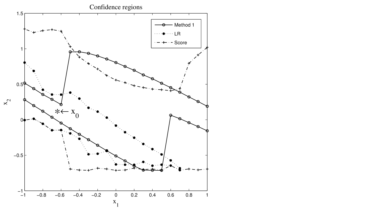
Figure 1: Confidence regions for the $\boldsymbol{\pi}_{0}$th percentile using the three interval estimation methods.

From equation (4.8), the $95\%$ confidence region of $\mathbf{S}_{\boldsymbol{\pi}_{0}}(\boldsymbol{\delta})$ using the LR test (Section 4.2) is given by

$$\{\mathbf{x}=[x_{1},x_{2}]^{\prime}\in R^{2}:L(\mathbf{x})\leq 5.99\},$$ (5.7)

since for $\tau=0.05$, $\chi^{2}_{2,1-\tau}=5.99$. The $95\%$ confidence region of $\mathbf{S}_{\boldsymbol{\pi}_{0}}(\boldsymbol{\delta})$ using the score test (see equation (4.9)) is,

$$\{\mathbf{x}=[x_{1},x_{2}]^{\prime}\in R^{2}:s(\mathbf{x})\leq 5.99\},$$ (5.8)

where $s(\mathbf{x})$ is defined as in Section 4.3.

The confidence regions for the percentiles using the three methods are graphically shown in Figure 1. For plotting the confidence regions we choose $21$ values of $x_{1}$ from the interval $[-1,1]$ at steps of 0.1. For each chosen $x_{1}$, 1000 values of $x_{2}$ are chosen randomly from $[-0.7132,1.2868]$. Let $S_{x_{1}}$ be the set of the selected $x_{2}$ values. To determine the confidence region by method 1, for each value of $x_{1}$ we compute

$$L_{x_{2}}(x_{1}) = min\{x_{2}\in S_{x_{1}}:[x_{1},x_{2}]^{\prime}\text{ is in region (\ref{rbm1})}\}$$

and

$$U_{x_{2}}(x_{1}) = max\{x_{2}\in S_{x_{1}}:[x_{1},x_{2}]^{\prime}\text{ is in region (\ref{rbm1})}\}$$ (5.9)

Then, by plotting $L_{x_{2}}(x_{1})$ and $U_{x_{2}}(x_{1})$ against $x_{1}$ we get the lower and upper bounds of the region, respectively for method 1. We use the same methodology as above to plot the confidence regions by the LR and the score test. From Figure 1, we observe that the confidence regions found by using LR test is narrower than the other two confidence regions, while the score test gives the widest region.

6 Concluding Remarks

In this article, we have introduced a family of link functions which is location and scale invariant and provides local orthogonality between regression and link parameters for multinomial response models. Using a numerical example we are able to show that parametric link function provides a better fit over multivariate logistic link function. We also discussed three different methods for constructing $100(1-\tau)\%$ confidence regions for the $\boldsymbol{\pi}$th percentile.

The percentile estimation methods for multinomial models discussed in this article can be used in clinical trials which are involved in determining dose levels having desired probabilities of both toxicity and efficacy, namely Phase I/II trials (Gooley et al., 1994; Thall and Russell, 1998; O’Quigley et al., 2001). By applying the above interval estimation methods experimenters will be able to find confidence regions of dose levels with tolerable toxicity and the desired efficacy.

There has been a recent rise of interest among researchers to find designs for logistic regression models which are robust to link misspecification. Biedermann et al. (2006) and Woods et al. (2006) propose robust designs by considering a finite set of plausible link functions while Adewale and Xu (2010) uses the family of link functions of Aranda-Ordaz (1981) in their approach. In the future we plan to use the family of link functions proposed in this article to determine designs for multinomial models which are robust to an incorrectly assumed link function.

References

- Adewale and Xu (2010) Adewale, A. J., Xu, X., 2010. Robust designs for generalized linear models with possible overdispersion and misspecified link functions. Computational Statistics and Data Analysis 54, 875–890.
- Agresti (2002) Agresti, A., 2002. Categorical Data Analysis, 2nd Edition. Wiley, New York.
- Aranda-Ordaz (1981) Aranda-Ordaz, F. J., 1981. On two families of transformations to additivity for binary response data. Biometrika 61, 357–363.
- Biedermann et al. (2006) Biedermann, S., Dette, H., Pepelyshev, A., 2006. Some robust design strategies for percentile estimation in binary response models. The Canadian Journal of Statistics 4, 603–622.
- Carter et al. (1986) Carter, W. H., Jr., Chinchilli, V. M., Wilson, J. D., Campbell, E. D., Kessler, F. K., Carchman, R. A., 1986. An asymptotic confidence region for the from the logistic response surface for a combination of agents. The American Statistician 40, 124–128.
- Cox and Reid (1987) Cox, D. R., Reid, N., 1987. Parameter orthogonality and approximate conditional inference. Journal of the Royal Statistical Society 49, 1–39.
- Czado (1989) Czado, C., 1989. Link misspecification and data selected transformations in binary regression models. Tech. rep., Ph.D. Thesis. School of Operations Research and Industrial Engineering, Cornell University, Ithaca, NY.
- Czado (1992) Czado, C., 1992. On link selection in generalized linear models. In: Fahrmeir, L., Francis, B., Gilchrist, R., Tutz, G. (Eds.), Lecture Notes in Statistics. Vol. 78. Springer, New York, pp. 60–65.
- Czado (1993) Czado, C., 1993. Fitting generalized linear models with parametric link in S. Tech. Rep. 93-26, Department of Mathematics and Statistics, York University, North York, Canada.
- Czado (1997) Czado, C., 1997. On selecting parametric link transformation families in generalized linear models. Journal of Statistical Planning and inference 61, 125–139.
- Czado and Santner (1992) Czado, C., Santner, T. J., 1992. The effect of link misspecilication on binary regression analysis. Journal of Statistical Planning and Inference 33, 213–231.
- Fahrmeir and Tutz (2001) Fahrmeir, L., Tutz, G., 2001. Multivariate Statistical Modelling Based on Generalized Linear Models, 2nd Edition. Springer, New York.
- Gennings et al. (1994) Gennings, C., Carter, W. H., Jr., Martin, B. R., 1994. Drug interactions between morphine and marijuana. In: Lange, N., Ryan, L., Billard, L., Brillinger, D., Conquest, L., Greenhouse, J. (Eds.), Case Studies in Biometry. Wiley, New York, pp. 429–451.
- Genter and Farewell (1985) Genter, F. C., Farewell, V., 1985. Goodness-of-link testing in ordinal regression models. The Canadian Journal of Statistics 13, 37–44.
- Gooley et al. (1994) Gooley, T., Martin, P., Fisher, L., Pettinger, M., 1994. Simulation as a design tool for phase I/II clinical trials: An example from bone marrow transplantation. Controlled Clinical trials 15, 450–462.
- Guerrero and Johnson (1982) Guerrero, V., Johnson, R., 1982. Use of the box cox transformation with binary response models. Biometrika 69, 309–314.
- Hamilton (1979) Hamilton, M. A., 1979. Robust estimates of the . Journal of the American Statistical Association 74, 344–354.
- Huang (2001) Huang, Y., 2001. Interval estimation of the when a logistic dose-response curve is incorrectly assumed. Computational Statistics and Data Analysis 36, 525–537.
- Huyer and Neumaier (1999) Huyer, W., Neumaier, A., 1999. Global optimization by multilevel coordinate search. Journal of Global Optimization 14, 331–355.
- Lang (1999) Lang, J. B., 1999. Bayesian ordinal and binary regression models with a parametric family of mixture links. Computational Statistics and Data Analysis 31, 59–87.
- Li and Duan (1989) Li, K., Duan, N., 1989. Regression analysis under link violation. The Annals of Statistics 17, 1009–1052.
- Li and Wiens (2011) Li, P., Wiens, D. P., 2011. Robustness of design in dose-response studies. Journal of the Royal Statistical Society 73, 215–238.
- Mukhopadhyay and Khuri (2008) Mukhopadhyay, S., Khuri, A. I., 2008. Optimization in a multivariate generalized linear model situation. Computational Statistics and Data Analysis 52, 4625 –4634.
- O’Quigley et al. (2001) O’Quigley, J., Hughes, M., Fenton, T., 2001. Dose-finding designs for HIV studies. Biometrics 57, 1018–1029.
- Pregibon (1980) Pregibon, D., 1980. Goodness of link tests for generalized linear models. Journal of the Royal Statistical Society 29, 15–24.
- Prentice (1975) Prentice, R. L., 1975. Discrimination among some parametric models. Biometrika 64, 607–614.
- Prentice (1976) Prentice, R. L., 1976. A generalization of the probit and logit methods for dose response curves. Biometrics 32, 761–768.
- Rao (1973) Rao, C. R., 1973. Linear Statistical Inference and its Application, 2nd Edition. Wiley, New York.
- Stukel (1988) Stukel, T. A., 1988. Generalized logistic models. Journal of the American Statistical Association 83, 426–431.
- Thall and Russell (1998) Thall, P., Russell, K., 1998. A strategy for dose-finding and safety monitoring based on eficacy and adverse outcomes in phase I/II clinical trials. Biometrics 54, 251–264.
- Williams (1986) Williams, D. A., 1986. Interval estimation of the median lethal dose. Biometrics 42, 641–645.
- Woods et al. (2006) Woods, D. C., Lewis, S. M., Eccleston, J. A., Russell, K. G., 2006. Designs for generalized linear models with several variables and model uncertainty. Technometrics 48, 284–292.