An Approach to Making SPAI and PSAI Preconditioning Effective for Large Irregular Sparse Linear Systems

Abstract

We investigate the SPAI and PSAI preconditioning procedures and shed light on two important features of them: (i) For the large linear system $Ax=b$ with $A$ irregular sparse, i.e., with $A$ having $s$ relatively dense columns, SPAI may be very costly to implement, and the resulting sparse approximate inverses may be ineffective for preconditioning. PSAI can be effective for preconditioning but may require excessive storage and be unacceptably time consuming; (ii) the situation is improved drastically when $A$ is regular sparse, that is, all of its columns are sparse. In this case, both SPAI and PSAI are efficient. Moreover, SPAI and, especially, PSAI are more likely to construct effective preconditioners. Motivated by these features, we propose an approach to making SPAI and PSAI more practical for $Ax=b$ with $A$ irregular sparse. We first split $A$ into a regular sparse $\tilde{A}$ and a matrix of low rank $s$. Then exploiting the Sherman–Morrison–Woodbury formula, we transform $Ax=b$ into $s+1$ new linear systems with the same coefficient matrix $\tilde{A}$, use SPAI and PSAI to compute sparse approximate inverses of $\tilde{A}$ efficiently and apply Krylov iterative methods to solve the preconditioned linear systems. Theoretically, we consider the non-singularity and conditioning of $\tilde{A}$ obtained from some important classes of matrices. We show how to recover an approximate solution of $Ax=b$ from those of the $s+1$ new systems and how to design reliable stopping criteria for the $s+1$ systems to guarantee that the approximate solution of $Ax=b$ satisfies a desired accuracy. Given the fact that irregular sparse linear systems are common in applications, this approach widely extends the practicability of SPAI and PSAI. Numerical results demonstrate the considerable superiority of our approach to the direct application of SPAI and PSAI to $Ax=b$.

1 Introduction

Krylov iterative solvers [15, 30] have been very popular for the large sparse linear system

$$Ax=b,$$ (1)

where $A$ is a real nonsingular $n\times n$ matrix and $b$ is an $n$-dimensional real vector. However, when $A$ has bad spectral property or is ill conditioned, the solvers generally exhibit extremely slow convergence and necessitate preconditioning techniques. Sparse approximate inverse (SAI) preconditioning aims to compute a preconditioner $M\approx A^{-1}$ directly so as to improve the conditioning of (1) for the vast majority of problems, and it is nowadays one class of important general-purpose preconditioning techniques for Krylov solvers [3, 30]. There are two typical kinds of SAI preconditioning approaches. One of them constructs a factorized sparse approximate inverse. An effective algorithm of this kind is the approximate inverse (AINV) algorithm, which is derived from the incomplete (bi)conjugation procedure [4, 5]. The other kind is based on F-norm minimization and is inherently parallelizable. This kind of preconditioners are more robust and general. The approach constructs $M\approx A^{-1}$ by minimizing $\|AM-I\|_{F}$ for a specified pattern of $M$ that is either prescribed in advance or determined adaptively, where $\|\cdot\|_{F}$ denotes the F-norm of a matrix. The most popular F-norm minimization-based SAI preconditioning technique may be the adaptive sparse approximate inverse (SPAI) procedure [17], which has been widely used. The adaptive power sparse approximate inverse (PSAI) procedure with dropping, advanced in [27] and called PSAI($tol$), is also an effective F-norm minimization-based SAI preconditioning technique and has been shown to be at least competitive with SPAI numerically and can outperform SPAI for some practical problems. A hybrid version, i.e., the factorized approximate inverse (FSAI) preconditioning based on F-norm minimization, has been introduced in [28]. FSAI is generalized to block form, called BFSAI in [24]. An adaptive algorithm in [25] is presented that generates automatically the nonzero pattern of a BFSAI preconditioner. In addition, the idea of F-norm minimization is generalized in [20] by introducing a sparse readily inverted target matrix $T$. $M$ is then computed by minimizing $\|AM-T\|_{F,H}$ over a space of matrices with a prescribed sparsity pattern, where $\|\cdot\|_{F,H}$ is the generalized F-norm defined by $\|A\|^{2}_{F,H}=\langle A,A\rangle_{F,H}=trace(A^{T}HA)$ with $H$ being some symmetric positive definite matrix, the superscript $T$ denotes the transpose of a matrix or vector. A good comparison of factorized SAI and F-norm minimization based SAI preconditioning approaches can be found in [6]. Spare approximate inverses have been shown to provide effective smoothers for multigrid; see, e.g., [10, 11, 31, 33]. For a comprehensive survey on preconditioning techniques, we refer the reader to [3, 14].

Throughout this paper, we will frequently use two keywords “regular sparse” and “irregular sparse” for a matrix. By regular sparse, we, qualitatively and sensibly, mean that all the columns of the matrix are sparse, and no column has much more nonzero entries than the others. By irregular sparse, we mean that there are some (relatively) dense columns, each of which has considerably more nonzero entries than the other sparse columns. We call such columns irregular and denote by $s$ the number of them. Problem (1) with $A$ irregular sparse is quite common and arises in semiconductor device problem, power network problem, circuit simulation, optimization problem and many others [12]. Quantitatively, we will declare a matrix irregular sparse if it has at least one column that has $10p$ nonzero entries or more, where $p$ is the average number of nonzero entries per column. Under this definition, we investigate all the matrices in the University of Florida sparse matrix collection [12], which contains 2649 matrices and of them 1978 are square. We find that 682 out of these 1978 matrices are irregular sparse. That is, 34% of the matrices in the collection are irregular sparse. In the collection, there are some social networks, citation networks, and other graphs that are not typically viewed as linear systems. They often have dense columns. But even if these matrices are removed, there are 30% irregular sparse matrices, 464 out of 1554, in the collection. So irregular sparse linear systems have a wide broad of applications.

The possible success of any SAI preconditioning procedure is based on the crucial assumption that $A$ has good sparse approximate inverses. Under this assumption, throughout the paper we consider the case that $A$ is irregular sparse. It is empirically observed that good sparse approximate inverses of $A$ are irregular sparse too. In the context, we are concerned with the adaptive SPAI and PSAI($tol$) procedures. As is seen, since the number of nonzero entries in an individual column of the final $M$ in SPAI is bounded by the maximum number of most profitable indices per loop times the maximum loops, a column of $M$ may have not enough nonzero entries. As a result, $M$ obtained by SPAI may not approximate $A^{-1}$ well and thus may be ineffective for preconditioning. Moreover, it can be justified that the SPAI algorithm may be very costly to implement. For PSAI($tol$), we may also suffer the unaffordable overhead from solving some possibly large LS problems (4), although it is more likely to construct effective preconditioners no matter whether $A$ is regular sparse or not. Remarkably, it turns out that the situation mentioned above is improved substantially if $A$ is regular sparse. With reasonable parameters, SPAI and PSAI($tol$) are efficient. Furthermore, SPAI and, especially, PSAI($tol$) are more likely to construct effective sparse approximate inverses.

It is well known [7] that the computational consumption, stability and effectiveness of factorized SAI preconditioners are generally sensitive to reorderings of $A$. Unfortunately, reorderings do not help for SPAI and PSAI($tol$). The reason is that reorderings do not change the irregularity of sparsity patterns of $A$, $A^{-1}$ and good sparse approximate inverses of $A$. Therefore, with reorderings used, SPAI and PSAI($tol$) may still be very costly to implement, and SPAI may still be ineffective for preconditioning. We refer the reader to [3] for the relevant arguments about SPAI, which are valid for PSAI($tol$) as well.

Because of the above features, we naturally come up with the idea of transforming the irregular sparse problem (1) into some regular sparse one(s), on which SPAI and PSAI($tol$) may work well. It will appear that the Sherman–Morrison–Woodbury formula [16, 32] provides us a powerful tool and can be used a key step towards our goal. We present an approach to splitting $A$ into a regular sparse matrix $\tilde{A}$ and a matrix of low rank $s$ and to transforming (1) into the $s+1$ new linear systems with the same coefficient matrix $\tilde{A}$. By exploiting the Sherman–Morrison–Woodbury formula, we can recover the solution of (1) from the ones of the $s+1$ systems directly. We consider numerous practical issues on how to obtain a desired splitting of $A$, how to define and compute an approximate solution of (1) via those of the new systems, and how accurately we should solve the new systems, etc. A remarkable merit of this approach is that SPAI and PSAI($tol$) are efficient to construct possibly effective preconditioners for the new systems, making Krylov solvers converge fast. The price we pay is to solve $s+1$ linear systems. But a great bonus is that we only need to construct one effective sparse approximate inverse $M$ efficiently for the $s+1$ systems. The price is generally insignificant as it is typical that the construction of an effective $M$ dominates the whole cost of Krylov iterations even in a parallel computing environment [1, 3, 6]. As a matter of fact, due to inherent parallelizations of SPAI and PSAI($tol$), SAI type precondtioners are attractive for solving a sequence of linear systems with the same coefficient matrix, as has been addressed in the literature, e.g., [5]. Therefore, given the fact that irregular sparse linear systems are quite common in applications, our approach widely extends the practicality of SPAI and PSAI($tol$).

The paper is organized as follows. In §2, we review SPAI and PSAI($tol$) procedures and shed light on the above-mentioned features for $A$ irregular sparse and regular sparse, respectively. In §3, we describe our new approach for solving (1) with $A$ irregular sparse. In §4 we consider numerous theoretical and practical issues, establishing some results on the nonsingularity of $\tilde{A}$ obtained from certain important and widely useful classes of matrices $A$ and drawing some claims on the conditioning of $\tilde{A}$. In §5, we report numerical experiments to demonstrate the superiority of our approach to SPAI and PSAI($tol$) applied to (1) directly and the superiority of PSAI($tol$) to SPAI for both irregular and regular sparse linear systems. Finally, we conclude the paper in §6.

2 The SPAI and PSAI($tol$) procedures

In this section, we overview the SPAI and PSAI($tol$) procedures and shed light on the facts that (i) SPAI and PSAI($tol$) may be very costly and (ii) SPAI may not be effective for preconditioning if $A$ is irregular sparse.

During loops each of SPAI and PSAI($tol$) solves a sequence of constrained optimization problems of the form

$$\min_{M\in\mathcal{M}}\|AM-I\|_{F},$$ (2)

where $\mathcal{M}$ is the set of matrices with a given sparsity pattern $\mathcal{S}$. Denote by $\mathcal{M}_{k}$ the set of $n$-dimensional vectors whose sparsity pattern is $\mathcal{S}_{k}=\{i|(i,k)\in\mathcal{S}\}$. Then (2) is decoupled into $n$ independent constrained least squares (LS) problems

$$\min_{m_{k}\in\mathcal{M}_{k}}\|Am_{k}-e_{k}\|,\quad k=1,2,\ldots,n$$ (3)

with $e_{k}$ the $k$-th column of the $n\times n$ identity matrix $I$. Here and hereafter, the norm $\|\cdot\|$ denotes the vector 2-norm or the matrix spectral norm. For each $k$, let $\hat{m}_{k}=m_{k}(\mathcal{S}_{k})$, ${\cal L}_{k}$ be the set of indices of nonzero rows of $A(:,{\cal S}_{k})$, $\hat{A}_{k}=A({\cal L}_{k},{\cal S}_{k})$ and $\hat{e}_{k}=e_{k}({\cal L}_{k})$. Then (3) is reduced to the smaller unconstrained LS problems

$$\min_{\hat{m}_{k}}\|\hat{A}_{k}\hat{m}_{k}-\hat{e}_{k}\|,\quad k=1,2,\ldots,n,$$ (4)

which can be solved by the QR decomposition in parallel. SPAI and PSAI($tol$) determine the sparsity pattern $\mathcal{S}_{k}$ dynamically: starting with a simple initial pattern, say the pattern of $e_{k}$, $\mathcal{S}_{k}$ is augmented or adjusted adaptively until the residual norm $\|Am_{k}-e_{k}\|$ falls below a given tolerance or the maximum number of augmentations is reached. The distinction between SPAI and PSAI($tol$) lies in the way that $\mathcal{S}_{k}$ is augmented or adjusted. As is clear from §2.1 and §2.2, the already existing positions of nonzero entries in $m_{k}$ for SPAI are retained in subsequent loops, and at each loop a few most profitable indices added, which are selected from a certain new set generated at the current loop. PSAI($tol$) aims to adaptively drop the entries whose sizes are below certain tolerances and only retain the remaining large ones during the determination of $M$, and $\mathcal{S}_{k}$ is adjusted dynamically by not only absorbing new members but also discarding the positions where the entries of $m_{k}$ become small during loops. In other words, at each loop PSAI($tol$) determines the positions of entries of large magnitude in a globally optimal sense, while SPAI does the job locally by adding a few ones from a local pattern generated at the current loop. Therefore, PSAI($tol$) may capture a more effective sparsity pattern of $A^{-1}$ than SPAI.

2.1 The SPAI procedure

Denote by $\mathcal{S}_{k}^{(l)}$ the sparsity pattern of $m_{k}$ after $l$ loops of augmentation starting with a given initial pattern $\mathcal{S}_{k}^{(0)}$, and by $\mathcal{L}_{k}^{(l)}$ the set of indices of nonzero rows of $A(:,\mathcal{S}_{k}^{(l)})$. Let $\hat{A}_{k}=A(\mathcal{L}_{k}^{(l)},\mathcal{S}_{k}^{(l)}),\hat{e}_{k}=e_{k}(\mathcal{L}_{k}^{(l)})$, and $\hat{m}_{k}$ be the solution of (4). Then the residual of (3) is

$$r_{k}=A(:,\mathcal{S}_{k}^{(l)})\hat{m}_{k}-e_{k}.$$

For $r_{k}\neq 0$, denote by $\mathcal{L}$ the set of indices $l$ for which $r_{k}(l)\neq 0$, and by $\mathcal{N}$ the set of indices of nonzero columns of $A(\mathcal{L},:)$. Then

$$\tilde{\mathcal{J}}=\mathcal{N}\backslash\mathcal{S}_{k}^{(l)}$$ (5)

constitutes the new candidates for augmenting $\mathcal{S}_{k}^{(l)}$ in the next loop. Grote and Huckle [17] suggest to select several most profitable indices from $\tilde{\mathcal{J}}$ and augment them to $\mathcal{S}_{k}^{(l)}$ to obtain a new sparsity pattern $\mathcal{S}_{k}^{(l+1)}$ of $m_{k}$. They do this as follows: for each $j\in\tilde{\mathcal{J}}$, consider the one-dimensional minimization problem

$$\min_{\mu_{j}}\|r_{k}+\mu_{j}Ae_{j}\|,$$ (6)

whose solution is

$$\mu_{j}=-\frac{r_{k}^{T}Ae_{j}}{\|Ae_{j}\|^{2}}.$$ (7)

The 2-norm $\rho_{j}$ of the new residual $r_{k}+\mu_{j}Ae_{j}$ satisfies

$$\rho_{j}^{2}=\|r_{k}\|^{2}-\frac{(r_{k}^{T}Ae_{j})^{2}}{\|Ae_{j}\|^{2}.}$$ (8)

The set $\tilde{\mathcal{S}}_{k}^{(l)}$ of the most profitable indices $j$ consists of those associated with a few, say, 1 to 5, smallest $\rho_{j}$ and is added to $\mathcal{S}_{k}^{(l)}$ to obtain $\mathcal{S}_{k}^{(l+1)}$. Update $\mathcal{L}_{k}^{(l)}$ to get $\mathcal{L}_{k}^{(l+1)}$ by adding the set $\tilde{\mathcal{L}}_{k}^{(l)}$ of indices of new nonzero rows corresponding to $\tilde{S}_{k}^{(l)}$. The new augmented LS problem (4) is solved by updating $\hat{m}_{k}$ instead of resolving it. Proceed in such a way until $\|Am_{k}-e_{k}\|\leq\delta$ or $l$ attains the prescribed maximum $l_{\max}$ of loops, where $\delta$ is a given mildly small tolerance, say $0.1\sim 0.4$.

Remark 1. Let us consider the computational complexity of SPAI. For $A$ regular sparse, it is straightforward to verify that $r_{k}=Am_{k}-e_{k}$ is also sparse, and both $\mathcal{L}$ and $\tilde{\mathcal{J}}$ have only a few elements. As a result, the cardinal number of $\mathcal{S}_{k}^{(l)}$ is small, so is the order of $\hat{A}_{k}$ in (4). Therefore, it is cheap to determine the set $\tilde{\mathcal{S}}_{k}^{(l)}$ of the most profitable indices and solve (4). However, the situation deteriorates severely when $A$ is irregular sparse. For example, assume that the $k$-th column $a_{k}$ of $A$ is relatively dense, and denote $A=(a_{ij})$. If $a_{kk}\neq 0$ and we take $\mathcal{S}_{k}^{(0)}=\{k\}$, the residual $r_{k}=m_{k}(k)a_{k}-e_{k}$ is as dense as $a_{k}$ in the first loop of SPAI, causing that $\mathcal{L}$, ${\mathcal{N}}$ and $\tilde{\mathcal{J}}$ have big cardinal numbers. Keep in mind that $\mathcal{S}_{k}^{(l)}$ has a very small cardinal number for all $l$ as both the maximum of loops and the number of most profitable indices are small. Then it is easily checked that ${\mathcal{L}}$, ${\mathcal{N}}$ and $\tilde{\mathcal{J}}$ always have very big cardinal numbers in subsequent loops. As a consequence, suppose that $a_{k}$ is fully dense, at each loop we have to compute almost $n$ numbers $\rho_{j}$, order them and select the most profitable indices in $\tilde{\mathcal{J}}$. Generally, at some loop, once a nonzero index of $m_{k}$ corresponds to an irregular column of $A$, then the resulting residual $r_{k}$ must be dense, generating big cardinalities of ${\mathcal{L}},\ {\mathcal{N}}$ and $\tilde{\mathcal{J}}$ at the current loop and in subsequent loops. So SPAI may be very costly to implement for $A$ irregular sparse.

Remark 2. SPAI provides a right preconditioner. One should notice that $A^{T}$ may not be so when $A$ is irregular sparse. Naturally, one might apply SPAI to $A^{T}$ and computes a left preconditioner $M$, whose transpose $M^{T}$ is a right preconditioner. However, SPAI may still be very costly to implement in this way, and in fact it may be more costly: Suppose that the $k$-th row $a_{k}^{T}$ of $A^{T}$ is fully dense. Then when computing the $j$-th column $m_{j}$ of $M$, $j=1,2,\ldots,n$, since $a_{k}^{T}$ is dense, we generally have $a_{k}^{T}m_{j}\not=0$. This means that the $k$-th component of the residual $r_{j}=A^{T}m_{j}-e_{j}$ is nonzero and thus $k\in{\mathcal{L}}$ at each loop. As a result, when computing each column $m_{j}$ of $M$, the cardinalities of $\mathcal{N}$ and $\tilde{\mathcal{J}}$ are about $n$ at each loop, and we have to compute almost $n$ numbers $\rho$, order them and select a few most profitable indices at each loop. Such kind of feature is the same for all $j=1,2,\ldots,n$. Consequently, the situation is now more severe than SPAI working on $A$ directly, and generally it is more costly to apply SPAI to $A^{T}$ when $A$ is irregular sparse.

Remark 3. For the irregular sparse $A$, suppose that it has good sparse approximate inverses. Then they are typically irregular sparse too. Suppose the $k$-th column of a good sparse approximate inverse is irregular. The description of SPAI shows that if $a_{k}$ is irregular, i.e., relatively dense, then the sets $\tilde{\mathcal{J}}$ in (5) have big cardinal numbers during loops. Nevertheless, SPAI simply takes the set $\tilde{\mathcal{S}}_{k}^{(l)}$ to be only a few most profitable indices from $\tilde{\mathcal{J}}$ at each loop. If the cardinality of $\tilde{\mathcal{S}}_{k}^{(l)}$ is fixed small, say 5, the default value as suggested and used in [1, 2, 17], then the $k$-th column of $M$ is sparse and may not approximate the $k$-th column of $A^{-1}$ well unless the loops $l_{\max}$ is large enough. Since the number of nonzero entries in an individual column of the final $M$ in SPAI is bounded by the maximum number of most profitable indices per loop times the maximum loops $l_{\max}$, which is fairly small, say 20 (the default value is 5 in [1, 2]), a column of $M$ may have not enough nonzero entries. As a result, $M$ obtained by SPAI may not approximate $A^{-1}$ well and is thus ineffective for preconditioning.

Remark 4. We point out that there are pathological regular sparse matrices whose good sparse approximate inverses are irregular sparse. Thus it is possible, and in fact quite common in practice, that a regular sparse matrix causes problems for SPAI. This is a case for sparse matrices arising from finite differences, volumes or elements of some PDEs. A two-level sparse approximate inverse preconditioning proposed by Chen [9] attempts to handle this class of problems, in which SPAI is used to first compute a right preconditioner $M_{1}$ of $A$ and then compute a left preconditioner $M_{2}$ of the sparsification of $AM_{1}$. Numerically, this procedure can be effective for preconditioning a number of problems, but it lacks theoretical justification and may encounter difficulty since the sparsification of $AM_{1}$ is crucial but it can only be done empirically.

2.2 The PSAI($tol$) procedure

We first review the basic PSAI (BPSAI) procedure [27]. From the Cayley–Hamilton theorem, $A^{-1}$ can be expressed as a matrix polynomial of $A$ of degree $d-1$ with $d\leq n$:

$$A^{-1}=\sum_{i=0}^{d-1}c_{i}A^{i}，$$ (9)

with $A^{0}=I$ and $c_{i}$ $(i=0,1,\ldots,d-1)$ being certain constants. Denote $\mathcal{P}(\cdot)$ by the sparsity pattern of a matrix or vector, and write the matrix $|A|=(|a_{ij}|)$. It is obvious that $\mathcal{P}(A^{-1})\subseteq\mathcal{P}((I+|A|)^{d-1})$. For a given small positive integer $l_{\max}<d$, the pattern $\mathcal{S}$ of a sparse approximate inverse $M$ is taken as a subset of $\mathcal{P}((I+|A|)^{l_{\max}})$ in BPSAI. Therefore, the pattern $\mathcal{S}_{k}$ of the $k$-th column $m_{k}$ of $M$ is a subset of $\bigcup\limits_{l=0}^{l_{\max}}\mathcal{P}(|A|^{l}e_{k})$ since

$$\mathcal{P}((I+|A|)^{l_{\max}})=\bigcup_{l=0}^{l_{\max}}\mathcal{P}(|A|^{l}).$$

The adjustment of $\mathcal{S}_{k}$ for $1\leq k\leq n$ proceeds dynamically as follows. For $l=0,1,\ldots,l_{\max}$, denote by $\mathcal{S}_{k}^{(l)}$ the sparsity pattern of $m_{k}$ at the current loop $l$ and by $\mathcal{L}_{k}^{(l)}$ the set of indices of nonzero rows of $A(:,\mathcal{S}_{k}^{(l)})$. Set $a_{k}^{(l)}=A^{l}e_{k}$. Then $a_{k}^{(l+1)}=Aa_{k}^{(l)}$ with $a_{k}^{(0)}=e_{k}$. The sparsity pattern $\mathcal{S}_{k}^{(l+1)}$ is updated as $\mathcal{S}_{k}^{(l+1)}=\mathcal{P}(a_{k}^{(l+1)})\cup\mathcal{S}_{k}^{(l)}$. In the next loop we solve the augmented LS problem

$$\min\|A(\mathcal{L}_{k}^{(l+1)},\mathcal{S}_{k}^{(l+1)})m_{k}(\mathcal{S}_{k}^{(l+1)})-e_{k}(\mathcal{L}_{k}^{(l+1)})\|$$

with $\mathcal{L}_{k}^{(l+1)}=\mathcal{L}_{k}^{(l)}\cup\tilde{\mathcal{L}}_{k}^{(l)}$, where $\tilde{\mathcal{L}}_{k}^{(l)}$ is the set of indices of new nonzero rows corresponding to the set $\mathcal{P}(a_{k}^{(l+1)})\backslash\mathcal{S}_{k}^{(l)}$. This problem corresponds to the small LS problem (4), whose solution can be updated from $m_{k}(\mathcal{S}_{k}^{(l)})$ efficiently. Proceed in such a way until $\|Am_{k}-e_{k}\|\leq\delta$ or $l>l_{\max}$.

It has been proved in [27, Theorem 1] that for $\mathcal{S}_{k}^{(0)}=\{k\}$, as $l_{\max}$ increases, $M$ obtained by BPSAI may become increasingly denser quickly once one column in $A$ is irregular sparse. In order to control the sparsity of $M$ and construct an effective preconditioner, some reasonable dropping strategies should be used. Two practical PSAI($l\!f\!ill$) and PSAI($tol$) algorithms have been proposed in [27]. PSAI($l\!f\!ill$) aims to retain at most $l\!f\!ill$ entries of large magnitude in $m_{k}$. To be more flexible, $l\!f\!ill$ may vary with $k$. Since an effective sparsity pattern of $A^{-1}$ is generally unknown in advance, it is difficult to prescribe a reasonable $l\!f\!ill$. This is a shortcoming similar to SPAI. In contrast, for the newly computed $m_{k}$ at loop $l$, PSAI($tol$) drops those entries of small magnitude below certain tolerances $tol$ and retains only the ones of large magnitude. Therefore, PSAI($tol$) is more reasonable and reliable to capture an effective sparsity pattern of $A^{-1}$ and determines the corresponding entries. A central issue is the selection of dropping tolerance $tol$. This issue is mathematically nontrivial, and $tol$ has strong effects on the effectiveness of PSAI($tol$) and many other SAI preconditioning procedures. The authors [26] have proposed effective and robust dropping criteria for PSAI($tol$) and all the static F-norm minimization-based SAI preconditioning procedures. For PSAI($tol$), it is shown that, at loop $l\leq l_{\max}$, a nonzero entry $m_{jk}$ is dropped for $1\leq j\leq n$ if

$$|m_{jk}|\leq tol_{k}=\frac{\delta}{nnz(m_{k})\|A\|_{1}},\ k=1,2,\ldots,n,$$ (10)

where $nnz(\cdot)$ is the number of nonzero entries in a vector or matrix, and $\delta<0.5$ is the stopping tolerance for SPAI and BPSAI. We comment that $m_{k}$ in (10) is the newly computed one at loop $l$. This criterion makes $M$ as sparse as possible and meanwhile has similar preconditioning quality to the possibly much denser one obtained by BPSAI [26]. More precisely, for the final $M$ obtained by PSAI($tol$), if (10) is used then the residual norm $\|Am_{k}-e_{k}\|\leq 2\delta,\ k=1,2,\ldots,n$ when the residual norm of each column of the preconditioner obtained by BPSAI falls below $\delta$.

Remark. If $A$ is regular sparse, it is direct to justify that the size of $\hat{A}_{k}$ in (4) is small for a small $l_{\max}$ and it is cheap to solve (4). However, the situation changes sharply for $A$ irregular sparse. Suppose that the $k$-th column $a_{k}$ of $A$ is relatively dense and and take $\mathcal{S}_{k}^{(0)}=\{k\}$. Then the resulting $m_{k}$ is also relatively dense since $\mathcal{S}_{k}^{(1)}=\mathcal{P}(a_{k})\cup\{k\}=\mathcal{P}(a_{k})$. Therefore, (4) is a relatively large LS problem. Since $\mathcal{S}_{k}^{(l+1)}=\mathcal{P}(a_{k}^{(l+1)})\cup\mathcal{S}_{k}^{(l)}$, (4) is always a large LS problem at each subsequent loop $l\leq l_{\max}$. Therefore, if $a_{k}$ is dense, PSAI($tol$) is very costly and impractical.

3 Transformation of (1) into regular sparse linear systems

As we have seen, SPAI and PSAI($tol$) may be very costly to implement for $A$ irregular sparse, and $M$ obtained by SPAI may be ineffective for preconditioning (1). In this section, we attempt to transform (1) into some regular sparse ones, making SPAI and PSAI($tol$) more practical to construct possibly effective $M$. It turns out that the following Sherman–Morrison–Woodbury formula (see [16, p. 50] and [32, p. 330]) provides us a powerful tool for our purpose.

Theorem 1.

Let $U,V\in\mathbb{R}^{n\times s}$ with $s\leq n$. If $A$ is nonsingular, then $A-UV^{T}$ is nonsingular if and only if $I-V^{T}A^{-1}U$ is nonsingular. Furthermore,

$$(A-UV^{T})^{-1}=A^{-1}+A^{-1}U(I-V^{T}A^{-1}U)^{-1}V^{T}A^{-1}.$$ (11)

The formula is typically of interest for $s\ll n$, and it is called the Sherman–Morrison formula when $s=1$. For a good survey on the history and applications, we refer the reader to [18].

For our purpose, assume that the $j_{1},j_{2},\ldots,j_{s}$-th columns of $A$ are irregular and the remaining $n-s$ ones are sparse. Denote by $A_{dc}=(a_{j_{1}},a_{j_{2}},\ldots,a_{j_{s}})$ the matrix consisting of the $s$ irregular columns of $A$, and by $\tilde{A}_{dc}=(\tilde{a}_{j_{1}},\tilde{a}_{j_{2}},\ldots,\tilde{a}_{j_{s}})$ the sparsification of $A_{dc}$ that drops some of its nonzero entries, so that each column of $\tilde{A}_{dc}$ is as sparse as the other $n-s$ columns of $A$. Define $U=A_{dc}-\tilde{A}_{dc}=(u_{1},u_{2},\ldots,u_{2})$. Then the nonzero entries of $U$ are just those dropped ones of $A_{dc}$. Let $\tilde{A}$ be the matrix that is obtained from $A$ by replacing its dense columns $a_{j_{i}}$ by the sparse vectors $\tilde{a}_{j_{i}}$, $i=1,2,\ldots,s$. Then $\tilde{A}$ is regular sparse and satisfies

$$A=\tilde{A}+UV^{T},$$ (12)

where $V=(e_{j_{1}},e_{j_{2}},\ldots,e_{j_{s}})$ with $e_{j_{i}}$ the $j_{i}$-th column of the $n\times n$ identity matrix $I,\ i=1,2,\ldots,s$. Assume that $\tilde{A}$ is nonsingular. Then it follows from (11) that

$$A^{-1}=\tilde{A}^{-1}-\tilde{A}^{-1}U(I+V^{T}\tilde{A}^{-1}U)^{-1}V^{T}\tilde{A}^{-1}.$$ (13)

Therefore, the solution of (1) is

$$x=A^{-1}b=\tilde{A}^{-1}b-(\tilde{A}^{-1}U)(I+V^{T}(\tilde{A}^{-1}U))^{-1}(V^{T}\tilde{A}^{-1}b).$$ (14)

This amounts to solving a new regular sparse linear system

$$\tilde{A}y=b$$ (15)

and the other $s$ regular sparse linear systems

$$\tilde{A}w_{j}=u_{j},\ j=1,2,\ldots,s.$$ (16)

If the exact solutions to (15) and (16) were available, we would get the solution $x$ of (1) from (14) by solving the small $s\times s$ linear system with the coefficient matrix $I+V^{T}(\tilde{A}^{-1}U)$ and the right-hand side $V^{T}\tilde{A}^{-1}b$.

We can summarize the above approach as Procedure *.

Procedure *: Solving the irregular sparse linear system (1)

1:  Find $s$ and $A_{dc}$, and sparsify $A_{dc}$ to get $\tilde{A}_{dc}$. Define $U=A_{dc}-\tilde{A}_{dc}$ and the regular sparse matrix $\tilde{A}=A-UV^{T}$, where $V=(e_{j_{1}},e_{j_{2}},\ldots,e_{j_{s}})$.

2:  Solve $s+1$ linear systems (15) and (16) for $y$ and $w_{1},w_{2},\ldots,w_{s}$, respectively.

3:  Let $W=(w_{1},w_{2},\ldots,w_{s})=\tilde{A}^{-1}U$ and compute the solution $x$ of $Ax=b$ by

$$x=A^{-1}b=y-W(I+V^{T}W)^{-1}(V^{T}y).$$ (17)

For regular sparse systems (15) and (16), we suppose that only iterative solvers are viable in our context. Now, a big and direct reward is that SPAI and PSAI($tol$) can be implemented much more efficiently to construct preconditioners for the $s+1$ regular sparse systems with the same regular sparse coefficient matrix $\tilde{A}$. Furthermore, compared with the irregular sparse case, SPAI is more likely to construct an effective preconditioner now.

4 Theoretical and practical considerations

When iterative solvers are used, recovering an approximate solution of (1) via those of (15) and (16) is quite involved and is not as simple as Procedure * indicates, in which the exact $y$ and $W$ are assumed. In order to use Procedure * to develop a practical iterative solver for (1), we first need to handle several theoretical and practical issues.

The first issue is about the quantitative meaning of irregular columns, by which we define $A_{dc}$. Obviously, like sparsity itself and many other quantities in numerical analysis, it appears impossible to give a precise definition of it. In fact, it is also unnecessary to do so. In our experiments, we empirically find that the threshold $10p$ is a good choice, where $p=\lfloor nnz(A)/n\rfloor$ is the average number of nonzero entries per column of $A$. If the number of nonzero entries in a column exceeds $10p$, then we mark it as an irregular column. Based on this criterion, we determine all the irregular columns of $A$ and the number $s$ of them. Numerically, we have found that other thresholds ranging from $8p$ to $15p$ work well and exhibit no essential difference. So our approach is insensitive to thresholds.

The second issue is which nonzero entries in $A_{dc}$ should be dropped to get $\tilde{A}_{dc}$ and generate $\tilde{A}$. In principle, the number $\hat{p}$ of nonzero entries in each column of $\tilde{A}_{dc}$ should be comparable to $p$. For the choice of $\hat{p}$, to be unique, we simply propose taking $\hat{p}=p$. Given such $\hat{p}$, there may be many dropping ways. Two obvious approaches can be adopted. The first approach is to retain the diagonal and the $p-1$ nonzero entries nearest to the diagonal in each column of $A_{dc}$. The second approach is to retain the diagonal and the other $p-1$ largest entries in magnitude of each column of $A_{dc}$. Numerically, two approaches have exhibited very similar behavior. Therefore, we will take the first approach and report the results obtained.

The third issue is on the non-singularity of $\tilde{A}$, which is crucial both in theory and practice. First of all, we present the following results.

Theorem 2.

$\tilde{A}$ constructed above is nonsingular for the following classes of matrices:

1. $A$ is strictly (row or column) diagonally dominant.

2. $A$ is irreducibly (row or column) diagonally dominant.

3. $A$ is an $M$-matrix.

Proof.

(i). If $A$ is strictly (row or column) diagonally dominant, $\tilde{A}$ is so too since it removes some off-diagonal nonzero entries of $A$. Therefore, $\tilde{A}$ is nonsingular [34, p. 23].

(ii). For $A$ irreducibly (row or column) diagonally dominant, $\tilde{A}$ is either irreducible or reducible. If $\tilde{A}$ is irreducible, then it must be irreducibly (row or column) diagonally dominant. So $\tilde{A}$ is nonsingular [34, p. 23].

If $\tilde{A}$ is reducible, without loss of generality we suppose that there is a permutation matrix $P$ such that

$$P\tilde{A}P^{T}=\left(\begin{array}[]{cc}\tilde{A}_{11}&\tilde{A}_{12}\\ 0&\tilde{A}_{22}\end{array}\right),$$

where $\tilde{A}_{11}$ and $\tilde{A}_{22}$ are irreducibly square matrices. Since $A$ is irreducibly (row or column) diagonally dominant, $PAP^{T}$ is so too. Partition

$$PAP^{T}=\left(\begin{array}[]{cc}A_{11}&A_{12}\\ A_{21}&A_{22}\end{array}\right)$$

conformingly. Then each of $A_{12}$ and $A_{21}$ must have nonzero entries; otherwise, $A$ is reducible. So $A_{11}$ and $A_{22}$ must be (row or column) diagonally dominant, and at least one row or column in each of them is strictly diagonally dominant. Note that all the nonzero entries of $P\tilde{A}P^{T}$ are the same as the corresponding ones of $PAP^{T}$. Therefore, $\tilde{A}_{11}$ and $\tilde{A}_{22}$ are (row or column) diagonally dominant, and at least one row or column in each of them is strictly diagonally dominant. So, both $\tilde{A}_{11}$ and $\tilde{A}_{22}$ are (row or column) diagonally dominant. Since $\tilde{A}_{11}$ and $\tilde{A}_{22}$ are irreducible, both of them are nonsingular [34, p. 23], which means that $P\tilde{A}P^{T}$ is nonsingular, so is $\tilde{A}$.

(iii). By the definition in [34, p. 61], an $M$-matrix assumes its non-singularity. Theorem 3.25 of [34, p. 91] states that any matrix $C$ obtained from the nonsingular $M$-matrix $A$ by setting certain off-diagonal entries of $A$ to zero is also a nonsingular $M$-matrix. Since our $\tilde{A}$ is just such a $C$, it is nonsingular. ∎

Three classes of matrices in the theorem have a wide broad of applications, e.g., discretizations of second-order ODEs and elliptic PDEs, quantum chemistry, information theory, stochastic process, systems theory, networks and modern economics, to name only a few. Strictly row diagonally dominant matrices are a class of special $H$-matrices; see [34, Theorem 3.27, p. 92]. Actually, the first two classes of matrices in the theorem can be extended to more general forms, as the following corollary states.

Corollary 3.

$\tilde{A}$ is nonsingular for the following matrices:

1. There exists a nonsingular diagonal matrix $D$ for which $AD$ or $DA$ is strictly row or column diagonally dominant, respectively.

2. There exist permutation matrices $P$ and $Q$ for which $PAQ$ is strictly (row or column) diagonally dominant.

3. There are a nonsingular diagonal matrix $D$ and permutation matrices $P$ and $Q$ for which $(PAQ)D$ or $D(PAQ)$ is strictly row or column diagonally dominant.

4. The irreducible analogues of the matrices in (i)–(iii).

5. $A$ is a H-matrix.

Proof.

The proofs of Parts (i)–(iv) are direct from those of Theorem 2. Assertion 5 holds because of a result of [21, p. 124], which states that a necessary and sufficient condition for $A$ to be a $H$-matrix is that there exists a nonsingular diagonal matrix $D$ for which $AD$ is strictly row diagonally dominant. ∎

From the proof of (v) in Corollary 3, we see that H-matrices are a subclass of matrices in (i).

There should be more classes of matrices for which the resulting $\tilde{A}$ is nonsingular theoretically. We do not pursue this topic further in this paper. For a general real-world nonsingular $A$ even though it does not belong to the classes of matrices in Theorem 2 and Corollary 3.

The fourth issue is on the conditioning of $\tilde{A}$. For a general $A$, it is possible to get either a well-conditioned or ill-conditioned $\tilde{A}$. Given that $A$ is generally ill conditioned, the former is more preferable, but we should not expect too much and the latter is more possible. Theoretically speaking, $\tilde{A}$ may be worse or better conditioned than $A$. For a general irregular sparse $A$, numerical experiments will indicate that $\tilde{A}$ is rarely worse conditioned and in fact often, though not always, better conditioned than $A$.

However, for the first and third classes of matrices in Theorem 2, we can analyze the conditioning of $\tilde{A}$ and show that $\tilde{A}$ may be generally better conditioned than $A$. More precisely, for a strictly (row or column) diagonally dominant matrix $A$, it is expected that the 1-norm condition number $\kappa_{1}(\tilde{A})$ or the infinity norm condition number $\kappa_{\infty}(\tilde{A})$ is generally no more and may be considerably smaller than $\kappa_{1}(A)$ or $\kappa_{\infty}(A)$. Similar claims hold for an $M$-matrix $A$. Next we first look into the case that $A$ is strictly row diagonally dominant. The case that $A$ is strictly column diagonally dominant can be treated similarly. Denote $\tilde{A}=(\tilde{a}_{ij})$, and define the quantities

$$\beta_{i} = |a_{ii}|-\sum_{j\not=i}|a_{ij}|,\ i=1,2,\ldots,n,$$

$$\tilde{\beta}_{i} = |\tilde{a}_{ii}|-\sum_{j\not=i}|\tilde{a}_{ij}|,\ i=1,2,\ldots,n.$$

Since that $\tilde{a}_{ii}=a_{ii}$ and all the nonzero entries $\tilde{a}_{ij}=a_{ij}$, we have $\tilde{\beta}_{i}\geq\beta_{i},\ i=1,2,\ldots,n$, with some strict inequalities holding as $\tilde{A}$ drops some off-diagonal nonzero entries in the $s$ irregular columns of $A$. More precisely, from the definitions of $\tilde{\beta}_{i}$ and $\beta_{i}$, it can be easily verified that if $i$ is in the set of the row indices of nonzero entries in $U$ then $\tilde{\beta}>\beta_{i}$. The number of such $i$ is (much) bigger than $s$ and can be very near to $n$ whenever $A$ has a fully dense column as $n-p$ nonzero entries are dropped from an irregular column and put into a column of $U$. Since $A$ is strictly row diagonally dominant, we have $\beta_{i}>0,\,i=1,2,\ldots,n$. A result of [19, p. 154] gives the following general bounds

$$\|A^{-1}\|_{\infty} \leq \frac{1}{\min_{i}\beta_{i}},$$

$$\|\tilde{A}^{-1}\|_{\infty} \leq \frac{1}{\min_{i}\tilde{\beta}_{i}}$$

with $\|A^{-1}\|_{\infty}=1/\beta$ if all $\beta_{i}=\beta$ and $\|{\tilde{A}}^{-1}\|_{\infty}=1/\tilde{\beta}$ if all $\tilde{\beta}_{i}=\tilde{\beta}$; see, e.g., [35]. Since $\tilde{\beta}_{i}\geq\beta_{i}$ with some strict inequalities holding, the bound for $\|\tilde{A}^{-1}\|_{\infty}$ can be smaller than that for $\|A^{-1}\|_{\infty}$. On the other hand, it always holds that

$$\|\tilde{A}\|_{\infty}\leq\|A\|_{\infty}.$$

So, $\kappa_{\infty}(\tilde{A})=\|\tilde{A}\|_{\infty}\|\tilde{A}^{-1}\|_{\infty}$ is generally no more than $\kappa_{\infty}(A)=\|A\|_{\infty}\|A^{-1}\|_{\infty}$ and may be considerably smaller than the latter, provided that some dropped nonzero entries $a_{ij}$ from $A$ are not small. For $A$ strictly column diagonally dominant, we define similar $\tilde{\beta}_{i}$ and $\beta_{i}$ in the column sense. Then similar discussions and the same claims can be made for the 1-norm condition number $\kappa_{1}(\tilde{A})$ and $\kappa_{1}(A)$. The unique difference is that the number of the corresponding $\tilde{\beta}_{i}>\beta_{i}$ in the column sense is exactly $s$ since $A$ and $\tilde{A}$ only have $s$ different columns. Therefore, for $A$ strictly (row or column) diagonally dominant, it is expected that $\tilde{A}$ is better conditioned than $A$.

For $A$ an $M$-matrix, define

$$r_{i}(A)=\sum_{j=1}^{n}a_{ij},i=1,2,\ldots,n.$$

It is known that $a_{ii}>0$ and $a_{ij}\leq 0$ for $j\not=i$ by the definition of $M$-matrix. Then it is seen from $\beta_{i}$ defined above that $r_{i}(A)=\beta_{i},\ i=1,2,\ldots,n$. Similarly, we have $r_{i}(\tilde{A})=\tilde{\beta}_{i},\ i=1,2,\ldots,n$. It is proved in [22] that if there is a positive diagonal matrix $D$ such that

$$r_{i}(AD)>0,\ i=1,2,\ldots,n$$

then

$$\frac{1}{\max r_{i}(AD)}\|D\|_{\infty}\leq\|A^{-1}\|_{\infty}\leq\frac{1}{\min r_{i}(AD)}\|D\|_{\infty}$$

and furthermore

$$\|A^{-1}\|_{\infty}=\frac{1}{r(AD)}\|D\|_{\infty}$$

if $r_{i}(AD)=r(AD),\ i=1,2,\ldots,n$. Note that we have $r_{i}({\tilde{A}}D)\geq r_{i}(AD)$ with some strict inequalities holding as $\tilde{A}$ drops some negative off-diagonal entries $a_{ij}$ from $A$ and $D$ is positive. Thus, the upper bound for $\|{\tilde{A}}^{-1}\|_{\infty}$ is generally smaller than that for $\|A^{-1}\|_{\infty}$. Noticing that $\|\tilde{A}\|_{\infty}\leq\|A\|_{\infty}$, we expect that $\kappa_{\infty}(\tilde{A})$ is generally no more and can be smaller than $\kappa_{\infty}(A)$. Similar discussions and claim go to $DA$ and the 1-norm condition numbers of $A$ and $\tilde{A}$.

The fifth issue is on the existence of good sparse approximate inverses of $\tilde{A}$. The existence is generally definitive. We argue as follows: Since ${\mathcal{P}}(\tilde{A})\subset{\mathcal{P}}(A)$, for a given positive integer $l_{\max}$, we have ${\mathcal{P}}((|\tilde{A}|^{T}|\tilde{A}|)^{l_{\max}}\tilde{A}^{T})\subset{\mathcal{P}}((|A|^{T}|A|)^{l_{\max}}A^{T})$ and ${\mathcal{P}}((I+|\tilde{A}|)^{l_{\max}})\subset{\mathcal{P}}((I+|A|)^{l_{\max}})$. Assume that we take the initial sparsity ${\mathcal{S}}^{(0)}={\mathcal{P}}(I)$ and implement SPAI and PSAI($tol$) $l_{\max}$ loops for $A$. Then it is known [23, 27] that the sparsity patterns of $M$ obtained by SPAI and PSAI($tol$) are bounded by ${\mathcal{P}}((|A|^{T}|A|)^{l_{\max}}A^{T})$ and ${\mathcal{P}}((I+|A|)^{l_{\max}})$, respectively. The same are true for the sparsity patterns of $M$ obtained by SPAI and PSAI($tol$) for $\tilde{A}$. This means that the effective envelops for the sparsity patterns of $M$ obtained by SPAI and PSAI($tol$) for $\tilde{A}$ are contained in those for $A$ for the same $l_{\max}$. As a consequence, it is expected that $\tilde{A}$ has good sparse approximate inverses when $A$ does.

The last important issue is how to select stopping criteria for Krylov iterations for $s+1$ linear systems so as to recover an approximate solution of (1) with the prescribed accuracy. It is seen from (17) that the solution $x$ of (1) is formed from the ones of the $s+1$ new systems. Recall that the $s+1$ linear systems are now supposed to be solved approximately by preconditioned Krylov solvers. Our concerns are (i) how to define an approximate solution $\hat{x}$ from the $s+1$ approximate solutions of (15) and (16), and (ii) how accurately we should solve (15) and (16) such that $\hat{x}$ satisfies $\frac{\|r\|}{\|b\|}=\frac{\|b-A\hat{x}\|}{\|b\|}<\varepsilon$. As it appears below, it is direct to settle down the first concern, but the second concern is involved.

Theorem 4.

Let $\hat{y}$ and $\hat{w}_{j},\ j=1,\ldots,s$, be the approximate solutions of (15) and (16), respectively, and define $\hat{W}=(\hat{w}_{1},\ldots,\hat{w}_{s})$ and the residuals $r_{\hat{y}}=b-\tilde{A}\hat{y}$, $r_{\hat{w}_{j}}=u_{j}-\tilde{A}\hat{w}_{j}$. Assume that $I+V^{T}\hat{W}$ is nonsingular with $V=(e_{j_{1}},e_{j_{2}},\ldots,e_{j_{s}})$, and define $c=\|(I+V^{T}\hat{W})^{-1}(V^{T}\hat{y})\|$. Take

$$\hat{x}=\hat{y}-\hat{W}(I+V^{T}\hat{W})^{-1}(V^{T}\hat{y})$$ (18)

to be an approximate solution of (1). Then if

$$\frac{\|r_{\hat{y}}\|}{\|b\|}<\frac{\varepsilon}{2}$$ (19)

and

$$\frac{\|r_{\hat{w}_{j}}\|}{\|u_{j}\|}<\frac{\|b\|}{2\sqrt{s}c\|u_{j}\|}\varepsilon,\ j=1,2,\ldots,s,$$ (20)

we have

$$\frac{\|r\|}{\|b\|}=\frac{\|b-A\hat{x}\|}{\|b\|}<\varepsilon.$$ (21)

Proof.

Replacing $W$ and $y$ by their approximations $\hat{W}$ and $\hat{y}$ in (17), we get (18), which is naturally an approximate solution of (1). Define $R_{\hat{W}}=U-\tilde{A}\hat{W}$. We obtain

$$r =b-A\hat{x}=b-A\hat{y}+A\hat{W}(I+V^{T}\hat{W})^{-1}(V^{T}\hat{y})$$

$$=b-(\tilde{A}+UV^{T})\hat{y}+(\tilde{A}+UV^{T})\hat{W}(I+V^{T}\hat{W})^{-1}(V^{T}\hat{y})$$

$$=r_{\hat{y}}-UV^{T}\hat{y}+UV^{T}\hat{W}(I+V^{T}\hat{W})^{-1}(V^{T}\hat{y})+\tilde{A}\hat{W}(I+V^{T}\hat{W})^{-1}(V^{T}\hat{y})$$

$$=r_{\hat{y}}-U(I-V^{T}\hat{W}(I+V^{T}\hat{W})^{-1})(V^{T}\hat{y})+\tilde{A}\hat{W}(I+V^{T}\hat{W})^{-1}(V^{T}\hat{y})$$

$$=r_{\hat{y}}-U(I-(I+V^{T}\hat{W}-I)(I+V^{T}\hat{W})^{-1})(V^{T}\hat{y})+\tilde{A}\hat{W}(I+V^{T}\hat{W})^{-1}(V^{T}\hat{y})$$

$$=r_{\hat{y}}-U(I+V^{T}\hat{W})^{-1}(V^{T}\hat{y})+\tilde{A}\hat{W}(I+V^{T}\hat{W})^{-1}(V^{T}\hat{y})$$

$$=r_{\hat{y}}-R_{\hat{W}}(I+V^{T}\hat{W})^{-1}(V^{T}\hat{y}),$$

from which it follows that

$$\|r\|\leq\|r_{\hat{y}}\|+c\|R_{\hat{W}}\|\leq\|r_{\hat{y}}\|+c\|R_{\hat{W}}\|_{F}.$$ (22)

By definition of $c$ and $R_{\hat{W}}(:,j)=r_{\hat{w}_{j}}$, we have $\|R_{\hat{W}}\|_{F}=\sqrt{\sum_{j=1}^{s}\|r_{\hat{w}_{j}}\|^{2}}$. If (19) and

$$\frac{\|r_{\hat{w}_{j}}\|}{\|b\|}<\frac{\varepsilon}{2\sqrt{s}c},\ j=1,2,\ldots,s,$$

it is seen from (22) that (21) holds. Since the above relation is just (20), the theorem holds. ∎

We point out that because of (22) our stopping criterion (20) may be conservative. Furthermore, $c$ is moderate if $I+V^{T}\hat{W}$ is well conditioned, and it may be large if $I+V^{T}\hat{W}$ is ill conditioned. Since $s$ is supposed very small, this theorem indicates that the $s$ linear systems (16) need to be solved with the accuracy at the level of $\varepsilon$. We may solve them by Krylov solvers either simultaneously in the parallel environment or independently in the sequential environment. An alternative approach is to solve them using block Krylov solvers. Note that $c$ cannot be computed until iterations for (15) and (16) terminate, but the stopping criterion (20) depends on $c$. Therefore, the computation of $c$ and termination of iterations interacts. In implementations, we simply replace $c$ by 1 in (20) and stop iterative solvers for the $s$ systems (16) with the modified accuracy requirement. Because of this inaccuracy, (21) may fail to meet but $\|r\|/\|b\|$ should be at the level of $\varepsilon$. In later numerical experiments, we will find that $c=1$ works very well and makes (21) hold for almost all the test problems, and the right-hand sides of (21) are only a little bit bigger than $\varepsilon$ in the rare cases where (21) does not meet.

We make some further comments on (20). For a real-world problem, if $A$ is poorly scaled, it is well known that a preprocessing is generally done that uses scaling to equilibrate $A$ so that its columns and/or rows are nearly the same in norm. Without loss of generality, suppose that $\|b\|$ is comparable to them in size; otherwise, we replace $b$ by a scaled $\hat{b}=\alpha b$ with $\alpha$ a scaling factor and instead solve the equivalent problem $A(\alpha x)=\hat{b}$, so that $\|\hat{b}\|$ is comparable to the norms of columns of the equilibrated $A$. Then the sizes of $\|b\|/\|u_{j}\|$ are typically around $1$. We suppose that such processing is performed. As a result, $s$ linear systems (16) are solved with the accuracy at the level of $\varepsilon$. Therefore, we need not worry about the issue of small $\|b\|/\|u_{j}\|$ for a given problem.

5 Numerical experiments

In this section, we test our approach and compare it with the approach that preconditions (1) by SPAI and PSAI($tol$) directly. We report the numerical experiments obtained by the Biconjugate Gradient Stablized (BiCGStab) with SPAI and PSAI($tol$) preconditioning on (1) and (15), (16), respectively. Such combinations give rise to four algorithms, and we name them Standard-SPAI, New-SPAI, and Standard-PSAI($tol$) and New-PSAI($tol$), abbreviated as S-SPAI, N-SPAI and S-PSAI($tol$), N-PSAI($tol$), respectively.

The experiments consists of three subsections, and our aims are quadruple: (i) We demonstrate the considerable efficiency superiority of N-SPAI to S-SPAI and that of N-PSAI($tol$) to S-PSAI($tol$). (ii) With the same parameters used in SPAI, we show that preconditioners obtained by N-SPAI are more effective than the corresponding ones obtained by S-SPAI. (iii) With the same parameters used in PSAI($tol$), we illustrate that the preconditioners by S-PSAI($tol$) and N-PSAI($tol$) are equally effective for preconditioning each problem, provided that they can be computed. (iv) We illustrate that if the numbers of nonzero entries of preconditioners, i.e., the sparsity of preconditioners, are (almost) the same then PSAI($tol$) is more effective than SPAI for preconditioning both irregular and regular sparse linear systems. The results mean that PSAI($tol$) captures a sparsity pattern of $A^{-1}$ and $\tilde{A}^{-1}$ more effectively than SPAI and thus generate better preconditioners. They also imply that even for regular sparse linear systems, SPAI may be ineffective for preconditioning.

We mention that, for other Krylov solvers, such as BiCG, CGS and the restarted GMRES(20), we have done similar numerical experiments and had the same findings as above. So it suffices to only report and evaluate the results obtained by BiCGStab.

Before testing our approach, we look into all the matrices in the University of Florida sparse matrix collection [12] and give illustrative information on where irregular sparse linear systems come from, how common they are in practice, how big $s$ can be and how dense irregular columns. We divide matrices into their problem domains, and sort them by percentage of matrices in that domain that are irregular. Table 1 lists the relevant information, where “per. irreg” denotes the percentage of irregular matrices in each domain, “#reg. prob” and “#irreg. prob” are the numbers of regular and irregular matrices in each domain, respectively. Matrices labeled as “graphs” in the collection are excluded, many of which are irregular, but not all are linear systems.

Table 1: Statistics of regular/irregular problems in the sparse matrix collection [12]

problem domain	per. irreg	#reg. prob	#irreg. prob
frequency-domain circuit simulation problem	100%	0	4
linear programming problem	100%	0	1
semiconductor device problem	63%	13	22
optimization problem	61%	53	82
power network problem	56%	26	33
circuit simulation problem	51%	124	132
computer graphics/vision problem	33%	2	1
economic problem	33%	44	21
counter-example problem	25%	6	2
eigenvalue/model reduction problem	20%	28	7
material problem	11%	25	3
chemical process simulation problem	11%	62	8
statistical/mathematical problem	11%	8	1
theoretical/quantum chemistry problem	11%	54	7
2D/3D problem	10%	118	13
acoustics problem	8%	12	1
structural problem	5%	287	14
combinatorial problem	3%	28	1
computational fluid dynamics problem	3%	167	5
thermal problem	3%	30	1
electromagnetic problem	2%	49	1
least squares problem	0%	2	0
model reduction problem	0%	47	0
other problem	0%	4	0
random 2D/3D problem	0%	2	0
robotics problem	0%	3	0

The statistics in Table 1 illustrates that irregular sparse linear systems are quite common and come from many applications. Figure 1 depicts many more details. In the top left plot, a circle is a matrix in the collection, the $x$ axis is the order of a square matrix, and the $y$ axis is the number $s$ of dense columns. The steep line is $s=n$, which is not achievable, and the flat line is $s=\sqrt{n}$. This figure plots matrices with at least one dense column. In the top right plot, each dot is a square matrix, the $x$ axis is the mean, i.e., the average number $p$, of nonzero entries in each column, which equals $\lfloor nnz(A)/n\rfloor$, and the $y$ axis is the number of nonzero entries in the densest column divided by the mean for that matrix. The line parallel to the $x$ axis is $y=10$. Matrices have at least one dense column if they reside above the line $y=10$. For each $x$, the bigger $y$, the denser the irregular column. The bottom two plots are the same, but with social networks and other graphs excluded.

These figures further demonstrate that there are very dense columns for many matrices, irregular sparse matrices are common, and $s$ can be quite big.

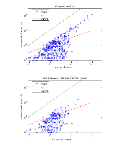
Fig. 1: Illustrations of irregular matrices in the sparse matrix collection [12].

We test our approach on some of the above irregular sparse linear systems. A brief description is presented in Table 2, where $\kappa(A)=\|A\|\|A^{-1}\|$. The right-hand side $b$ of $Ax=b$ was formed by taking the solution $x=(1,1,\ldots,1)^{T}$. Taking the initial approximate solution to be zero for each problem and $\varepsilon=10^{-8}$ in stopping criterion (21), we have found that BiCGStab without preconditioning did not converge for any of the test problems within 500 iterations. We note that cbuckle is symmetric positive definite. So it should be better to design preconditioners to maintain the symmetry of preconditioned matrices, which can be achieved by using factorized or splitting preconditioners, e.g., [4, 24], so that some more efficient symmetric Krylov solvers, e.g., the Conjugate Gradient (CG) or Minimal Residual (MINRES) method, can be applied. In our experiments, however, we used cbuckle in PSAI($tol$) purely for test purposes and treated it as a general matrix.

Table 2: The description of test matrices. “sym” denotes the symmetry of a matrix, and we used the Matlab function condest to estimate the 1-norm condition numbers of the latter seven larger matrices.

Matrix	$n$	$nnz(A)$	$\kappa(A)$	sym	Description
fs_541_3	541	4282	$2.83\times 10^{11}$	No	2D/3D problem
fs_541_4	541	4273	$1.17\times 10^{10}$	No	2D/3D problem
rajat04	1041	8725	$1.64\times 10^{8}$	No	circuit simulation problem
rajat12	1879	12818	$6.91\times 10^{5}$	No	circuit simulation problem
tols4000	4000	8784	$2.36\times 10^{7}$	No	computational fluid dynamics problem
cbuckle	13681	676515	$3.30\times 10^{7}$	Yes	structural problem
ASIC_100k	99340	940621	$1.46\times 10^{11}$	No	circuit simulation problem
dc1	116835	766396	$1.01\times 10^{10}$	No	circuit simulation problem
dc2	116835	766396	$8.86\times 10^{9}$	No	circuit simulation problem
dc3	116835	766396	$1.16\times 10^{10}$	No	circuit simulation problem
trans4	116835	749800	$3.30\times 10^{9}$	No	circuit simulation problem
trans5	116835	749800	$2.32\times 10^{9}$	No	circuit simulation problem

We conducted the numerical experiments on an Intel (R) Core (TM)2 Quad CPU E8400 @ $3.00$GHz with main memory 2 GB under the Linux operating system. The computations were done using Matlab 7.8.0 with the machine precision $\epsilon_{\rm mach}=2.22\times 10^{-16}$, and SPAI preconditioners were constructed by the SPAI 3.2 package [2] of Barnard, Bröker, Grote and Hagemann, which is written in C/MPI. Our PSAI($tol$) code is written in Matlab language for the sequential environment. We used both SPAI and PSAI($tol$) as right preconditioning and took the initial patterns $\mathcal{S}_{k}^{(0)}=\{k\},\ k=1,2,\ldots,n$. We took $c=1$ in (20) and stopped Krylov iterations when (19) and (20) were satisfied with $\varepsilon=10^{-8}$ or 500 iterations were used. The initial approximate solution for each problem was zero vector. With $\hat{x}$ defined by (18), we computed the actual relative residual norm

$$rr=\frac{\|b-A\hat{x}\|}{\|b\|}$$ (23)

and compared it with the required accuracy $\varepsilon=10^{-8}$.

Before performing our algorithms, we carried out row Dulmage–Mendelsohn permutations [13, 29] on the matrices that have zero diagonals, so as to make their diagonals nonzero. This preprocessing, though not necessary theoretically, may be more suitable for taking the initial pattern ${\mathcal{S}}={\mathcal{P}}(I)$ in SPAI, which always retains the diagonals as most profitable indices in $M$. The related Matlab commands are $j=\verb"dmperm"(A)$ and $A=A(j,:)$. We applied dmperm to rajat04, rajat12, tols4000 and ASIC_100k. For all the matrices listed in Table 2, $\tilde{A}$ is constructed by retaining the diagonal entry and $p-1$ nonzero entries nearest to the diagonal and dropping the others in each of the irregular columns of $A$, and $U$ is composed of the dropped nonzero entries. Table 3 shows some useful information on each $A$ and $\tilde{A}$.

Table 3: Some information on $A$ and $\tilde{A}$. $s$: # irregular columns in $A$; $p$: the average number of nonzero entries per column of $A$; $p_{d}$: # nonzero entries in the densest column of $A$. We used Matlab function condest to estimate the 1-norm condition numbers of the last seven larger matrices.

	$n$	$s$	$p$	$p_{d}$	$nnz(A)$	$nnz(\tilde{A})$	$\kappa(A)$	$\kappa(\tilde{A})$
fs_541_3	541	1	7	538	4282	3745	$2.83\times 10^{11}$	$7.86\times 10^{6}$
fs_541_4	541	1	7	535	4273	3739	$1.17\times 10^{10}$	$1.64\times 10^{6}$
rajat04	1041	4	8	642	8725	7306	$1.64\times 10^{8}$	$1.16\times 10^{8}$
rajat12	1879	7	6	1195	12818	9876	$6.91\times 10^{5}$	$6.53\times 10^{5}$
tols4000	4000	18	2	22	8784	8424	$2.36\times 10^{7}$	$2.36\times 10^{7}$
cbuckle	13681	1	49	600	676515	675916	$3.30\times 10^{7}$	$8.06\times 10^{7}$
ASIC$\ast$	99340	122	9	92258	940621	742736	$1.46\times 10^{11}$	$9.28\times 10^{9}$
dc1	116835	55	6	114174	766396	595757	$1.01\times 10^{10}$	$2.17\times 10^{8}$
dc2	116835	55	6	114174	766396	595757	$8.86\times 10^{9}$	$5.81\times 10^{7}$
dc3	116835	55	6	114174	766396	595757	$1.16\times 10^{10}$	$1.52\times 10^{8}$
trans4	116835	55	6	114174	749800	587459	$3.30\times 10^{9}$	$3.46\times 10^{8}$
trans5	116835	55	6	114174	749800	587459	$2.32\times 10^{9}$	$6.54\times 10^{7}$

We have some informative observations from Table 3. As is seen, except cbuckle and tols4000, all the other test matrices have some almost fully dense columns. The matrix cbuckle and tols4000 have 1 and 18 not very dense irregular columns, respectively. Precisely, except cbuckle and tols4000, rajat04 and rajat12 have some irregular columns which have more than $n/2$ nonzero entries, and all the other matrices have some fully dense columns. The table also shows the number $s$ of irregular columns of each $A$ and the percentage $s/n$. The biggest two percentages $0.45\%$ and $0.38\%$ correspond to tols4000 and rajat04, where $s=18$ and $4$, respectively. It is remarkable that the eight $\tilde{A}$ are considerably better conditioned than the corresponding $A$, and their condition numbers are accordingly reduced by roughly one to five orders. For the other three matrices rajat04, rajat12 and cbuckle, each pair of $\tilde{A}$ and $A$ have very near condition numbers.

We next investigate the patterns of entries of large magnitude in the “exact” inverses of an irregular sparse matrix and the regular sparse matrix induced from it. We only take rajat04 as an example. After performing row Dulmage–Mendelsohn permutation on it, we use the Matlab function $\verb"inv"$ to compute $A^{-1}$ and $\tilde{A}^{-1}$ and then drop their nonzero entries whose magnitudes fall below $10^{-3}$. We depict the patterns of sparsified $A^{-1}$ and $\tilde{A}^{-1}$ as (A) and (B) in Figure 2, respectively. It is clear that good approximate inverses of $A$ and $\tilde{A}$ are sparse but there are several dense columns in (A), which means that an effective sparse approximate inverse of $A$ is irregular. On the other hand, the situation is improved substantially in (B), from which it is seen that a good sparse approximate inverse of $\tilde{A}$ is sparser than the matrix in (A). These results typically demonstrate that good sparse approximate inverses of an irregular sparse matrix are also irregular, while the resulting regular sparse matrix $\tilde{A}$ has sparser approximate inverses. We have checked several other test matrices and have had the same findings.

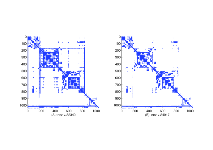
Fig. 2: rajat04: (A) and (B) are the patterns of sparsified $A^{-1}$ and $\tilde{A}^{-1}$, respectively.

In all the later tables, we denote by $T_{setup}$ and $T_{solve}$ the setup (construction) time(sec) of $M$ and the time(sec) of solving the preconditioned linear systems by BiCGStab, respectively, by $spar=nnz(M)/nnz(A)$ or $nnz(M)/nnz(\tilde{A})$ the sparsity of $M$ relative to $A$ or $\tilde{A}$, and by $iter$ the iteration number that BiCGStab used for (1) and the maximum of iteration numbers that BiCGStab used for the $s+1$ systems (15) and (16), respectively. The actual relative residual norm $rr$ defined by (23) is $a\cdot\varepsilon$, and we only list the multiple $a$ in the tables. So $a<1$ indicates that BiCGStab converged with the prescribed accuracy $\varepsilon$. The size of $a$ reflects whether taking $c=1$ in (20) is reliable or not.

5.1 Numerical results obtained by SPAI

We take $\delta=0.4$ as the stopping criterion for SPAI. Since effective sparsity patterns of $A^{-1}$ and $\tilde{A}^{-1}$ are generally unknown in advance, some key parameters, especially the number of most profitable indices per loop involved can only be chosen empirically in order to control the sparsity of $M$ and simultaneously to make $M$ achieve the desired accuracy $\delta$ as much as possible. In the experiments of this subsection, we fix the number of most profitable indices to be 5 per loop, which is also the default value in the SPAI 3.2 code. The maximum $l_{\max}$ of loops is set to 20, bigger than the default value 5 in the code. SPAI terminated whenever $\|Am_{k}-e_{k}\|\leq\delta,\ k=1,2,\ldots,n$ or $l_{\max}$ loops were attained. SPAI is run for $\tilde{A}$ with the same parameters. With the given parameters and the initial pattern ${\cal S}_{k}^{(0)}=\{k\},\ k=1,2,\ldots,n$, the number of nonzero entries per column in the final $M$ is bounded by $1+5\times 19=96$. So if good preconditioners are irregular sparse and there is at least one column whose number of nonzero entries are bigger than 96, then SPAI may be ineffective for preconditioning. We attempt to show that with the same parameters used in SPAI, N-SPAI is much more efficient than S-SPAI, and the former is more effective than the latter for preconditioning. We mention that we have omitted the symmetric positive definite matrix cbuckle since the matrix input in the SPAI 3.2 package is only supported by “real general” Matrix Market coordinate format. Table 4 lists the results.

Table 4: Numerical results obtained by SPAI. $T_{setup}$ and $T_{solve}$: the setup time of $M$ and the time of BiCGStab iterations for the preconditioned linear systems, respectively. The relative residual norm $rr=a\cdot\varepsilon$. $n_{c}$: # columns in $M$ failing to satisfy the accuracy $\delta=0.4$. For S-SPAI, $spar=nnz(M)/nnz(A)$ and $iter$: # iterations of BiCGStab for (1), while for N-SPAI, $spar=nnz(M)/nnz(\tilde{A})$ and $iter$: the maximum of # iterations of BiCGStab for the $s+1$ systems (15) and (16).

	S-SPAI						N-SPAI
	$T_{setup}$	$T_{solve}$	$spar$	$iter$	$a$	$n_{c}$	$T_{setup}$	$T_{solve}$	$spar$	$iter$	$a$	$n_{c}$
fs_541_3	0.33	0.01	1.34	21	0.40	1	0.17	0.01	1.52	8	0.62	0
fs_541_4	0.14	0.01	0.81	14	0.01	1	0.04	0.01	0.91	6	0.68	0
rajat04	1.17	0.01	0.36	31	0.20	6	0.16	0.02	0.40	17	0.57	2
rajat12	3.19	0.01	0.86	48	0.31	3	0.39	0.08	1.08	39	0.80	0
tols4000	0.10	0.02	1.01	3	0.44	6	0.05	0.02	1.02	4	0.48	6
ASIC$\ast$	$*$	$*$	$*$	$*$	$*$	$*$	1619	13.52	0.66	10	1.37	12
dc1	$*$	$*$	$*$	$*$	$*$	$*$	8216	44.07	1.71	351	0.61	1
dc2	$*$	$*$	$*$	$*$	$*$	$*$	6210	41.75	1.62	76	0.75	0
dc3	$*$	$*$	$*$	$*$	$*$	$*$	5243	47.05	1.63	98	0.91	9
trans4	$*$	$*$	$*$	$*$	$*$	$*$	3798	9.13	1.64	39	0.49	0
trans5	$*$	$*$	$*$	$*$	$*$	$*$	3546	20.79	1.57	84	0.65	0

We make some comments on the results. First, we look at the efficiency of constructing $M$ by S-SPAI and N-SPAI. In the table, the notation “$*$” for the last six larger matrices indicates that S-SPAI could not compute $M$ within 100 hours because of the irregular sparsity of $A$. Since each of these six matrices has fully dense irregular columns, the unaffordable time consumption results from the large cardinal numbers of $\tilde{\mathcal{J}}$ and $\mathcal{L}$ in §2.1. More precisely, for a fully dense irregular column of $A$, we have to compute almost the $n$ numbers $\mu_{j}$ in (7), sort almost $n$ indices in $\tilde{\mathcal{L}}$ and select five most profitable indices among them at each loop. Carrying out these tasks is very time consuming. In contrast, N-SPAI did a very good job due to the regular sparsity of $\tilde{A}$. For the other matrices and given the parameters, the two $M$ obtained by S-SPAI and N-SPAI have very similar sparsity, but it is seen from $T_{setup}$ that N-SPAI can be considerably more efficient than S-SPAI, and the former can be several times faster, e.g., six and seven times faster for rajat04 and rajat12, respectively. For the last six larger matrices, N-SPAI computed all the $M$ within no more than half an hour to two hours, drastic improvements over S-SPAI!

Second, we investigate the effectiveness of $M$ for preconditioning. To be more illuminating, we recorded the number $n_{c}$ of columns in $M$ which failed to satisfy the accuracy $\delta=0.4$ for each matrix in S-SPAI or N-SPAI. We have observed that for the first four matrices, the $n_{c}$ produced by N-SPAI are always smaller than those by S-SPAI. This illustrates that it is more difficult for SPAI to compute an effective preconditioner when $A$ is irregular sparse. This is also reflected by the iteration number $iter$, from which it is seen that N-SPAI is more effective than S-SPAI for the first four matrices. This confirms our claim that SPAI may be less effective for preconditioning irregular sparse linear systems.

Third, it is seen from the quantity $a$ that most of the actual relative residual norms $rr$ in (23) dropped below $\varepsilon$. The case that $a>1$ happened only for ASIC_100k, but the actual relative residual norm $rr=1.37\times 10^{-8}$ is very near to the required accuracy $\varepsilon=10^{-8}$, indicating that the algorithm essentially converged. This means that taking $c=1$ in (20) worked robustly in practice.

Finally, we compare the overall performance of N-SPAI and S-SPAI. For the last six larger matrices, S-SPAI failed to compute the desired $M$ within 100 hours, while N-SPAI was very efficient to do the same job and exhibited huge superiority. For the other problems, N-SPAI is two to eight times faster than S-SPAI. We see that the construction of $M$ by N-SPAI dominates the total cost of our approach, and the efficiency of N-SPAI compensates for the price of solving the $s+1$ linear systems. As a result, as far as the overall efficiency is concerned, our approach is considerably superior to SPAI applied to precondition the irregular sparse (1) directly.

5.2 Numerical results obtained by PSAI($tol$)

We look into the performance of N-PSAI($tol$) and S-PSAI($tol$) and show that the former is much more efficient than the latter. We also illustrate that N-PSAI($tol$) and S-PSAI($tol$) are equally effective for preconditioning, provided that they can compute preconditioners with the same parameters used in PSAI($tol$). We always take $\delta=0.4$ and $l_{\max}=10$ to control the sparsity and quality of $M$ for both S-PSAI($tol$) and N-PSAI($tol$). PSAI($tol$) terminated when $\|Am_{k}-e_{k}\|\leq\delta$ or the loops $l>l_{\max}$. We used the $tol_{k}$ defined by (10) as the dropping tolerances. In Table 5, we report the results on the matrices in Table 2, where $l_{m}$ is the actual maximum loops that PSAI($tol$) used.

Table 5: Numerical results obtained by PSAI($tol$). $T_{setup}$ and $T_{solve}$: the setup time of $M$ and the time of BiCGStab iterations for the preconditioned linear systems, respectively. The relative residual norm $rr=a\cdot\varepsilon$. $l_{m}$: the actual maximum loops. For S-PSAI($tol$), $spar=nnz(M)/nnz(A)$ and $iter$: # iterations of BiCGStab for (1), while for N-PSAI($tol$), $spar=nnz(M)/nnz(\tilde{A})$ and $iter$: the maximum of # iterations of BiCGStab for the $s+1$ systems (15) and (16).

	S-PSAI($tol$)						N-PSAI($tol$)
	$T_{setup}$	$T_{solve}$	$spar$	$iter$	$a$	$l_{m}$	$T_{setup}$	$T_{solve}$	$spar$	$iter$	$a$	$l_{m}$
fs_541_3	0.36	0.01	1.55	6	0.31	3	0.29	0.01	1.63	6	0.30	4
fs_541_4	0.30	0.01	1.35	5	0.22	3	0.25	0.01	1.38	5	0.42	3
rajat04	1.27	0.01	0.72	11	0.79	4	0.28	0.02	0.51	11	0.58	4
rajat12	3.48	0.01	2.22	32	0.74	2	1.40	0.10	1.92	44	0.56	2
cbuckle	3841	1.62	3.41	85	0.21	5	2322	2.12	2.76	71	0.55	5
tols4000	0.94	0.01	0.97	2	0.11	1	0.79	0.01	1.00	2	0.23	2
ASIC$\ast$	-	-	-	-	-	-	1429	10.05	0.81	6	0.78	2
dc1	-	-	-	-	-	-	3203	31.36	1.54	201	0.81	3
dc2	-	-	-	-	-	-	2975	27.33	1.62	59	0.58	3
dc3	-	-	-	-	-	-	2966	24.10	1.63	56	0.61	8
trans4	-	-	-	-	-	-	3073	5.61	1.79	31	0.44	4
trans5	-	-	-	-	-	-	2856	9.86	1.61	58	1.29	4

From Table 5 we first see that all $l_{m}<l_{\max}=10$. This indicates that S-PSAI($tol$) and N-PSAI($tol$) computed the $M$ with the prescribed accuracy $\delta$.

In the table, the notation “-” for the last six larger matrices indicates that our computer was out of memory when constructing each $M$. The cause is that each $A$ of them has some fully dense irregular columns, which result in some large LS problems (4). So, PSAI($tol$) encounters a severe difficulty when $A$ has some very dense columns. For all the other matrices, S-PSAI($tol$) generated $M$ with the desired accuracy $\delta=0.4$. Furthermore, we have seen that S-PSAI($tol$) always used nearly the same $l_{m}$ as N-PSAI($tol$) for each $A$, but it is considerably more time consuming than N-PSAI($tol$). So, using (almost) the same loops $l_{m}$, PSAI($tol$) captured the effective sparsity patterns of both irregular sparse $A$ and regular sparse $\tilde{A}$. So they are expected to be comparably effective for preconditioning both irregular and regular sparse linear problems. Indeed, as we have seen from Table 5, both S-PSAI($tol$) and N-PSAI($tol$) provide effective preconditioners for the first five matrices since BiCGStab used comparable iterations to achieve the convergence. Compared with the results in §2.1, we see this is a distinctive feature that S-SPAI and N-SPAI do not have, where SPAI may be ineffective when $A$ is irregular sparse, and the situation may be improved when $A$ is regular sparse.

Still, we see that $c=1$ works very well for all problems and makes almost all the actual relative residual norms defined by (23) drop $\varepsilon$. The only exception is for trans5, where $a=1.29$. But such $a$ indicates that the actual relative residual norm for this problem is very near to $\varepsilon$, so we may well accept the approximate solution as essentially converged.

Finally, we are concerned with the overall performance of the algorithms. The table clearly shows that the performance of N-PSAI($tol$) is superior to S-PSAI($tol$), in terms of the total time equal to $T_{setup}$ plus $T_{solve}$. Since S-PSAI($tol$) and N-PSAI($tol$) provide equally effective preconditioners with comparable sparsity for each $A$ and $\tilde{A}$, it is natural that the time $T_{solve}$ of Krylov iterations for N-PSAI($tol$) is more than that of S-PSAI($tol$) as N-PSAI($tol$) solves the $s+1$ linear systems. Even so, however, the time $T_{solve}$ of BiCGStab iterations for the $s+1$ systems is negligible, compared to the setup time $T_{setup}$ of the preconditioner $M$ for each problem.

5.3 Effectiveness comparison of S-SPAI and S-PSAI($tol$) and that of N-SPAI and N-PSAI($tol$)

We attempt to give some comprehensive comparison of the preconditioning effectiveness of S-SPAI and S-PSAI($tol$) and that of N-SPAI and N-PSAI($tol$). To do so, we take the sparsity of $M$ as a reasonable standard. As mentioned previously, all the $M$ obtained by PSAI($tol$) in Table 5 satisfy the desired accuracy $\delta=0.4$. Now, for each $A$, we adjust the number of most profitable indices per loop and the maximum $l_{\max}$ of loops in the SPAI code, so that the sparsity of $M$ generated by N-SPAI is approximately equal to that of the corresponding preconditioner obtained by N-PSAI($tol$) in Table 5. We then perform S-SPAI with these parameters to compute a sparse approximate inverse of $A$. We aim to show that, given a similar sparsity of preconditioners, N-PSAI($tol$) may capture sparsity patterns of $\tilde{A}^{-1}$ more effectively and thus produces better preconditioners than N-SPAI for regular sparse matrices. We also show that there are the same findings for S-PSAI($tol$) and S-SPAI. These demonstrate that PSAI($tol$) captures the sparsity patterns of $A^{-1}$ and $\tilde{A}^{-1}$ more effectively and are thus more effective for preconditioning than SPAI. The cause should be due to the fact that PSAI($tol$) does the job in a globally optimal sense while SPAI does it in a locally optimal sense, thereby confirming our comments in the beginning of §2.

To make each $M$ by N-SPAI as (almost) equally sparse as that obtained by N-PSAI($tol$) for each $\tilde{A}$, we take the parameters in the SPAI 3.2 code as
fs_541_3            ’-mn 6 -ns 15’ fs_541_4            ’-mn 6 -ns 20’ rajat04            ’-mn 8 -ns 20’ rajat12            ’-mn 12 -ns 10’ tols4000            ’-mn 5 -ns 20’ ASIC_100k            ’-mn 6 -ns 2’ dc1            ’-mn 5 -ns 7’ dc2            ’-mn 5 -ns 7’ dc3            ’-mn 5 -ns 7’ trans4            ’-mn 6 -ns 15’ trans5            ’-mn 6 -ns 7’
where $ns=l_{\max}$ in our notation with ’-ns j’ denoting $ns=j$, and $mn$ is the number of most profitable indices per loop with ’-mn j’ denoting $mn=j$. Table 6 reports the results.

Table 6: Numerical results obtained by SPAI. $T_{setup}$ and $T_{solve}$: the setup time of $M$ and the time of BiCGStab iterations for the preconditioned linear systems, respectively. The relative residual norm $rr=a\cdot\varepsilon$. For S-SPAI, $spar=nnz(M)/nnz(A)$, $iter$: # iterations of BiCGStab for (1), while for N-SPAI, $spar=nnz(M)/nnz(\tilde{A})$ and $iter$: the maximum of # iterations of BiCGStab for the $s+1$ systems (15) and (16).

	S-SPAI					N-SPAI
	$T_{setup}$	$T_{solve}$	$spar$	$iter$	$a$	$T_{setup}$	$T_{solve}$	$spar$	$iter$	$a$
fs_541_3	0.32	0.01	1.65	48	0.72	0.20	0.01	1.64	20	0.40
fs_541_4	0.15	0.01	0.96	15	0.11	0.03	0.01	0.94	7	0.34
rajat04	1.32	0.01	0.56	20	0.99	0.16	0.02	0.50	12	0.77
rajat12	2.71	0.02	2.05	42	0.39	0.42	0.09	1.99	29	0.67
tols4000	0.10	0.02	1.01	3	0.44	0.05	0.02	1.02	4	0.48
ASIC_100k	$78$h	$10.16$	$0.65$	$500$	$1560$	1807	12.61	0.76	10	0.92
dc1	$*$	$*$	$*$	$*$	$*$	7275	88.25	1.66	500	0.73
dc2	$*$	$*$	$*$	$*$	$*$	6208	54.33	1.62	90	0.57
dc3	$*$	$*$	$*$	$*$	$*$	5198	70.63	1.63	422	1.36
trans4	$*$	$*$	$*$	$*$	$*$	3571	9.23	1.82	40	0.47
trans5	$*$	$*$	$*$	$*$	$*$	3033	19.52	1.71	81	0.82

Based on Tables 5–6, we next compare the preconditioning effectiveness of S-SPAI and S-PSAI($tol$) and that of N-SPAI and N-PSAI($tol$), respectively.

As $iter$ indicates, obviously, N-PSAI($tol$) is often considerably superior to N-SPAI for all the test matrices except for $\tilde{A}$ resulting from rajat12. The results on the last six larger matrices are more illustrative, where PSAI($tol$) exhibited a considerable superiority to SPAI for regular sparse linear systems. Particularly, for dc1, when N-SPAI is applied, BiCGStab consumed exactly the maximum 500 iterations to achieve the accuracy requirement, while N-PSAI($tol$) only used the maximum 200 iterations; for dc3, the preconditioner produced by N-PSAI($tol$) is much more effective than that obtained by N-SPAI, and BiCGStab preconditioned by N-PSAI($tol$) is seven times faster than that by N-SPAI.

When applied to the original irregular sparse (1) directly, S-PSAI($tol$) shows more substantial improvements over S-SPAI. For ASIC_100k, S-PSAI($tol$) failed to compute $M$. S-SPAI consumed 78 hours to construct a sparse approximate inverse $M$ of it, but $M$ is much poorer than that obtained by N-SPAI and BiCGStab failed to converge after 500 iterations with the actual relative residual norm $rr=1.56\times 10^{-3}$. The reason should be that good approximate inverses of the matrix are irregular sparse, but some columns of $M$ are too sparse to capture enough entries of large magnitude in the corresponding columns of $A^{-1}$. For the first four matrices, we see from Tables 5–6 that two $M$ for each $A$ have very comparable sparsity, but the results clearly illustrate that S-PSAI($tol$) is considerably more effective for preconditioning than S-SPAI for the four matrices. In terms of $iter$, S-PSAI($tol$) is eight times, three times, twice and nearly one and a half times as fast as S-SPAI for the four problems, respectively, as the corresponding $iter$ indicate. So S-PSAI($tol$) results in a more substantial acceleration of BiCGStab than S-SPAI. This justifies that PSAI($tol$) captures a better sparsity pattern of $A^{-1}$ than SPAI for $A$ irregular sparse and computes a more effective preconditioner.

Summarizing the above, we conclude that PSAI($tol$) itself is effective for preconditioning no matter whether a matrix is regular sparse or not, while SPAI may work well for regular sparse matrices but may be ineffective when $A$ is irregular sparse. Even for regular sparse linear systems, PSAI($tol$) can outperform SPAI considerably for preconditioning. Taking the construction cost of preconditioners by SPAI and PSAI($tol$) into account, to make them computationally practical, we should apply them to regular sparse linear systems. Therefore, for an irregular sparse linear system, a good means is to transform it into some regular sparse problems, so that SPAI and PSAI($tol$) are relatively efficient for computing possibly effective sparse approximate inverses.

As a last note, we make some comments on the computational efficiency of SPAI and PSAI($tol$). Since they are different procedures that are derived from different principles and have different features, the computational complexity of each of them is quite involved, and the efficiency depends on several factors including the pattern of $A$ itself. It appears very hard, if not impossible, to compare their flops. Hence we cannot draw any definitive conclusion on the efficiency comparison of SPAI and PSAI($tol$). There must be cases where one procedure wins the other, and vice versa.

Note that the PSAI($tol$) code is experimental and written in Matlab language for a sequential computing environment, so the performance (run times) of PSAI($tol$) may be far from optimized. In contrast, the SPAI 3.2 code is well programmed in C/MPI designed for distributed parallel computers. A parallel PSAI($tol$) code in C/MPI or Fortran is involved and will be left as our future work. We will expect that the performance of PSAI($tol$) is improved substantially.

6 Conclusions

The SPAI and PSAI($tol$) procedures are quite effective for preconditioning linear systems arising from a lot of real-world problems. However, the situation is rather disappointing for quite common irregular sparse linear systems. In this case, none of SPAI and PSAI($tol$) works well generally due to the very high cost and/or possibly excessive storage requirement of constructing preconditioners. However, for a regular sparse linear system, we have shown that SPAI and, especially, PSAI($tol$) are efficient to construct possibly effective preconditioners. Motivated by this crucial feature and exploiting the Sherman–Morrison–Woodbury formula, we have transformed the original irregular sparse linear system into some regular sparse ones, for which SPAI and PSAI($tol$) are practically efficient. We have considered numerous theoretical and practical issues, including the non-singularity and conditioning of $\tilde{A}$. We have proved that $\tilde{A}$ is ensured to be nonsingular for a number of important classes of matrices, and that its conditioning is generally better than $A$ for some of them. We have derived stopping criteria for iterative solutions of new systems, so that the approximate solution of the original problem achieves the prescribed accuracy. Since irregular matrices are quite common in practice, we have extended the applicability of SPAI and PSAI($tol$) substantially. Numerical experiments have demonstrated that our approach works well and improves the performance of SPAI and PSAI($tol$) substantially.

Our approach may be applicable to factorized sparse approximate inverse preconditioning procedures [3]. Although reorderings of $A$ may help such procedures to reduce fill-ins, enhance robustness and improve numerical stability when constructing factorized SAI preconditioners, this is not always so and in fact even may make things worse for $A$ irregular sparse [8]. Our approach may be combined with reorderings to construct effective factorized SAI preconditioners for regular sparse linear systems resulting from the irregular sparse one.

Finally, we should point out that the performance results in this paper (run times) are for modest sized and not very large problems, for which a direct solver may be faster than any of the iterative solvers. But the goal of our paper is to provide a new algorithm that is efficient to construct effective sparse approximate inverses so as to reduce the number of iterations required substantially. This has implications for very large matrices for which direct solvers are not feasible and for a parallel computing environment.

Acknowledgments. We thank the editor Professor Davis very much for his valuable data analysis on all the test matrices in [12] and for his suggestions. We are very indebted to the referees for their comments and suggestions. All of these made us improve the presentation of the paper substantially.

References

- [1] S. T. Barnard, L. M. Bernardo and H. D. Simon, An MPI implementation of the SPAI preconditioner on the T3E, Intern. High Perform. Comput. Appl., 13 (1999), pp. 107–123.
- [2] S. T. Barnard, O. Bröker, M. J. Grote and M. Hagemann, SPAI 3.2 package, http://www.computational.unibas.ch/software/spai, 2006.
- [3] M. Benzi, Preconditioning techniques for large linear systems: a survey, J. Comput. Phys., 182 (2002), pp. 418–477.
- [4] M. Benzi, C. Meyer and M. Tůma, A sparse approximate inverse preconditioner for the conjugate gradient method, SIAM J. Sci. Comput., 17 (1996), pp. 1135–1149.
- [5] M. Benzi and M. Tůma, A sparse approximate inverse preconditioner for nonsymmetric linear systems, SIAM J. Sci. Comput., 21 (1998), pp. 968–994.
- [6] , A comparative study of sparse approximate inverse preconditioners, Appl. Numer. Math., 30 (1999), pp. 305–340.
- [7] , Orderings for factorized sparse approximate inverse preconditioners, SIAM J. Sci. Comput., 21 (2000), pp. 1851–1868.
- [8] , A robust preconditioner with low memory requirements for large sparse least squares problems, SIAM J. Sci. Comput., 25 (2003), pp. 499–512.
- [9] K. Chen and M. D. Hughes, A two-level sparse approximate inverse preconditioner for unsymmetric matrices, IMA J. Numer. Analy., 26 (2006), pp. 11–24.
- [10] O. Bröker and M. J. Grote, Sparse approximate inverse smoothers for geometric and algebraic multigrid, Appl. Numer. Math., 41 (2002), pp. 61–80.
- [11] O. Bröker, M. J. Grote, C. Mayer and A. Reusken, Robust parallel smoothing for multigrid via sparse approximate inverses, SIAM J. Sci. Comput., 23 (2001), pp. 1396–1417.
- [12] T. A. Davis and Y. Hu, The University of Florida sparse matrix collection, ACM Trans. Math. Soft. (TOMS), 38 (2011), pp. 1–25.
- [13] I. S. Duff, On algorithms for obtaining a maximum transversal, ACM Trans. Math. Soft., 7 (1981), pp. 315–330.
- [14] M. Ferronato, Preconditioning for sparse linear systems at the dawn of the 21st century: history, current developments, and future perspectives, ISRN Applied Mathematics Volume 2012, Article ID 127647, 49 pages, doi:10.5402/2012/127647.
- [15] R. W. Freund, G.H. Golub and N. Nachtigal, Iterative solution of linear systems, Acta Numerica, 1 (1992), pp. 57–100.
- [16] G. H. Golub and C. F. Van Loan, Matrix Computations, 3rd Edition, The John-Hopkins University Press, Baltimore, MD, 1996.
- [17] M. J. Grote and T. Huckle, Parallel preconditioning with sparse approximate inverses, SIAM J. Sci. Comput., 18 (1997), pp. 838–853.
- [18] W. W. Hager, Updating the inverse of a matrix, SIAM Review, 31 (1989), pp. 221–239.
- [19] N. J. Higham, Accuracy and Stabiliy of Numerical Algorithms, 2nd Edition, SIAM, Philadelphia, PA, 2003.
- [20] R. Holland, A. Watten and G. Shaw, Sparse approximate inverses and target matrices, SIAM J. Sci. Comput., 26 (2005), pp. 1000–1011.
- [21] R. A. Horn and C. R. Johnson, Topics in Matrix Analysis, Cambridge University Press, 1991.
- [22] J. Hu and X. Liu, and equidiagonal-dominance, Acta Math. Appl. Sinica, 14 (1998), pp. 433–442.
- [23] T. Huckle, Approximate sparsity patterns for the inverse of a matrix and preconditioning, Appl. Numer. Math., 30 (1999), pp. 291–303.
- [24] C. Janna, M. Ferronato, and G. Gambolati, A block FSAI-ILU parallel preconditioner for symmetric positive definite linear systems, SIAM J. Sci. Comput., 32 (2010), pp. 2468–2484.
- [25] C. Janna, M. Ferronato, Adaptive pattern research for Block FSAI preconditioning, SIAM J. Sci. Comput., 33 (2011), pp. 3357–3380.
- [26] Z. Jia and Q. Zhang, Robust dropping criteria for F-norm minimization based sparse approximate inverse preconditioning, BIT Numer. Math., accepted, 2013.
- [27] Z. Jia and B. Zhu, A power sparse approximate inverse preconditioning procedure for large sparse linear systems, Numer. Linear Algebra Appl., 16 (2009), pp. 259–299.
- [28] L. Kolotilina and A. Yeremin, Factorized sparse approximate inverse preconditionings I. Theory, SIAM J. Matrix Anal. Appl., 14 (1993), pp. 45–58.
- [29] A. Pothen and C.-J. Fan, Computing the block triangular form of a sparse matrix, ACM Trans. Math. Soft., 16 (1990), pp. 303–324.
- [30] Y. Saad, Iterative Methods for Sparse Linear Systems, SIAM, Philadelphia, PA, 2003.
- [31] M. Sedlacek, Approximate inverses for preconditioning, smoothing and regularization, Ph.D. thesis, Technical University of Munich, Germany, 2012.
- [32] G. W. Stewart,Matrix Algorithms Volume I: Basic Decompositions, SIAM, Philadelphia, PA, 1998.
- [33] W. Tang and W. Wan, Sparse approximate inverse smoother for multigrid, SIAM J, Matrix Anal. Appl., 21 (2000), pp. 1236–1252.
- [34] R. S. Varga, Matrix Iterative Analysis, 2nd Edition, Springer-Verlag, 2000.
- [35] Yu. S. Volkov and V. L. Miroshenichenko, Norm estimates for the inverses of matrices of monotone type and totally positive matrices, Siberian Math. J., 50 (2009), pp. 982–987.