Three-dimensional patchy lattice model for empty fluids

Abstract

The phase diagram of a simple model with two patches of type $A$ and ten patches of type $B$ ($2A10B$) on the face centred cubic lattice has been calculated by simulations and theory. Assuming that there is no interaction between the $B$ patches the behavior of the system can be described in terms of the ratio of the $AB$ and $AA$ interactions, $r$. Our results show that, similarly to what happens for related off-lattice and two-dimensional lattice models, the liquid-vapor phase equilibria exhibits reentrant behavior for some values of the interaction parameters. However, for the model studied here the liquid-vapor phase equilibria occurs for values of $r$ lower than $\frac{1}{3}$, a threshold value which was previously thought to be universal for $2AnB$ models. In addition, the theory predicts that below $r=\frac{1}{3}$ (and above a new condensation threshold which is $<\frac{1}{3}$) the reentrant liquid-vapor equilibria is so extreme that it exhibits a closed loop with a lower critical point, a very unusual behavior in single-component systems. An order-disorder transition is also observed at higher densities than the liquid-vapor equilibria, which shows that the liquid-vapor reentrancy occurs in an equilibrium region of the phase diagram. These findings may have implications in the understanding of the condensation of dipolar hard spheres given the analogy between that system and the $2AnB$ models considered here.

I Introduction

Advances in the fabrication of nanometer-to-micrometer sized particles enable tailoring their size, shape and interactions, but their organization into complex structures remains a challenge. Self- assembly is an appealing route of this bottom-up approach as the structure of the clusters is tunable through the anisotropy of the particle shapes and interactions. In addition, the strongly anisotropic interactions prevent the clustering that drives condensation and have been shown to lead to novel macroscopic behavior, including empty liquids, optimal networks and equilibrium gels Glotzer and Solomon (2005); Pawar and Kretzschmar (2010); Bianchi et al. (2011).

Patchy particle models with dissimilar patches ($A$ and $B$) were introduced in this context Tavares et al. (2009, 2009) and allow a unique control of the effective valence through the temperature $T$. In three-dimensional (3D) off-lattice models consisting of particles with two types of patches, $A$ and $B$, with no interaction between the $B$ patches, the topology of the liquid-vapor diagram is determined by the ratio between the $AB$ and the $AA$ interactions, $r=\epsilon_{AB}/\epsilon_{AA}$. As $r$ decreases in the range $\frac{1}{3}<r<\frac{1}{2}$, the low-temperature liquid-vapor coexistence region also decreases Russo et al. (2011). The binodal exhibits a reentrant shape with the coexisting liquid density vanishing as the temperature approaches zero Russo et al. (2011, 2011). Below $r=\frac{1}{3}$ condensation is no longer observed, and above $r=\frac{1}{2}$ there is no reentrant behavior Tavares et al. (2010).

Both the scaling of the vanishing critical parameters and the reentrant phase behavior are predicted correctly by Wertheim’s thermodynamic first-order perturbation theory Russo et al. (2011, 2011); Wertheim (1984, 1984, 1986, 1986). The theory also reveals that the reentrant phase behavior is driven by the balance of two entropic contributions: the higher entropy of the junctions and the lower entropy of the chains in the (percolated) liquid phase, as suggested a decade ago on the basis of a hierarchical theory of network fluids Tulsty and Safran (2000).

In a previous paper we considered the $2A2B$ model consisting of particles with four patches, two of type $A$ and two of type $B$, on the square lattice and investigated its global phase behavior by simulations and theory Almarza et al. (2011). We have set the $BB$ interaction to zero and calculated the phase diagram, as a function of $r$. We found that, in the same range of parameters as in the 3D off-lattice models, the liquid-vapor diagram exhibits a reentrant shape Almarza et al. (2011), with a region where the system exhibits empty fluid behavior Bianchi et al. (2006). In addition, below $r=\frac{1}{3}$ condensation ceases to exist, while the reentrant regime disappears for $r>\frac{1}{2}$, in line with the results for 3D off-lattice models and the predictions of Wertheim’s theory Tavares et al. (2009, 2009); Russo et al. (2011, 2011). When $r<\frac{1}{3}$ the gain in entropy resulting from the $AB$ bonds does not balance the loss in energy of the favored $AA$ bonds, in line with the simulation results Russo et al. (2011, 2011); Almarza et al. (2011). This led us to suggest that the thresholds predicted by Wertheim’s theory are exact and universal, i.e. independent of the dimensionality of the system and of the lattice structureAlmarza et al. (2011).

Computer simulations of the phase diagram of these models become more and more demanding as $r$ decreases. One of the reasons is the rapid increase in the size of the voids of the empty coexisting liquid, as the temperature decreases. Simulations of larger and larger systems are thus required to obtain reliable results, rendering the computation of phase equilibria in the neighboorhood of $r=\frac{1}{3}$ prohibitive Almarza et al. (2011).

In this paper we present results that clarify the role of the $\frac{1}{3}$ threshold and the universality of the empty fluid regime reported earlier. We consider a model consisting of particles with twelve bonding sites (“patches”), two of type $A$ and ten of type $B$, on the face centered cubic lattice, and investigate its global phase behavior by simulation and theory. As before we set the interaction between the $B$ patches to zero. The potential energy of this $2AnB$ class of models, is given by:

$${\cal U}=-\epsilon_{AA}{\cal N}_{AA}-\epsilon_{AB}{\cal N}_{AB}=-\left({\cal N}_{AA}+r{\cal N}_{AB}\right)\epsilon_{AA};$$ (1)

where $\epsilon_{AB}$ and $\epsilon_{AB}$ are positive, and ${\cal N}_{AA}$ and ${\cal N}_{AB}$ are the number of $AA$ and $AB$ bonds, respectively.

The model is a 3D counterpart of the $2A2B$ model on the square lattice Almarza et al. (2011). We develop efficient sampling algorithms to simulate the empty liquid at low temperatures and observed liquid-vapor coexistence in systems with $r<\frac{1}{3}$.

We establish a new non-universal threshold $r_{m}<\frac{1}{3}$ for liquid-vapor equilibrium (LVE) and Wertheim’s first-order perturbation theory suggests the existence of a new regime where the reentrant behavior is so extreme that the low temperature binodal closes at a lower critical point. Using an asymptotic expansion of the theory, we calculate the new threshold and show that the closed loop regime exhibits some degree of universality as it depends only on the number of $B$ patches. The conditions to observe the closed miscibility loop are met in lattice models with a large number of $B$ patches, such as the $2A10B$ lattice model, but are unlikely to occur in continuum models with the same number of patches Russo et al. (2011, 2011). The existence of a threshold $r_{m}<\frac{1}{3}$ for LVE and its degree of universality have physical relevance, as it has been used to address the liquid-vapor condensation of dipolar hard spheres Tavares and Teixeira (2011).

In more recent work, the absence of liquid-vapor coexistence of dipolar fluids was related to ring formation Rovigatti et al. (2011), a feature which is not described by Wertheim’s first-order perturbation theory on which the reported thresholds are based. A related study of the generic phase diagram of $2A4B$ models on the triangular lattice with $r>\frac{1}{3}$, reports that orientational correlations between the $A$ patches that promote ring formation have a profound effect on the phase equilibria Almarza (2012). No phase coexistence is observed when short rings are formed. Closed miscibility loops are found if larger rings are formed while the usual reentrant behavior is observed if no rings are formed. Somewhat surprisingly the same regimes are reported in this work based on Wertheim’s first order perturbation theory, which does not account for ring formation, where $r$ is the control parameter. The orientation of the $AA$ bonds that promotes ring formation, on the triangular lattice, has an effect on the topology of the phase diagram which is similar to the effect of decreasing the $AB$ interaction in a system without rings but with a large volume available for the formation of $AB$ bonds. Beyond this observation, the relation between the generic phase diagrams of $2AnB$ systems, with and without rings, is an important open question that will be addressed in future work.

The remainder of this paper is arranged as follows: In Sec. II we describe the model. In Sec. III we describe the Monte Carlo techniques used to compute the phase diagrams. In Sec. IV we present the simulation results while in Sec. V we carry out the theoretical analysis. Finally, in Sec. VI we discuss these and previous results and the perspectives for future work.

II Three dimensional model

We consider a face-centered-cubic (FCC) lattice. Sites on the lattice can be either empty or occupied by, at most, one particle. The particles carry twelve patches: two of them of type $A$, and ten of type $B$. The patches on each particle are oriented in the directions linking the site with its twelve nearest neighbors (NN). The angle between the two $A$ patches is 180 degrees and the line between these patches defines the orientation of the particle. On the FCC lattice, the particles are oriented along one of the $q=6$ equivalent directions $s_{i}\equiv s({\vec{r}}_{i})=1,2,\cdots,q$ and thus a lattice site has $q+1$ possible states ($q=6$ orientations plus the additional empty state $s_{i}=0$). The grand canonical Hamiltonian can be written as ${\cal H}={\cal U}-\mu N$, with $\mu$ being the chemical potential and $N$ the number of occupied sites:

$$N=\sum_{i=1}^{M}\left[1-\delta_{0,s_{i}}\right];$$ (2)

where $\delta$ is Kronecker’s delta function and $M$ the total number of lattice sites. The potential energy ${\cal U}$ can be written as:

$${\cal U}=\sum_{i=1}^{M}\sum_{k=1}^{q}V_{2}[s({\vec{r}}_{i}),s({\vec{r}}_{i}+{\vec{\alpha}}_{k})]$$ (3)

where $V_{2}$ is the interaction between pairs of NN sites, which depends on the states of the sites and the direction of ${\vec{\alpha}}_{k}$ (the vector linking the two sites). The pair interaction is defined as:

$$V_{2}[s({\vec{r}}_{i}),s({\vec{r}}_{i}+{\vec{\alpha}}_{k})]=\left\{\begin{array}[]{llllll}-\epsilon_{AA}&;&\textrm{If: }s({\vec{r}}_{i})=k;&s({\vec{r}}_{i}+{\vec{\alpha}}_{k})=k\\ -\epsilon_{AB}&;&\textrm{If: }s({\vec{r}}_{i})\neq k;&s({\vec{r}}_{i})\neq 0;&s({\vec{r}}_{i}+{\vec{\alpha}}_{k})=k\\ -\epsilon_{AB}&;&\textrm{If: }s({\vec{r}}_{i})=k;&s({\vec{r}}_{i}+{\vec{\alpha}}_{k})\neq k;&s({\vec{r}}_{i}+{\vec{\alpha}}_{k})\neq 0;\\ -\epsilon_{BB}&;&\textrm{If: }s({\vec{r}}_{i})\neq k;&s({\vec{r}}_{i})\neq 0;&s({\vec{r}}_{i}+{\vec{\alpha}}_{k})\neq k;&s({\vec{r}}_{i}+{\vec{\alpha}}_{k})\neq 0;\\ -0&;&\textrm{If: }s({\vec{r}}_{i})=0\\ -0&;&\textrm{If: }s({\vec{r}}_{i}+{\vec{\alpha}}_{k})=0\\ \end{array}\right.$$ (4)

In short, interactions are defined between two NN sites, $i$ and $j$, if both are occupied, with a magnitude that depends on the types of patches on each site pointing to the other one. We take $\epsilon\equiv\epsilon_{AA}$ as the energy scale and in line with previous work set: $\epsilon_{BB}=0$.

The $2A10B$ model with $\epsilon_{BB}=0$ and $r=\epsilon_{AB}/\epsilon\leq\frac{1}{2}$ may exhibit two phase transitions (as in 2D Almarza et al. (2011)) which are interpreted as a liquid-vapor transition, and an order disorder transition, the latter occurring at a higher density when both transitions occur at a given temperature.

III Simulation Methods

We have adapted the methodology used in 2D Almarza et al. (2011) to the 3D lattice model. In addition we have built up cluster algorithms to enhance the sampling procedures. In 3D the order-disorder transition was found to be discontinuous, which simplifies the calculation of the phase diagram. We used cubic cells of different sizes and periodic boundary conditions. The number of sites of a given system is $M=4L^{3}$, with $L$ an integer.

III.1 Liquid-vapor transition

We have considered different values of $r$ in the range $[0.30,0.50]$. The basic protocol to compute the liquid-vapor equilibria (LVE) was as follows: First we used Wang-Landau multicanonical (WLMC) procedures Lomba et al. (2005); Ganzenmüller and Camp (2007); Almarza et al. (2008, 2009), supplemented with a finite-size scaling analysisLomba et al. (2005); Pérez-Pellitero et al. (2006); Almarza et al. (2008, 2009) to compute the value of the chemical potential of the transition at some subcritical temperature, $T_{0}$. This temperature is chosen not too close to the critical temperature of the LVE to find a clear separation between the two phases, but not too far to avoid the sampling difficulties that appear at low temperatures. For different system sizes, $L$, we computed the value of the chemical potential that maximized the density fluctuations of the system, $\mu_{e}(L,T_{0})$; this is considered the finite-size estimate for the LVE at temperature $T_{0}$. Then, the value in the thermodynamic limit, $\mu_{e}(T_{0})$, is obtained by fitting the results to:

$$\mu_{e}(L,T_{0})=\mu_{e}(T_{0})+aL^{-d};$$ (5)

where $d$ is the spatial dimensionality of the system, $d=3$. The range of $L$ required to get a reliable estimate of $\mu_{e}(T_{0})$ depends dramatically on the value of $r$. As one reduces $r$, larger values of $L$ are required. The results were checked by performing a fully independent estimate by means of thermodynamic integration techniques using relatively large system sizes. Details of the implementation of these techniques will be described later in the paper.

Once we have estimated a reference point for the LVE: $[T_{0},\mu_{e}(T_{0})]$ a Gibbs-Duhem integration procedure was carried out to draw the binodal lines, using a methodology similar to that described in previous papers Almarza et al. (2011); Almarza and Noya (2011); Høye et al. (2009). The only relevant difference is that in the grand canonical simulation of each phase, we incorporate collective moves via the cluster algorithms described in the Appendix.

III.1.1 Wang-Landau multicanonical methodology

The basic strategy of the multicanonical procedures is to sample in a single run the properties of the system with different numbers of particles ($N$). The procedure can be related to a simulation in the grand canonical ensemble (GCE). In both cases the probability of a given configuration, ${\bf S}_{N}$ (with $N$ occupied sites), can be written as:

$$P({\bf S}_{N})=\omega_{0}(N)\exp\left[-\beta{\cal U}\left({\bf S}_{N}\right)\right],$$ (6)

where $\beta=(k_{B}T)^{-1}$, $T$ being the temperature, and $k_{B}$ the Boltzmann’s constant. In the GCE simulation the weighting factor is taken to be: $\omega_{0}(N)\propto\exp\left(\beta\mu N\right)$ whereas in the WLMC method, $\omega_{0}(N)$ is chosen to obtain a flat histogram of the density $P(N)\simeq 1/(1+N_{max}-N_{min});\forall N\in[N_{\min},N_{max}]$, which in practice implies $\omega_{0}(N)\propto\exp\left[\beta F(N,M,T)\right]$, $F$ being the Helmholtz thermodynamic potential. In order to compute $\omega_{0}(N)$ in the WLMC procedure an equilibration scheme based on the Wang-Landau strategy Wang and Landau (2001, 2001) is carried out, where the values of $\omega_{0}(N)$ can vary through the first part of the simulationLomba et al. (2005). Once $\omega_{0}(N)$ is obtained, the equilibrium simulation (fixed $\omega_{0}(N)$) is run, and values of the different properties are computed as a function of $N$. These results can be used to determine phase equilibria, and using appropriate reweighting techniques to locate the critical points.

The WLMC simulations include two types of moves: insertion and deletion of particles on the lattice. In most cases ($r\geq 0.31$) we used a simple non-biased algorithm: particles to be removed, and the position and orientation of the inserted particles were chosen at random (among non-occupied lattice sites). Taking into account detailed balanceAllen and Tildesley (1987), the acceptance criteria for these moves can be written as:

$$A({\bf S}_{N+1}|{\bf S}_{N})=\min\left\{1,\frac{\omega_{0}(N+1)}{\omega_{0}(N)}e^{-\beta\Delta U_{\text{ins}}}\frac{(M-N)q}{N+1}\right\};$$ (7)

$$A\left({\bf S}_{N-1}|{\bf S}_{N}\right)=\min\left\{1,\frac{\omega_{0}(N-1)}{\omega_{0}(N)}e^{-\beta\Delta U_{\text{del}}}\frac{N}{(M-N+1)q}\right\};$$ (8)

where $\Delta U_{\text{ins}}$ and $\Delta U_{\text{del}}$ are respectively the variations of the energy when inserting and deleting one particle. The factor $q$ in Eqs. (7-8) takes into account the $q$ possible orientations of one particle, whereas the $M-N$ like terms are the number of empty sites where the insertions can be attempted.

For the systems with the lowest values of $r$ ($r<0.31$) (and at low temperatures), the previous scheme was found to loose efficiency. Then, in addition to the random insertions and deletions described above, we include biased insertion/deletion moves. In the biased moves only insertions (deletions) that lead to the formation (destruction) of, at least, one $AA$ bond are considered. The insertions are exclusively tried in empty sites to which at least one non-bonded $A$ patch is pointing. We choose at random with equal probabilities one of those non-bonded $A$ patches, and perform the trial insertion of the new particle at the site to which the chosen patch is pointing to, with the orientation that guarantees the formation of an $AA$ bond with that patch. Deletions are carried out following the symmetric move, i.e., we choose at random, with equal probability, one of the $A$-patches that participates in an $AA$ bond, and the particle to which the $A$ patch points to is removed. Taking into account the conditions of detailed balance, the acceptance criteria of these moves can be written as:

$$A^{\text{(bias)}}({\bf S}_{N+1}|{\bf S}_{N})=\min\left\{1,\frac{\omega_{0}(N+1)}{\omega_{0}(N)}e^{-\beta\Delta U_{\text{ins}}}\frac{{\cal N}_{A0}({\bf S}_{N})}{2{\cal N}_{AA}({\bf S}_{N+1})}\right\};$$ (9)

$$A^{\text{(bias)}}\left({\bf S}_{N-1}|{\bf S}_{N}\right)=\min\left\{1,\frac{\omega_{0}(N-1)}{\omega_{0}(N)}e^{-\beta\Delta U_{\text{del}}}\frac{2{\cal N}_{AA}({\bf S}_{N})}{{\cal N}_{A0}({\bf S}_{N-1})}\right\};$$ (10)

where ${\cal N}_{AA}$ is the number of $AA$ bonds in the system, and ${\cal N}_{A0}$ is the number of $A$ patches that point to an empty site. Before attempting a MC step we choose with equal probabilities whether to use fully random or biased moves.

III.1.2 Critical points

The critical points of the LVE were estimated using the Wang-Landau multicanonical algorithm. After preliminary short calculations to locate approximately the critical temperature we run, as above, simulations for different system sizes. By storing histograms of the mean values of the potential energy: $<U>$ and its square $<U^{2}>$ as a function of the number of particles $N$ we can apply a reweighting scheme to the results to estimate the thermodynamics at temperatures close to that where the multicanonical simulation is carried out.Lomba et al. (2005)

We proceed to calculate the pseudo-critical points $(\mu_{c}^{(L)},T_{c}^{(L)})$, with $\mu_{c}^{(L)}\equiv\mu_{e}(T_{c}^{(L)},L)$. We compute the cumulants $g_{4}(L,T,\mu_{e})$ defined by $g_{4}\equiv m_{4}/m_{2}^{2}$, where $m_{k}$ are the $k^{th}$ order moments of the density distribution function $P(\rho|T,\mu_{e},L)$:

$$m_{k}=<\left(\rho-\bar{\rho}\right)^{k}>;$$ (11)

and $\bar{\rho}$ is the average of the density. The pseudocritical point satisfies Wilding (1995); Pérez-Pellitero et al. (2006); Lomba et al. (2005); Almarza et al. (2011):

$$g_{4}(L,T_{c}^{(L)},\mu_{c}^{(L)})=g_{4}^{(c)};$$ (12)

where $g_{4}^{(c)}$ is a constant that depends on the universality class and on the boundary conditions. The liquid-vapor critical point of $2AnB$ models is expected to be in the 3D Ising universality class, with $g_{4}^{(c)}\simeq 1.604$ Blöte et al. (1995). The pseudocritical densities are taken as:

$$\rho_{c}(L)=\bar{\rho}(L,T_{c}^{(L)},\mu_{c}^{(L)}).$$ (13)

The estimates for the critical properties in the thermodynamic limit, ($T_{c}$, $\rho_{c}$), are then obtained by extrapolation of the pseudocritical values using the scaling laws Wilding (1995); Pérez-Pellitero et al. (2006).

$$T_{c}(L)-T_{c}\propto L^{-(1+\theta)/\nu};$$ (14)

$$\rho_{c}(L)-\rho_{c}\propto L^{-1/\nu}.$$ (15)

where $\theta$ and $\nu$ are critical exponents.Blöte et al. (1995)

III.1.3 Gibbs-Duhem Integration

In order to compute the binodals of the LVE we used a version of Gibbs-Duhem integration (GDI)Kofke (1993) in the GCE Almarza et al. (2011); Almarza and Noya (2011); Høye et al. (2009). GDI requires the knowledge of an initial point $(T_{0},\mu_{0})$ on the phase coexistence line. Then, the binodals are obtained by solving the differential equation:

$$d\mu=\left(\frac{\mu}{T}-\frac{\Delta U}{T\Delta N}\right)dT.$$ (16)

The equation is solved numerically using finite intervals, and a fourth-order Runge-Kutta procedure. The $\Delta$’s represent the difference between the mean values of the properties ($U$ or $N$) in the two phases at equilibria, computed by simulations of both phases for the same system size. The sampling of the simulations was enhanced by incorporating cluster moves as described in the Appendix. We used $L=32$ as the system size for the integrations, except at low temperatures where $L$ was increased to $L=64$.

III.2 Order-disorder transition

The order-disorder transitions were computed using thermodynamic integration techniques which give the value of the chemical potential at coexistence, $\mu_{0}$, at a given temperature. This can then be used as the initial coexistence point to calculate the binodals using Gibbs-Duhem integration.

The initial coexistence point is obtained by choosing a value of the chemical potential sufficiently high to ensure that the system is fully occupied at $T=0$, and computing the equation of state $\rho(\mu_{0},T)$ for two sequences of temperatures, one starting at infinite temperature (disordered phase), and the other starting at $T\simeq 0$ (ordered phase). In these limits the grand potential per site is known exactly. The coexistence temperature is determined by the equality of the grand potential of the two phases.

III.2.1 The ground state

In the ground state (GS), the stable configurations minimize the grand canonical Hamiltonian: ${\cal H}=U-\mu N$. The minimum energy of the model with $N$ occupied sites occurs when all the $A$-patches are bonded through $AA$ bonds, i.e. the potential energy is $U_{GS}=-N\epsilon$, which implies:

$${\cal H}_{GS}(N)=(-\epsilon-\mu)N;$$ (17)

It follows that the equilibrium state corresponds to the empty lattice when $\mu<-\epsilon$, and to the full lattice with $M$ $AA$ bonds when $\mu>-\epsilon$. The fully occupied ground state is highly degenerateAlmarza et al. (2012) as a large number of configurations are compatible with $U_{GS}=-M\epsilon$. In general, the order of a fully occupied configuration may be described through the order of a set of planes $[i,j,k]$: Particles in one plane have the same in-plane orientation but different planes may exhibit different (in-plane) orientations. There are two types of such planes $[1,1,1]$, and $[1,0,0]$. In $[1,1,1]$ planes the sites form a triangular lattice, one site has six NN on the plane, and there are three in-plane orientations. In $[1,0,0]$ planes the sites form a square lattice, one site has four NN on the plane and there are two in-plane orientations. Taking into account the boundary conditions, the degeneracy of the GS at full occupancy is then:

$$\Omega_{0} \simeq (3\times 4^{L})+(4\times 3^{L})$$ (18)

It follows that the entropy of the ground state scales linearly with $L$ ($S\propto L$) and that the entropy per site vanishes in the thermodynamic limit.

The grand canonical partition function $\Xi$ at very low temperatures and at full occupancy ($\mu>-\epsilon$) is:

$$\Xi_{0}(M,\mu)=\Omega_{0}\exp\left[+\beta M\epsilon+\beta M\mu\right],$$ (19)

from where the grand potential can be easily calculated using:Hansen and Verlet (1969)

$$\Phi=-k_{B}T\ln\Xi,$$ (20)

It follows that at low temperatures in the thermodynamic limit:

$$\phi\equiv\frac{\Phi}{M}=-\epsilon-\mu;\;\;(T\rightarrow 0;\mu>-\epsilon;L\rightarrow\infty).$$ (21)

III.2.2 The high temperature limit

In the limit of high temperatures, $\beta\epsilon_{\alpha\beta}\rightarrow 0$, the grand canonical partition function can be written as:

$$\Xi=\sum_{N=0}^{M}\left(\begin{array}[]{c}M\\ N\end{array}\right)e^{N\beta\mu}q^{N},$$ (22)

where we took $\beta\mu$ finite. The factor $q^{N}$ accounts for the $q$ possible particle orientations. Using elementary combinatorics we find:

$$\Xi=\left(1+qe^{\beta\mu}\right)^{M},$$ (23)

which, as $\beta\rightarrow 0$ at finite $\mu$, yields

$$\ln\Xi=M\ln\left(1+q\right).$$ (24)

Then, the grand canonical potential per site at high temperatures is given by:

$$\beta\phi=-\ln(1+q);\;\;(T\rightarrow\infty);$$ (25)

III.2.3 Computing the initial order-disorder coexistence point

Given the grand canonical potential of one point in each phase, the order-disorder transition is located using thermodynamic integration. In the Grand Canonical ensemble the variation of the thermodynamic potential at constant volume ($M$) is given by:

$${\textrm{d}}\left(\beta\phi\right)=\frac{U}{M}{\textrm{d}}\beta-\frac{N}{M}d\left(\beta\mu\right)=\frac{\cal H}{M}{\textrm{d}}\beta-\beta\eta{\textrm{d}}\mu;$$ (26)

where $U$ is the potential energy, defined by Eqs. (3-4), and $\eta\equiv N/M$. This may be used to calculate the thermodynamic potential $\phi(T)$ of the ordered phase as a function of temperature by thermodynamic integration at constant $\mu=\mu_{0}$:

$$d\left(\beta\phi\right)=h(T)d\beta,$$ (27)

where we defined $h\equiv{\cal H}/M$. In order to calculate the grand canonical potential of the ordered phase Eq. 27 has to be rewritten to avoid divergences at low temperatures. First we add and subtract the value of the integrand at zero temperature and at full occupancy (which is $h_{0}=-\epsilon-\mu_{0}$):

$$d(\beta\phi(T))=h_{0}d\beta+\left[h(T)-h_{0}\right]d\beta,$$ (28)

and then change variable from $\beta$ to $T$. The grand canonical potential of the ordered phase is given by:

$$\beta\phi(T)=\beta h_{0}-\frac{1}{k_{B}}\int_{0}^{T}\frac{h(T^{\prime})-h_{0}}{T^{\prime 2}}dT^{\prime},$$ (29)

where the integrand is well behaved over the domain of integration, approaching zero as $T\rightarrow 0$.

Similarly, the grand canonical potential $\phi(T)$ of the disordered phase may be computed by integrating Eq. 27 (using $\beta$ as the integration variable) from the infinite temperature limit at constant volume and $\mu=\mu_{0}$:

$$\beta\phi(\beta)=-\ln(1+q)+\int_{0}^{\beta}h(\beta^{\prime})d\beta^{\prime},$$ (30)

The order-disorder transition is discontinuous and for sufficiently large systems exhibits hysteresis. This simplifies the calculation of the transition temperature at fixed $\mu$ as it is possible to evaluate ${\cal H}(T)$ for each phase in a range of temperatures around coexistence. The two branches of $\Phi(T)$ (ordered and disordered) cross at the transition temperature (see Fig. 1). We computed the transition temperatures at $\mu_{0}/\epsilon=-0.90$ for several values of $r$: 0.00, 0.32, and 0.40. In all cases we found negligible size effects and used $L=24$ , and $L=32$ as typical system sizes.

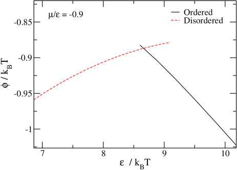
Figure 1: Grand canonical potential of the ordered and disordered phases for $r$=0.32 at $\mu/\epsilon=-0.9$. The order-disorder phase transition occurs at the crossing of the two branches.

Having obtained the transition temperature at $\mu=\mu_{0}$, GDI integration is used to calculate the coexistence lines at different temperatures, as was done for the liquid-vapor equilibria. At low temperatures we used large system sizes $L=64$, otherwise $L=32$.

III.3 Consistency checks

The calculations of the liquid-vapor and order-disorder transitions were checked by performing simulations with two fully independent programs written by two of the coauthors of this paper. In one of the MC codes cluster sampling techniques were included whereas in the the other (control program) only simple single site moves were included. The control code was used to calculate the liquid-vapor and order-disorder transition using thermodynamic integration. These calculations validate both the enhanced sampling techniques and the proper coding of the Wang-Landau and cluster moves in the GCMC/GDI simulations.

The calculation of the order-disorder transition using the control code was carried out using the thermodynamic integration technique described in the previous section, whereas the calculation of the liquid-vapor equilibria by thermodynamic integration is described briefly in what follows.

For the vapor phase, the grand canonical potential was obtained integrating along an isotherm from very low values of the chemical potential (or densities), where the system behaves as an ideal gas, to the chemical potential of interest using:

$$\beta\phi(\mu)=\beta\phi(\mu_{ideal})-\beta\int_{\mu_{ideal}}^{\mu}\eta(\mu^{\prime})d\mu^{\prime}$$ (31)

where $\mu_{ideal}$ represents a value of the chemical potential low enough so that the behavior of the fluid can be considered ideal. The grand canonical potential of the ideal gas can be easily calculated using:

$$\beta\phi(\mu)=-\beta p$$ (32)

and the ideal gas equation to obtain:

$$\beta\phi(\mu_{ideal})=-\eta$$ (33)

The free energy of the liquid was calculated through an integration path starting at the high temperature limit, where the free energy is calculated as in the previous section (Eq.25). The integration was performed in two steps: first, we integrate from infinite temperature to the temperature of interest keeping the chemical potential $\mu$ constant (Eq. 27) and, second, we integrate along an isotherm from $\mu$ to the chemical potential of interest (Eq. 31). As usual we ensure that there are no phase transitions along the chosen thermodynamic path.

Analogously to the calculation of the order-disorder transition the liquid-vapor coexistence is obtained by calculating, at the given temperature, the chemical potential where the grand canonical potentials of the two phases are equal.

All the simulations performed with the control Monte Carlo code considered systems with $L=$24. The results obtained using the two different codes and methodologies are found to be consistent.

IV Results

In Figure 2 we plot the results for the liquid-vapor equilibria, including the estimates for the critical point (these are also given in Table 1). The general trend is as expected from earlier workRusso et al. (2011, 2011); Almarza et al. (2011): As $r$ decreases the critical point is shifted to lower densities and lower temperatures. In addition for $r<1/2$ the LVE is reentrant, with densities of the liquid phase at coexistence decreasing on cooling at low temperatures. The LVE binodals were computed using GDI with system size $L=32$ (i.e. $M=$ 131 072) for $r>0.30$ (except at the lowest temperatures, where $L=64$ ($M=$ 1 048 576) was used to avoid interconversion between the two phases). For $r=0.30$ larger systems, $L=64$, were required to obtain reliable results at all temperatures. In all cases, the GDI fails at sufficiently low temperatures, due to the rapid growth of the typical size of the voids in the (emptying) coexisting liquid as reported previously Almarza et al. (2011). As in other $2AnB$ models Russo et al. (2011, 2011); Almarza et al. (2011); Almarza (2012) the binodal at a given $r$ encloses the binodals at smaller values of $r$.

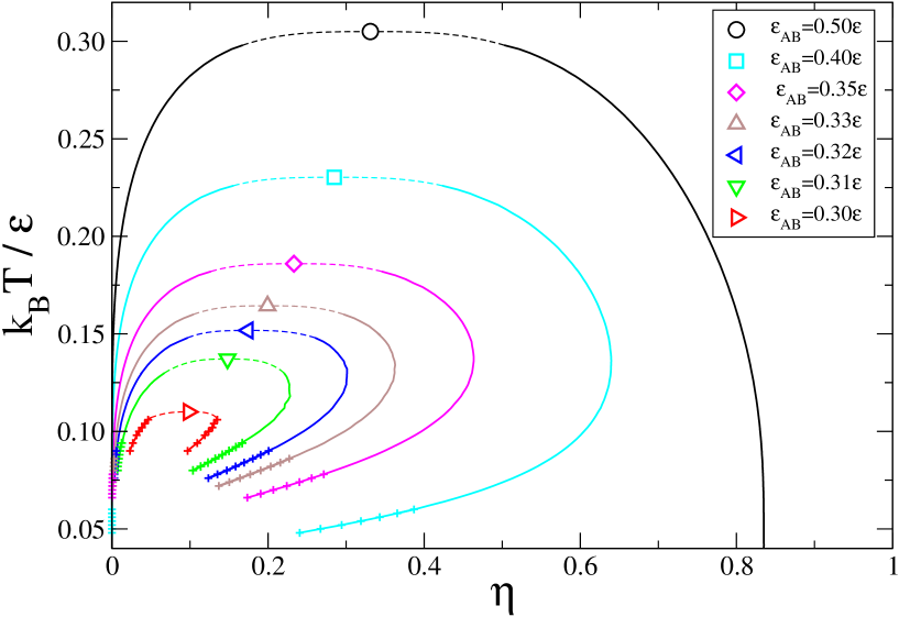
Figure 2: Liquid-vapor binodals, for different $r=\epsilon_{AB}/\epsilon$. Large open symbols mark the critical points. Continuous lines represent GDI results, the points on these lines mark the portions that were computed using larger system sizes ($L=64)$. Dashed lines are included to connect the GDI results with the critical point estimates.

The most remarkable result, however, is the clear evidence of LVE for systems with $r<\frac{1}{3}$. As mentioned in the Introduction, earlier theoretical predictions based on Wertheim’s first-order perturbation theory set the threshold for liquid-vapor coexistence at $r=\frac{1}{3}$ in line with simulation results for $2AnB$ models Russo et al. (2011); Almarza et al. (2011). The finding is also relevant in a wider context, as this threshold was used recently to address the liquid-vapor condensation in other systems that form branched chains at low temperatures, in particular dipolar hard spheresTavares and Teixeira (2011). We will return to this discussion later, after the theoretical analysis described in Sec. V.

Lattice models allow the precise location of not only the liquid-vapor transition, but also the order-disorder transition that occurs at higher densities (the lattice analogue of the fluid-solid transition of off-lattice models). As in the 2D lattice, we find that the order-disorder transition occurs always at a higher density (higher chemical potential), in the temperature range accessible to simulations (see Fig. 3) Almarza et al. (2011).

Interesting scaling features are revealed by plotting the LVE and the order-disorder binodals for different values of $r$ as functions of the scaled temperature, $t=k_{B}T/[(1-2r)\epsilon]$ (see Fig. 3). First, in the limit of full occupancy the order-disorder transitions collapse into a single point. This is an exact result, and the observed collapse is just a check of the consistency and accuracy of our simulation protocols. In addition, the order-disorder transition exhibits a very weak dependence on $r$; i.e. the lines for the order-disorder transition for $r=0.32$, and $r=0.40$ are almost indistinguishable. By contrast, the order-disorder transition of the SARR model ($r=0$), deviates clearly from the previous ones. Finally, as in the T-$\eta$ representation, the binodal for a given $r$ encloses the binodals for lower values of $r$.

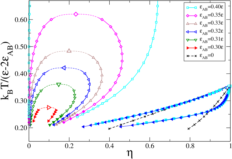
Figure 3: Binodals for the liquid-vapor and order-disorder transitions, for different $r=\epsilon_{AB}/\epsilon$, as functions of a rescaled temperature. Filled symbols mark the portions of the curves that were computed using larger system sizes (L=64).

$r$	$T_{c}^{*}$	$\eta_{c}$	$\mu_{c}$
0.300	$0.1163(9)$	$0.105(4)$	-1.0361(10)
0.305	0.1277(3)	0.1284(10)	-1.0522(4)
0.310	0.1371(4)	0.148(2)	-1.0679(6)
0.320	0.1518(2)	0.175(2)	-1.0961(3)
0.330	0.1644(1)	0.1993(10)	-1.1245(2)
0.350	0.1860(1)	0.2331(2)	-1.1808(2)
0.400	0.2302(1)	0.2848(3)	-1.3228(1)
0.450	0.2689(1)	0.3136(3)	-1.4684(1)
0.500	0.3050(1)	0.3310(2)	-1.6169(1)

Table 1: Estimates of the critical points for different values of $r$

V Wertheim’s theory for $2AnB$ lattice models

The free energy per particle, within Wertheim’s first order perturbation theory, for a homogeneous system of particles with 2 patches of type $A$ and $n$ patches of type $B$ is Tavares et al. (2009, 2009),

$$\beta f=\beta f_{ref}+2(\ln X_{A}-\frac{X_{A}}{2})+n(\ln X_{B}-\frac{X_{B}}{2}),$$ (34)

where $f_{ref}$ is the free energy per particle of the reference system and $X_{\alpha}$ the fraction of unbonded patches of type $\alpha$. The laws of mass action that relate $X_{\alpha}$, the density $\eta$ and the temperature $T$ are (when there are no $BB$ interactions)Tavares et al. (2009, 2009),

$$X_{A}+2\eta\Delta_{AA}X_{A}^{2}+n\eta\Delta_{AB}X_{A}X_{B}=1,$$ (35)

$$X_{B}+2\eta\Delta_{AB}X_{A}X_{B}=1.$$ (36)

As for the $2A2B$ model on the square lattice, the reference system is an ideal lattice gas Almarza et al. (2011), and thus,

$$\beta f_{ref}=\ln\eta+\frac{1-\eta}{\eta}\ln(1-\eta).$$ (37)

The $\Delta_{\alpha\beta}$ are integrals of the Mayer functions of two patches $\alpha$ and $\beta$ on two different particles, over their positions and orientations, weighted by the pair distribution function of the reference system. In continuous systems the $\Delta_{\alpha\beta}$ are calculated from,

$$\Delta_{\alpha\beta}=\frac{1}{V(4\pi)^{2}}\int d\vec{r}_{1}d\vec{r}_{2}\int d\vec{\omega}_{1}d\vec{\omega}_{2}g_{ref}(\vec{r}_{1},\vec{r}_{2})f_{\alpha\beta}(\vec{r}_{1},\vec{r}_{2},\vec{\omega}_{1},\vec{\omega}_{2}),$$ (38)

where $\alpha$ is a particular patch on particle 1 and $\beta$ is a particular patch on particle 2, $\vec{r}_{i}$ refers to the position of particle $i$ and $\vec{\omega}_{i}$ to the orientation of the particular patch on particle $i$ that is being considered; the factor $1/(4\pi)^{2}$ takes into account that there is no preferred orientation for the position of the patches on the particles surfaces. Finally, $f_{\alpha\beta}(\vec{r}_{1},\vec{r}_{2},\vec{\omega}_{1},\vec{\omega}_{2})$ is the Mayer function of the interaction potential between patches $\alpha$ and $\beta$, and $g_{ref}(\vec{r}_{1},\vec{r}_{2})$ is the pair correlation function of the reference systemTavares et al. (2009, 2009).

The calculation of $\Delta_{\alpha\beta}$ on a lattice with coordination number $z$ and particles with $z$ patches, (as in the $2AnB$ models considered here and in Almarza et al. (2011)) is carried out by discretizing Eq. 38,

$$\Delta_{\alpha\beta}=\frac{1}{Mz^{2}}\sum_{i_{1}=1}^{M}\sum_{i_{2}=1}^{M}\sum_{l_{1}=1}^{z}\sum_{l_{2}=1}^{z}f_{\alpha\beta}(i_{1},i_{2},l_{1},l_{2})g_{ref}(i_{1},i_{2}).$$ (39)

Here the patch $\alpha$ is on particle $1$ and the patch $\beta$ on particle $2$; $i_{1}$ and $i_{2}$ represent the positions of particles 1 and 2, respectively; $M$ is the total number of lattice sites (equivalent to the volume); the factor $1/z^{2}$ accounts for the fact that there is no preferred orientation for the patches, as $z$ is also the number of different orientations of a given patch. The integers $l_{1}$ and $l_{2}$ run over the possible orientations of each patch. For the potential described in Sec. II, the Mayer function $f_{\alpha\beta}(i_{1},i_{2},l_{1},l_{2})$ is non zero when: (a) $1$ and $2$ are NN and (b) $l_{1}$ and $l_{2}$ are such that patches $\alpha$ and $\beta$ are properly oriented along the interparticle direction. Using $g_{ref}=1$, Eq. 39 is simplified to,

$$\Delta_{\alpha\beta}=v_{\alpha\beta}\left[\exp(\beta\epsilon_{\alpha\beta})-1\right],$$ (40)

where $v_{\alpha\beta}$, the volume of a bond between patches of type $\alpha$ and $\beta$, is

$$v_{\alpha\beta}=1/z.$$ (41)

For the $2AnB$ models under consideration, the bonding volume $v_{\alpha\beta}$ is independent of the types of patches and is related to the number of $B$ patches $z=n+2$.

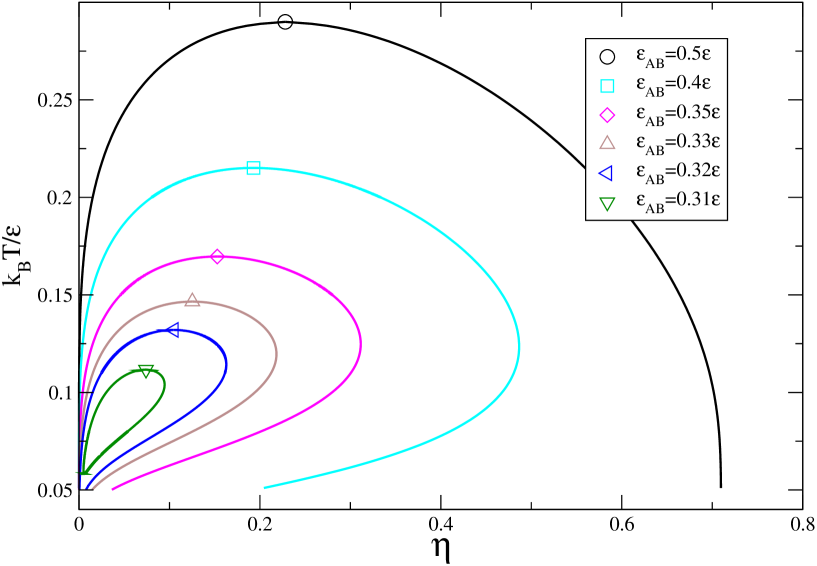
Figure 4: Liquid-vapor binodals, for different $r=\epsilon_{AB}/\epsilon$, calculated using Wertheim’s first order perturbation theory. Larger critical temperatures correspond to larger values of $r$.

The liquid-vapor binodals calculated using Wertheim’s theory, for models with $n=10$, i.e. the models simulated in Sec. IV, are plotted in Figure 4, for several $r$. As expected Almarza et al. (2011); Russo et al. (2011, 2011), Wertheim’s theory predicts, in agreement with the simulation results, the reentrance of the liquid binodal for $r<\frac{1}{2}$. The phase diagrams were calculated for models with $r>0.305$: below this value no liquid-vapor coexistence was found.

To clarify this surprising behavior, in view of previous results Tavares et al. (2009, 2009); Russo et al. (2011, 2011); Almarza et al. (2011), we solved the set of equations, $\left(\frac{\partial^{2}f}{\partial\eta^{2}}\right)_{T}=0$ and $\left(\frac{\partial^{3}f}{\partial\eta^{3}}\right)_{T}=0$, which determine the critical density and temperature as a function of the parameters of the lattice $2AnB$ model, namely $r$ and $n$ (or the coordination number $z$). The results for $n=2$, $n=4$, $n=6$ and $n=10$ (corresponding to square Almarza et al. (2011), triangular or simple cubic, body centered cubic, and face centered cubic lattices, respectively) are plotted in Figs. 5 and 6.

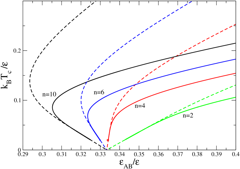
Figure 5: Critical temperature as a function of $r\equiv\epsilon_{AB}/\epsilon$, for several values of $n$. Full lines: critical temperature calculated from Wertheim’s theory Eq. 34; dashed lines: critical temperature calculated from the asymptotic expansion of Wertheim’s theory, Eqs. (43) and (44).

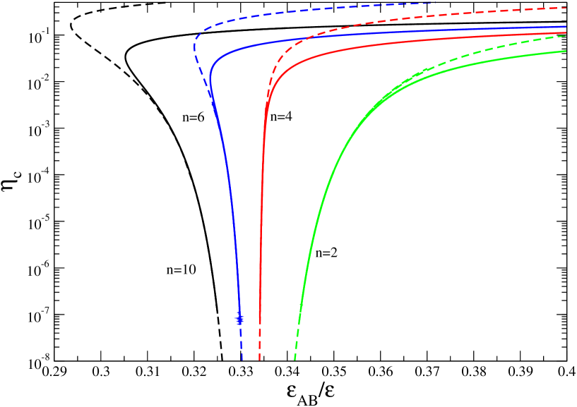
Figure 6: Critical density as a function of $r$ for several values of $n$. Full lines: critical density calculated from Wertheim’s theory Eq. 34; dashed lines: critical temperature calculated from the asymptotic expansion of Wertheim’s theory, Eqs. (43), (44) and (45).

The results reveal that Wertheim’s theory predicts a phase behavior that is strongly dependent on the values of $n$ and $r$. For $n<4$ we recover the threshold reported earlier: no critical point for $r<\frac{1}{3}$ and one critical point otherwise. For larger $n$, however, three distinct regimes are possible depending on the value of $r$: one critical point for $r>\frac{1}{3}$, no critical point for $r$ less than a threshold $r_{m}$ ($<\frac{1}{3}$) and two critical points for the range of $r$ between this threshold and $\frac{1}{3}$.

A deeper understanding of these results, which contrast with the simpler picture reported earlier Tavares et al. (2009, 2009); Russo et al. (2011, 2011); Almarza et al. (2011), is obtained through the asymptotic expansion of the free energy Eq. 34, in the limit of strong $AA$ bonding (i.e $X_{A}\approx 0$) and low densities Tavares et al. (2009, 2009); Russo et al. (2011, 2011). Using this expansion we find for the pressure $p$,

$$\beta p=\frac{\eta^{\frac{1}{2}}}{\sqrt{2\Delta_{AA}}}-\frac{n\Delta_{AB}}{\sqrt{2\Delta_{AA}}}\eta^{\frac{3}{2}}+B_{2}\eta^{2},$$ (42)

where $B_{2}$ is the second virial coefficient of the reference system ($B_{2}=1/2$ for the ideal lattice gas). Using Eq. 42 the critical temperature $T_{c}$ is found to satisfy,

$$G(\epsilon_{AB},T_{c})\equiv\frac{\left[\exp\left(\frac{\epsilon_{AB}}{k_{B}T_{c}}\right)-1\right]^{3}}{\exp\left(\frac{\epsilon}{k_{B}T_{c}}\right)-1}=C,$$ (43)

where $C=\frac{8B_{2}^{2}v_{AA}}{(nv_{AB})^{3}}$. For the $2AnB$ models under consideration, the constant $C$ may be evaluated using Eq. 41 and $B_{2}=1/2$,

$$C=\frac{2(n+2)^{2}}{n^{3}}.$$ (44)

The asymptotic critical density $\eta_{c}$ is then given by,

$$\eta_{c}=\frac{1}{n\Delta_{AB,c}},$$ (45)

where $\Delta_{AB,c}$ is the value of $\Delta_{AB}$ at $T=T_{c}$. In Figures 5 and 6 the asymptotic critical temperature and density are plotted as functions of $r$ for several values of $n$. As expected, the asymptotic results describe those of the full theory at low temperatures, but qualitative agreement is obtained at intermediate temperatures. Thus, the phase behavior of the $2AnB$ model can be described by analyzing Eq. 43.

For $r>\frac{1}{3}$ the function $G(\epsilon_{AB},T_{c})$ is a monotonic decreasing function of $T_{c}$, with limits $\lim_{T_{c}\to 0}=\infty$ and $\lim_{T_{c}\to\infty}=0$. However, for $r<\frac{1}{3}$, this function has a maximum which decreases with decreasing $r$; is limited by $0<G(\epsilon_{AB},T_{c})<1$ and vanishes in the limits, $\lim_{T_{c}\to 0}=0$ and $\lim_{T_{c}\to\infty}=0$. The analysis of the critical behavior of $2AnB$ models is done most simply by considering the cases $C>1$ and $C<1$ (which correspond, Eq.43, to $n\leq 4$ and $n>4$, respectively, for integer values of $n$).

• If $r>\frac{1}{3}$, Eq. 43 has a unique solution, and therefore, there is a single critical point with critical temperature,

  $$T_{c}\approx\frac{3r-1}{\ln C}.$$ (46)

  If $r<\frac{1}{3}$ then $G(\epsilon_{AB},T_{c})<1$ and Eq. 43 has no solution. Therefore, there is no critical point.

  This is the case considered in previous work Tavares et al. (2009, 2009); Russo et al. (2011, 2011), as the models analyzed previously have $C>1$.

• If $r>\frac{1}{3}$, Eq. 43 has one solution and there is a single critical point. If $r<\frac{1}{3}$, we define $r_{m}$ as the value of $r$ where the maximum of $G$, $G_{max}$, is equal to $C$: $G_{max}(r_{m},T_{c})=C$. Then, two cases have to be distinguished: If $r_{m}<r<\frac{1}{3}$, $G_{max}(\epsilon_{AB},T_{c})>C$, and Eq. 43 has two solutions; therefore, there are two critical points; If $r<r_{m}$, Eq. 43 has no solutions, and there is no critical point.

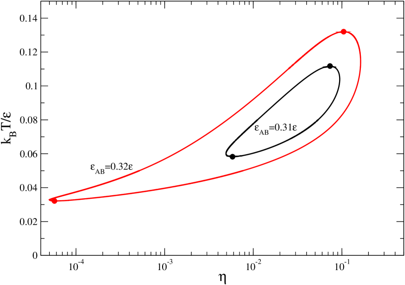
Figure 7: Phase diagrams with two critical points, for $n=10$ and two values of $r<1/3$, calculated using Wertheim’s theory Eq. 34. The circles represent the location of the critical points. These binodals are the same as those of figure 4 for the indicated values of $r=\epsilon_{AB}/\epsilon$, but are represented in a logarithmic scale in the density and extended to lower temperatures, to put highlight the lower critical points.

In Figure 7 we plot a phase diagram with two critical points, for models with $n=10$, and $r=0.31$ and $0.32$.

The liquid vapor coexistence of these models is between a low density, high energy and high entropy phase, formed by short chains, and a high density, low energy and low entropy phase (network liquid) formed by long chains connected by $AB$ bonds, or junctions Russo et al. (2011). It has been shown Russo et al. (2011) that this coexistence is only possible when a decrease in the entropy of chains (or $AA$ bonds) upon condensation, is balanced by an increase in the entropy associated with the junctions (or $AB$ bonds). For systems with $C>1$ and $r<\frac{1}{3}$, the increase in the entropy of the junctions is no longer sufficient to balance the loss in the entropy of the chains Russo et al. (2011).

Systems with $C<1$ have not been discussed earlier as the continuum Russo et al. (2011); Tavares et al. (2009) and the lattice Almarza et al. (2011) models investigated previously belong to the class $C>1$. The $2A10B$ lattice model investigated in this paper belongs to the class $C<1$ and thus exhibits different critical behavior. In these models the balance of entropies may occur at values of $r<\frac{1}{3}$. This may be rationalized by considering the physical meaning of $C$. The entropy of one bond is the logarithm of the volume available (on one particle) to form that bond Sciortino et al. (2007). Then, $\ln C=\ln(\frac{2v_{AA}}{2B_{2}})-3\ln(\frac{nv_{AB}}{2B_{2}})$ is the difference between the entropy of one $AA$ bond and (three times) the entropy of one $AB$ bond. For the $2AnB$ model $\ln C=\ln(\frac{2}{n+2})-3\ln(\frac{n}{n+2})$, and as $n$ increases so does the entropy of the $AB$ bonds. Therefore, when $C<1$ the entropy of junction formation increases, in such way that it can balance the decrease of entropy of the chains, for values of $r<\frac{1}{3}$.

VI Discussion of the results

Despite the challenges posed by the simulations of the phase diagram of empty fluids at low temperatures, the results for the $2A10B$ lattice model confirm the features of the LVE reported for 3D off-lattice Russo et al. (2011, 2011) and 2D lattice $2AnB$ Almarza et al. (2011) models. The variation of the critical densities and temperatures with $r$ follow the expected behavior Russo et al. (2011, 2011); Almarza et al. (2011). In addition, we computed the order-disorder transition that occurs at higher densities, confirming that the low density liquid phase is thermodynamically stable as in the 2D model Almarza et al. (2011).

We have, however, found an unexpected result: LVE for systems with $r<\frac{1}{3}$, by contrast to previous simulation results and the theoretical analyses based on Wertheim’s theory Tavares et al. (2009, 2009); Russo et al. (2011, 2011) as well as an earlier prediction based on a hierarchical theory of network fluids Tulsty and Safran (2000). The threshold $r=\frac{1}{3}$ results from an asymptotic expansion of Wertheim’s first-order perturbation theory, which assumes that the constant $\ln C$ is positive as described in Sec. V. This is certainly the case for $2AnB$ models on and off-lattice if the number of $B$ patches is not too large. For lattice models, however, the bonding volume compatible with a single bond per patch assumed by Wertheim’s theory is much larger than in similar off-lattice models (the exclusion of the second particle being guaranteed by the lattice structure) and thus $\ln C$ can become negative. In this case, Wertheim’s first-order perturbation theory and its asymptotic expansion in the limit of strong $AA$ bonding predicts indeed the possibility of LVE for $r<\frac{1}{3}$. The theoretical analysis also predicts that in this regime the reentrancy of the liquid-vapor binodal is extreme in the sense that the system exhibits a low temperature critical point. The theoretical prediction is then that when $\ln C$ is negative (large values of $nv_{AB}$) $2AnB$ models exhibit a closed miscibility loop in a range of $r<\frac{1}{3}$. There is also a new threshold, which depends on the number of $B$ patches, below which the closed miscibility loop vanishes and where there is no condensation.

Previous simulation results on and off lattice were compatible with the original $\frac{1}{3}$ threshold, and in line with the theoretical results for positive $\ln C$ Russo et al. (2011, 2011); Almarza et al. (2011).

The closed miscibility loop predicted for systems with negative $\ln C$ has not been confirmed by simulations, since the density and temperatures at which they occur are beyond the current simulation techniques.

In related work, a $2A4B$ 2D lattice model with $\frac{1}{2}>r>\frac{1}{3}$ was shown to exhibit the usual reentrant behavior when the position of the $A$ patches prevents the formation of rings, a closed miscibility loop when the orientation of the $A$ patches promotes relatively large rings and no phase coexistence when the orientation of the $A$ patches promotes short rings Almarza (2012). The topology of the phase diagram of this $2B4A$ lattice model with $r>\frac{1}{3}$ changes as the orientation of the $A$ patches changes (promoting the formation of rings) in a fashion that resembles the behavior of the $2A10B$ model as $r$ decreases. Although the physics may be related a detailed, quantitative and qualitative, analysis is required in order to investigate the analogies in the driving mechanisms of the different transitions.

Along these lines, recent work for a model with $A$ patches addressed quantitavely the competition between ring and chain formation, within an extension of Wertheim’s first-order perturbation theory and by simulation Tavares et al. (2012). An extension of this approach to $2AnB$ models and the calculation of the corresponding phase diagrams is a challenging task that will be addressed in future work. Likewise new simulation algorithms will be developed to confirm the presence of closed miscibility loops, in systems with no rings, as predicted by Wertheim’s first-order perturbation theory as well as the new thresholds, $r<\frac{1}{3}$, for models with negative $\ln C$.

The degree of universality of the new thresholds is also an important open question, in general, and in the context of the condensation of dipolar hard-spheres.

VII Appendix: Cluster algorithms

In this appendix the cluster algorithms that we used in the Grand Canonical ensemble simulations of the GDI method are described. The two cluster moves defined here do not include, in general, the whole set of sites of the lattice, but only those sites with two of the possible values of $s_{i}$. In practical terms we can classify the cluster moves in two types: Moves that change the number of occupied sites: Cluster N-sampling, and moves in which the orientation of some of the sites can change: Cluster Orientation-sampling. A full derivation of the procedures might be cumbersome, so we will just include the steps and considerations required to understand the recipe of the algorithms.

VII.1 Cluster N-Sampling

In these moves we consider only empty sites and occupied sites with one (chosen at random) of the six possible orientations, $s_{r}$. These sites are named active sites. We classify as passive (or blocked) those sites $k$ with $s_{k}\neq s_{r}$ and $s_{k}\neq 0$. Passive sites are not modified in these moves, and play the role of an external field. Taking into account the values of the interaction parameters, and in particular that $\epsilon_{BB}=0$, one occupied active site interacts with another occupied active site if (and only if) both sites are NN in the $s_{r}$ direction. Using this definition of active sites the system can be equivalently seen as a collection of one dimensional rows of sites (with PBC), i.e. 1D lattice gas models under the influence of external fields. The terms of the Grand Canonical Hamiltonian that deppend on the active sites can be written as:

$${\cal H}_{A}=-\epsilon\sum_{<ij>_{s_{r}}}^{A}\rho_{i}\rho_{j}-\sum_{i}^{A}\rho_{i}\left[\mu+\epsilon rN_{1}(i)+\epsilon rN_{2}(i)\right]$$ (47)

where the first sum on the right hand side is carried out exclusively over pairs of active sites which are NN along the direction $s_{r}$. The second sum includes only active sites. The variables $\rho_{i}$ take the values $0$ for empty sites and $1$ for occupied sites. $N_{1}(i)$ is the number of $A$ patches of the site $i$ that points to a NN passive site, and $N_{2}(i)$ is the number of $A$ patches belonging to a NN passive site of $i$ that point to site $i$. Through the change of variables $\rho_{i}=(1+\sigma_{i})/2$; ${\cal H}_{A}$, may be written as an Ising-like Hamiltonian:

$${\cal H}_{A}-{\cal H}_{0}=-\frac{\epsilon}{4}\sum_{<ij>_{s_{r}}}^{A}\sigma_{i}\sigma_{j}-\frac{\mu+\epsilon}{2}\sum_{i}^{A}\sigma_{i}-\sum_{i}^{A}\sigma_{i}\left[\frac{\epsilon r}{2}N_{2}(i)+\left(\frac{\epsilon r}{2}-\frac{\epsilon}{4}\right)N_{1}(i)\right];$$ (48)

where ${\cal H}_{0}$ includes the terms that do not depend on the state of the active sites. The new variables $\sigma_{i}$ can take the values $\pm 1$. On the right hand site of Eq. (48) the first term is the Ising-like interaction, the second plays the role of a global external field, and the last one includes the local external fields that depend on the configuration of the passive sites.

Within this representation of the interactions of the active sites, it is straighforward to build up a cluster algorithm following the Swendsen-Wang procedureSwendsen and Wang (1987) and its extensions in the presence of external fields Landau and Binder (2005). The recipe of such an algorithm goes as follows: (1) Generate bonds between pairs, $\{i,j\}$, of active sites which are NN in the $s_{r}$ direction, and that fulfill $s_{i}=s_{j}$ with probability:

$$B_{ij}=1-\exp\left[-\epsilon/(2k_{B}T)\right];$$ (49)

(2) Consider separately each one of the clusters of active sites defined by the previous bonds. Taking into account the effect of the external fields given in Eq.(48), the new configuration is generated by assigning to all the lattice sites in the cluster either $s=0$ (i.e. $\sigma=-1$); or $s=s_{r}$ (i.e. $\sigma=1$) with probabilities $A(c,s)$ (where $c$ is the index for the $c$-th cluster) fulfilling:

$$\frac{A(c,s_{r})}{A(c,0)}=\exp\left\{\frac{\mu+\epsilon}{k_{B}T}n_{i}(c)+\frac{(r-1/2)\epsilon{\cal N}_{1}(c)+\epsilon r{\cal N}_{2}(c)}{k_{B}T}\right\};$$ (50)

where $n_{i}(c)$ is the number of lattice sites in the cluster $c$, ${\cal N}_{1}(c)$ is the number of $A$ patches in the cluster $c$ that point to a NN blocked site, and ${\cal N}_{2}(c)$ is the number of A patches lying at blocked sites that point to a NN site in the cluster $c$.

VII.2 Cluster orientation sampling

In these cluster moves two of the possible orientations, $s_{a}$, $s_{b}$, of the particles are chosen as active directions, whereas the remaining four directions and the empty sites are classified as passive (or blocked) directions. In the moves only active sites can modify their states (from $s_{a}$ to $s_{b}$ and vice versa). Therefore the number of occupied sites will remain constant. Notice that the interaction between two active sites that are NN through a passive direction is equal to $\epsilon_{BB}$ independently of their respective orientations. In addition, the interaction between two NN sites, one being active and the other passive can be modified in these moves only if they are NN through an active direction.

From these features of the interaction potential, it follows that the only relevant interactions in the proposed restricted sampling are those that take place between NN sites through the active directions. As a consequence the system can be treated as a set of independent layers with the topology of the square lattice (defined by the two active orientations), that can contain active sites and two types of passive sites: empty and blocked sites. The relevant terms of the potential energy on each layer take the form:

$${\cal H}_{A}=-\epsilon\sum_{<ij>}\delta_{s_{i},s_{j}}\delta_{s_{i},\alpha_{ij}}-\epsilon r\sum_{[ik]}\delta_{s_{i},\alpha_{ik}}\left(1-\delta_{s_{k},0}\right);$$ (51)

where the $\delta$’s represent Kronecker delta functions, $<ij>$ indicates pairs of NN active sites on the square lattice; $[ik]$ stands for pairs of NN with $i$ and $k$ being respectively an active and a passive site; and $\alpha_{lm}$ is the index of the direction ${\vec{r}}_{lm}$.

Now, we describe the strategy to generate the cluster algorithm. In previous papers Almarza et al. (2010, 2011) we showed how the lattice patchy models defined on the square lattice at full occupancy can be mapped onto the two-dimensional lattice gas model. It can be shown that it is also possible to carry out a mapping when some of the sites are blocked, the main difference being that the effect of the blocked sites enters as a local external field. Almarza et al. (2012) This mapping can be obtained through the plaquette procedures used in previous papers. Taking into account plaquettes of four sitesAlmarza and Noya (2011); Almarza et al. (2010), and defining on each plaquette $h_{A}$ as the sum of the potential energy contributions involving at least one active particle, it can be shown that $h_{A}$ can be written in terms of a Potts-like interaction as:

$$h_{A}=h_{0}-K\sum_{<ij>}^{p}\delta_{s_{i},s_{j}}+K_{1}\sum_{[ik]}^{p}\delta_{s_{i},\alpha_{ik}}\left(1-\delta_{s_{k},0}\right)+K_{10}\sum_{[ik]}^{p}\delta_{s_{i},\alpha_{ik}}\delta_{s_{k},0};$$ (52)

where the superscript $p$ over the sums indicates that only interactions between sites belonging to the plaquette are considered, $h_{0}$ is just an additive constant which deppends on the configuration of the passive sites in the plaquette, but not on the state of the active sites, and finally $K$, $K_{10}$ and $K_{0}$ deppend only on the energy parameters of the patchy model: $\epsilon$ and $r$. Since ${\cal H}_{A}$ can be written as one half of the sum of the plaquettes energies $h_{A}$, we find

$${\cal H}_{A}-H_{0}=-K\sum_{<ij>}\delta_{s_{i},s_{j}}+K_{1}\sum_{[ik]}\delta_{s_{i},\alpha_{ik}}\left(1-\delta_{s_{k},0}\right)+K_{10}\sum_{[ik]}\delta_{s_{i},\alpha_{ik}}\delta_{s_{k},0}$$ (53)

where $H_{0}$ is an additive constant which does not deppend on the configuration of the active sites, $K\equiv(1/2-r)\epsilon$, $K_{1}=K$, and $K_{10}=\epsilon/2$. On the right and side of Eq. (53) : the first term is a Potts $q=2$ interaction; the second term includes the effective interaction of active sites with their NN occupied passive sites (on the square lattice), whereas the last term represents the effective interactions of active sites with their NN passive empty sites (on the square lattice). The last two terms can be seen, as before, as local external fields.

Once the interaction between active sites has been described in terms of the Potts model, it is straighforward to use the same strategy described for the cluster N-sampling. Following Ref. (Landau and Binder, 2005), the algorithm recipe is: Pairs of active sites, $(i,j)$ being NN (on the chosen square lattice) that fulfill $s_{i}=s_{j}$ are bonded with probability:

$$B_{ij}=1-\exp\left[-K/(k_{B}T)\right].$$ (54)

These bonds define clusters of active sites; and the orientation of each of the clusters in the new configuration is chosen from the active directions: $s_{\alpha}=s_{a},s_{b}$; with probabilities:

$$A(c,s_{\alpha})\propto\exp\left[-N^{(0)}(s_{\alpha})\frac{\epsilon}{2k_{B}T}-N^{(1)}(s_{\alpha})\frac{(1/2-r)\epsilon}{k_{B}T}\right];$$ (55)

where $N^{(0)}(s_{\alpha})$ is the number of A patches belonging to the cluster that point to empty blocked NN sites when the particles of the cluster are oriented in direction $s_{\alpha}$, and $N^{(1)}(s_{\alpha})$ is the number of A patches belonging to the cluster pointing to occupied blocked NN sites when the cluster is oriented in direction $s_{\alpha}$.

References

- Glotzer and Solomon (2005) S. C. Glotzer and M. J. Solomon, Nat. Mater., 6, 557 (2005).
- Pawar and Kretzschmar (2010) A. B. Pawar and I. Kretzschmar, Macromol. Rapid Commun., 31, 150 (2010).
- Bianchi et al. (2011) E. Bianchi, R. Blaak, and C. Likos, Phys. Chem. Chem. Phys., 13, 6397 (2011).
- Tavares et al. (2009) J. M. Tavares, P. I. C. Teixeira, and M. M. Telo da Gama, Phys. Rev. E, 80, 021506 (2009a).
- Tavares et al. (2009) J. M. Tavares, P. I. C. Teixeira, and M. M. Telo da Gama, Molec. Phys., 107, 453 (2009b).
- Russo et al. (2011) J. Russo, J. M. Tavares, P. I. C. Teixeira, M. M. Telo da Gama, and F. Sciortino, J. Chem. Phys., 135, 034501 (2011a).
- Russo et al. (2011) J. Russo, J. M. Tavares, P. I. C. Teixeira, M. M. Telo da Gama, and F. Sciortino, Phys. Rev. Lett., 106, 085703 (2011b).
- Tavares et al. (2010) J. M. Tavares, P. I. C. Teixeira, M. M. Telo da Gama, and F. Sciortino, J. Chem. Phys., 132, 234502 (2010).
- Wertheim (1984) M. S. Wertheim, J. Stat. Phys., 35, 19 (1984a).
- Wertheim (1984) M. S. Wertheim, J. Stat. Phys., 35, 35 (1984b).
- Wertheim (1986) M. S. Wertheim, J. Stat. Phys., 42, 459 (1986a).
- Wertheim (1986) M. S. Wertheim, J. Stat. Phys., 42, 477 (1986b).
- Tulsty and Safran (2000) T. Tulsty and S. A. Safran, Science, 290, 1328 (2000).
- Almarza et al. (2011) N. G. Almarza, J. M. Tavares, M. Simões, and M. M. Telo da Gama, J. Chem. Phys., 135, 174903 (2011).
- Bianchi et al. (2006) E. Bianchi, J. Largo, P. Tartaglia, E. Zaccarelli, and F. Sciortino, Phys. Rev. Lett., 97, 168301 (2006).
- Tavares and Teixeira (2011) J. M. Tavares and P. I. C. Teixeira, Molec. Phys., 109, 1077 (2011).
- Rovigatti et al. (2011) L. Rovigatti, J. Russo, and F. Sciortino, Phys. Rev. Lett., 107, 237801 (2011).
- Almarza (2012) N. G. Almarza, Phys. Rev. E, 86, 030101(R) (2012).
- Lomba et al. (2005) E. Lomba, C. Martín, N. G. Almarza, and F. Lado, Phys. Rev. E, 71, 046132 (2005).
- Ganzenmüller and Camp (2007) G. Ganzenmüller and P. J. Camp, J. Chem. Phys., 127, 154504 (2007).
- Almarza et al. (2008) N. G. Almarza, E. Lomba, C. Martín, and A. Gallardo, J. Chem. Phys., 129, 234504 (2008).
- Almarza et al. (2009) N. G. Almarza, Capitán, J. A. Cuesta, and E. Lomba, J. Chem. Phys., 131, 124506 (2009).
- Pérez-Pellitero et al. (2006) J. Pérez-Pellitero, P. Ungerer, G. Orkoulas, and A. D. Mackie, J. Chem. Phys., 125, 054515 (2006).
- Almarza and Noya (2011) N. G. Almarza and E. G. Noya, Molec. Phys., 109, 65 (2011).
- Høye et al. (2009) J. S. Høye, E. Lomba, and N. G. Almarza, Molec. Phys., 107, 321 (2009).
- Wang and Landau (2001) F. Wang and D. P. Landau, Phys. Rev. Lett., 86, 2050 (2001a).
- Wang and Landau (2001) F. Wang and D. P. Landau, Phys. Rev. E, 64, 056101 (2001b).
- Allen and Tildesley (1987) M. P. Allen and D. J. Tildesley, Computer Simulation of Liquids (Oxford University Press, 1987).
- Wilding (1995) N. B. Wilding, Phys. Rev. E, 52, 602 (1995).
- Blöte et al. (1995) H. W. J. Blöte, E. Luijten, and J. R. Heringa, J. Phys. A: Math. Gen., 28, 6289 (1995).
- Kofke (1993) D. A. Kofke, Mol. Phys., 78, 1331 (1993).
- Almarza et al. (2012) N. G. Almarza, J. M. Tavares, and M. M. Telo da Gama, J. Chem. Phys., 137, 074901 (2012).
- Hansen and Verlet (1969) J. P. Hansen and L. Verlet, Phys. Rev., 184, 151 (1969).
- Sciortino et al. (2007) F. Sciortino, E. Bianchi, J. F. Douglas, and P. Tartaglia, J. Chem. Phys., 126, 194903 (2007).
- Tavares et al. (2012) J. M. Tavares, L. Rovigatti, and F. Sciortino, J. Chem. Phys., 137, 044901 (2012).
- Swendsen and Wang (1987) R. H. Swendsen and J. S. Wang, Phys. Rev. Lett., 58, 86 (1987).
- Landau and Binder (2005) D. P. Landau and K. Binder, A Guide to Monte Carlo Simulations in Statistical Physics, 2nd edition (Cambridge University Press, 2005).
- Almarza et al. (2010) N. G. Almarza, J. M. Tavares, and M. M. Telo da Gama, Phys. Rev. E, 82, 061117 (2010).