Phase separation of antiferromagnetic ground states in systems with imperfect nesting

Abstract

We analyze the phase diagram for a system of weakly-coupled electrons having an electron- and a hole-band with imperfect nesting. Namely, both bands have spherical Fermi surfaces, but their radii are slightly different, with a mismatch proportional to the doping. Such a model is used to describe: the antiferromagnetism of chromium and its alloys, pnictides, AA-stacked graphene bilayers, as well as other systems. Here we show that the uniform ground state of this model is unstable with respect to electronic phase separation in a wide range of model parameters. Physically, this instability occurs due to the competition between commensurate and incommensurate antiferromagnetic states and could be of importance for other models with imperfect nesting.

I Introduction

Electron models having a band structure with imperfect nesting are employed to analyze properties of several physical systems. For example, such models are used to describe: the antiferromagnetism (AFM) in Cr and its alloys RiceMod ; Review88 , superconducting iron pnictides and iron chalcogenides singh_physC2009 ; vorontsov_prb2010 ; gorkov_teit_prb2010 ; dagotto2012 , AA-stacked graphene bilayers our_aa_paper ; our_aa_phasep_preprint , and other systems gorkov_mnatzakov .

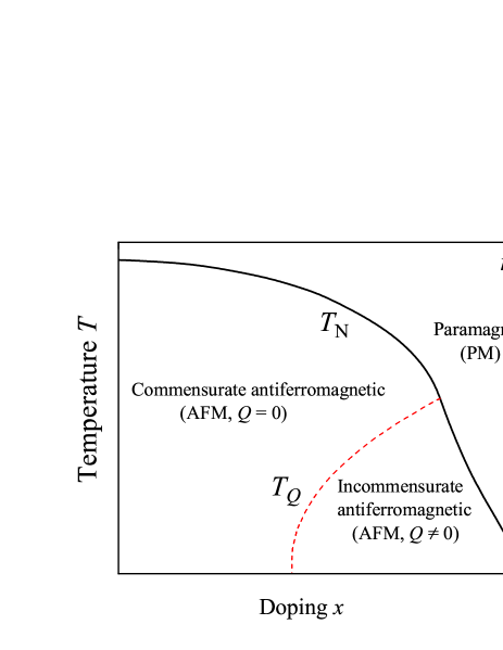
Figure 1: (Color online) A typical phase diagram of a magnetic system with imperfect nesting in the $(x,T)$-plane, where $x$ is the doping and $T$ is the temperature. The solid (black) curve represents the Néel temperature $T_{\textrm{N}}(x)$ separating the paramagnetic (PM) and the antiferromagnetic (AFM) states. The dashed (red) curve is the boundary $T_{Q}(x)$ between the commensurate ($Q=0$) and incommensurate ($Q\neq 0$) AFM states. This phase diagram is constructed for a finite density of states of non-magnetic electrons ($n\neq 0$, see the text).

Postulating a spatially-homogeneous AFM ground state, a phase diagram for models with imperfect nesting can be constructed. A typical $(x,T)$ phase diagram is schematically shown in Fig. 1. This diagram is split into three areas. The first is the paramagnetic state at temperatures higher than the Néel temperature $T_{\textrm{N}}(x)$. If $T<T_{\textrm{N}}(x)$ the system is in one of two magnetically-ordered states. The commensurate AFM state exists at relatively low doping (where the nesting is good) and higher temperatures, while the incommensurate AFM state appears at higher doping and lower temperatures (see Fig. 1). Of course, in the commensurate phase the spatial variation of the order parameter is commensurate with the crystal lattice period. As for the incommensurate AFM, its structure is characterized by the wave vector ${\bf Q}(x,T)$. This ${\bf Q}$ quantifies the smooth variation of the AFM order parameter in real space over distances much longer than the lattice spacing. Since ${\bf Q}$ is zero in the commensurate phase, the condition ${\bf Q}(x,T)=0$ defines the boundary temperature $T_{Q}(x)$ between the commensurate and incommensurate AFM.

The phase diagram in Fig. 1 was obtained RiceMod assuming that the ground state of the system is uniform. However, this assumption is not necessary valid: below we demonstrate that, depending on the doping and the temperature, the homogeneous state may be unstable. To prove this we calculate the chemical potential $\mu(x,T)$ for the model Hamiltonian of the itinerant AFM proposed by Rice RiceMod . We observe that $\partial\mu/\partial x$ is negative in a considerable portion of the $(x,T)$-plane. The homogeneous state compressibility, therefore, is negative, and such state is unstable with respect to electronic phase separation.

It is not difficult to check a particular model for the phase separation instability: an interval of dopings where free energy is a concave function of doping is the signature of phase separation. Yet, the phenomenon is sometimes overlooked due to the fact that other important properties of a homogeneous state bear little or no signature of the underlying instability. For example, the single-particle gap of a homogeneous state may be a smooth decreasing function of doping our_aa_phasep_preprint , and rises no suspicion that, in fact, the state is unstable. Thus, a separate assessment of the thermodynamic stability is required.

In this study we will restrict ourselves to the Rice model. However, the discussed mechanism for the phase separation could be of importance to other systems with imperfect nesting. For example, there are experimental indications that pnictides and chalcogenides may experience such a phenomenon in some regions of doping and temperature Fe_separation_experiment .

This paper is organized as follows. In Sec. II we introduce the model Hamiltonian and derive the equations describing the homogeneous states of the model. The instability of the homogeneous states are presented in Sec. III. The discussion and conclusions can be found in Sec. IV.

II Main equations of the model

We study the model proposed by Rice RiceMod to describe the incommensurate antiferromagnetism in chromium (see also the review in Ref. Review88, ). We mostly adhere to the notation of Ref. RiceMod, . However, to comply with modern conventions, some changes will be introduced. We also correct some misprints present in the latter reference.

The model band structure has one spherical electron pocket and one spherical hole pocket with different radii (imperfect nesting), as well as other band or bands, which do not participate in the magnetic ordering. All interactions are ignored except the repulsion between the electrons in the ordering pockets.

The system we study is three-dimensional. Its Hamiltonian has the form

$$\hat{H}\!=\!\!\sum_{\mathbf{k},\sigma\atop\alpha=a,b,c}\epsilon^{\alpha}(\mathbf{k})n_{\mathbf{k}\sigma}^{\alpha}\!+\!\frac{V}{\cal V}\!\!\sum_{\mathbf{k}\mathbf{k^{\prime}}\mathbf{q}\atop\sigma\sigma^{\prime}}a^{\dagger}_{\mathbf{k}+\mathbf{q}\sigma}a^{\vphantom{\dagger}}_{\mathbf{k}\sigma}b^{\dagger}_{\mathbf{k^{\prime}}-\mathbf{q}\sigma^{\prime}}b^{\vphantom{\dagger}}_{\mathbf{k^{\prime}}\sigma^{\prime}},$$ (1)

where $\alpha$ is equal to either $a$ (electron pocket), $b$ (hole pocket), or $c$ (non-magnetic bands). Also, $a^{\dagger}$ ($b^{\dagger}$) are creation operators for the electron in the $a$ ($b$) pocket, $n^{\alpha}$ is the number operator, $V$ is the Coulomb interaction, and ${\cal V}$ is the volume. The non-magnetic non-interacting $c$ band has finite density of states $N_{r}$ at the Fermi energy. The energy spectra for the electron and hole pockets measured relative to the Fermi energy are taken as ($\hbar=1$)

$$\epsilon^{a}(\mathbf{k})\! =\! v_{F}\left(k\!-\!k_{Fa}\right)=v_{F}\left(k\!-\!k_{F}\right)\!-\!\mu,$$ (2)

$$\epsilon^{b}(\mathbf{k}\!+\!\mathbf{Q}_{0})\! = \!-v_{F}\left(k\!-\!k_{Fb}\right)\!=\!-v_{F}\left(k\!-\!k_{F}\right)\!-\!\mu,$$ (3)

where $k_{F}=(k_{Fa}+k_{Fb})/2$, $\mu=v_{F}(k_{Fa}-k_{Fb})/2$ is the chemical potential, and the wave vector $\mathbf{Q}_{0}$ connects the centers of the electron and hole pockets in reciprocal space. We confine ourselves to the weak-coupling regime: $VN_{m}\ll 1$, where $N_{m}=k_{F}^{2}/2\pi^{2}v_{F}$.

We treat Hamiltonian (1) with a mean-field approach. This is admissible since mean-field approximations give accurate results for weakly-interacting electrons. The starting point of our derivation is the case of perfect nesting, which corresponds to $\mu=0$. Under this condition, the radii of the electron and hole pockets are identical. If we translate the electron pocket by the vector ${\bf Q}_{0}$, its Fermi sphere coincides perfectly with the Fermi sphere of the hole pocket.

Mathematically, the Hamiltonian Eq. (1) is equivalent to the BCS Hamiltonian. Indeed, if we perform the following transformations

$$b^{\vphantom{\dagger}}_{k}\rightarrow b^{\dagger}_{k},\qquad b^{\dagger}_{k}\rightarrow b^{\vphantom{\dagger}}_{k},$$ (4)

the interaction constant $V$ and the hole pocket dispersion Eq. (3) change sign. The Hamiltonian for $a$ and $b$ bands becomes identical to two copies of the BCS Hamiltonian. This mapping is very useful since it allows to use the familiar BCS mean-field approach to study the Hamiltonian (1).

Performing standard BCS-like calculations, it is easy to show that for $\mu=0$ the system is unstable to the ordering with the AFM order parameter $\Delta_{0}=\frac{V}{\cal V}\sum_{\mathbf{k}}\langle a^{\dagger}_{\mathbf{k},\sigma}b^{\vphantom{\dagger}}_{\mathbf{k}+\mathbf{Q}_{0},-\sigma}\rangle$. In the weak-coupling limit

$$\Delta_{0}=\epsilon_{F}\exp(-1/N_{m}V)\ll\epsilon_{F},$$ (5)

where $\epsilon_{F}=v_{F}k_{F}$ is the Fermi energy.

The order parameter $\Delta_{0}$ couples electrons with unequal momentum. Consequently, in real space the order parameter $\Delta_{0}$ corresponds to the rotation of the magnetization axis with wave vector ${\bf Q}_{0}$. Since usually the $a$ and $b$ pockets are located in the high-symmetry points of the Brillouin zone, the vector ${\bf Q}_{0}$ is related to the underlying lattice structure. Thus, this order may be called commensurate.

Now consider the case of non-zero $\mu$. In such a situation the electron and the hole Fermi spheres have different radii, and do not coincide upon translation. However, the distance between the translated spheres remains small if $\mu$ is small.

It is likely that $\Delta_{0}$ remains metastable for small non-zero $\mu$. Yet, one may try to optimize the energy further by treating the translation vector ${\bf Q}_{1}={\bf Q}_{0}+{\bf Q}$ as a variation parameter. The new order parameter has the form:

$$\Delta=\frac{V}{\cal V}\sum_{\mathbf{k}}\langle a^{\dagger}_{\mathbf{k},\sigma}b^{\vphantom{\dagger}}_{\mathbf{k}+\mathbf{Q}_{1},-\sigma}\rangle.$$ (6)

Unlike ${\bf Q}_{0}$, whose magnitude is of the order of the magnitude of the primitive reciprocal lattice vectors, the vector ${\bf Q}$ is small:

$$|{\bf Q}|\sim|\Delta|/v_{F}\ll|{\bf Q}_{0}|.$$ (7)

Thus, the order parameter $\Delta$ describes order with a slowly-rotating AFM magnetization axis. The real-space wavelength of the axis rotation is equal to $2\pi/|{\bf Q}|$. This value is unrelated to the underlying lattice. Therefore, it is natural to call such order incommensurate.

If the transformation Eq. (4) is performed on a system with non-zero $\mu$, the Hamiltonian of our magnetic system becomes the Fulde-Ferrel-Larkin-Ovchinnikov (FFLO) Hamiltonian ff ; lo of a superconductor in the finite Zeeman field $\mu_{B}H=-\mu$. Moreover, the magnetic order parameter (6) becomes a superconducting order parameter. Superconducting order of this type was first studied by Fulde and Ferrel ff , while Larkin and Ovchinnikov lo considered the order parameter $(\Delta{\rm e}^{i{\bf Q}_{1}{\bf r}}+\Delta^{*}{\rm e}^{-i{\bf Q}_{1}{\bf r}})$. The latter order parameter periodically passes through zero in real space. Below we will follow Rice RiceMod , and use the Fulde-Ferrel-type order parameter Eq. (6). The Larkin and Ovchinnikov version, recently applied by Gor’kov and Teitel’baum gorkov_teit_prb2010 to study the coexistence of the AFM and superconductivity in pnictides, will be discussed in Sec. IV.

Equilibrium parameters of the system can be derived by minimization of the thermodynamic potential

$$\Omega=-T\ln\left[{\rm Tr}\,e^{-\left(\hat{H}-\mu\hat{N}\right)/T}\right],$$ (8)

where $\hat{N}$ is the operator of the total particle number, and $k_{B}=1$. To evaluate $\Omega$ in the mean field approximation, we need the eigenenergies of the mean-field Hamiltonian. These are

$$E_{1,2}(\mathbf{k}) = \frac{\epsilon^{b}(\mathbf{k}+\mathbf{Q}_{1})+\epsilon^{a}(\mathbf{k})}{2}$$ (9)

$$\pm \sqrt{\Delta^{2}+\left[\frac{\epsilon^{b}(\mathbf{k}+\mathbf{Q}_{1})-\epsilon^{a}(\mathbf{k})}{2}\right]^{2}}.$$

Then the grand potential $\Omega=\Omega(\Delta,Q,\mu,T)$ equals to

$$\frac{\Omega}{\cal V} = \frac{2\Delta^{2}}{V}-2T\sum_{s=1,2}\int\frac{d^{3}{\bf k}}{(2\pi)^{3}}\,{\rm ln}\left(1+e^{-E_{s}({\bf k},{\bf Q},\Delta)/T}\right)$$ (10)

$$-2TN_{r}\int{\rm ln}\left(1+e^{-\left(\epsilon-\mu\right)/T}\right)d\epsilon\,.$$

Here the first and the second terms are the contributions of the ordering bands, while the third term corresponds to the non-magnetic bands. To carry out the integration over ${\bf k}$, we expand the band energies in powers of $|{\bf Q}|$ and $\delta k=|\mathbf{k}|-k_{F}$:

$$\epsilon^{b}(\mathbf{k}+\mathbf{Q}_{1})+\epsilon^{a}(\mathbf{k})\approx 2\mu+2Q\eta,$$ (11)

$$\epsilon^{b}(\mathbf{k}+\mathbf{Q}_{1})-\epsilon^{a}(\mathbf{k})\approx 2v_{F}\delta k+2Q\eta,$$ (12)

$$Q=\frac{v_{F}|{\bf Q}|}{2},$$ (13)

where $\eta$ is the cosine of the angle between ${\bf k}$ and ${\bf Q}$.

Performing the integration, one finds the following expression for the difference of the grand potentials in the AFM state ($\Delta\neq 0$) and in the paramagnetic state ($\Delta=0$)

$$\delta\Omega = \Omega(\Delta,Q,\mu,T)-\Omega(0,Q,\mu,T)=$$

$$\!\frac{k_{F}^{3}{\cal V}}{\pi^{2}\epsilon_{F}}\!\left\{\Delta^{2}\!\left(\ln{\frac{\Delta}{\Delta_{0}}}\!-\!\frac{1}{2}\right)\!+\!\frac{Q^{2}}{3}\!+\!\mu^{2}\!+\!\frac{\pi^{2}T^{2}}{3}+\phantom{\int\limits_{0}^{\infty}}\right.$$

$$\left.T\!\int\limits_{0}^{\infty}\!\!d\xi\!\int\limits_{-1}^{1}\!d\eta\ln\!\left[f(Q\eta\!-\!\mu\!-\!\epsilon)f(\mu\!-\!Q\eta\!-\epsilon)\right]\right\},$$

where $\epsilon=\sqrt{\Delta^{2}+\xi^{2}}$, and $f(\epsilon)=1/[1+\exp(\epsilon/T)]$ is the Fermi function.

The equilibrium values of the gap $\Delta$ and the magnitude of the structural vector $Q$ are determined by minimizing $\delta\Omega$. Thus, they are solutions of the equations $\partial(\delta\Omega)/\partial\Delta=0$ and $\partial(\delta\Omega)/\partial Q=0$. Differentiating Eq. (II) we derive straightforwardly

$$\ln\frac{\Delta_{0}}{\Delta}=\int\limits_{0}^{\infty}\!\frac{d\xi}{2\epsilon}\!\int\limits_{-1}^{1}\!\!d\eta\left[f(\epsilon+\mu-Q\eta)+f(\epsilon-\mu+Q\eta)\right],\\$$ (15)

$$\frac{2Q}{3}\!=\!-\!\int\limits_{0}^{\infty}\!\!d\xi\!\!\int\limits_{-1}^{1}\!\!\eta\,d\eta\left[f(\epsilon\!-\!\mu\!+\!Q\eta)+f(\epsilon\!+\!\mu\!-\!Q\eta)\right],$$ (16)

where $\Delta_{0}$ is given by Eq. (5). For fixed values of $T$ and $\mu$, this system must be solved for $\Delta$ and $Q$.

Once $\Delta$ and $Q$ are found, the total number of electrons per unit volume $n(\mu)$ can be calculated. The latter quality is the sum of the numbers of magnetic $n_{m}(\mu)$ and non-magnetic electrons $n_{r}(\mu)$. The doping $x$ is defined as the difference

$$x=n(\mu)-n(0)=n_{m}(\mu)+n_{r}(\mu)-n_{m}(0)-n_{r}(0).$$ (17)

Since $\mu,T\ll\epsilon_{F}$, we have for the non-magnetic part

$$n_{r}(\mu)=n_{\mu}(0)+N_{r}\mu.$$ (18)

The number of electrons in the magnetic bands is given by

$$n_{m}(\mu)=\frac{2}{\cal V}\sum_{\mathbf{k}}\left[f(E_{1}(\mathbf{k}))+f(E_{2}(\mathbf{k}))\right].$$ (19)

Thus, the doping is equal to

$$\frac{x}{x_{0}}=\frac{n\mu}{\Delta_{0}}+\!\!\int\limits_{0}^{\infty}\!\!\frac{d\xi}{2\Delta_{0}}\!\!\int\limits_{-1}^{1}\!\!d\eta\left[f(\epsilon-\mu+Q\eta)-f(\epsilon+\mu-Q\eta)\right],$$ (20)

where $x_{0}=4\Delta_{0}N_{m}$ and

$$n=\frac{N_{r}}{2N_{m}}.$$ (21)

Note that the integrals in Eqs. (15), (16), and (20) can be evaluated exactly at $T=0$. Thus, at zero temperature the integrals are replaced by transcendental functions. The corresponding equations were derived in ff ; RiceMod using somewhat different notation. Notice, however, that zero-temperature expressions of Ref. RiceMod, contain several misprints. For example, Eq. (6) of Ref. RiceMod, has an incorrect minus sign between function $G$ [cf. Eq. (8) of Ref. ff, shows the correct plus sign]. Further, in the definition of $r_{\pm}$ a factor of (1/2) must be placed in front of $Q$, see our Eq. (13).

III Instability of the uniform ground state

Now we are ready to construct the phase diagram of our model as a function of temperature and doping. The three coupled Eqs. (15), (16), and (20) are solved numerically. These determine $\Delta(x,T)$, $Q(x,T)$, and $\mu(x,T)$. Using these results we can calculate the Néel temperature $T_{\textrm{N}}(x)$, for different values of $n$, as the lowest $T$ where $\Delta=0$. The transition temperature $T_{Q}$ between the commensurate and incommensurate AFM corresponds to the highest doping at which $Q=0$. As a result, we obtain the phase diagram of the type shown in Fig. 1.

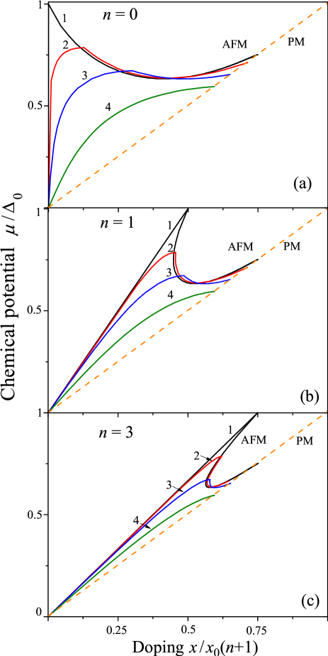
Figure 2: (Color online) Chemical potential $\mu$ versus doping $x$ for different values of $n$ [see Eq. (21)]: $n=0$ ($a$), $n=1$ ($b$), and $n=3$ (c). The different temperatures considered include: $T=0$ with solid (black) curves 1, $T/\Delta_{0}=0.1$ with solid (red) curve 2, $T/\Delta_{0}=0.2$ with solid (blue) curve 3, and $T/\Delta_{0}=0.35$ with solid (green) curve 4. Dashed (orange) lines correspond to $\mu(x)$ in the paramagnetic phase.

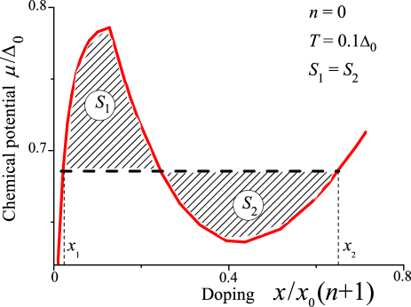
Figure 3: (Color online) Chemical potential $\mu$ versus doping $x$ for the homogeneous phase, $T/\Delta_{0}=0.1$ and $n=0$ [solid (red) line]. The horizontal dashed (black) line shows the Maxwell construction, with shaded areas $S_{1}=S_{2}$.

However, constructing Fig. 1 we assumed a priori that the ground state of the model is uniform. To check this assumption we plot the dependence of the chemical potential on the doping, for different temperatures. For different values of $n$ the results are shown in Figs. 2($a$, $b$, $c$). Curves $\mu(x)$ demonstrate three important features at temperatures lower than $T^{*}\approx 0.317\Delta_{0}$, for any $n$. First, the derivative $\partial\mu/\partial x$ is discontinuous at the transitions from commensurate to incommensurate AFM RiceMod , and from incommensurate AFM to the paramagnetic phase. The second major feature is that $\mu(x)$ has three different values for a range of doping $x$ at low $T$ if $n\gtrsim 1$, which means that we have to choose the lowest energy solution RiceMod . Thirdly, the derivative $\partial\mu/\partial x$ is negative at a finite range of doping.

This last peculiarity of $\partial\mu/\partial x$ eluded the attention of previous studies; yet, it has very important ramifications. Negative values of the derivative $\partial\mu/\partial x$ mean that the compressibility, $\kappa\propto\partial x/\partial\mu$, is negative. This negative compressibility indicates that the homogeneous state is unstable towards phase separation. In the phase-separated state the system segregates into two phases with different doping values. Let us denote these values as $x_{1}$ and $x_{2}$, and the volume fractions of the corresponding phases as $p_{1}$ and $p_{2}$, such that $p_{1}+p_{2}=1$. Then, the doping satisfies $x=p_{1}x_{1}+(1-p_{1})x_{2}$, and $p_{1}=(x_{2}-x)/(x_{2}-x_{1})$.

The values $x_{1}$ and $x_{2}$ can be found using the Maxwell construction (see, e.g., Ref. LeBellac, ). Figure 3 illustrates the latter concept: the horizontal dashed line is drawn in such a manner that the areas of the shaded regions, $S_{1}$ and $S_{2}$, are equal: $S_{1}=S_{2}$.

Using the Maxwell construction, the boundary $T_{PS}(x)$ between the homogeneous and phase-separated states is calculated. This boundary is shown by the dashed (red) curves in the $(x,T)$ phase diagrams drawn in Fig. 4, for different values of $n$.

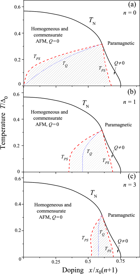
Figure 4: (Color online) Phase diagram of the Rice model RiceMod for $n=0$ ($a$), $n=1$ ($b$), and $n=3$ ($c$). The solid (black) curves represent the Néel temperature $T_{\textrm{N}}(x)$, which separates the paramagnetic and AFM phases. The dotted (blue) curves are $T_{Q}(x)$, the boundary between the commensurate ($Q=0$) and incommensurate ($Q\neq 0$) homogeneous AFM phases. The dashed (red) curve, $T_{PS}(x)$, is the boundary between the uniform and phase-separated (shaded areas) phases.

The phase with lower doping, $x_{1}$, is the commensurate AFM ($Q=0$) while the phase with higher doping, $x_{2}$, is the incommensurate AFM ($Q\neq 0$), as it can be readily seen from Figs. 2, 3. Thus, here the phase separation occurs due to the competition between two AFM states with different structures. So, it is natural that the boundary temperature $T_{Q}$ lies between two lines $T_{PS}$ separating the homogeneous and inhomogeneous states (see Fig. 4). The phase separation is absent for higher temperatures $T>T^{*}\approx 0.317\Delta_{0}$. This phase separation disappears simultaneously with the incommensurate AFM phase. The area of the incommensurate AFM phase in Fig. 4 decreases, when $n$ (which is proportional to the density of states in the non-magnetic band) increases. However, one must remember that in Figs. 2-4 the horizontal scale changes when $n$ changes.

IV Discussion

In the previous section we demonstrated that the incommensurate AFM state of the Rice model RiceMod is unstable toward phase separation. This feature is likely to have important consequences for the diverse set of materials where the nesting degradation may be responsible for the destruction of the magnetic phase: chromium and its alloys Review88 , pnictides and chalcogenides Fe_separation_experiment , doped AA-stacked graphene bilayer our_aa_phasep_preprint , and others. Here we would like to discuss the obtained results and compare these with other published works.

Above we used the mapping between the Rice model and the FFLO superconductor. However, usually, the phase separation is absent from the phase diagram of the FFLO superconductor. This has a very simple explanation: these diagrams are plotted as a function of the temperature and the Zeeman field (which is an analog of the chemical potential $\mu$ in the Rice’s model). The field, being an intensive thermodynamic quantity, does not allow for phase separation. Instead, the system experiences a first-order transition as a function of the Zeeman field ff . However, for cold atoms in an optical trap it may be possible to control not the field, but the polarization, which is an extensive quantity. In this case, phase separation occurs sheehy .

As we mentioned above, besides Eq. (6), it is possible to consider other types of spatially-inhomogeneous order parameters stripes_luo ; fflo_review . A particularly interesting possibility was discussed in Ref. gorkov_teit_prb2010, , where the known numerical results for the two-dimensional FFLO superconductor bukh_ann_phys1994 with an order parameter of the Larkin-Ovchinnikov’s type was applied to study the Rice model. It was proposed gorkov_teit_prb2010 that, upon small doping, the order parameter in real space forms domain walls. At a domain wall the gap vanishes locally, which makes these walls a preferred place for the accumulation of the doped charge. It was demonstrated bukh_ann_phys1994 ; gorkov_teit_prb2010 that the formation of these domain walls becomes energetically favorable for

$$\mu>\mu_{DW}\approx 0.655\Delta_{0}.$$ (22)

The value of $\mu_{DW}$ is somewhat smaller than

$$\mu^{2D}_{PS}\approx 0.7\Delta_{0},$$ (23)

which is the value of the chemical potential corresponding to the phase separation in the two-dimensional Rice model at $T=0$. Since at low doping the energy can be approximated by

$$E=E_{0}+\int_{0}^{x}\!\!\!\mu(x^{\prime})dx^{\prime}\approx E_{0}+\mu(0)x,$$ (24)

where $E_{0}$ is the energy of the undoped state, we must conclude that at low doping the phase-separated state is less favorable than the phase with domain walls. However, the difference

$$\mu_{PS}^{2D}-\mu_{DW}\approx 0.05\Delta_{0}$$ (25)

is small, and in real systems the balance may be shifted by the factors unaccounted by the present model (e.g., anisotropy, Coulomb interaction, disorder, etc.). Thus, the possibility of phase separation driven by the mechanism proposed in this paper should be kept in mind when experimental data are analyzed.

The experimental observation of phase separation in superconducting pnictides and chalcogenides, which may be approximately described by the Rice model RiceMod , was reported in several papers Fe_separation_experiment . For example, Park and co-authors Fe_separation_experiment found the coexistence of magnetic and non-magnetic domains with a typical size $\sim 65$  nm. This observation is in general agreement with our proposed mechanism. While our model predicts the separation into two magnetic phases, the AFM order in the incommensurate phase is weak, and the energy is close to the energy of the paramagnetic phase. Thus, either the AFM order parameter in the incommensurate phase is below experimental sensitivity, or, being affected by factors outside of our simple treatment, the weak phase itself is replaced by the paramagnetic state. The latter scenario is quite likely, given the small energy difference between the paramagnetic and incommensurate AFM states. If the incommensurate AFM is destroyed, phase separation occurs between the undoped commensurate AFM and the paramagnetic states. Such type of phase separation was discussed for AA-stacked graphene bilayers our_aa_phasep_preprint , whose band structure corresponds to the two-dimensional Rice model.

Let us briefly mention several complications not considered here, which, nonetheless, may be present in experimental systems, and influence the resulting phase diagram. In experiments, the electron and hole pockets may have non-identical non-spherical shapes and different Fermi velocities. How these factors affect the phase separation is a subject of further study. In the weak-coupling regime, Eq. (5), it is likely that sufficiently small deviations from the idealized model will not affect qualitatively the outcome of the calculations, provided that $V$ is not too weak.

Our calculations were performed in the weak-coupling limit. Would the phase separation survive outside of this regime? Note that in order to discuss the intermediate or strong-coupling regime, the Rice model is not a good starting point. Rather, a multi-orbital lattice Hamiltonian is a better approach. For such models the phase separation is a common phenomenon. dagotto_book ; other_pha_sep ; PSmultiHubbard Further, recent numerical studies of the Hubbard model at intermediate and strong coupling trembley_hubb reported phase separation at finite doping. Thus, it is likely that even for strong and intermediate interaction strengths it is possible to find a region of the model’s parameter space where phase separation occurs. Although, in such regimes the mechanism of phase separation cannot be described in terms of Fermi surface nesting.

To apply the theoretical results to experiments it is important to consider the effects of disorder. We know that the FFLO state is very fragile with respect to impurity scattering takada . Thus, our incommensurate AFM, which is the mathematical analog of the FFLO phase, is expected to be susceptible to microscopic imperfections. Therefore, we conclude that the disorder-induced modifications to the phase diagram is an open question which requires special attention.

The study of characteristic scales and geometry of the phase separated state is beyond the scope of this study since it requires additional information on the properties of the system, which are disregarded by the Rice model. For example, even in the simplest approach to this problem, the structure of the inhomogeneous state is governed by the interplay between long-range Coulomb interaction and the energy of the boundary between different phases. Coulomb Thus, it is reasonable to study the details of the phase-separated state only if the particular physical system is specified in detail.

In conclusion, we have demonstrated that the uniform ground state of the Rice model for an itinerant AFM with imperfect nesting is unstable with respect to electronic phase separation in a significant range of dopings and temperatures. In this range, the uniform system segregates into two AFM phases, one of which is the commensurate AFM, while the second is the incommensurate AFM. It is argued that such instability can occur in other models with imperfect nesting because this effect is driven by the competition between phases with different doping and different magnetic structures.

References

- (1)
- (2) T.M. Rice, Phys. Rev. B2, 3619 (1970).
- (3) E. Fawcett, Rev. Mod. Phys. 60, 209 (1988).
- (4) D.J. Singh, M.-H. Du, L. Zhang, A. Subedi, J. An, Physica C 469, 886 (2009).
- (5) A.B. Vorontsov, M.G. Vavilov, and A.V. Chubukov, Phys. Rev. B81, 174538 (2010).
- (6) L.P. Gor’kov, G.B. Teitel’baum, Phys. Rev. B 82, 020510(R) (2010).
- (7) P. Dai, J. Hu and E. Dagotto, Nature Physics 8, 709 (2012).
- (8) A.L. Rakhmanov, A.V. Rozhkov, A.O. Sboychakov, and Franco Nori, Phys. Rev. Lett. 109, 206801 (2012).
- (9) A.O. Sboychakov, A.L. Rakhmanov, A.V. Rozhkov, and Franco Nori, preprint arXiv:1302.1994 (unpublished).
- (10) L. P. Gor’kov and T. T. Mnatzakanov, Sov. Phys. JETP 36, 361 (1973).
- (11) J.T. Park et al., Phys. Rev. Lett. 102, 117006 (2009); D.S. Inosov et. al., Phys. Rev. B, 79, 224503 (2009); G. Lang, H.-J. Grafe, D. Paar, F. Hammerath, K. Manthey, G. Behr, J. Werner, and B. Büchner, Phys. Rev. Lett. 104, 097001 (2010); B. Shen, B. Zeng, G.F. Chen, J.B. He, D.M. Wang, H. Yang and H.H. Wen, EPL, 96, 37010 (2011).
- (12) P. Fulde and R.A. Ferrell, Phys. Rev. 135, A550 (1964).
- (13) A.I. Larkin, Yu.N. Ovchinnikov, Zh. Eksp. Teor. Fiz. 47, 1136 (1964) [Sov. Phys. JETP 20, 762 (1965)].
- (14) M. Le Bellac, F. Mortessagne, and G.G. Batrouni, Equilibrium and Non-Equilibrium Statistical Thermodynamics, (Cambridge Univ. Press, Cambridge 2004).
- (15) D.E. Sheehy and L. Radzihovsky, Annals of Physics, 322, 1790, (2007).
- (16) Q. Luo, D.-X. Yao, A. Moreo, and E. Dagotto, Phys. Rev. B 83, 174513 (2011).
- (17) Y. Matsuda and H. Shimahara, J. Phys. Soc. Jpn. 76, 051005 (2007); J.A. Bowers and K. Rajagopal, Phys. Rev. D66, 065002 (2002); C. Mora and R. Combescot, Phys. Rev. B 71, 214504 (2005);
- (18) H. Burkhardt and D. Rainer, Ann. Phys. 506, 181 (1994).
- (19) E. Dagotto, Nanoscale Phase Separation and Colossal Magnetoresistance: The Physics of Manganites and Related Compounds (Springer-Verlag, Berlin, 2003).
- (20) S. Yunoki, J. Hu, A. L. Malvezzi, A. Moreo, N. Furukawa, and E. Dagotto, Phys. Rev. Lett. 80, 845 (1998); A. Moreo, S. Yunoki, E. Dagotto, Science 283, 2034 (1999).
- (21) F. Bucci, C. Castellani, C. Di Castro, and M. Grilli, Phys. Rev. B52 6880 (1995); K.I. Kugel, A.L. Rakhmanov, A.O. Sboychakov, and D.I. Khomskii, ibid., 78, 155113 (2008); A.L. Rakhmanov, A.V. Rozhkov, A.O. Sboychakov, and F. Nori, Phys. Rev. B 85, 035408 (2012); A.O. Sboychakov, K.I. Kugel, and A.L. Rakhmanov, ibid., 76, 195113 (2007).
- (22) G. Sordi, K. Haule, and A.-M.S. Tremblay, Phys. Rev. B84, 075161 (2011).
- (23) S. Takada, Prog. Theor. Phys. 43, 27 (1970).
- (24) J. Lorenzana, C. Castellani, and C. Di Castro, Phys. Rev. B64, 235127 (2001); ibid., 64, 235128 (2001); R. Jamei, S. Kivelson, and B. Spivak, Phys. Rev. Lett. 94, 056805 (2005); K.I. Kugel, A.L. Rakhmanov, A.O. Sboychakov, N. Poccia, and A. Bianconi, Phys. Rev. B, 78, 165124 (2008); K.I. Kugel, A.L. Rakhmanov, A.O. Sboychakov, F.V. Kusmartsev, N. Poccia, and A. Bianconi, Supercond. Sci. Tech. 22, 014007 (2009).