Finsler geometrization of classic theory for fields

on the interphase boundary including monomolecular 2D-system

V. Balan, H.V. Grushevskaya, N.G. Krylova, A. Oana

Abstract.

We prove that the Ricci scalar curvature and the Berwald scalar curvature of a two-dimensional Finsler space, considered over a vector field on the 3-dimensional flat space, are naturally related to 2-dimensional electro-capillary phenomena effects observed for a compressed monolayer. The Cartan tensor and the nonlinear Barthel connection of the Finsler model are determined, and the geometric objects which depend on compression speed and on the characteristics of the electrically charged double layer are used in order to reveal several classes of structure formation within the phase transition of the first order.

MSC 2010: 53B40, 53C60.
Key-words: Finsler metric, Barthel connection, Ricci scalar curvature, Berwald scalar curvature, compressed monolayer, electrically charged double layer.

1 Introduction

The nano-structures, which are formed at the boundary which separates two distinct phases, may exhibit unique electro-physical and optical properties [1, 2, 3, 4]. A type of such structures is represented by the Langmuir-Blodgett (LB) monolayers, which are obtained by compressing a mono-molecular layer (monolayer) of amphiphilic molecules on the surface of a liquid subphase [5, 6, 7, 8], in case that the compression is accompanied by the first order phase transition [9, 10, 11, 12]. In [13, 14] a Finsler geometrization of the contribution of the electro-capillary interactions to an action $S$, which describes the motion of particles in the monolayer, was proposed. This (pseudo-)Finsler space has the specific feature that a part of the tangent vectors lie on the hypercone similar to light cones of Relativity Theory ([15, 16]). The Finsler structure relies on associated geometric vector bundles over the slit tangent space, which infers that the fundamental Finsler function (pseudonorm) may be considered as an action for physical systems. In particular, one has the 3-dimensional case where the Finsler function is associated to the physical system associated to a 2d-monolayer. In its essence, a bundle is a geometric structure whose associated projection mapping transforms a path which lies inside a fiber to a point (a set of null measure) of the base manifold. There exist similar examples in which a system within the physical space is given by means of a projection from a space with larger dimension than the base space of the physical system. This can be illustrated by the reducing of the hydrogen-like atom problem with its symmetry group $SO(4)$ to a consideration of the harmonic oscillator in the space with the symmetry group $SO(6)$. In such problems the projection of states from the 6-dimensional space to the physical (3,1)-dimensional space is constructed [17].

For the determined Finsler function of the monolayer we numerically produced a large number of indicatrix classes [14]. However, in the absence of the stability of such solutions, the link between these solutions and the real observed monolayer structures was not completely sustained. The principle of minimal action $S$ needs the fulfillment of the Euler-Lagrange equations for the Lagrange function $L$, which provides the action $\int L\,dt=S$. These are differential equations of second-order, hence the need to consider the specific structural (Jacobi) stability, which reveals the robustness/fragility of the second order system [18]. To this aim, one has to take into account that the obtained Finsler metric provides a specific class of invariant geometric objects of the Finsler bundle of tangent spaces, which naturally relate to the surface electrocapillary physical phenomena observed for the monolayer. We should note that the 2d-motion of particles within this in this monolayer is approximated by geodesics of the geometric structure.

The anomalous behavior of geometric objects like the Ricci and Berwald scalar curvatures $R_{c}$ and $B_{c}$, the Cartan tensor, and the nonlinear Barthel connection play a special role while developing the KCC theory of the model and constructing the associated invariants. We shall determine the relation between the anomalous behavior of these geometric objects and the behavior of compression isotherms $\tilde{\pi}-s$. For $LB$-structures, these isotherms exhibit a plateau, which is characteristic for the phase transition of the first order.

It is known [19, 20] that the necessary condition of phase state stability is a positiveness of Hessian in an expansion of energy increment over thermodynamic variables. By analogy one can study the stability of phase state by analyzing a Hessian for an expansion of Gibbs free energy [21]. With such an approach one can introduce a metric of a thermodynamic variables space to utilize Riemann geometry methods [22, 23]. The scalar curvature in such thermodynamic geometrization can be expressed in terms of such matter thermodynamics quantities as the compressibility $\kappa$, the thermal expansion, the heat capacity. It was expected that a priority of such approach would be the analysis of one geometric structure – the curvature, as generalized thermodynamic parameter, instead of a large number of thermodynamic inequalities. The heat capacity and compressibility have divergences at phase transitions. Divergences of the thermodynamic quantities should involve divergences of the curvature. However, for well-known Ruppeiner’s [24] and Weinhold’s [22, 23] metrics limited values of scalar curvatures in a critical point remain finite when trending one of above mentioned thermodynamic quantities to infinity at fixed other ones [25]. In [26] the thermodynamics was geometrized with a metric, scalar curvature of which diverges in a critical point. The Quevedo’s metric describes second-order phase transitions without metastable states satisfactorily [25]. A physical nature of the first order phase transition in a triple point is analogous to the second order phase transition [27]. But, in contrast to the second order phase transitions in the vicinity of the first order phase transition $\kappa$ and other thermodynamic quantities of matter change sign to opposite. In [25] it was proposed a metric of thermodynamic variables space, the scalar curvature of which both divergences and differs by sign for stable and metastable states in a critical point. But, unfortunately this metric is not invariant in respect to Legendre transformations. Thus, nowadays a problem of description of the first order phase transitions is still actual.

The goal of the present paper is to describe by means of the invariants of the 2D-Finsler space the acceleration of the molecules of the monolayer in the field of electro-capillary forces, whose contribution to the action is represented as a Finsler-type geometric structure associated to the interactions within the amphiphilic monolayer, and to study the structuring of the monolayer which undergoes phase transition.

2 The physical model

In [14], there is proposed a simple model of a monolayer of amphiphilic molecules. Hydrophilic parts of amphiphilic molecules are in an electrolyte and hydrophobic parts are outside. In water the hydrophilic parts of molecules dissociate on positively charged hydrogen ions and negatively charged hydrophilic groups (”heads”). The monolayer and the double electrically charged layer are regarded as a plane-parallel capacitor with the capacity $C$, and a charge $\pm Q$ on its plates. The potential difference ${\Phi}$ on the interphase boundary is determined by the formula

$$\Phi=\frac{Q}{C}=\frac{QD}{\varepsilon\varepsilon_{0}S}=\frac{q\rho(\vec{r},t)D}{\varepsilon\varepsilon_{0}},$$ (2.1)

where $q$ is the charge of one ionized molecule, $\rho(\vec{r},t)$ is the surface density of molecules in the monolayer, $\varepsilon_{0}$ is the dielectric constant, $\varepsilon$ is the dielectric permittivity, and $S$ is the area of the capacitor plates. The motion of ionized particles of the monolayer takes place in the potential of electro-capillary forces ([28, 29, 30, 31]). This is why - as shown in [14] - the particles possess, besides the kinetic energy and the energy of interparticle interactions $E_{c}$, a potential energy $U_{s}(r,t)$ due to the capillary interaction:

$$U_{s}(r,t)={\sigma}^{\prime}_{r}+\frac{{\sigma}^{\prime}_{t}}{\dot{r}}+\frac{\sigma}{r}$$ (2.2)

at an arbitrary point of the spherically-symmetric monolayer with the co-ordinates $(r,t)$, with $\rho$ having the explicit form:

$$\rho(r,t)=\rho_{0}e^{-\int{\frac{\dot{r}}{r}dt}}.$$ (2.3)

We shall further choose a cylindric orthogonal coordinate system ($r$, $\phi,\ z$), in which the spherically-symmetric monolayer is displaced in the plane $XY$ with $z=0$, and the center is located at the origin of coordinates; here the prime denotes the derivative with respect to the corresponding index, $\sigma$ is the surface tension of the monolayer (the energy of the 2d-membrane), determined by the following expression:

$$\sigma(r,t)=-\frac{\pi^{2}q^{2}}{\varepsilon\varepsilon_{0}}\rho_{0}^{2}\int{\dot{r}dt\,}r^{3}e^{-\int\limits_{t_{0}}^{t}{\frac{2\dot{r}}{r(t^{\prime})}\,dt^{\prime}}},$$ (2.4)

and $\rho_{0}$ is the monolayer density at the initial moment $t_{0}$.

3 The Lagrange and Finsler structures associated to the model

One can neglect the particle interaction energy $E_{c}$, since the negatively charged ”heads” are surrounded by the positively-charged ”coats” of ions and water molecules. Then, for the general case of a particle which moves in the potential $U_{s}(r,t)$ (2.2) in a plane, it is possible to write down the Lagrange function $L$ corresponding to this motion, in the form:

$$L=m\frac{dr^{2}+r^{2}d\varphi^{2}}{2dt^{2}}-U_{s}(r,t),$$ (3.1)

where the first term in the expression (3.1) is a kinetic energy. The non-relativistic metric function $dF$ of the monolayer in the Euclidean 3d-space reads [14]:

$$dF=mc^{2}dt-L_{0}(x,y)dt+eAdz/c,$$ (3.2)

where $L_{0}$ is the Lagrange function which is considered without taking into account effects of electro-capillarity, $dz\sim\dot{r}dr/D$, $z$ is the projection of the position vector $\vec{R}$ of a particle onto the $Z$-axis, $c$ is the speed of light, and we have:

$${e\over c}Adz=-{q\over D}\dot{r}dr\int|E^{\prime}|dt$$ (3.3)

due to the relation

$${1\over c}{\partial\over\partial t}\vec{\nabla}\times\vec{A}=-\vec{\nabla}\times\vec{E}^{\prime},$$ (3.4)

where $\vec{E}^{\prime}\ =\vec{\nabla}\Phi\$. Since the monolayer exhibits non-vanishing curvature, the particle will have an accelerated motion with the acceleration value $a_{u}$: $\dot{r}\sim a_{u}t$. This means that the ranges of variation for the variable $z$ differ for various directions $(dx,dy)$. Taking into account that $dz\sim a_{u}t\,dr/D$, the space of particle motion is a space of linear elements $(x,y,z,t={D\over a_{u}}{\partial z\over\partial r})$ with the underlying geometry of Finsler type, as stated in the Introduction, and we have

$$dF\sim{e}\ dz={q\ a_{u}t\over D}dr.$$ (3.5)

The equation of the figuratrix $H$ can be obtained from the following expression [16, pp.34,43-44], [32]:

$$\frac{\partial g_{ik}(x,\dot{x})}{\partial x^{h}}\dot{x}^{i}\dot{x}^{k}=-\frac{\partial g^{ik}(x,p)}{\partial x^{h}}p_{i}p_{k},\ \dot{x}^{i}=g^{ij}p_{j},\;p_{i}=g_{ij}\dot{x}^{j},$$ (3.6)

if we take into account that

$$F^{2}(x,\dot{x})=g_{ik}(x,\dot{x})\dot{x}^{i}\dot{x}^{k},\ H^{2}(x,p)=g^{ik}(x,p)p_{i}p_{k}.$$ (3.7)

From this, it follows that the metric function $F$ is connected with the Hamiltonian $H$ by the following relation:

$$\frac{\partial F^{2}(x,\dot{x})}{\partial x^{h}}=-\frac{\partial H^{2}(x,p)}{\partial x^{h}}.$$ (3.8)

Now, we differentiate the right hand side of (3.8), and take into consideration the dependence of the kinetic energy on momentum only. Then, eq. (3.8) gets the form

$$\frac{\partial F^{2}(x,\dot{x})}{\partial x^{h}}=-2H\frac{\partial U_{s}(x,\dot{x})}{\partial x^{h}}.$$ (3.9)

For potential energy $U_{s}$ in the expression (3.9) we shall use the model potential (2.2)–(2.4). Then, substituting the expressions (2.2)–(2.4) into (3.9), we rewrite the last relation as

$$\begin{array}[]{ll}\frac{\partial F^{2}(x,\dot{x})}{\partial x^{h}}&=-2E_{\kappa}\frac{\partial}{\partial x^{h}}\frac{\pi^{2}q^{2}}{\varepsilon\varepsilon_{0}}\rho_{0}^{2}\int\dot{r}\,dt\,\left(-2e^{-\int\limits_{t_{0}}^{t}\frac{2}{r}\dot{r}\,dt^{\prime}}(3-2\frac{r\partial}{\dot{r}\partial t}\int\limits_{t_{0}}^{t}\dot{r}\,dt^{\prime}/r)-e^{-\int\limits_{t_{0}}^{t}\frac{2}{r}\dot{r}\,dt^{\prime}}\right)r^{2}\\ &=-2E_{\kappa}\frac{\partial}{\partial x^{h}}\frac{\pi^{2}q^{2}}{\varepsilon\varepsilon_{0}}\rho_{0}^{2}\left(-3\int{\dot{r}\,dt}e^{-\int\limits_{t_{0}}^{t}\frac{2}{r}\dot{r}dt^{\prime}}r^{2}\right),\end{array}$$ (3.10)

where $E_{\kappa}$ is an arbitrarily fixed value of the Hamiltonian function ${H}$.

4 From metric to field equation

We shall further examine the state of the monolayer at the beginning of the compression $t\to t_{0}=0$, when the monolayer represents itself a two-dimensional gas. This is the case of such concentrations $\rho(r,t)$, $\rho\to\rho_{0}$, at which the interaction of the particles of the monolayer may be neglected. In this case velocities of particles are very small: $\dot{r}=\delta\to 0$ and $r=r(0)+\dot{r}t$, as $t\to 0$. Then, taking into account the condition $\dot{r}=-a_{u}t$, $a_{u}>0$, the dependence $\rho(r,t)$ gets the following explicit form:

$$\begin{array}[]{ll}\rho(r,\dot{r}\to 0)&=\left.\rho_{0}e^{-\int_{0}^{t}{\dot{r}\over r}dt^{\prime}}\right|_{\dot{r}=\delta}\to\left.\rho_{0}e^{-\int_{0}^{t}{\dot{r}dt^{\prime}\over r(0)+\dot{r}t^{\prime}}}\right|_{\dot{r}=-a_{u}t}=\vskip 6.0pt plus 2.0pt minus 2.0pt\\ &=\rho_{0}e^{-\int_{0}^{t}{-a_{u}{t^{\prime}}dt^{\prime}\over r(0)-a_{u}{t^{\prime}}^{2}}}=\rho_{0}e^{-{1/2}\int_{0}^{t}{d(r(0)-a_{u}{t^{\prime}}^{2})\over r(0)-a_{u}{t^{\prime}}^{2}}}=\left.\rho_{0}\left({r(0)\over r(0)-|\dot{r}|t}\right)^{1/2}\right|_{\dot{r}\to 0},\end{array}$$ (4.1)

where $r(0)=r(t=0)$. For small compression time $t\to 0$, by taking into account (4.1), the quadratic metric (3.10) without the kinetic energy part can be transformed to the following form:

$$\begin{array}[]{ll}F^{2}&\sim\;\;-2E_{\kappa}\frac{\pi^{2}q^{2}}{\varepsilon\varepsilon_{0}}\rho_{0}^{2}\left(3\int{a_{u}t\,dt}e^{-\int\limits_{t_{0}}^{t}\frac{2}{r}\dot{r}dt^{\prime}}r^{2}\right)=-6E_{\kappa}\frac{\pi^{2}q^{2}}{\varepsilon\varepsilon_{0}}a_{u}\int t\,dt\,\rho^{2}(r,t)\,r^{2}\vskip 6.0pt plus 2.0pt minus 2.0pt\\ &=-6E_{\kappa}\frac{\pi^{2}q^{2}}{\varepsilon\varepsilon_{0}}a_{u}\rho_{0}^{2}\,r(0)\int(r(0)t-a_{u}t^{3})\,dt=-3E_{\kappa}\frac{\pi^{2}q^{2}}{\varepsilon\varepsilon_{0}}a_{u}\rho^{2}(r,t)\,t^{2}\,(r^{2}-{1\over 2}a_{u}rt^{2})\vskip 6.0pt plus 2.0pt minus 2.0pt\\ &=-3E_{\kappa}\frac{\pi^{2}q^{2}}{\varepsilon\varepsilon_{0}}a_{u}\rho^{2}(r,t)\,t^{2}\,[r^{2}+{\cal{O}}(t^{2})].\end{array}$$ (4.2)

Due to the admissible freedom in choosing the fixed value of the Hamiltonian function $H$, one can assume that

$$E_{\kappa}=-1\mbox{ for }\int|E^{\prime}|dt=\sqrt{3}\pi.$$ (4.3)

The assumption (4.3) allows us to rewrite the part (4.2) of the quadratic metric and the metric function (3.5) without the kinetic energy part as

$$\left.F^{2}(x,\dot{x})\right|_{t\to 0}\equiv F^{2}(x,\dot{x},\dot{t})\sim\frac{3\pi^{2}q^{2}}{\varepsilon\varepsilon_{0}}a_{u}\rho^{2}(r,t)\,{t}^{2}\,{r}^{2},$$ (4.4)

$$F(x,\dot{x},\dot{t})\sim-\sqrt{3}\pi{q\ a_{u}\over D}{t}{r}$$ (4.5)

Comparing (4.4) with (4.5), we get the acceleration $a_{u}$ in its explicit form

$$\begin{split}{q\sqrt{a_{u}}\over\sqrt{\varepsilon\varepsilon_{0}}}\sim\frac{q\rho(r,t)\,D}{\varepsilon\varepsilon_{0}}.\end{split}$$ (4.6)

The comparison of (4.6) and (2.1) leads to the approximation

$$\begin{split}a_{u}\sim{\varepsilon\varepsilon_{0}\over q^{2}}\left(\frac{q\rho(r,t)\,D}{\varepsilon\varepsilon_{0}}\right)^{2}={\varepsilon\varepsilon_{0}\over q^{2}}\left(\Phi\right)^{2}.\end{split}$$ (4.7)

Now, one can consider the kinetic energy part of the action (3.2). It is easy to see that $m\vec{\dot{r}}$ is a flux density per one particle which is proportional to a flux density $\int\rho\vec{\dot{r}}\,d^{2}r$ normalized to the area $S_{1}=\pi r^{2}(0)~{}$:

$$m\dot{r}\sim\int{\rho\dot{r}\over\pi r^{2}(0)}\,d^{2}r.$$ (4.8)

Substituting (3.5, 4.3, 4.7) into (3.2), rewriting the kinetic energy term in consideration of (4.8), and integrating, one gets the action $F$ in the form

$$F=\int dF=\int mc^{2}dt-\int\int{\alpha\over\rho_{0}}{{\dot{r}}^{2}\over 2\pi r(0)^{2}}\rho^{2}\,dtd^{2}r-{q\over D}\int t{\varepsilon\varepsilon_{0}\over q^{2}}\left(\Phi\right)^{2}d^{2}r,$$ (4.9)

with accuracy up to coefficient $\alpha$. We consider the coefficient given by the following relation:

$$\alpha={|q|D\over 2\varepsilon\varepsilon_{0}}$$ (4.10)

and choose the initial value $\rho_{0}$ as

$$\begin{split}\rho(0)\propto{1\over q^{2}}.\end{split}$$ (4.11)

Assuming that $q=-|q|$ and due to $t=\int dt$, after substituting the expressions (4.10) and (4.11) into the (4.9), one gets that

$$\int dF=\int mc^{2}dt-{|q|\varepsilon\varepsilon_{0}\over D}\left[\int\int\left({qD\over\varepsilon\varepsilon_{0}}\right)^{2}\,{{\dot{r}}^{2}\over 4\pi r^{2}(0)}\rho^{2}\,dt\,d^{2}r-\int dt\,\int d^{2}r{1\over q^{2}}\left(\Phi\right)^{2}\right].$$ (4.12)

Due to the (4.1), the term $\rho^{2}\dot{r}^{2}/(4\,r^{2}(0))$ which enters into the second term of (4.12) can be replaced by $\left({\partial\rho(r,t)\over\partial t}\right)^{2}$, since:

$$\begin{array}[]{ll}\left({\partial\rho(r,t)\over\partial t}\right)^{2}&={1\over 4}\dot{r}^{2}\rho_{0}^{2}{r(0)\over(r(0)-|\dot{r}|\,t)^{3}}={\rho^{2}\dot{r}^{2}\over 4r^{2}(0)(1-|\dot{r}|t/r(0))^{2}}\vskip 6.0pt plus 2.0pt minus 2.0pt\\ &\approx{\dot{r}^{2}\rho^{2}\over 4r^{2}(0)(1-2|\dot{r}|t/r(0))}\to{\dot{r}^{2}\rho^{2}\over 4r^{2}(0)},\qquad\mbox{ as }t\to 0.\end{array}$$ (4.13)

By substituting (4.13) into (4.12) and by taking into account the expression (2.1), one obtains that

$$\begin{array}[]{ll}\int dF&=\int mc^{2}dt-{|q|\varepsilon\varepsilon_{0}\over D}\left[\int dt{1\over\pi}\int d^{2}r\left({\partial\over\partial t}{q\rho(r,t)D\over\varepsilon\varepsilon_{0}}\right)^{2}-\int dt\int d^{2}r{1\over q^{2}}\left(\Phi\right)^{2}\right]\vskip 6.0pt plus 2.0pt minus 2.0pt\\ &=\int mc^{2}dt-{|q|\varepsilon\varepsilon_{0}\over D}\left[\int dt{1\over\pi}\int d^{2}r\left({\partial\over\partial t}\Phi\right)^{2}-\int dt\int d^{2}r{1\over q^{2}}\left(\Phi\right)^{2}\right].\end{array}$$ (4.14)

The quantity $\Pi^{\prime}$, which is conjugated to ${\partial\over\partial t}\Phi$ and equal to

$$\begin{split}\Pi^{\prime}={2\over\pi}{\partial\over\partial t}\Phi,\end{split}$$ (4.15)

is called the momentum of the field $\Phi$. We shall establish the physical meaning of (4.14). To this aim, it is necessary to add and subtract the gradient of the field $\Phi$, which is multiplied with $\varepsilon\varepsilon_{0}$:

$$\begin{split}{|q|\varepsilon\varepsilon_{0}\over D}\left({\Phi\over D}\right)^{2}\sim{|q|\varepsilon\varepsilon_{0}\over D}\left(\vec{\nabla}\Phi\right)^{2}.\end{split}$$ (4.16)

By substituting (4.15) and (4.16) into (4.14), one obtains that

$$\begin{split}dF=mc^{2}dt-dt{|q|\varepsilon\varepsilon_{0}\over D}\int d^{2}r\left\{{1\over 2}\Pi^{\prime}{\partial\over\partial t}\Phi-\left(\vec{\nabla}\Phi\right)^{2}-{1\over q^{2}}\left(\Phi\right)^{2}\right\}-{|q|\varepsilon\varepsilon_{0}\over D}dt\int d^{2}r\left({\Phi\over D}\right)^{2}.\end{split}$$ (4.17)

According to field theory [33, 34], the term in braces which enters into (4.17) is the Lagrangian density $\mathcal{L}$ of the field $\Phi$ stipulated by electrocapillary interactions:

$$\begin{split}\mathcal{L}={1\over 2}\Pi^{\prime}{\partial\over\partial t}\Phi-\left(\vec{\nabla}\Phi\right)^{2}-{1\over q^{2}}\left(\Phi\right)^{2}.\end{split}$$ (4.18)

This infers that the quantity ${1\over q^{2}}$ is a squared mass of the electrocapillary field $\Phi$.

We shall choose the initial value $r(0)$, such that this satisfies the law of conservation of matter. Under these circumstances, the duration $T={R_{0}\over|V|}$ for which the initial radius $R_{0}$ compresses up to zero (a point), is approximatively equal to the time consumed by the particle which moves with the speed $\dot{r}$, travelling along a distance which does not exceed $|V|T$, to the barrier, and further, jointly with the barrier, along a distance less than $|V|T$ to the center of the monolayer:

$$\begin{split}{R_{0}\over|V|}<{2|V|T\over|\dot{r}|},\end{split}$$ (4.19)

where $V$ is the compression speed. The condition (4.19) for the arbitrary point $r(0)$ of the monolayer can be expressed as

$$\begin{split}{r(0)\over|V|}<{2|V|t\over|\dot{r}|}.\end{split}$$ (4.20)

The velocity limitation (4.20) allows us to choose $r(0)$ as

$$\begin{split}{r(0)\over|V|t}\leq{2|V|\over|\dot{r}|}.\end{split}$$ (4.21)

For the initial conditions (4.11) and (4.21), the kinetic energy term entering into (4.14) can be rewritten in the following form:

$$\begin{array}[]{l}{|q|\varepsilon\varepsilon_{0}\over D}\left[\left({qD\over\varepsilon\varepsilon_{0}}\right)^{2}\,\int{{\dot{r}}^{2}\over 4\pi r^{2}(0)(1-2|\dot{r}|t/r(0))}\rho^{2}\,d^{2}r\right]={|q|\varepsilon\varepsilon_{0}}\left[\left({q\over\varepsilon\varepsilon_{0}}\right)^{2}\,\int{\rho\over 4\pi r^{2}(0)}\rho_{0}{{\dot{r}}^{2}\over 1-{\dot{r}^{2}\over V^{2}}}\,D\,d^{2}r\right]\vskip 6.0pt plus 2.0pt minus 2.0pt\\ \qquad={\varepsilon\varepsilon_{0}\over|q|}\left[\left({q\over\varepsilon\varepsilon_{0}}\right)^{2}\,\int{\rho\over 2\pi r^{2}(0)}{{\dot{r}}^{2}\over 1-{\dot{r}^{2}\over V^{2}}}\,d^{3}R\right]={2\varepsilon\varepsilon_{0}\over|q|\,D}\left[\left({q\,D\over 2\varepsilon\varepsilon_{0}}\right)^{2}\,\int{\rho_{V}\over\pi r^{2}(0)\,D}{{\dot{r}}^{2}\over 1-{\dot{r}^{2}\over V^{2}}}\,d^{3}R\right]\vskip 6.0pt plus 2.0pt minus 2.0pt\\ \qquad=\int{P^{2}\over 2Z_{\kappa}}\,{\rho_{V}\over\pi r^{2}(0)\,(D/2)}\,d^{3}R,\end{array}$$ (4.22)

where

$$Z_{\kappa}={|q|D\over 2\varepsilon\varepsilon_{0}},\vskip 6.0pt plus 2.0pt minus 2.0pt$$ (4.23)

$${P^{2}}=Z^{2}_{\kappa}{{\dot{r}}^{2}\over 1-{\dot{r}^{2}\over V^{2}}},\vskip 6.0pt plus 2.0pt minus 2.0pt$$ (4.24)

$$\rho_{V}=\left\{\begin{array}[]{lr}\rho&\mbox{if}\ z=0,\\ 0&\mbox{if}\ z\neq 0.\end{array}\right.$$ (4.27)

It follows then that the occurrence of $Z_{\kappa}$ is related with the existence of the additional third dimension, i.e., this is a mass of the particle which freely moves in the 3d-space and has the squared momentum $P^{2}$ defined by the expression similar to a relativistic one in the plane of the monolayer. The number density describing a particle distribution in this 3d-space is $\rho_{V}$. The squared three-dimension-mass $Z_{\kappa}^{2}$ determines the quadratic charge $q^{2}$, as follows:

$$2(Z_{\kappa}^{2}/\beta)=q^{2},\qquad\beta={D^{2}\over 2\varepsilon^{2}\varepsilon^{2}_{0}}.$$ (4.28)

In principle, we may double the dimension of the space from 3 to 6, by means of complexifying the variables, and expecting, by analogy, identical relations between the mass of the particle and the mass of the field, which is related to the exceeding complex coordinate. This analogy has already been considered in [17], if this 6-dimensional manifold is regarded as a 2-dimensional spinor space with two time-like coordinates. In [17], the free motion of a particle with mass $Z$ takes place in a 6-dimensional manifold with two space-like complex coordinates (a flat 2-dimensional spinor space) and two time-like coordinates. The projection of the movement of such a particle with the symmetry group $SO(6)$-equations [17, equations (22) and (61)] - on the 4-dimensional space-time (3,1) is described by the wave equation of the hydrogen-like atom with the symmetry group $SO(4)$-equation [17, equation (49)] – at the non-relativistic limit. Here the square of the charge $e$ and mass $m_{e}$ of the electron are proportional to the square of the mass $Z$ [17]:

$$2Z^{2}=e^{2}.$$ (4.29)

Comparing (4.28) with (4.29), we conclude that the projection of the motion of the free particle from the spinor 2-dimensional complex space and 2-dimensional time onto the space-time (3,1) is at the non-relativistic limit a complex analogue of the motion in the 3-dimensional space endowed with Finsler metric.

At the end we remark a peculiarity of the obtained action (4.17), namely the fact that it contains a re-normalized field mass $m_{f}$ due to the adding the term in (4.16):

$$\begin{split}dF=mc^{2}dt-dt{|q|\varepsilon\varepsilon_{0}\over D}\int d^{2}r\left\{{1\over 2}\Pi^{\prime}{\partial\over\partial t}\Phi-\left(\vec{\nabla}\Phi\right)^{2}-m_{f}^{2}\left(\Phi\right)^{2}\right\}\end{split}$$ (4.30)

where

$$m_{f}^{2}={1\over q^{2}}-{1\over D^{2}}.$$ (4.31)

In this way, at the limit of small concentrations, the energy of molecules in the compressed Langmuir monolayer on the subphase surface is determined by the rest mass of the particles and the electro-capillary field contribution to action owing an inner ”spinor”  degree of freedom. The physical meaning of this contribution is the jump of the surface tension of the interphase boundary between liquid and air, while dropping amphiphilic molecules on the surface of the subphase under the conditions of the moving barrier.

Thus, the fundamental function $F$ of our problem is not defined on the whole tangent space, but only on certain distributions over $\widetilde{TM}$ – the slit tangent space. In the general case, one considers the vertical sub-bundle $VTM=Ker(d\pi)$ of the vector bundle $(TTM,d\pi,TM)$ provided by the kernel of the linear mapping $d\pi$, and the supplementary sub-bundle $HTM=Ker(N)$ is provided by a Barthel connection $N:TTM\to VTM,\ N=(N^{j}_{i}(x,y))_{i,j\in\overline{1,n}}$, which satisfies $N\circ i=\left.id\right|_{VTM}$ (where $i:VTM\to TTM$ is the canonic inclusion). This leads to the Whitney decomposition [35, 36]

$$TTM=HTM\oplus VTM,$$ (4.32)

and induces a local adapted bases for the appropriate sections of these sub-bundles,

$$\left\{\delta_{i}={\delta\over\delta x_{i}}={\partial\over\partial x_{i}}+N^{j}_{i}{\partial\over\partial y_{j}}\right\}\subset\Gamma(HTM),\quad\left\{\dot{\partial}_{i}={\partial\over\partial y_{i}}=\right\}\subset\Gamma(VTM).$$ (4.33)

The related dual splitting $T^{*}TM=H^{*}TM\oplus V^{*}TM$ leads to similar dual bases,

$$\left\{dx_{i}\right\}\subset\Gamma(H^{*}TM),\quad\left\{\delta y_{i}=dy_{i}+N^{i}_{j}dx_{j}\right\}\subset\Gamma(V^{*}TM).$$ (4.34)

In the following section we shall consider the generalized Finsler structure, whose fundamental function $F$ is a metric function of the monolayer compressed by the barrier, considered at different speeds $V$.

5 Monolayer structuring process in terms of Finsler space invariants

In this section we analyze the geometric invariants of the particle motion within the monolayer, which is compressed by the barrier and provide physical interpretations of the corresponding specific behavior.

The electro-capillary potential energy $U_{s}(r,t)$ of the particle at a point $r(t)$ of the mono-molecular layer has the following explicit form [14]:

$$\begin{array}[]{ll}U_{s}(r,t)=&-\frac{\pi^{2}q^{2}}{\varepsilon\varepsilon_{0}}\frac{\rho_{0}^{2}}{R_{0}^{2}}\left({\left({-\frac{4}{3}r^{5}+\frac{16}{15}(|V|t)r^{4}+\frac{1}{30}(|V|t)^{2}r^{3}}\right.}\right.\vskip 6.0pt plus 2.0pt minus 2.0pt\\ &+\left.{\frac{1}{45}(|V|t)^{3}r^{2}+\frac{1}{45}(|V|t)^{4}r+\frac{2}{45}(|V|t)^{5}-r^{5}\frac{|V|}{\dot{r}}}\right)\left.{e^{\frac{2|V|t}{r}}-\frac{4}{45}\frac{(|V|t)^{6}}{r}\mbox{Ei}\left[{\frac{2|V|t}{r}}\right]}\right),\end{array}$$ (5.1)

where $\mbox{Ei}\left[{\frac{2|V|t}{r}}\right]$ is the exponential integral and $m$ is the molecular mass. The non-relativistic action $dl$ is defined by the relation

$$dl=mc^{2}dt-Ldt.$$ (5.2)

The substitution of the expressions (3.1) and (5.1) into (5.2) gives

$$\begin{array}[]{ll}dl=&mc^{2}\dot{\xi}-m\frac{\dot{r}^{2}+r^{2}\dot{\varphi}^{2}}{2\dot{\xi}}-\frac{\pi^{2}q^{2}}{\varepsilon\varepsilon_{0}}\frac{\rho_{0}^{2}}{R_{0}^{2}}\left({\left({-\frac{4}{3}r^{5}+\frac{16}{15}(|V|t)r^{4}+\frac{1}{30}(|V|t)^{2}r^{3}}\right.}\right.\vskip 6.0pt plus 2.0pt minus 2.0pt\\ &+\left.{\frac{1}{45}(|V|t)^{3}r^{2}+\frac{1}{45}(|V|t)^{4}r+\frac{2}{45}(|V|t)^{5}-r^{5}\frac{|V|}{\dot{r}}\dot{\xi}}\right)\left.{e^{\frac{2|V|t}{r}}-\frac{4}{45}\frac{(|V|t)^{6}}{r}\mbox{Ei}\left[{\frac{2|V|t}{r}}\right]}\right)\dot{\xi},\end{array}$$ (5.3)

where $\dot{\xi}$, $\dot{r}$, and $\dot{\varphi}$ correspond to the derivatives of $t$, $r$, and $\phi$ with respect to the evolution parameter $\tau$, respectively. We rewrite this action $dl$ as

$$dl=A{\dot{\xi}^{2}\over\dot{r}}+B\dot{\xi}-C\frac{(\dot{r}^{2}+r^{2}\dot{\phi}^{2})}{2c^{2}\dot{\xi}},$$ (5.4)

where the parameters $A,\ B,\ C$ are given by

$$\begin{array}[]{l}A=p\left|V\right|r^{5}e^{\frac{2\left|V\right|t}{r}},\vskip 6.0pt plus 2.0pt minus 2.0pt\\ B=mc^{2}-p\left({\left({-\frac{4}{3}r^{5}+\frac{16}{15}(|V|t)r^{4}+\frac{1}{30}(|V|t)^{2}r^{3}+\frac{1}{45}(|V|t)^{3}r^{2}+\frac{1}{45}(|V|t)^{4}r}\right.}\right.\vskip 6.0pt plus 2.0pt minus 2.0pt\\ \qquad\quad\left.{+\frac{2}{45}(|V|t)^{5}}\right)\left.{e^{\frac{2|V|t}{r}}-\frac{4}{45}\frac{(|V|t)^{6}}{r}\mbox{Ei}\left[{\frac{2|V|t}{r}}\right]}\right),\vskip 6.0pt plus 2.0pt minus 2.0pt\\ C=mc^{2},\quad\mbox{ where }p=\frac{\pi^{2}q^{2}}{\varepsilon\varepsilon_{0}}\frac{\rho_{0}^{2}}{R_{0}^{2}},\ \dot{r}=\frac{x\dot{x}+y\dot{y}}{r}.\end{array}$$ (5.5)

The length element $F$ (which provides a Berwald-Mòor type metric, [37, 38]) can be defined by means of the volume element $d\widetilde{V}$, which depends on the differentials of the Cartesian coordinates. Due to the stated above relation $\dot{r}\sim a_{u}t$, it follows that the 4d-volume $V_{4}$ is equal to $d\vec{l}\wedge\vec{\dot{\xi}}\sim(\vec{\dot{r}}\wedge\vec{\dot{\xi}}\,)^{2}$ at $dt=\vec{\dot{\xi}}$, and the equation (4.4) for the square $F^{2}$ of the metric function $F\sim dl$ can be written as:

$$\begin{split}F^{2}\sim(\dot{t}\dot{r})^{2}\sim|(\vec{\dot{\xi}}\cdot d\vec{r})|^{2}\sim\dot{\xi}|d\vec{l}|=\dot{\xi}\,dl.\end{split}$$ (5.6)

Hence, (5.4) determines a quadratic metric $F^{2}\sim dl{\dot{\xi}}$ (5.6) of the following form:

$$F^{2}=A{\dot{\xi}^{3}\over\dot{r}}+B\dot{\xi}^{2}-C\frac{(\dot{r}^{2}+r^{2}\dot{\phi}^{2})}{2c^{2}},$$ (5.7)

where the parameters $A,\ B,\ C$ are given by the system (5.5). Renormalizing the relation (5.7) by using

$$\dot{\tilde{r}}=\frac{\dot{r}}{c},\quad\dot{\tilde{x}}=\frac{\dot{x}}{c},\quad\dot{\tilde{y}}=\frac{\dot{y}}{c}.$$ (5.8)

we express the equation of the metric $F$ in terms of these normalized coordinates:

$$F^{2}=\tilde{A}{{\dot{\xi}}^{3}\over\dot{\tilde{r}}}+B{\dot{\xi}}^{2}-C\frac{({\dot{\tilde{r}}}^{2}+r^{2}{\dot{\tilde{\phi}}}^{2})}{2},\quad\tilde{A}={A\over c}.$$ (5.9)

For simplifying the notations, we shall further omit in our considerations the symbol ”$\sim$”.

A)

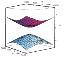
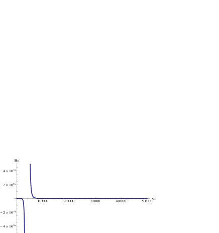
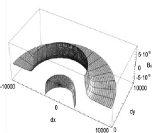
B)

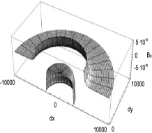
C)

D)

E)

F)

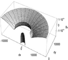
Figure 1: Indicatrices (from the left) which relate to the Berwald curvature $B_{C}$ (2d- and 3d-images in the middle and right respectively) having a single peculiarity for $x_{0}=$0.0796186, 0.079618558, 0.079618557, 0.0796185568, 0.0796185566,  0.07961855657, 0.0796185565, for $B=0.922721$ (A), 0.0315175 (B), 0.0102984 (C), 0.00605459 (D), 0.00181076 (E), 0.00117419 (F) respectively. Here $C=423\times 10^{-10}$, $A=4.78079\times 10^{7}$, $V=15.0$.

A)

B)

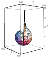
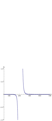
C)

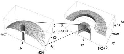
D)

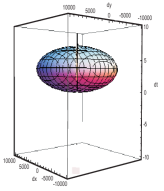
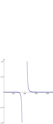
E)

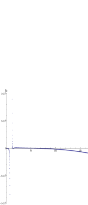
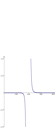
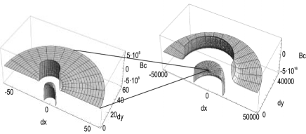
Figure 2: Indicatrices (from the left) which relate to the Berwald curvature $B_{C}$ (2d- and 3d-images in the middle and right respectively) having two peculiarities for $x_{0}=$ 0.0796185564, 0.0796185562, 0.079618556, 0.079618555, 0.079618553, 0.0796185 for $B=-0.00243306$ (A), $-0.0109207$ (B), $-0.0321398$ (C), $-0.0745781$ (D), $-1.19919$ (E) respectively. Here $C=423\times 10^{-10}$, $A=4.78079\times 10^{7}$, $V=15.0$.

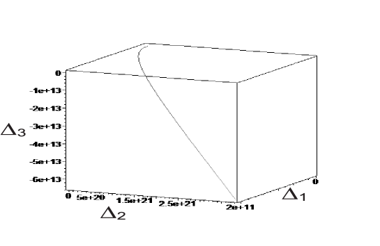
Figure 3: The 3d curve related to signature.

(a)                                                      (b)

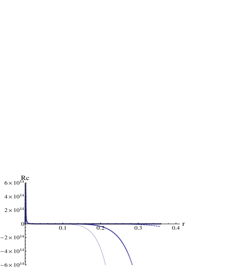
Figure 4: The dependence of $R_{C}$ on the reference radius $r$ at different monolayer compressing speeds (a) $V=10^{-15}$ (thick solid line), $10^{-10}$ (dashed line), $10^{-8}$ (dotted line), $10^{-7}$ m/sec (thin solid line); (b) $10$ m/sec for $t=0.01,\ \dot{\xi}=0.00001,\ \dot{r}=0.01,\ \dot{\phi}=0$.

Figure 5: The dependence of the curvature radius $1/R_{C}$ on $V$.

Using the following experimental values for the parameters

$$m=47\times 10^{-26}\mbox{kg},\ p=8.93434\times 10^{9}\mbox{ joule/m}^{5},\ c=3\times 10^{8}\mbox{m/sec},$$ (5.10)

we shall perform an illustrative simulation. When the speed $V$ of the monolayer compression tends to zero, the coefficient $A$ tends to zero as well, and the indicatrix is a hyperboloid of two sheets – which is characteristic for the Minkowski space. But at high speeds ($V$), there exists a region of Space–Time, in which the structural topological form of the indicatrix dramatically changes as Figs. 1 and 2 clearly show. We shall further analyze several invariants of the Finsler space endowed with the metric function $F$ given by (5.9).

Using the following steps, one can determine the horizontal $hh$-component $R^{i}_{jkl}$ of the curvature Ricci tensor $\Omega^{i}_{jkl}$:

$$g_{ij}={1\over 2}{\partial^{2}F^{2}\over\partial y^{i}\partial y^{j}},$$ (5.11)

$$G^{i}(y)={1\over 4}g^{il}(y)\left\{{\partial^{2}F^{2}(x,y)\over\partial x^{k}\partial y^{l}}y^{k}-{\partial F^{2}(x,y)\over\partial x^{l}}\right\}={1\over 4}g^{il}(y)\left\{2{\partial g_{jl}\over\partial x^{k}}(y)-{\partial g_{jk}\over\partial x^{l}}(y)\right\}y^{j}y^{k},$$ (5.12)

$$N^{i}_{j}(y)={\partial G^{i}\over\partial y^{j}}(y),$$ (5.13)

$${\delta\over\delta x^{s}}={\partial\over\partial x^{s}}-N^{i}_{s}{\partial\over\partial y^{i}},$$ (5.14)

$$\Gamma^{i}_{jk}={g^{is}\over 2}\left({\delta g_{sj}\over\delta x^{k}}-{\delta g_{jk}\over\delta x^{s}}+{\delta g_{ks}\over\delta x^{j}}\right),$$ (5.15)

$$R^{i}_{jkl}={\delta\Gamma^{i}_{jl}\over\delta x^{k}}-{\delta\Gamma^{i}_{jk}\over\delta x^{l}}+\Gamma^{i}_{hk}\Gamma^{h}_{jl}-\Gamma^{i}_{hl}\Gamma^{h}_{jk}$$ (5.16)

where $x^{k}=\{t,r,\phi\},\ y^{k}=\{\dot{\xi},\dot{r},\dot{\phi}\}$.

Let us investigate now the signature of the metric tensor $g_{ij}$. The matrix associated to the metric tensor $g_{ij}$ is:

$$g_{ij}=\left(\begin{array}[]{ccc}3A\dfrac{\dot{\xi}}{\dot{r}}+B&-\dfrac{3}{2}A\left(\dfrac{\dot{\xi}}{\dot{r}}\right)^{2}&0\\ -\dfrac{3}{2}A\left(\dfrac{\dot{\xi}}{\dot{r}}\right)^{2}&A\left(\dfrac{\dot{\xi}}{\dot{r}}\right)^{3}-\dfrac{C}{2}&0\\ 0&0&-\dfrac{C}{2}r^{2}\end{array}\right),$$

and hence the Jacobi minors are:

$$\left\{\begin{array}[]{lll}\Delta_{1}&=&3A\dfrac{\dot{\xi}}{\dot{r}}+B,\\ \Delta_{2}&=&\frac{3A^{2}}{4}\left(\dfrac{\dot{\xi}}{\dot{r}}\right)^{4}+AB\left(\dfrac{\dot{\xi}}{\dot{r}}\right)^{3}-\dfrac{3AC}{2}\dfrac{\dot{\xi}}{\dot{r}}-\dfrac{BC}{2},\\ \Delta_{3}&=&-\frac{C}{2}r^{2}\Delta_{2}.\end{array}\right.$$

Fig. 3 displays the curve related to signature in 3D. It is easy to see that the metric is pseudo-Finsler. The signature of $g_{ij}$ is $(+,+,-)$. Hence, $\dot{\xi}$ and $\dot{r}$ have the same (temporal) character, and $\dot{\phi}$ is spatial only. Since the components of the Cartan tensor are:

$$\begin{array}[]{lllll}C_{111}=\dfrac{3A}{2}\dfrac{1}{\dot{r}},&&C_{112}=-\dfrac{3A}{2}\dfrac{\dot{\xi}}{\dot{r}}&&C_{113}=0,\\ &&&&\\ C_{122}=\dfrac{3A}{2}\dfrac{\dot{\xi}^{2}}{\dot{r}^{3}},&&C_{222}=-\dfrac{3A}{2}\dfrac{\dot{\xi}^{3}}{\dot{r}^{4}},&&C_{223}=0,\\ &&&&\\ C_{133}=0,&&C_{233}=0,&&C_{333}=0,\\ &&&&\\ C_{123}=0,&&&&\end{array}$$

one gets due to the signature of the metric tensor that the Finsler space under consideration is a pseudo-Finsler one with a Cartan tensor, whose effective components live on a 2-plane.

In order to determine the non-linear Barthel connection, we notice that:

$$\begin{array}[]{lll}G^{1}&=&\dfrac{A}{4\Delta_{2}}\left[\dfrac{\partial g_{11}}{\partial t}\dfrac{\dot{\xi}^{5}}{\dot{r}^{3}}+\left(\dfrac{1}{2}\dfrac{\partial g_{11}}{\partial r}+3\dfrac{\partial g_{12}}{\partial t}\right)\dfrac{\dot{\xi}^{4}}{\dot{r}^{2}}+\left(2\dfrac{\partial g_{12}}{\partial r}+2\dfrac{\partial g_{22}}{\partial t}\right)\dfrac{\dot{\xi}^{3}}{\dot{r}}\right.\\ &&\\ &&\left.+\dfrac{3}{2}\dfrac{\partial g_{22}}{\partial r}\dot{\xi}^{2}-\dfrac{3}{2}\dfrac{\partial g_{33}}{\partial r}\left(\dfrac{\dot{\xi}\dot{\varphi}}{\dot{r}}\right)^{2}\right]\\ &&\\ &&-\dfrac{C}{8\Delta_{2}}\left[\dfrac{\partial g_{11}}{\partial t}\dot{\xi}^{2}+2\dfrac{\partial g_{11}}{\partial r}\dot{\xi}\dot{r}+\left(2\dfrac{\partial g_{12}}{\partial r}-\dfrac{\partial g_{22}}{\partial t}\right)\dot{r}^{2}\right],\\ &&\\ G^{2}&=&\dfrac{3A}{4\Delta_{2}}\left[\dfrac{1}{2}\dfrac{\partial g_{11}}{\partial t}\dfrac{\dot{\xi}^{4}}{\dot{r}^{2}}+2\dfrac{\partial g_{12}}{\partial t}\dfrac{\dot{\xi}^{3}}{\dot{r}}\right.\\ &&\\ &&\left.+\left(\dfrac{\partial g_{12}}{\partial r}+\dfrac{3}{2}\dfrac{\partial g_{22}}{\partial t}\right)\dot{\xi}^{2}+\dfrac{\partial g_{22}}{\partial r}\dot{\xi}\dot{r}-\dfrac{\partial g_{33}}{\partial r}\dfrac{\dot{\xi}\dot{\varphi}^{2}}{\dot{r}}\right]\\ &&\\ &&+\dfrac{B}{4\Delta_{2}}\left[\left(2\dfrac{\partial g_{12}}{\partial t}-\dfrac{\partial g_{11}}{\partial r}\right)\dot{\xi}^{2}+2\dfrac{\partial g_{22}}{\partial t}\dot{\xi}\dot{r}+\dfrac{\partial g_{22}}{\partial r}\dot{\xi}^{2}-\dfrac{\partial g_{33}}{\partial r}\dot{\varphi}^{2}\right],\\ &&\\ G^{3}&=&\dfrac{1}{r}\dot{r}\dot{\varphi}.\end{array}$$

Considering that

$$A_{t}=\frac{\partial A}{\partial t},A_{r}=\frac{\partial A}{\partial r},B_{t}=\frac{\partial B}{\partial t},B_{r}=\frac{\partial B}{\partial r}$$

and

$$\begin{array}[]{lcl}\dfrac{\partial g_{11}}{\partial t}=3A_{t}\dfrac{\dot{\xi}}{\dot{r}}+B_{t},&&\dfrac{\partial g_{11}}{\partial r}=3A_{r}\dfrac{\dot{\xi}}{\dot{r}}+B_{r},\\ &&\\ \dfrac{\partial g_{12}}{\partial t}=-\dfrac{3}{2}A_{t}\left(\dfrac{\dot{\xi}}{\dot{r}}\right)^{2},&&\dfrac{\partial g_{12}}{\partial r}=-\dfrac{3}{2}A_{r}\left(\dfrac{\dot{\xi}}{\dot{r}}\right)^{2},\\ &&\\ \dfrac{\partial g_{22}}{\partial t}=A_{t}\left(\dfrac{\dot{\xi}}{\dot{r}}\right)^{3},&&\dfrac{\partial g_{22}}{\partial r}=A_{r}\left(\dfrac{\dot{\xi}}{\dot{r}}\right)^{3},\\ &&\\ \dfrac{\partial g_{33}}{\partial t}=0,&&\dfrac{\partial g_{33}}{\partial r}=-Cr\end{array}$$

we get the components of the nonlinear connection

$$\begin{array}[]{ccl}N_{1}^{1}&=&\dfrac{A}{4\Delta_{2}}\left[-3A_{t}\dfrac{\dot{\xi}^{5}}{\dot{r}^{4}}+6A_{t}\dfrac{\dot{\xi}^{5}}{\dot{r}^{3}}+5B_{t}\dfrac{\dot{\xi}^{4}}{\dot{r}^{3}}+2B_{r}\dfrac{\dot{\xi}^{3}}{\dot{r}^{2}}+3Cr\dfrac{\dot{\xi}\dot{\varphi}^{2}}{\dot{r}^{2}}\right]\\ &&\\ &&-\dfrac{C}{4\Delta_{2}}\left[3A_{t}\dfrac{\dot{\xi}^{2}}{\dot{r}}+\left(B_{t}+3A_{r}\right)\dot{\xi}+B_{r}\dot{r}\right],\\ &&\\ N_{2}^{1}&=&\dfrac{A}{4\Delta_{2}}\left[-2A_{t}\dfrac{\dot{\xi}^{6}}{\dot{r}^{5}}-3B_{t}\dfrac{\dot{\xi}^{5}}{\dot{r}^{4}}-B_{r}\dfrac{\dot{\xi}^{4}}{\dot{r}^{3}}-3Cr\dfrac{\dot{\xi}^{2}\dot{\varphi}^{2}}{\dot{r}^{3}}\right]\\ &&\\ &&-\dfrac{C}{8\Delta_{2}}\left[-2A_{t}\dfrac{\dot{\xi}^{3}}{\dot{r}^{2}}+B_{r}\dot{\xi}\right],\\ &&\\ N_{3}^{1}&=&\dfrac{3AC}{4\Delta_{2}}r\dfrac{\dot{\xi}^{2}\dot{\varphi}}{\dot{r}^{2}},\end{array}$$

$$\begin{array}[]{ccl}N_{1}^{2}&=&\dfrac{3A}{4\Delta_{2}}\left(Cr+2B_{t}-2A_{r}\right)\dfrac{\dot{\xi}^{3}}{\dot{r}^{2}}-\dfrac{B}{2\Delta_{2}}\left[2A_{t}\dfrac{\dot{\xi}^{3}}{\dot{r}^{2}}+3A_{r}\dfrac{\dot{\xi}^{2}}{\dot{r}}+B_{t}\dot{\xi}\right],\\ &&\\ N_{2}^{2}&=&\dfrac{3A}{4\Delta_{2}}\left[\left(A_{r}-B_{t}\right)\dfrac{\dot{\xi}^{4}}{\dot{r}^{3}}-Cr\dfrac{\dot{\xi}\dot{\varphi}^{2}}{\dot{r}^{2}}\right]+\dfrac{B}{2\Delta_{2}}\left[A_{t}\dfrac{\dot{\xi}^{4}}{\dot{r}^{3}}+A_{r}\dfrac{\dot{\xi}^{3}}{\dot{r}^{2}}\right],\\ &&\\ N_{3}^{2}&=&\dfrac{3AC}{2\Delta_{2}}r\dfrac{\dot{\xi}\dot{\varphi}}{\dot{r}}+\dfrac{BC}{2\Delta_{2}}r\dot{\varphi},\end{array}$$

$$\begin{array}[]{ccc}N_{1}^{3}&=&0,\\ &&\\ N_{2}^{3}&=&\dfrac{\dot{\varphi}}{r},\\ &&\\ N_{3}^{3}&=&\dfrac{\dot{r}}{r}.\end{array}$$

We shall further study the dependence of the Ricci scalar curvature

$$R_{C}(x,y,V)=g^{ij}R^{k}_{ikj}$$ (5.20)

on the speed $V$ and on the reference point in the monolayer.

The following results from below were obtained by numerical simulation, using constants taken from the experimental setup. The curvature $R_{C}$ is represented by a function of $x_{i},\ y_{i}$ which is nonzero one for any values of parameter $V$ as one can see in Fig. 4. Therefore, $R_{C}$ is not an invariant of the flat monolayer space, and hence it cannot be associated with a quantity describing the studied physical process. But, $R_{C}$ trends to zero in a limit of very small speeds $V$ ($V=10^{-15}$ and less) for the large membrane radius $r$, corresponding to a compression beginning. One notes that the limit $V\to 0$ leads to

$$A\to 0,\ B\to mc^{2}+{4\over 3}pr^{3}.$$

In this case the curvature radius $1/R_{C}$ tends to infinity (see Fig. 5). Hence, the Finsler structure tends to a pseudo-Riemannian.

The Berwald curvature tensor and its total trace are respectively given by

$$B^{i}_{jkl}={\partial^{3}G^{i}\over\partial y^{j}\partial y^{k}\partial y^{l}},\qquad B_{C}(x,y,V)=g^{ij}B^{k}_{ikj}.$$

The dependence of the Berwald scalar curvature $B_{C}$ on the reference radius $r$ at different monolayer compressing speeds $V$ is represented in Fig. 6. It is easy to see that $B_{C}$ is equal to zero as $V$ tends to zero. This means that the space under consideration is a flat one in Finsler geometry. At large speeds $V$ the scalar function $B_{C}$ is zero everywhere, excluding anomalous areas.

6 Curvature and first order phase transitions

We note that an integral of the $B_{C}$ at large values of $V$ behaves like the compressibility $\kappa$ being the first order derivative ${\partial s\over\partial\tilde{\pi}}$ of the $s-\tilde{\pi}$–isotherm with respect to $\tilde{\pi}$ in an region of the phase transition. This allows us to assume the following relationship between $B_{C}$ and $\tilde{\pi}$ in a neighborhood of the phase transition:

$$\kappa\stackrel{{\scriptstyle def}}{{=\!\!=}}{\partial s\over\partial\tilde{\pi}}\propto\int B_{C}\,d^{2}r.$$

This elucidates the physical sense of $B_{C}$, whose anomalous behavior testifies the possibility of the first order phase transition.

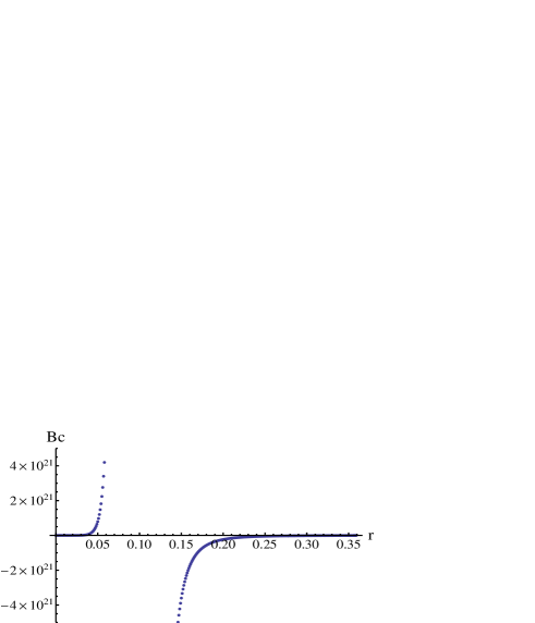
Figure 6: The dependence of $B_{C}$ on the reference point $r$ at different monolayer compressing speeds $V=10^{-15}$ (left), $10^{-1}$ (right) m/sec of the barrier for $t=0.01,\ \dot{\xi}=0.001,\ \dot{r}=0.01$ and $\dot{\phi}=0$.

The dependencies of $B_{C}$ on the particle velocity $v=\dot{r}/\dot{\xi}$ at the following monolayer compressing speeds $V=0.001,\ 0.1,\ 10.0$ for $\dot{r}=1.0,\ \dot{\phi}=0,\ t=0.01,\ r=0.1$, are shown in Fig. 7. One can see here (Fig. 7) that the increment of the compressing speed $V$ leads to the disappearing of the singularity of the function $B_{C}(v)$, while this singularity still reappears at some another location. The shift of the singularity towards the direction of larger values $v$ is a consequence of the disordering influence of the compressing barrier. Therefore the phase transition becomes enabled at some increment of the molecule velocity $v$.

The last one is in accordance with the experimental data presented in [39], and can be easily understood from the following explanation: while the speed $v$ of the particle increases, the bigger becomes the area occupied by the trajectory which is bent by the electro-capillary interaction, and there increases the probability of collisions between the particles of the monolayer, leading to the formation of structures.

Figure 7: Dependence of $B_{C}$ on the particle velocity $v=\dot{r}/\dot{\xi}$ at different monolayer compressing speeds: $V=0.001$ (red circles), $V=0.1$ (light blue triangles) and $V=10.0$ (dark blue squares) for $\dot{r}=1,\dot{\phi}=0,t=0.01,r=0.1$.

A)

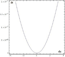
B)

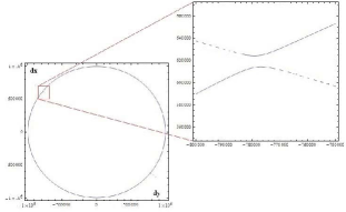
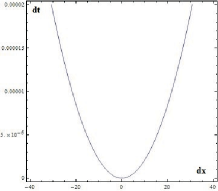
C)

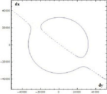
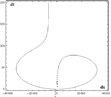
D)

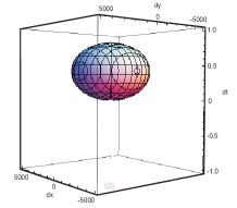
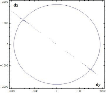
Figure 8: Projections of indicatrices (from the left) into the spatial (in the middle) and time–spatial (right) planes.

One can conclude according to the examination performed above that $B_{C}$ is an invariant for the monolayer structurization. Therefore, the Berwald scalar curvature $B_{C}$ – due to its invariance – allows us to classify indicatrices according to the behavior of $B_{C}$ in the following way. Figs. 1 and 2 illustrate eleven types of indicatrices – for large compression speed $V$ equal to 15.0. But the Berwald scalar curvature $B_{C}$ for corresponding indicatrices reveal the following descriptive classifying picture. It is easy to see observing the behavior of the scalar Berwald curvatures $B_{C}$ and the indicatrices corresponding to them in Figs. 1 and 2, that for $V=15.0$, $B_{C}$ may have one or two anomalies only. The second singularity occurs in a form of a stick-slip inversion of the first anomalous dependence $B_{C}=f(\dot{r})$ (see Fig. 2A). At the start of the compression process, the scalar curvature $B_{C}$ for the corresponding indicatrix has just one singularity (see Fig. 1), and afterwards the second singularity and another indicatrix which corresponds to a curvature $B_{C}$ having two singularities, appear (see Fig. 2). We note that in contrast to the numerically derived large diversity of indicatrices, their curvatures $B_{C}$ behave uniformly. One can distinguish two topological classes of indicatrices: (A – F) in Fig. 1 and (A – E) in Fig. 2, whose curvatures $B_{C}$ behave structurally different. The curvature $B_{C}$ everywhere vanishes, excluding anomalous areas similar to the phase transition areas. Therefore, one can conclude that the behavior of $B_{C}$ reflects several features of physically feasible processes, namely, the monolayer compression.

We further show that though there seemingly exist a large diversity of indicatrices attached to the Finsler structure, these basically classify into only three types of indicatrices, which topologically differ from each other. This can be established by the the peculiarities of the orthogonal projections of indicatrices to the spatial $\{x,\ y\}$ and to the time-spatial $\{x,\ t\}$ or $\{y,\ t\}$ planes. At very small speed $V$, $V\to 0$, $B_{C}$ vanishes identically, and the indicatrix tends to the one of the pseudo-Riemannian space for sufficiently large values of the reference radius $r$ (see Fig. 8A). The type of such indicatrix is referred as first type.

The indicatrices (A – F) in Fig. 1 are referred as indicatrices of second type. These indicatrices hold anomalous areas in the spatial plane (see Fig. 8B), and the relevant function $B_{C}$ exhibits one singularity.

The indicatrices (A – E) in Fig. 2 will be referred as indicatrices of third type. They hold anomalous areas both in spatial and time-spatial planes (see Fig. 8C and 8D), and the relevant function $B_{C}$ has two singularities.

We finally conclude that the monolayer is flat in the framework of Finsler geometry, and therefore the particles which move within it exhibit acceleration.

7 Conclusions

We proved that the curvature scalar $R_{c}$ is not an invariant of the monolayer, and this leads to its complex dependence on the monolayer parameters. On the contrary, $B_{c}$ vanishes for very small speeds, and is null as well outside certain domains of anomaly, for larger speeds of compression. Hence we conclude that the monolayer is flat in the framework of Finsler geometry, because the particles which move within it, exhibit acceleration. It is assumed that the domains of anomaly correspond to the phase transition and that the integral of $B_{c}$ represents the compressibility $\kappa$. It is shown that, in spite of the fact that the manifold of Finsler indicatrices seems to be large, still there exist only three types of indicatrices for the three types of dependence of the Berwald scalar curvature in terms of the tangent vector. These types can be identified by the three different projections on the spatial plane and on space-time plane. For small speeds – when $B_{c}$ is identically zero - the indicatrix tends to the one of the pseudo-Euclidean Minkowski space for rather large components of the reference point. The indicatrices which exhibit anomalies only in the spatial plane are characterized by having a singularity of $B_{c}$. The third type of indicatrices have two singularities for $B_{c}$, which corresponds to an anomalous behavior of the indicatrix both in the space and in the space-time planes.

As well, there are determined the Cartan tensor and the nonlinear Barthel connection, which provide means to estimate how far is the Finsler model from the pseudo-Euclidean one, and to construct Finsler adapted frames for the module of sections of the tangent bundle. Simulations illustrate this inter-relation for several classes of structure formation - which depend on compression speed and characteristics of the double electrical layer.

Vladimir Balan
University Politehnica of Bucharest, Splaiul Independentei 313,
060042 Bucharest, Romania, E-mail: vladimir.balan@upb.ro

Halina V. Grushevskaya and Nina G. Krylova
Faculty of Physics, Belarusan State University, 4 Nezavisimosti Ave.,
220030 Minsk, The Republic of Belarus, E-mail: grushevskaja@bsu.by , nina-kr@tut.by

Alexandru Oana
University Transilvania of Brasov, 50 Iuliu Maniu Str.,
500091 Brasov, Romania, E-mail: alexandruo@gmail.com

References

- [1] H.V. Krylova, Transport of Electrical Charge and Nonlinear Polarization into Periodically Packed Structures at Strong Electromagnetic Fields, Publishing Center of BSU, Minsk 2008.
- [2] I.P. Suzdalev, Nanotechnology: Physico-Chemistry of Nanoclusters, Librokom, Moscow 2009.
- [3] A.I. Drapeza, H.V. Grushevskaya, V. V. Hrushevsky, I. V. Lipnevich, T. I. Orekhovskaya, B. G. Shulitsky, Yu. M. Sudnik, G. N. Semenkova, N. G. Krylova, T. A. Kulahava, Nanosensing based on LB-CNT-clusters to register a functioning of membrane-dependent biological reactions, Proc. of Int. Conf. ”Optical Techniques and Nano-Tools for Material and Life Sciences” (ONT4MLS-2010), 15-19 June 2010, Minsk (Ed.: .N.Rubinov), 2010, vol. 2, 191–197.
- [4] V.M. Anishchik, N.N. Dorozhkin, H.V. Grushevskaya, V.V. Hrushevsky, G.G. Krylov, L.V.Kukharenko, and M.A. Senyuk, Dynamical instability of band structure for Fe-containing nanostructured Langmuir-Blodgett films, Proc. SPIE. 5219 (3003), 141–150.
- [5] K.B. Blodgett, Monomolecular films of fatty acids on glass, J. Amer. Chem. Soc. 56, 2 (1934), 495-495.
- [6] K.B. Blodgett, I.Langmuir, Built-up films of barium stearate and their optical properties, Phys. Rev. 51 (1937), 964-982.
- [7] C.Wöll, V.Vogel, Structural and dynamical properties of Langmuir-Blodgett crystals, in ”Adhesion and Friction” (Eds: M.Grunze and H.Kreuzer), Springer, Heidelberg 1989, 17-36.
- [8] D.K. Schwartz, Langmuir-Blodgett film structure, Surface Science Reports 27 (1997), 241–334.
- [9] H.V. Grushevskaya, George Krylov, and V.V. Hrushevsky, Kinetic theory of phase foliation at formation of Langmuir-Blodgett monolayers, J. Nonlin. Phenom. in Compl. Sys. 7, 1 (2004), 17–33.
- [10] W. da S. Robazzi, B. J. Mokross, Influence of interaction energy in fluid-fluid phase transitions on Langmuir monolayers, Brazilian J. Phys. 36, 3B (2006), 1013–1016.
- [11] D. Andelman, F. Brochard, C. Knobler and F. Rondelez, Structure and phase transitions in Langmuir monolayers, in ”Micelles, Membranes, Microemulsions and Monolayers” (Eds: W.M. Gelbart, A. Ben-Shaul, and D. Roux), Springer, Heidelberg 1994, 559–602.
- [12] S. Ramos, R. Castillo, Langmuir monolayers of C17, C19, and C21 fatty acids: textures, phase transitions, and localized oscillations, J. of Chem. Phys. 110, 14 (1999), 7021–7030.
- [13] H.V. Grushevskaya, N.G. Krylova, A Finsler geometrization of interactions at structure formation in Langmuir –Blodgett monolayers, Materials of 7th Int. Conf. on Non-Euclidean Geometry and its Applications, Cluj-Napoca, Romania, 5-9 July 2010, Babes-Bolyai University, Romania 2010, 29–29.
- [14] H.V. Grushevskaya, N.G. Krylova, Effects of Finsler geometry in physics surface phenomena: case of monolayer systems, HNGP, 1 (15), 8 (2011), 128–146.
- [15] P. Rashevski, Polymetric geometry, In: Proceedings of Seminar on vector and tensor analysis with its applications into geometry and physics, Vol. 5 (Ed.: V.F. Kagan), State Publishing Company of Technical and Theoretical Literature, Moscow, Leningrad 1941, 21–147.
- [16] H. Rund, Differential Geometry of Finsler Spaces, Scince Eds., Moscow 1981.
- [17] H.V. Grushevskaya and L.I. Gurskii, The technique of projecting operators in the theory of the reativistic wave equation on a non-compact group: the case of the charged vector bosone (in Russian), Proc.of BSUIR, 1, 2 (2003), 12-20; www.arXiv.org, quant-ph/0301176 (2003).
- [18] Gh. Atanasiu, V. Balan, N.Brinzei, M.Rahula, Second Order Differential Geometry and Applications: Miron-Atanasiu Theory (in Russian), Librokom Eds., Moscow 2010.
- [19] L.D. Landau, E.M. Lifshitz, Statistical Physics, part 1, In: Theoretical Physics, vol.5. (PhysMathLit, Moscow 2002). Pp.84-87
- [20] Le Bellac M., Mortessagne F., Batrouni G.G. Equilibrium and Non-Equilibrium Statistical Thermodynamics. (Cambridge University Press, 2004). P.31.
- [21] I.P. Bazarov. Thermodynamics. (High School, Moscow, 1991). P.129.
- [22] F. Weinhold. Metric geometry of equilibrium thermodynamics I, II, III, IV.// J. Chem. Phys. Vol. 63, P.2479, P.2484, P.2488, P.2496 (1975).
- [23] F. Weinhold. Metric geometry of equilibrium thermodynamics V. // J. Chem. Phys. Vol. 65, 558 (1976).
- [24] G. Ruppeiner. Thermodynamics: A Riemannian geometric model. // Phys. Rev. A. Vol. 20, 1608 (1979).
- [25] A. Bravetti, F. Nette. Second order phase transitions and thermodynamic geometry: a general approach // arXiv: 1208.0399v2 [math-ph] 22 Aug 2012.].
- [26] H. Quevedo. Geometrothermodynamics.// J. Math. Phys. Vol.48, 013506 (2007).
- [27] K. Binder. Theory of first-order phase transitions // Rep. Prog. Phys. Vol.50 (1987) 783-859.
- [28] G. Lippman, Relations entre les ph enomènes electriques et capillaries, Ann. Chim. Phys. 5 (1875), 494–549.
- [29] A. Frumkin, Couche Double. Electrocapillarite, Paris: Herman et Cie, Actual. Sci. Ind. 373, 1936.
- [30] L.D. Landau, E.M. Lifshitz, Electrodynamics of Continuous Media, In: Theoretical Physics, vol.8, Science, Moscow 1982.
- [31] J.W. Gibbs, The Collected Works of J. Willard Gibbs, vol.1, Longmans, Green & co., New York 1931.
- [32] H. Rund, Theory of curvature in Finsler spaces, Coll. Topologie Strasbourg, no. 4 (1951). (La Bibliotheque Nationale et Universitaire de Strasbourg, 1952); H.Rund, Eine Krümmungstheorie der Finslerschen Räume, Math. Ann. 125 (1952), 1–18.
- [33] P.A.M. Dirac, Lectures on quantum field theory. (Publising House ”LIBROKOM”, Moscow, 2009).
- [34] L. D. Landau, E.M. Lifshitz, Field Theory, In: Theoretical Physics, vol.2. (Science, Moscow, 1988).
- [35] Zhongmin Shen, Lectures on Finsler geometry, World Scientific, 2001.
- [36] V.Balan, I.R.Nicola, Berwald-Moor metrics and structural stability of conformally-deformed geodesic SODE, Appl. Sci. 11 (2009), 19-34.
- [37] M. Matsumoto, H. Shimada, On Finsler spaces with 1-form metric II: Berwald – Moor’s metric =(…, Tensor 32, 2 (1978), 275–278.
- [38] G. I. Garas’ko, Basics of Finsler Geometry for Physicists, Tetru Eds., Moscow 2009.
- [39] V.V. Hrushevsky, H.V. Krylova, Thermodynamics of phase states in Langmuir – Blodgett monolayers, In: Low-dimensional systems-2. No. 4 (Eds.: S.A. Maskevich et al.), Grodno State University, Grodno 2005, 30–36.