Additive-State-Decomposition Dynamic Inversion Stabilized Control for a Class of Uncertain MIMO Systems

Abstract

This paper presents a new control, namely additive-state-decomposition dynamic inversion stabilized control, that is used to stabilize a class of multi-input multi-output (MIMO) systems subject to nonparametric time-varying uncertainties with respect to both state and input. By additive state decomposition and a new definition of output, the considered uncertain system is transformed into a minimum-phase uncertainty-free system with relative degree one, in which all uncertainties are lumped into a new disturbance at the output. Subsequently, dynamic inversion control is applied to reject the lumped disturbance. Performance analysis of the resulting closed-loop dynamics shows that the stability can be ensured. Finally, to demonstrate its effectiveness, the proposed control is applied to two existing problems by numerical simulation. Furthermore, in order to show its practicability, the proposed control is also performed on a real quadrotor to stabilize its attitude when its inertia moment matrix is subject to a large uncertainty.

I Introduction

Stabilization in control systems with uncertainties depending on state and input has attracted the interest of many researchers. Uncertainties depending on state originate from various sources, including variations in plant parameters and inaccuracies that arise from identification. Input uncertainties include uncertain gains, dead zone nonlinearities, quantization, and backlash. In practice, these uncertainties may degrade or destabilize system performance. For example, given that aerodynamic parameters are functions of flight conditions, some aircraft are nonlinear and undergo rapid parameter variations. These attributes stem from the fact that aircraft can operate in a wide range of aerodynamic conditions. As a result, aerodynamic parameters, which exist in system and input matrices [1],[2],[3], are inherently uncertain. Therefore, robust stabilization control problems for systems with uncertainties depending on both state and input are important.

In this paper, a stabilization control problem is investigated for a class of multi-input multi-output (MIMO) systems subject to nonparametric time-varying uncertainties with respect to both state and input. Several accepted control methods for handling uncertainties are briefly reviewed. A direct approach is to estimate all unknown parameters, and then simultaneously use such parameters to resolve uncertainties. Lyapunov methods are adopted in analyzing the stability of closed-loop systems. In [3], nonparametric uncertainties involving state and input are approximated via basis functions with unknown parameters, which are estimated by given adaptive laws. With the estimated parameters, an approximate dynamic inversion method was proposed. It is in fact an adaptive dynamic inversion method [4],[5]. In [6], $\mathcal{L}_{1}$ adaptive control architecture was proposed for systems with an unknown input gain, as well as unknown time-varying parameters and disturbances. In [7], adaptive feedback control was used to track the desired angular velocity trajectory of a planar rigid body with unknown rotational inertia and unknown input nonlinearity. In [8], two asymptotic tracking controllers were designed for the output tracking of an aircraft system under parametric uncertainties and unknown nonlinear disturbances, which are not linearly parameterizable. An adaptive extension was then presented, in which the feedforward adaptive estimates of input uncertainties are used. As indicated in [3]-[8], adaptive controllers may require numerous integrators that correspond to unknown parameters in an uncertain system. Each unknown parameter requires an integrator for estimation, thereby resulting in a closed-loop system with a reduced stability margin. In addition, the estimates may not approach real parameters without the persistent excitation of signals, which are difficult to generate in practice, particularly under numerous unknown parameters [9]. The second direct method for resolving uncertainties is designing inverse control by a neural network that cancels input nonlinearities, thereby generating a linear function [10],[11]. In contrast to traditional inverse control schemes, a neural network approximates an unknown nonlinear term [12]. Neural network methods can also be considered as adaptive control methods, except that they have different basis functions. Thus, they also have the same problems as those encountered in adaptive control methods. The third approach is adopting sliding mode control, which presents inherent fast response and insensitivity to plant parameter variation and/or external perturbation. In [13], a new sliding mode control law based on the measurability of all system states was presented. The law ensures global reach conditions of the sliding mode for systems subject to nonparametric time-varying uncertainties with respect to both state and input. Along this idea of [13], an output feedback controller was further proposed in [14]. Sliding mode controllers essentially rely on infinite gains to achieve good tracking performance, which is not always feasible in practice. In practice, moreover, switching will consume energy and may excite high-frequency modes.

To overcome these drawbacks, this paper proposes a stabilization approach that involves dynamic inversion based on additive state decomposition (ASD). Additive state decomposition [15] is different from the lower-order subsystem decomposition methods existing in the literature. Concretely, taking the system $\dot{x}\left(t\right)=f\left(t,x\right),x\in\mathbb{R}^{n}$ for example, it is decomposed into two subsystems: $\dot{x}_{1}\left(t\right)=f_{1}\left(t,x_{1},x_{2}\right)$ and $\dot{x}_{2}\left(t\right)=f_{2}\left(t,x_{1},x_{2}\right)$, where $x_{1}\in\mathbb{R}^{n_{1}}\$and$\ x_{2}\in\mathbb{R}^{n_{2}},$ respectively. The lower-order subsystem decomposition satisfies $n=n_{1}+n_{2}$ and $x=x_{1}\oplus x_{2}.$ By contrast, the proposed additive state decomposition satisfies $n=n_{1}=n_{2}$ and$\ x=x_{1}+x_{2}.$ The key idea of the proposed method is that it combines nonparametric time-varying uncertainties with respect to both state and input into one disturbance by ASD. Such a disturbance is then compensated for. The proposed controller is continuous and enables asymptotic stability in the presence of time-invariant uncertainties. Moreover, by choosing a special filter, the proposed controllers can be finally replaced by proportional-integral (PI) controllers. This is consistent with the controller form in [16] for a similar problem. However, compared with [16], the considered plant, analysis method and design procedure are all different, especially the analysis method and design procedure. The bound on a parameter, corresponding to the singular perturbation parameter in [16], is also given explicitly. Moreover, our proposed controllers are not just in the form of PI controllers. This paper focuses on a stabilization problem, which distinguishes it from the authors’ previous work on ASD. In previous research, ASD has been applied to tracking problems for nonlinear systems without stabilization problems or with the stabilization problem being solved by a simple state feedback controller [17],[18],[19]. The other additive decomposition, namely additive output decomposition [20], is also applied to a tracking problem with a stable controlled plant.

II Problem Formulation and Additive State Decomposition

II-A Problem Formulation

Consider a class of MIMO systems subject to nonparametric time-varying uncertainties with respect to both state and input as follows:

$$\dot{x}\left(t\right)=A_{0}x\left(t\right)+B\left(h\left(t,u\right)+\sigma\left(t,x\right)\right),x\left(0\right)=x_{0}$$ (1)

where $x\left(t\right)\in\mathbb{R}^{n}$ is the system state (taken as a measurable output), $u\left(t\right)\in\mathbb{R}^{m}$ is the control, $A_{0}\in\mathbb{R}^{n\times n}$ is a known matrix, $B\in\mathbb{R}^{n\times m}$ is a known constant matrix, $h:\left[0,\infty\right)\times\mathbb{R}^{m}\rightarrow\mathbb{R}^{m}$ is an unknown nonlinear vector function, and $\sigma:\left[0,\infty\right)\times\mathbb{R}^{n}\rightarrow\mathbb{R}^{m}$ is an unknown nonlinear time-varying disturbance. For system (1), the following assumptions are made.

Assumption 1. The pair $\left(A_{0},B\right)$ is controllable.

Assumption 2. The unknown nonlinear vector function$\ h$ satisfies $h\left(t,0\right)\equiv 0,\ \left\|\frac{\partial h}{\partial t}\right\|\leq l_{h_{t}}\left\|u\right\|,$ $\frac{\partial h}{\partial u}>\underline{l}_{h_{u}}I_{m}$ and $\left\|\frac{\partial h}{\partial u}\right\|\leq\overline{l}_{h_{u}},$ $\forall u\in\mathbb{R}^{m},$ $\forall t\geq 0,$ where $l_{h_{t}},\underline{l}_{h_{u}},\overline{l}_{h_{u}}>0.$

Assumption 3. The time-varying disturbance$\ \sigma\left(t,x\right)$ satisfies $\left\|\sigma\left(t,x\right)\right\|\leq k_{\sigma}\left\|x\left(t\right)\right\|+\delta_{\sigma}\left(t\right),\ \left\|\frac{\partial\sigma}{\partial x}\right\|\leq l_{\sigma_{x}}$ and $\left\|\frac{\partial\sigma}{\partial t}\right\|\leq l_{\sigma_{t}}\left\|x\left(t\right)\right\|+d_{\sigma}\left(t\right),$ where $\frac{\partial\sigma}{\partial x}\in\mathbb{R}^{m\times n},$ $k_{\sigma},\delta_{\sigma}\left(t\right),l_{\sigma_{x}},l_{\sigma_{t}},d_{\sigma}\left(t\right)>0,$ $\forall t\geq 0$, and $\delta_{\sigma}\left(t\right),d_{\sigma}\left(t\right)$ are bounded.

Remark 1. If $h$ is a dead zone function such as $h\left(t,u\right)=\left\{\begin{array}[c]{c}u\\ 0\end{array}\right.\begin{array}[c]{c}\left|u_{i}\right|\geq\mu,i=1,\cdots,m\\ \left|u_{i}\right|<\mu,i=1,\cdots,m\end{array}$, then it can be reformulated as $h\left(t,u\right)=u+\delta\left(t\right),$ where $\left\|\delta\left(t\right)\right\|\leq\mu.$ In practice, the parameters $l_{h_{t}},\underline{l}_{h_{u}},\overline{l}_{h_{u}},k_{\sigma},\delta_{\sigma},l_{\sigma_{x}},l_{\sigma_{t}},d_{\sigma}\$need not be known.

The control objective is to design a stabilized controller to drive the system state such that $x\left(t\right)\rightarrow 0$ as $t\rightarrow\infty$ or the state is ultimately bounded by a small value. In the following, for convenience, the notation $t$ will be dropped except when necessary for clarity.

II-B Additive State Decomposition

In order to make the paper self-contained, ASD in [15],[17],[18],[19] is recalled briefly here. Consider the following ‘original’ system:

$$f\left({t,\dot{x},x}\right)=0,x\left(0\right)=x_{0}$$ (2)

where $x\in\mathbb{R}^{n}$. First, a ‘primary’ system is brought in, having the same dimension as (2):

$$f_{p}\left({t,\dot{x}_{p},x_{p}}\right)=0,x{{}_{p}}\left(0\right)=x_{p,0}$$ (3)

where ${x_{p}}\in\mathbb{R}^{n}$. From the original system (2) and the primary system (3), the following ‘secondary’ system is derived:

$$f\left({t,\dot{x},x}\right)-f_{p}\left({t,\dot{x}_{p},x_{p}}\right)=0,x\left(0\right)=x_{0}$$ (4)

where ${x_{p}}\in\mathbb{R}^{n}$ is given by the primary system (3). A new variable ${x_{s}}\in\mathbb{R}^{n}$ is defined as follows:

$${x_{s}\triangleq x-x_{p}}.$$ (5)

Then the secondary system (4) can be further written as follows:

$$f\left({t,\dot{x}_{s}+\dot{x}_{p},x_{s}+x_{p}}\right)-f_{p}\left({t,\dot{x}_{p},x_{p}}\right)=0,x{{}_{s}}\left(0\right)=x_{0}-x_{p,0}.$$ (6)

From the definition (5), it follows

$${x}\left(t\right)={x_{p}\left(t\right)+x_{s}\left(t\right),t\geq 0.}$$ (7)

Remark 2. By ASD, the system (2) is decomposed into two subsystems with the same dimension as the original system. In this sense our decomposition is “additive”. In addition, this decomposition is with respect to state. So, it is called “additive state decomposition”.

As a special case of (2), a class of differential dynamic systems is considered as follows:

$$\dot{x} =f\left({t,x}\right),x\left(0\right)=x_{0},$$

$$y =g\left({t,x}\right)$$ (8)

where ${x}\in\mathbb{R}^{n}$ and $y\in\mathbb{R}^{m}.$ Two systems, denoted by the primary system and (derived) secondary system respectively, are defined as follows:

$$\dot{x}_{p} =f_{p}\left({t,x_{p}}\right),x_{p}\left(0\right)=x_{p,0}$$

$$y_{p} =g_{p}\left({t,x}_{p}\right)$$ (9)

and

$$\dot{x}_{s} =f\left({t,x_{p}}+{x_{s}}\right)-f_{p}\left({t,x_{p}}\right),x_{s}\left(0\right)=x_{0}-x_{p,0},$$

$$y_{s} =g\left({t,x_{p}}+{x_{s}}\right)-g_{p}\left({t,x}_{p}\right)$$ (10)

where ${x_{s}}\triangleq{x-x_{p}}$ and $y_{s}\triangleq{y-y_{p}}$. The secondary system (10) is determined by the original system (8) and the primary system (9). From the definition, it follows

$${x}\left(t\right)={x_{p}\left(t\right)+x_{s}\left(t\right),y\left(t\right)=y_{p}\left(t\right)+y_{s}\left(t\right),t\geq 0.}$$ (11)

III Additive-State-Decomposition Dynamic Inversion Stabilized Control

In this section, by ASD, the considered uncertain system is first transformed into an uncertainty-free system but subject to a lumped disturbance at the output. Then a dynamic inversion method is applied to this transformed system. Finally, the performance of the resultant closed-loop system is analyzed.

III-A Output Matrix Redefinition

Since the pair $\left(A_{0},B\right)$ is controllable by Assumption 1, a vector $K\in\mathbb{R}^{n\times m}$ can be always found such that $A_{0}+BK^{T}$ is stable. This also implies that there exist $0<P,M\in\mathbb{R}^{n\times n}$ such that

$$P\left(A_{0}+BK^{T}\right)+\left(A_{0}+BK^{T}\right)^{T}P=-M.$$ (12)

According to this, the system (1) is rewritten to be

$$\dot{x}=Ax+B\left(h\left(t,u\right)-K^{T}x+\sigma\left(t,x\right)\right),x\left(0\right)=x_{0}$$ (13)

where $A=A_{0}+BK^{T}.$ Based on matrix $A$, a new definition of output matrix $C$ is given in the following theorem.

Theorem 1. Under Assumption 1, suppose $A^{T}$ has $n$ negative real eigenvalues, denoted by $-\lambda_{i}\in\mathbb{R},$ to which correspond $n$ independent unit real eigenvectors, denoted by $c_{i}\in\mathbb{R}^{n},$ $i=1,\cdots,n.$ If the output matrix is proposed as

$$C=\left[\begin{array}[c]{ccc}c_{1}&\cdots&c_{m}\end{array}\right]\in\mathbb{R}^{n\times m}$$ (14)

then

$$C^{T}A=-\Lambda C^{T}$$

where $\Lambda=$diag$\left(\lambda_{1},\cdots,\lambda_{m}\right)\in\mathbb{R}^{m\times m}.$ Furthermore, if $\Lambda$ has the form $\Lambda=\alpha I_{m},$ then det$\left(C^{T}B\right)\neq 0.$

Proof. Since $c_{i},$ $i=1,\cdots,m$ are $m$ independent unit eigenvectors of $A^{T}$, it follows

$$A^{T}c_{i}=-\lambda_{i}c_{i},i=1,\cdots,m,$$

namely $A^{T}C=-C\Lambda$. Then $C^{T}A=-\Lambda C^{T}.$ Next, det$\left(C^{T}B\right)\neq 0\$will be shown. Suppose, to the contrary, that det$\left(C^{T}B\right)=0.$ According to this, there exists a nonzero vector $w\in\mathbb{R}^{m}$ such that $w^{T}C^{T}B=0.$ Define $v=Cw.$ Since $w\neq 0$ and $C\$is of column full rank, it follows $v\neq 0.$ With such a vector $v,$ it further follows

$$v^{T}\left[\begin{array}[c]{cccc}B&AB&\cdots&A^{n-1}B\end{array}\right] =w^{T}C^{T}\left[\begin{array}[c]{cccc}B&AB&\cdots&A^{n-1}B\end{array}\right]$$

$$=w^{T}\left[\begin{array}[c]{cccc}C^{T}B&C^{T}AB&\cdots&C^{T}A^{n-1}B\end{array}\right]$$

$$=w^{T}\left[\begin{array}[c]{cccc}C^{T}B&-\alpha C^{T}B&\cdots&\left(-\alpha\right)^{n-1}C^{T}B\end{array}\right]$$

$$=w^{T}C^{T}B\left[\begin{array}[c]{cccc}I_{m}&-\alpha I_{m}&\cdots&\left(-\alpha\right)^{n-1}I_{m}\end{array}\right]$$

$$=0.$$

This implies that rank$\left[\begin{array}[c]{cccc}B&AB&\cdots&A^{n-1}B\end{array}\right]<n,$ namely $\left(A,B\right)$ is uncontrollable and $\left(A_{0},B\right)$ is further uncontrollable, which contradicts the assumption that the pair $\left(A_{0},B\right)$ is controllable. Then det$\left(C^{T}B\right)\neq 0.$ $\square$

By Theorem 1, a virtual output $y=C^{T}x\$is defined, whose first derivative is

$$\dot{y} =C^{T}\dot{x}$$

$$=C^{T}Ax+C^{T}B\left(h\left(t,u\right)-K^{T}x+\sigma\left(t,x\right)\right)$$

$$=-\Lambda y+C^{T}B\left(h\left(t,u\right)-K^{T}x+\sigma\left(t,x\right)\right).$$ (15)

Then, the system (13) can be rewritten as

$$\left[\begin{array}[c]{c}\dot{\eta}\\ \dot{y}\end{array}\right]=\left[\begin{array}[c]{cc}A_{\eta}&B_{\eta}\\ 0_{m\times\left(n-m\right)}&-\Lambda\end{array}\right]\left[\begin{array}[c]{c}\eta\\ y\end{array}\right]+\left[\begin{array}[c]{c}0_{\left(n-m\right)\times\left(n-m\right)}\\ C^{T}B\end{array}\right]\left(h\left(t,u\right)-K^{T}x+\sigma\left(t,x\right)\right)$$ (16)

where $\eta\in\mathbb{R}^{n-m}$ is an internal part and $y\in\mathbb{R}^{m}$ is an external part. Since $A$ is stable, $A_{\eta}\in\mathbb{R}^{\left(n-m\right)\times\left(n-m\right)}$ is stable too. In fact, a minimum-phase MIMO system is designed by the new output matrix.

III-B Additive State Decomposition

Consider the system (15) as the original system. The primary system is chosen as follows:

$$\dot{y}_{p}=-\Lambda y_{p}+C^{T}Bu,y_{p}\left(0\right)=0.$$ (17)

Then the secondary system is determined by the original system (13) and the primary system (17) with the rule (10), resulting in

$$\dot{y}_{s}=-\Lambda y_{s}+C^{T}B\left(-u+h\left(t,u\right)-K^{T}\left({x}\right)+\sigma\left(t,{x}\right)\right),y_{s}\left(0\right)=C^{T}x_{0}.$$ (18)

According to (11), it follows

$$y=y_{p}+y_{s}.$$ (19)

Define a transfer function $G\left(s\right)=\left(sI_{m}+\Lambda\right)^{-1}C^{T}B.$ Then, rearranging (17)-(19) results in

$$\dot{y}_{p} =-\Lambda y_{p}+C^{T}Bu,y_{p}\left(0\right)=0.$$

$$y =y_{p}+d_{l}$$ (20)

where $d_{l}$ $=$ $C^{T}x_{s}$ $=G\left(-u+h\left(t,u\right)-K^{T}x+\sigma\left(t,x\right)\right)+e^{-\Lambda t}C^{T}x_{0}\$is called the lumped disturbance. Furthermore, (20) is written as

$$y=Gu+d_{l}.$$ (21)

The lumped disturbance $d_{l}$ includes uncertainties, disturbance and input. Fortunately, since $y_{p}=Gu$ and the output $y$ are known, the lumped disturbance $d_{l}$ can be observed exactly by

$$\hat{d}_{l}=y-Gu.$$ (22)

It is easy to see that $\hat{d}_{l}\equiv d_{l}.$

III-C Dynamic Inversion Control

So far, by ASD, the uncertain system (1) has been transformed into an uncertainty-free system (21) but subject to a lumped disturbance, which is shown in Fig.1.

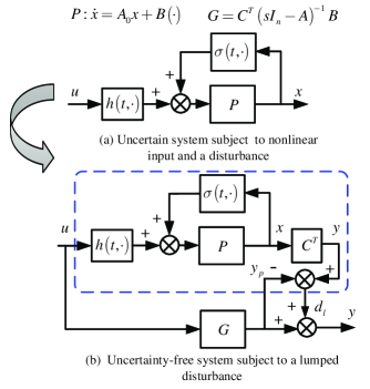
Figure 1: Model Transformation

For the system (21), since $G$ is minimum-phase and known, the dynamic inversion tracking controller design is represented as follows:

$$u=-G^{-1}\hat{d}_{l}.$$ (23)

Substituting (23) into (21) results in

$$y =-GG^{-1}\hat{d}_{l}+d_{l}$$

$$=-\hat{d}_{l}+d_{l}=0$$

where $\hat{d}\equiv d_{l}$ is utilized. As a result, perfect tracking is achieved. However, the proposed controller (23) cannot be realized. By introducing a low-pass filter matrix $Q$, the controller (23) is modified as follows:

$$u=-QG^{-1}\hat{d}_{l}$$ (24)

which has the simple structure shown in Fig.2. Furthermore, substituting (22) into (24) results in

$$u=-QG^{-1}\left(y-Gu\right).$$

Then, it can be further written as

$$u=-\left(I_{m}-Q\right)^{-1}QG^{-1}C^{T}x$$ (25)

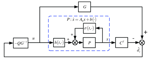
Figure 2: Structure of the ASD Dynamic Inversion Stabilized Controller

If det$\left(C^{T}B\right)\neq 0$, then the controller above is realizable. By employing the controller (24), the output becomes

$$y=\left(I_{m}-Q\right)\hat{d}_{l}.$$ (26)

Since $Q$ is a low-pass filter matrix, and the low-frequency range is often dominant in a signal, it is expected that the output will be attenuated by the transfer function $I_{m}-Q$. A detailed analysis is given in the following section.

Remark 3. By the proposed output matrix redefinition, the considered MIMO uncertainty system is transformed into a MIMO minimum-phase system with relative degree one. By ASD, it is further transformed into a simple transfer function, namely (21). Owing to the simple transfer function, the controller design for (21) is straightforward by the idea of dynamic inversion.

III-D Performance Analysis

Since the lumped disturbance $d_{l}$ involves the input $u$, the resultant closed-loop system may be unstable. Next, some conditions are given to guarantee that the control input $u$ is bounded. Substituting $\hat{d}_{l}$ into (24) results in

$$u =-QG^{-1}\left[G\left(-u+h\left(t,u\right)-K^{T}x+\sigma\left(t,x\right)\right)+e^{-\Lambda t}C^{T}x_{0}\right]$$

$$=Q\left(u-h\left(t,u\right)+K^{T}x-\sigma\left(t,x\right)\right)-QG^{-1}e^{-\Lambda t}C^{T}x_{0}.$$ (27)

Multiplying $Q^{-1}$ on both sides of (27) yields

$$Q^{-1}u=u-h\left(t,u\right)+K^{T}x-\sigma\left(t,x\right)+\xi$$ (28)

where $\xi=-G^{-1}e^{-\Lambda t}C^{T}x_{0}$. Since $G=\left(sI_{m}+\Lambda\right)^{-1}C^{T}B$, the term $\xi$ will tend to zero exponentially. A simple way is to choose $Q=\frac{1}{\epsilon s+1},$ where $\epsilon>0$ can be considered as a singular perturbation parameter. By the filter $Q$, (28) is further written as

$$\epsilon\dot{u}=-h\left(t,u\right)+K^{T}x-\sigma\left(t,x\right)+\xi.$$ (29)

The following theorem will give an explicit bound on $\epsilon$, below which the stability of closed-loop dynamics forming by (13) and (29) can be guaranteed.

Theorem 2. Suppose i) Assumptions 1-3 hold, ii) the controller is designed as (24) with $Q=\frac{1}{\epsilon s+1},$ iii) $\epsilon$ satisfies

$$0<\epsilon<\frac{\underline{l}_{h_{u}}}{\gamma_{1}+\frac{2}{\gamma_{0}}\left(\gamma_{2}+l_{\sigma_{t}}\right)^{2}}$$ (30)

where

$$\gamma_{0} =\lambda_{\min}\left(M\right)$$

$$\gamma_{1} =2\left(\left\|K\right\|+l_{\sigma_{x}}\right)\left\|b\right\|+2\frac{l_{h_{t}}}{\underline{l}_{h_{u}}}$$

$$\gamma_{2} =\left\|P\right\|\left\|b\right\|+\left\|A\right\|\left(\left\|K\right\|+l_{\sigma_{x}}\right)+\left\|K\right\|+k_{\sigma}.$$ (31)

Then the state of system (1) is uniformly ultimately bounded with respect to the bound $\sqrt{\frac{1}{\eta\left(\epsilon\right)}\frac{\epsilon}{\underline{l}_{h_{u}}}}\left(\frac{l_{h_{t}}}{\underline{l}_{h_{u}}}\delta_{\sigma}+d_{\sigma}\right),$ where $\eta\left(\epsilon\right)=\min(\frac{\gamma_{0}}{2\lambda_{\max}\left(P\right)},\frac{1}{\epsilon}\underline{l}_{h_{u}}-\gamma_{1}-\frac{2}{\gamma_{0}}\left(\gamma_{2}+l_{\sigma_{t}}\right)^{2}).$ Furthermore, if $l_{h_{t}}\delta_{\sigma}\left(t\right)\rightarrow 0$ and $d_{\sigma}\left(t\right)\rightarrow 0$, then the state $x\left(t\right)\rightarrow 0$ as $t\rightarrow\infty.$

Proof. See Appendix.

Remark 4. According to Theorem 2, if the uncertainties are time invariant, namely $l_{h_{t}}=0$ and $d_{\sigma}=0,$ then the proposed controller results in asymptotic stability. Also, from Theorem 2, a sufficiently small $\epsilon$ will satisfy (30) and the ultimate bound will be reduced by decreasing $\epsilon.$ However, it should be pointed out that a small $\epsilon$ in turn will result in a reduced stability of the closed-loop system, namely the roots are closer to the imaginary axis. For example, consider a simple situation where $h\left(t,u\right)=u\left(t-\tau\right).$ Given $\tau>0$, the dynamical system $\epsilon\dot{u}=-u\left(t-\tau\right)$ will lose stability on choosing a sufficiently small $\epsilon$ no matter how small the delay $\tau$ is (The characteristic equation of $\epsilon\dot{u}=-u\left(t-\tau\right)$ is $\epsilon s+e^{-s\tau}=0,$ which can be approximated by $\left(\epsilon-\tau\right)s+1=0.$ Therefore, one solution of the characteristic equation is $s\approx\frac{1}{\tau-\epsilon}.$ If $\epsilon<\tau$, then $s>0$, namely the dynamical system $\epsilon\dot{u}=-u\left(t-\tau\right)$ is unstable). Therefore, an appropriate $\epsilon>0\$should be chosen to achieve a tradeoff between tracking performance and robustness. The parameters $l_{h_{t}},\underline{l}_{h_{u}},\overline{l}_{h_{u}},k_{\sigma},\delta_{\sigma},l_{\sigma_{x}},l_{\sigma_{t}},d_{\sigma}$ need not be known, and $\epsilon$ is chosen as large as possible consistent with the state subject to an acceptable uniform ultimate bound according to practical requirements. From the above analysis, the design procedure is summarized as follows.

Procedure

Step 1 Design a state feedback gain $$K\in\mathbb{R}^{n\times m}$$ such that is stable with

negative real eigenvalues denoted by

Step 2 Define where are independent unit

eigenvectors corresponding to eigenvalues of respectively.

Step 3 Design (24) or (25) with and .

Step 4. Choose the appropriate in practice (see text).

        

IV Numerical Simulations

To demonstrate its effectiveness, the proposed control method is applied to two existing problems in [3],[13] for comparison by numerical simulations.

IV-A An Uncertain SISO System

As in [13], the following uncertain dynamics are considered

$$\dot{x}\left(t\right)=A_{0}x\left(t\right)+B\left(\Phi\left(u\left(t\right)\right)+e\left(x,t\right)\right)$$ (32)

where

$$A_{0} =\left[\begin{array}[c]{ccc}0&1&0\\ 0&0&1\\ -1&-3&-1\end{array}\right],B=\left[\begin{array}[c]{c}0\\ 0\\ 1\end{array}\right]$$

$$\Phi\left(u\left(t\right)\right) =\left(0.5+0.3\sin u\left(t\right)+e^{0.2\left|\cos u\left(t\right)\right|}\right)u\left(t\right)$$

$$e\left(x,t\right) =\left(0.3+0.2\cos x_{1}\right)\sqrt{x_{1}^{2}+x_{2}^{2}+x_{3}^{2}}-0.5\sin x_{2}$$

The objective is to drive $x\left(t\right)\rightarrow 0$ as $t\rightarrow\infty$.

For the dynamics (32), according to Procedure, the following design is given.

Step 1. According to the procedure, design $K=\left[\begin{array}[c]{ccc}-5&-8&-5\end{array}\right]^{T}$ resulting in $A=A_{0}+BK^{T}$ with $3$ different negative real eigenvalues $-1,-2,-3$.

Step 2. Selecting eigenvectors of $A^{T}$ corresponding to its eigenvalues $-1\$results in $C=\left[\begin{array}[c]{ccc}6&5&1\end{array}\right]^{T}.$

Step 3. Design controller $u=-QG^{-1}\hat{d}_{l}=-\frac{1}{\epsilon}\left(1+\frac{1}{s}\right)C^{T}x,$ where $G=\frac{1}{s+1}$,$\ Q=\frac{1}{\epsilon s+1},$ $\hat{d}_{l}=C^{T}x-Gu$.

Step 4. Choose $\epsilon=0.1.$

The range of the control input $u$ is chosen as $\left[-5,5\right]\$in practice. Driven by the designed controller, the control performance is shown in Fig. 3. As shown, all states converge to zero. Moreover, the control input is continuous and bounded. The control performance by the sliding mode controller proposed in [13] is shown in Fig. 4. The index $E\left(t\right)={\displaystyle\int\nolimits_{0}^{t}}\left|\dot{u}\left(s\right)\right|ds$ is introduced to represent the energy cost. It is easy to observe that our proposed controller saves more energy compared with the sliding mode controller proposed in [13].

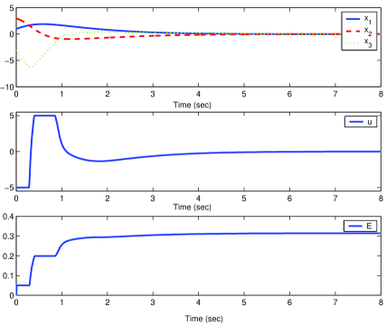
Figure 3: Stabilization Performance of the SISO Dynamics Driven by the ASD Dynamic Inversion Stabilized Controller

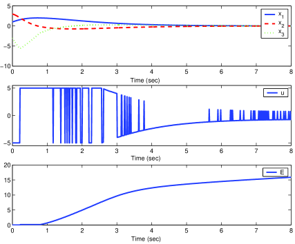
Figure 4: Stabilization Performance of the SISO Dynamics Driven by the Sliding Mode Controller Proposed in [10]

IV-B An Uncertain MIMO System

As in [3], the lateral/directional baseline model of an F-16 from [21] flying at sea level with an airspeed of $502$ $ft/s$ and angle of attack of $2.11$ deg is used. Denote the angle of sideslip, the roll angle, the stability axis roll and yaw rates, aileron and rudder control by $\beta,\phi,p_{s},r_{s},\delta_{a},\delta_{r}$ respectively. The full roll/yaw dynamics in state space form gives

$$\underset{\dot{x}\left(t\right)}{\underbrace{\left[\begin{array}[c]{c}\dot{\beta}\left(t\right)\\ \dot{\phi}\left(t\right)\\ \dot{p}_{s}\left(t\right)\\ \dot{r}_{s}\left(t\right)\end{array}\right]}}=A_{0}\underset{x\left(t\right)}{\underbrace{\left[\begin{array}[c]{c}\beta\left(t\right)\\ \phi\left(t\right)\\ p_{s}\left(t\right)\\ r_{s}\left(t\right)\end{array}\right]}}+B\left[\begin{array}[c]{c}\delta_{a}\left(t\right)+f_{1}\left(\beta\left(t\right),p_{s}\left(t\right),r_{s}\left(t\right),\delta_{a}\left(t\right)\right)\\ \delta_{r}\left(t\right)+f_{2}\left(\beta\left(t\right),p_{s}\left(t\right),r_{s}\left(t\right),\delta_{r}\left(t\right)\right)\end{array}\right].$$ (33)

Here

$$A_{0} =\left[\begin{array}[c]{cccc}-0.3220&0.064&0.0364&-0.9917\\ 0&0&1&0.0393\\ -30.6490&0&-3.6784&0.6646\\ 8.5395&0&-0.0254&-0.4764\end{array}\right],B=\left[\begin{array}[c]{cc}0&0\\ 0&0\\ -0.7331&0.1315\\ -0.0319&-0.0620\end{array}\right]$$

$$f_{1} =\left(\left(1-C_{1}\right)e^{-\frac{\left(\beta-\beta_{0}\right)^{2}}{2\sigma_{1}^{2}}}+C_{1}\right)\left(\tanh\left(\delta_{a}+h_{1}\right)+\tanh\left(\delta_{a}-h_{1}\right)+0.001\delta_{a}\right)$$

$$+D_{1}\cos\left(A_{1}p_{s}-\omega_{1}\right)\sin\left(A_{2}r_{s}-\omega_{2}\right)+D_{2}$$

$$f_{2} =\left(\left(1-C_{2}\right)e^{-\frac{\left(\beta-\beta_{0}\right)^{2}}{2\sigma_{2}^{2}}}+C_{2}\right)\left(\tanh\left(\delta_{r}+h_{2}\right)+\tanh\left(\delta_{a}-h_{2}\right)+0.001\delta_{r}\right)$$

$$+D_{3}\cos\left(A_{3}p_{s}-\omega_{3}\right)\sin\left(A_{4}r_{s}-\omega_{4}\right)+D_{4}.$$

where $A_{1}=0.33,$ $A_{2}=0.195,$ $A_{3}=0.45,$ $A_{4}=1.85,$ $D_{1}=0.295,$ $D_{2}=-0.0865,$ $D_{3}=0.055,$ $D_{4}=-0.007,$ $w_{1}=1.6,$ $w_{2}=0,$ $w_{3}=-1.9,$ $w_{4}=0,$ $C_{1}=0.3,$ $C_{2}=0.3,$ $h_{1}=7,$ $h_{2}=2.7,$ $\delta_{1}=0.25,$ $\delta_{2}=0.25,$ $\beta_{0}=0.$ Readers are refered to [3] for details. The dynamics (33) can be formulated as (1). The objective is to drive $x\left(t\right)\rightarrow 0$ as $t\rightarrow\infty$.

For the dynamics (33), according to the design procedure at the end of Section III.C, the following design is given.

Step 1. According to the procedure, design

$$K=\left[\begin{array}[c]{cc}-27.5037&93.4020\\ 14.2953&35.0244\\ 4.5010&13.9005\\ 12.7039&58.8096\end{array}\right]$$

resulting in $A=A_{0}+BK^{T}$ with the $4$ negative real eigenvalues $-1,-2,-3,-4$.

Step 2. Selecting eigenvectors of $A^{T}$ corresponding to its eigenvalues $-1,-2\$results in

$$C=\left[\begin{array}[c]{cc}0.6537&-0.5473\\ 0.6819&0.7985\\ 0.2285&0.1961\\ -0.2354&0.1561\end{array}\right].$$

Step 3. Design controller

$$u=\left[\begin{array}[c]{c}\delta_{a}\\ \delta_{r}\end{array}\right]=-QG^{-1}\hat{d}_{l}=-\left(C^{T}B\right)^{-1}\left[\begin{array}[c]{cc}\frac{s+1}{\epsilon s}&0\\ 0&\frac{s+2}{\epsilon s}\end{array}\right]C^{T}x$$ (34)

where $G=\left[\begin{array}[c]{cc}\frac{1}{s+1}&0\\ 0&\frac{1}{s+2}\end{array}\right]C^{T}B$,$\ Q=\frac{1}{\epsilon s+1},$ $\hat{d}_{l}=C^{T}x-Gu$.

Step 4. Choose the appropriate $\epsilon=0.2.$

The range of the control input $\delta_{a},\delta_{r}$ is chosen as $\left[-20\deg,20\deg\right]\$in practice. Driven by (34), the control performance is shown in Fig. 5. As shown, all states converge to zero. Moreover, the control input is continuous and bounded. Here the information of nonlinear terms $f_{1}$ and $f_{2}$ is not required, let alone learn the parameters. So, compared with controller proposed in [3], the controller design and controller structure are both simpler.

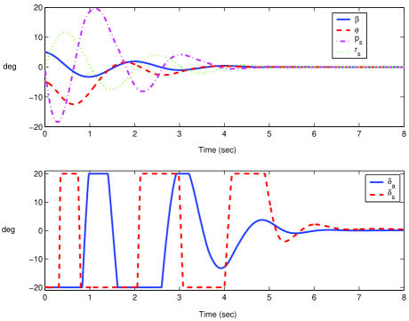
Figure 5: Stabilization Performance of F-16 Roll/Yaw Dynamics Driven by the ASD Dynamic Inversion Stabilized Controller

V An Application: Attitude Control of A Quadrotor

In this section, in order to show its practicability, the proposed ASD dynamic inversion stabilized controller is applied to attitude control of a quadrotor when its inertia moment matrix is subject to a large uncertainty.

V-A Problem Formulation

By taking actuator dynamics into account, the linear roll model of the quadrotor around hover conditions is

$$\underset{\dot{x}_{\phi}}{\underbrace{\left[\begin{array}[c]{c}\dot{\phi}\left(t\right)\\ \dot{p}\left(t\right)\\ \dot{L}\left(t\right)\end{array}\right]}}=\underset{A_{0}}{\underbrace{\left[\begin{array}[c]{ccc}0&1&0\\ 0&0&1\\ 0&0&-\omega\end{array}\right]}}\underset{x_{\phi}}{\underbrace{\left[\begin{array}[c]{c}\phi\left(t\right)\\ p\left(t\right)\\ L\left(t\right)\end{array}\right]}}+\underset{B_{0}}{\underbrace{\left[\begin{array}[c]{c}0\\ 0\\ \omega\end{array}\right]}}J_{\phi}^{-1}\tau_{\phi}$$ (35)

where $\omega$ is the actuator bandwidth, $\tau_{\phi}$ is the command torque to be selected, and $x_{\phi}=\left[\begin{array}[c]{ccc}\phi&p&L\end{array}\right]^{T}\in\mathbb{R}^{3}\$with $\phi,p,L\in\mathbb{R}$ being the angle, angular velocity and torque of the roll channel in the body-fixed frame, respectively. In practice, $\phi,p$ can be measured but $L$ cannot be. According to this, $L$ is estimated by $\dot{\hat{L}}=-\omega\hat{L}+\omega\tau_{\phi},\hat{L}\left(0\right)=0,$ taken as the true measurement for simplicity. In this sense, $x_{\phi}$ is known. Let $J\in\mathbb{R}^{3\times 3}$ be the inertia moment matrix of the quadrotor, $x_{\theta}=\left[\begin{array}[c]{ccc}\theta&q&M\end{array}\right]^{T}\in\mathbb{R}^{3}$ and$\ x_{\psi}=\left[\begin{array}[c]{ccc}\theta&q&N\end{array}\right]^{T}\in\mathbb{R}^{3}.$ Here $\theta,\psi\in\mathbb{R}$ are pitch and yaw angle respectively, while $q,r$ are respectively their angular velocity in the body-fixed frame. The torques $M,N\in\mathbb{R}\$represent the airframe pitch and yaw torque, respectively. Similar to (35), the linear attitude model of the quadrotor is expressed as

$$\dot{x}=\bar{A}_{0}x+BJ^{-1}\tau,x\left(0\right)=x_{0}.$$ (36)

Here $x=\left[\begin{array}[c]{ccc}x_{\phi}&x_{\theta}&x_{\psi}\end{array}\right]^{T}\in\mathbb{R}^{9}$ is the state and $\tau=\left[\begin{array}[c]{ccc}\tau_{\phi}&\tau_{\theta}&\tau_{\psi}\end{array}\right]^{T}\in\mathbb{R}^{3}.$ The system matrix and input matrix in (36) are

$$\bar{A}_{0}=\left[\begin{array}[c]{ccc}A_{0}&0_{3\times 3}&0_{3\times 3}\\ 0_{3\times 3}&A_{0}&0_{3\times 3}\\ 0_{3\times 3}&0_{3\times 3}&A_{0}\end{array}\right]\in\mathbb{R}^{9\times 9},B=\left[\begin{array}[c]{ccc}B_{0}&0_{3\times 1}&0_{3\times 1}\\ 0_{3\times 1}&B_{0}&0_{3\times 1}\\ 0_{3\times 1}&0_{3\times 1}&B_{0}\end{array}\right]\in\mathbb{R}^{9\times 3}.$$ (37)

In practice, the inertia moment matrix $J\in\mathbb{R}^{3\times 3}$, related to the position and weight of payload such as instruments and batteries, is often difficult to determine. Moreover, the payload of the quadrotor is often time-varying owing to fuel consumption or pesticide spraying. Therefore, compared with the true inertia moment matrix, the real inertia moment matrix $J$ may have a large uncertainty. Assume the nominal inertia moment matrix to be $J_{0}\in\mathbb{R}^{3\times 3}.$ By employing it, a controller is designed to stabilize the attitude (36) as

$$\tau=J_{0}\left(\bar{K}^{T}x+u\right)$$ (38)

where $\bar{K}\in\mathbb{R}^{9\times 3}$ and $u$ will be specified later. Then (36) can be cast in the form of (1) as

$$\dot{x}=A_{0}x+B\left(h\left(t,u\right)+\sigma\left(t,x\right)\right),x\left(0\right)=x_{0}$$ (39)

where $A_{0}=\bar{A}_{0}+B\bar{K}^{T},$ $h\left(t,u\right)=J^{-1}J_{0}u,$ and $\sigma\left(t,x\right)=\left(J^{-1}J_{0}-I_{3}\right)\bar{K}^{T}x.$ To accord with the Step 1 of the proposed control procedure, choose

$$\bar{K}=\left[\begin{array}[c]{ccc}K_{0}&0_{3\times 1}&0_{3\times 1}\\ 0_{3\times 1}&K_{0}&0_{3\times 1}\\ 0_{3\times 1}&0_{3\times 1}&K_{0}\end{array}\right],K_{0}=\left[\begin{array}[c]{c}-3.0\\ -4.2\\ -0.27\end{array}\right].$$

The resultant $A_{0}=\bar{A}_{0}+B\bar{K}^{T}$ is stable with $\det\left(sI_{9}-A_{0}\right)=\left(s+15\right)^{3}\left(s+3\right)^{3}\left(s+1\right)^{3}.$

V-B ASD Dynamic Inversion Control

For system (36), according to the procedure in Section III, the following design steps are given.

Step 1. Thanks to the designed $A_{0}$ above, Step 1 is skipped. As a result, the matrix $A=A_{0}$ is stable and $\det\left(sI_{9}-A\right)=\left(s+15\right)^{3}\left(s+3\right)^{3}\left(s+1\right)^{3}$.

Step 2. The output matrix $C$ is redefined by

$$C=\left[\begin{array}[c]{ccc}C_{0}&0_{3\times 1}&0_{3\times 1}\\ 0_{3\times 1}&C_{0}&0_{3\times 1}\\ 0_{3\times 1}&0_{3\times 1}&C_{0}\end{array}\right],C_{0}=\left[\begin{array}[c]{c}0.9283\\ 0.3713\\ 0.0206\end{array}\right]$$ (40)

with $C^{T}A=-C^{T}$.

Step 3. Design

$$u=-\left(1-Q\right)^{-1}QG^{-1}C^{T}x$$

where $G=\frac{1}{s+1}C^{T}B$ and $Q=\frac{1}{\epsilon s+1}$. Rearranging the control term above yields

$$u=-\frac{1}{\epsilon}\left(C^{T}B\right)^{-1}C^{T}x-\frac{1}{\epsilon s}\left(C^{T}B\right)^{-1}C^{T}x.$$ (41)

Step 4. Choose the appropriate $\epsilon$.

V-C Experiment

The experiment is performed on a Quanser Qball-X4, a quadrotor developed by the Quanser company. Its nominal inertia matrix is $J_{0}=$diag$\left(0.03,0.03,0.04\right)$ kg$\cdot$m² and the actuator bandwidth is $\omega=15$ rad/s.  The parameter is chosen as $\epsilon=0.2$ for the control term (41). The proposed controller (38) is used only for attitude control, while an existing position controller offered by the Quanser company is retained. By using them, a hover control is expected to perform for the Quanser Qball-X4. The experimental results are shown in Fig. 6. Then, in order to demonstrate the effectiveness of the proposed method, a $0.145$ kg payload is attached to the $1.4$ kg Quanser Qball-X4 to change its inertia moment matrix, shown in Fig. 7. With the same controller, the experimental results are shown in Fig. 6. As shown, the proposed controller is robust against the uncertainty in the inertia moment matrix.

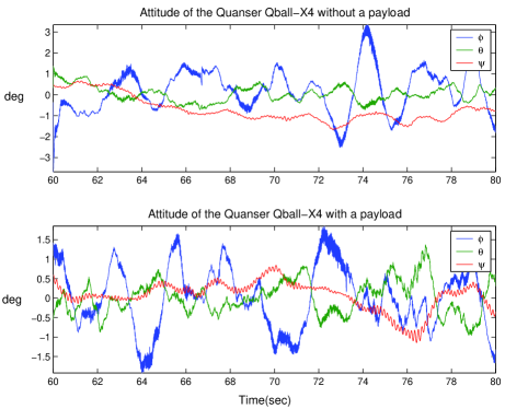
Figure 6: Attitude Stabilization Performance of the ASD Dynamic Inversion Stabilized Controller

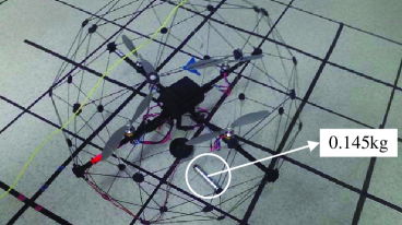
Figure 7: The Quanser Qball-X4 is Attached a 0.145 kg Payload

VI Conclusion

Stabilization for a class of MIMO systems is considered subject to nonparametric time-varying uncertainties with respect to both state and input. This study has three contributions: (i) an ASD dynamic inversion stabilized control, which can solve the stabilization problem for a class of uncertain MIMO systems, (ii) the definition of a new output matrix, which transforms uncertain systems into minimum-phase systems with relative degree one, (iii) a new ASD method, which further transforms the uncertain minimum-phase systems into uncertainty-free systems with one observable lumped disturbance at the output. From the simulations and the experiment, the proposed control scheme has two salient features: less system information required and a simpler design procedure with fewer tuning parameters.

Appendix: Proof of Theorem 2

The following preliminary result is needed.

Lemma 1 [22]. Let $F:$ $\mathbb{R}^{n}\rightarrow\mathbb{R}^{m}$ be continuously differentiable in an open convex set $D\subset\mathbb{R}^{n}$. For any $x,x+p\in D,$ $F\left(x+p\right)$ $-$ $F\left(x\right)$ $=$ $\int_{0}^{1}\left.\frac{\partial F}{\partial z}\right|_{z=x+sp}ds\cdot p.$

Denote $v=h\left(t,u\right)-K^{T}x+\sigma\left(t,x\right).$ Then the system (13) becomes

$$\dot{x}=Ax+Bv$$

and the derivative of $\epsilon\dot{v}$ is calculated to be

$$\epsilon\dot{v} =\frac{\partial h}{\partial u}\epsilon\dot{u}+\epsilon\frac{\partial h}{\partial t}-\epsilon K^{T}\dot{x}+\frac{\partial\sigma}{\partial x}\epsilon\dot{x}+\epsilon\frac{\partial\sigma}{\partial t}$$

$$=\frac{\partial h}{\partial u}\left(-v+\xi\right)+\epsilon\left(-K^{T}+\frac{\partial\sigma}{\partial x}\right)\left(Ax+Bv\right)+\epsilon\frac{\partial h}{\partial t}+\epsilon\frac{\partial\sigma}{\partial t}\text{\ ((\ref{modifiedcontroller3}) is used)}$$

$$=\left[-\frac{\partial h}{\partial u}+\epsilon\left(-K^{T}+\frac{\partial\sigma}{\partial x}\right)B\right]v+\epsilon\frac{\partial h}{\partial t}+\epsilon\frac{\partial\sigma}{\partial t}+\frac{\partial h}{\partial u}\xi+\epsilon\left(-K^{T}+\frac{\partial\sigma}{\partial x}\right)Ax.$$

Consequently, the closed-loop dynamics (29) and (13) are

$$\dot{x} =Ax+bv$$

$$\dot{v} =\left[-\frac{1}{\epsilon}\frac{\partial h}{\partial u}+\left(-K^{T}+\frac{\partial\sigma}{\partial x}\right)B\right]v+\frac{\partial h}{\partial t}+\frac{\partial\sigma}{\partial t}+\frac{1}{\epsilon}\frac{\partial h}{\partial u}\xi+\left(-K^{T}+\frac{\partial\sigma}{\partial x}\right)Ax.$$ (42)

Choose a candidate Lyapunov function as follows:

$$V=x^{T}Px+v^{T}v$$

where $0<P\in\mathbb{R}^{n\times n}\$satisfies (12). Taking the derivative of $V$ along the solution of (42) yields

$$\dot{V} =x^{T}\left(PA+A^{T}P\right)x+2x^{T}PBv+2v^{T}\left[-\frac{1}{\epsilon}\frac{\partial h}{\partial u}+\left(-K^{T}+\frac{\partial\sigma}{\partial x}\right)B\right]v$$

$$\text{ \ \ }+2v^{T}\left(-K^{T}+\frac{\partial\sigma}{\partial x}\right)Ax+2v^{T}\left(\frac{\partial h}{\partial t}+\frac{\partial\sigma}{\partial t}+\frac{1}{\epsilon}\frac{\partial h}{\partial u}\xi\right)$$

$$=x^{T}\left(PA+A^{T}P\right)x+2v^{T}\left(\frac{\partial h}{\partial t}+\frac{\partial\sigma}{\partial t}+\frac{1}{\epsilon}\frac{\partial h}{\partial u}\xi\right)$$

$$\text{ \ \ }-2v^{T}\left[\frac{1}{\epsilon}\frac{\partial h}{\partial u}-\left(-K^{T}+\frac{\partial\sigma}{\partial x}\right)B\right]v+2x^{T}\left[PB-A^{T}\left(-K^{T}+\frac{\partial\sigma}{\partial x}\right)^{T}\right]v.$$

By (12), it follows $x^{T}\left(PA+A^{T}P\right)x\leq-\gamma_{0}\left\|x\right\|^{2},$ where $\gamma_{0}=\lambda_{\min}\left(M\right).$ Then

$$\dot{V} \leq-\gamma_{0}\left\|x\right\|^{2}+2\left\|v\right\|\left(l_{h_{t}}\left\|u\right\|+l_{\sigma_{t}}\left\|x\right\|+d_{\sigma}+\frac{\overline{l}_{h_{u}}}{\epsilon}\left\|\xi\right\|\right)$$

$$\text{ \ \ }-2\left(\frac{1}{\epsilon}\underline{l}_{h_{u}}-\frac{1}{2}\gamma_{1}\right)\left\|v\right\|^{2}+2\gamma_{2}\left\|v\right\|\left\|x\right\|\text{\ \ \ ({Assumptions 2-3} are used)}$$ (43)

Next, the relationship between $\left\|u\right\|$ and $\left\|v\right\|$ needs to be derived to eliminate $\left\|u\right\|$ in (43). By Lemma 1, it follows

$$h\left(t,u\right)=h\left(t,0\right)+\int_{0}^{1}\left.\frac{\partial h}{\partial u}\right|_{x=su}ds\cdot u.$$

Furthermore, since $v=h\left(t,u\right)-K^{T}x+\sigma\left(t,x\right)$, it follows

$$u=\left(\int_{0}^{1}\left.\frac{\partial h}{\partial u}\right|_{x=su}ds\right)^{-1}\left(v+K^{T}x-\sigma\left(t,x\right)-h\left(t,0\right)\right).$$

Further by Assumptions 2-3, the equation above becomes

$$\left\|u\right\| \leq\frac{1}{\underline{l}_{h_{u}}}\left(\left\|v\right\|+\left\|K\right\|\left\|x\right\|+\left\|\sigma\left(t,x\right)\right\|\right)$$

$$\leq\frac{1}{\underline{l}_{h_{u}}}\left(\left\|v\right\|+\left(\left\|K\right\|+k_{\sigma}\right)\left\|x\right\|+\delta_{\sigma}\right).$$

With the above inequality and the further inequality

$$2\left\|v\right\|\left(\frac{l_{h_{t}}}{\underline{l}_{h_{u}}}\delta_{\sigma}+d_{\sigma}+\frac{\overline{l}_{h_{u}}}{\epsilon}\left\|\xi\right\|\right)\leq\frac{1}{\epsilon}\underline{l}_{h_{u}}v^{2}+\frac{\epsilon}{\underline{l}_{h_{u}}}\left(\frac{l_{h_{t}}}{\underline{l}_{h_{u}}}\delta_{\sigma}+d_{\sigma}+\frac{\overline{l}_{h_{u}}}{\epsilon}\left\|\xi\right\|\right)^{2},$$

the inequality (43) becomes

$$\dot{V}\leq-\gamma_{0}\left\|x\right\|^{2}-\left(\frac{1}{\epsilon}\underline{l}_{h_{u}}-\gamma_{1}\right)v^{2}+\frac{\epsilon}{\underline{l}_{h_{u}}}\left(\frac{l_{h_{t}}}{\underline{l}_{h_{u}}}\delta_{\sigma}+d_{\sigma}+\frac{\overline{l}_{h_{u}}}{\epsilon}\left\|\xi\right\|\right)^{2}+2\left(\gamma_{2}+l_{\sigma_{t}}\right)\left\|v\right\|\left\|x\right\|.$$

Since the inequality $2ab\leq a^{2}+b^{2}$ always holds, then

$$2\left(\gamma_{2}+l_{\sigma_{t}}\right)\left\|v\right\|\left\|x\right\|\leq\frac{\gamma_{0}}{2}\left\|x\right\|^{2}+\frac{2}{\gamma_{0}}\left(\gamma_{2}+l_{\sigma_{t}}\right)^{2}v^{2}.$$

Consequently,

$$\dot{V}\leq-\frac{\gamma_{0}}{2}\left\|x\right\|^{2}+\frac{\epsilon}{\underline{l}_{h_{u}}}\left(\frac{l_{h_{t}}}{\underline{l}_{h_{u}}}\delta_{\sigma}+d_{\sigma}+\frac{\overline{l}_{h_{u}}}{\epsilon}\left\|\xi\right\|\right)^{2}-\left[\frac{1}{\epsilon}\underline{l}_{h_{u}}-\gamma_{1}-\frac{2}{\gamma_{0}}\left(\gamma_{2}+l_{\sigma_{t}}\right)^{2}\right]\left\|v\right\|^{2}.$$

Furthermore,

$$\dot{V}\leq-\eta\left(\epsilon\right)V+\frac{\epsilon}{\underline{l}_{h_{u}}}\left(\frac{l_{h_{t}}}{\underline{l}_{h_{u}}}\delta_{\sigma}+d_{\sigma}+\frac{\overline{l}_{h_{u}}}{\epsilon}\left\|\xi\right\|\right)^{2}$$

where $\eta\left(\epsilon\right)=\min(\frac{\gamma_{0}}{2\lambda_{\max}\left(P\right)},\frac{1}{\epsilon}\underline{l}_{h_{u}}-\gamma_{1}-\frac{2}{\gamma_{0}}\left(\gamma_{2}+l_{\sigma_{t}}\right)^{2}).$ If (30) is satisfied, then $\eta\left(\epsilon\right)>0.$ So, $V\left(t\right)\rightarrow\mathcal{B}\left(\frac{1}{\eta\left(\epsilon\right)}\frac{\epsilon}{\underline{l}_{h_{u}}}\left(\frac{l_{h_{t}}}{\underline{l}_{h_{u}}}\delta_{\sigma}+d_{\sigma}+\frac{\overline{l}_{h_{u}}}{\epsilon}\left\|\xi\right\|\right)^{2}\right)$ as $t\rightarrow\infty$, namely

$$\left\|x\left(t\right)\right\|\rightarrow\mathcal{B}\left(\sqrt{\frac{\epsilon}{\lambda_{\min}\left(P\right)\eta\left(\epsilon\right)\underline{l}_{h_{u}}}}\left(\frac{l_{h_{t}}}{\underline{l}_{h_{u}}}\delta_{\sigma}+d_{\sigma}+\frac{\overline{l}_{h_{u}}}{\epsilon}\left\|\xi\right\|\right)\right)$$

as$\ t\rightarrow\infty,$ where $\mathcal{B}\left(\delta\right)\triangleq\left\{\xi\in\mathbb{R}\left|\left\|\xi\right\|\leq\delta\right.\right\},$ $\delta>0.$ The notation $z\left(t\right)\rightarrow\mathcal{B}\left(\delta\right)$ means $\underset{y\in\mathcal{B}\left(\delta\right)}{\min}$ $\left|z\left(t\right)-y\right|\rightarrow 0$ as $t\rightarrow\infty.$ Since $\xi\rightarrow 0$ as $t\rightarrow\infty,$ $\left\|x\left(t\right)\right\|\rightarrow\mathcal{B}\left(\sqrt{\frac{\epsilon}{\lambda_{\min}\left(P\right)\eta\left(\epsilon\right)\underline{l}_{h_{u}}}}\left(\frac{l_{h_{t}}}{\underline{l}_{h_{u}}}\delta_{\sigma}+d_{\sigma}\right)\right).$ Furthermore, if $l_{h_{t}}\delta_{\sigma}\left(t\right)\rightarrow 0$ and$\ d_{\sigma}\left(t\right)\rightarrow 0,$ then the state $x\left(t\right)\rightarrow 0$ as $t\rightarrow\infty.$

References

- [1] Apkarian, P., and Biannic, J.-M., and Gahinet, P., “Self-scheduled H-infinity Control of Missile via Linear Matrix Inequalities,” Journal of Guidance, Control, and Dynamics, Vol. 18, No. 3, 1995, pp. 532–538. doi: 10.2514/3.21419.
- [2] Malloy, D., Chang, B.C., “Stabilizing Controller Design for Linear Parameter-Varying Systems Using Parameter Feedback,” Journal of Guidance, Control, and Dynamics, Vol. 21, No. 6, 1998, pp. 891–898. doi: 10.2514/2.4322.
- [3] Young, A., Cao, C., Patel, V., Hovakimyan, N., Lavretsky E., “Adaptive Control Design Methodology for Nonlinearin-Control Systems in Aircraft Applications,” Journal of Guidance, Control, and Dynamics, Vol. 30, No. 6, 2007, pp. 1770–1786. doi: 10.2514/2.4600. doi: 10.2514/1.27969.
- [4] Hovakimyan, N., Lavretsky, E., Cao, C., “Dynamic Inversion for Multivariable Non-Affine-in-Control Systems via Time-Scale Separation,” International Journal of Control, Vol. 81, No. 12, 2008, pp. 1960–1967. doi: 10.1080/00207170801961295.
- [5] Lavretsky, E., Hovakimyan, N., “Adaptive Dynamic Inversion for Nonaffine-in-Control Uncertain Systems via Time-Scale Separation. Part II,” Journal of Dynamical Systems and Control, Vol. 14, No. 1, 2008, pp. 33-41. doi: 10.1007/s10883-007-9033-5.
- [6] Cao, C., and Hovakimyan, N., “Stability Margins of Adaptive Control Architecture,” IEEE Transaction on Automatic Control, Vol. 55, No. 2, 2010, pp. 480–487. doi: 10.1109/TAC.2009.2037384.
- [7] Chaturvedi, N.A., Sanyal, A.K., Chellappa, M., Valk, J.L., McClamroch., N.H., and Bernstein, D.S., “Adaptive Tracking of Angular Velocity for a Planar Rigid Body with Unknown Models for Inertia and Input Nonlinearity,” IEEE Transactions on Control Systems Technology, Vol. 14, No. 4, 2006, pp. 613–627. doi: 10.1109/TCST.2006.876628.
- [8] MacKunis, W., Patre, P.M., Kaiser, M.K., and Dixon, W.E., “Asymptotic Tracking for Aircraft via Robust and Adaptive Dynamic Inversion Methods,” IEEE Transactions on Control Systems Technology, Vol. 18, No. 6, 2010, pp. 1448–1456. doi: 10.1109/TCST.2009.2039572.
- [9] Landau, I.D., Lozano, R., M’Saad, M., Karimi, A., “Adaptive Control: Algorithms, Analysis and Applications,” Springer, London, 2011, pp. 111-118.
- [10] Singhal, C., Tao, G., and Burkholder, J.O., “Neural Network-Based Compensation of Synthetic Jet Actuator Nonlinearities for Aircraft Flight Control,” AIAA Paper 2009-6177, Aug. 2009. doi: 10.2514/6.2009-6177.
- [11] Chen, M., Ge, S.S., and How B.V.E., “Robust Adaptive Neural Network Control for a Class of Uncertain MIMO Nonlinear Systems with Input Nonlinearities,” IEEE Transactions on Neural Networks, Vol. 21, No. 5, 2010, pp. 796–812. doi: 10.1109/TNN.2010.2042611.
- [12] Zhang, T., and Guay, M., “Adaptive Control for a Class of Second-Order Nonlinear Systems with Unknown Input Nonlinearities,” IEEE Transactions on Systems, Man and Cybernetics—Part B: Cybernetics, Vol. 33, No. 1, 2003, pp. 143–149. doi: 10.1109/TSMCB.2003.808187.
- [13] Hsu, K.-C., “Sliding Mode Controllers for Uncertain Systems with Input Nonlinearities,” Journal of Guidance, Control, and Dynamics, Vol. 21, No. 4, 1998, pp. 666–669. doi: 10.2514/2.4289.
- [14] Shen, Y., Liu, C., and Hu, H., “Output Feedback Variable Structure Control for Uncertain Systems with Input Nonlinearities,” Journal of Guidance, Control, and Dynamics, Vol. 23, No.4, 1999, pp. 762–764. doi: 10.2514/2.4600.
- [15] Quan, Q., and Cai, K.-Y., “Additive Decomposition and Its Applications to Internal-Model-Based Tracking,” Joint 48th IEEE Conference on Decision and Control and 28th Chinese Control Conference, IEEE Publications, Shanghai, China, 2009, pp. 817–822. doi: 10.1109/CDC.2009.5400007.
- [16] Teo, J., How, J.P., Lavretsky E., “Proportional-Integral Controllers for Minimum-Phase Nonaffine-in-Control Systems,” IEEE Transactions on Automatic Control, Vol. 55, No. 6, 2010, pp. 1477–1483. doi: 10.1109/TAC.2010.2045693.
- [17] Quan, Q., Cai, K.-Y., “Additive-State-Decomposition-Based Tracking Control for TORA Benchmark,” Journal of Sound and Vibration, Vol. 332, No. 20, 2013, pp. 4829–4841. doi: 10.1016/j.jsv.2013.04.033.
- [18] Quan, Q., Cai K.-Y., Lin, H., “Additive-State-Decomposition-Based Tracking Control Framework for a Class of Nonminimum Phase Systems with Measurable Nonlinearities and Unknown Disturbances,” International Journal of Robust and Nonlinear Control, online. doi: 10.1002/rnc.3079.
- [19] Quan, Q., Lin, H., Cai K.-Y. “Output Feedback Tracking Control by Additive State Decomposition for a Class of Uncertain Systems,” International Journal of Systems Science, online. doi: 10.1080/00207721.2012.757379.
- [20] Quan Q., Cai K.-Y. “Additive-Output-Decomposition-Based Dynamic Inversion Tracking Control for a Class of Uncertain Linear Time-Invariant Systems,” The 51st IEEE Conference on Decision and Control, IEEE Publications, Maui, Hawaii, USA, 2012, pp. 2866-2871. doi: 10.1109/CDC.2012.6427111.
- [21] Stevens, B., and Lewis, F., “Aircraft Control and Simulation,” Wiley, New York, 1992, pp. 584-592.
- [22] Dennis, J.E., and Schnabel R.B, “Numerical Methods for Unconstrained Optimization and Nonlinear Equations,” SIAM, 1987, p.74.