Effects of Resistivity on Magnetized Core-Collapse Supernovae

Abstract

We studied roles of a turbulent resistivity in the core-collapse of a strongly magnetized massive star, carrying out 2D-resistive-MHD simulations. The three cases with different initial strengths of magnetic field and rotation are investigated; 1. strongly magnetized rotating core; 2. moderately magnetized rotating core; 3. very strongly magnetized non-rotating core. In each case, both an ideal-MHD model and resistive-MHD models are computed. As a result of computations, each model shows a matter eruption helped by a magnetic acceleration (and also by a centrifugal acceleration in the rotating cases). We found that a resistivity attenuates the explosion in case 1 and 2, while it enhances the explosion in case 3. We also found that in the rotating cases, main mechanisms for the amplification of a magnetic field in the post-bounce phase are an outward advection of magnetic field and a winding of poloidal magnetic field-lines by differential rotation, which are somewhat dampened down with the presence of a resistivity. Although the magnetorotational instability seems to occur in the rotating models, it will play only a minor role in a magnetic field amplification. Another impact of resistivity is that on the aspect ratio. In the rotating cases, a large aspect ratio of the ejected matters, $>2.5$, attained in a ideal-MHD model is reduced to some extent in a resistive model. These results indicate that a resistivity possibly plays an important role in the dynamics of strongly magnetized supernovae.

1. Introduction

Studies on magnetized core-collapse supernovae (CCSNe) has gathered stream for past several years. Numerical simulations so far have shown that the presence of strong magnetic field together with rapid rotation results in a vigorous matter eruption accompanied by bipolar jets with an explosion energy of $\sim 10^{51}$ erg (magnetorotational explosion: LeBlanc & Wilson, 1970; Symbalisty, 1984; Yamada & Sawai, 2004). One of the main driving forces is a toroidal magnetic pressure amplified by differential rotation that becomes intense after the collapse in the vicinity of proto-neutron star surface. This mechanism requires a magnetic field strength of $\gtrsim 10^{15}$ G after collapse, which is comparable to an inferred surface magnetic field of magnetar candidates, soft-gamma repeaters (SGR) and anomalous X-ray pulsars (AXP). Magnetically-driven explosions may be related to such supernovae that produce magnetars.

Most numerical simulations of magnetized core-collapse so far have been done in the regime of ideal magnetohydrodynamics (MHD) (e.g. Kotake et al., 2004; Sawai et al., 2005; Moiseenko et al., 2006; Burrows et al., 2007; Sawai et al., 2008; Takiwaki et al., 2009; Obergaulinger & Janka, 2011; Endeve et al., 2012). The only exception is the numerical study by Guilet et al. (2011), in which a resistivity is introduced to 1D-MHD simulations investigating the dynamics of an Alfvén surface in the context of core-collapse supernovae. Although a numerical computation with a finite differential scheme inevitably involves numerical diffusion, effects of electric resistivity on the dynamics have not been investigated systematically. The reason why a resistivity has been neglected is that it would be infinitesimally small assuming that the source is the Coulomb scattering (Spitzer resistivity; Spitzer (1956)). The magnetic Reynolds number, the ratio of the resistive timescale to dynamical timescale, estimated with a typical parameters of proto-neutron star surface is

$$R_{\textrm{m}} \sim 8\times 10^{15}\left(\displaystyle\frac{Z}{26}\right)^{-1}\left(\displaystyle\frac{T}{5\times 10^{10}\textrm{K}}\right)^{3/2}$$

$$\times\left(\displaystyle\frac{L}{4\times 10^{5}\textrm{cm}}\right)\left(\displaystyle\frac{v}{2\times 10^{8}\textrm{cm s}^{-1}}\right),$$

where $Z$, $T$, $L$, and $v$ are, respectively, an atomic charge number, temperature, scale length of magnetic field, and flow velocity. Since the magnetic Reynolds number is quite larger than unity, a resistivity apparently seems not important for the dynamics.

However, it is uncertain whether the Coulomb scattering is the unique origin of resistivity in a supernova core, and there may exist other sources that give rise to a dynamically important value of resistivity. One of such candidates is a turbulence. In the collapsed core of a massive star, a convection, which occurs due to negative gradient of entropy and/or electron fraction, may play a key role to produce a turbulent state and a turbulent resistivity (and viscosity) along with that. Thompson et al. (2005) roughly estimated the amplitude of a turbulent viscosity arising from convective motions in a supernova core by the product of the correlation length and convective velocity, $\xi_{\rm{con}}\sim lv_{\rm{con}}/3$. They found that $\xi_{\rm{con}}$ is around $10^{13}-10^{14}$ cm² s^-1. Insofar as this level of estimation, the amplitude of a turbulent resistivity may be evaluated by the same formula and may be comparable to a turbulent viscosity, since magnetic field would have a similar timescale and length-scale with those of velocity in the present situation. Yoshizawa (1990) showed in the frame work of so-called two-scale direct-interaction approximation that the magnitude of a turbulent viscosity and turbulent resistivity are same order, albeit in the context of an incompressible MHD turbulence. With the above amplitude of the turbulent resistivity, the magnetic Reynolds number becomes $\sim 1-10$ around the surface of a proto-neutron star, and then a resistivity is possibly important for the dynamics.

In this paper, we investigate how a (turbulent) resistivity alters the dynamics of a magnetized core-collapse, paying particular attention to the explosion energy, the magnetic field amplification, and the aspect ratio of ejected matters. To this end we carried out axisymmetric 2D-resistive-MHD simulations of the core-collapse of a massive star, assuming a strong magnetic field and a large resistivity. A constant resistivity of $10^{13}$ and $10^{14}$ cm² s^-1 are taken according to the above discussion. Both rapidly rotating and non-rotating cores are studied. In the computations, we omitted any treatments of neutrinos, and adopted a nuclear equation of state (EOS) produced by Shen et al. (1998a, b).

Before proceeding to the next section, we go into a little more detail on a convection as a source of a turbulent resistivity, and also mention our position in choosing the initial strength of a magnetic field and a rotation.

In a collapsed stellar core, there are mainly two convectively unstable regions (see e.g. Herant et al. (1994)). One is a region behind the shock surface, where a negative entropy gradient is created as the shock surface propagates with its amplitude decreasing, and is maintained by a neutrino heating. The other is a region around the proto-neutron star surface, where a negative gradient of lepton fraction is created because a neutrino is easier to escape from the core for a lager radius. Since we do not deal with neutrinos, convections related to them are not captured in the computations. Only convection that seems to appear in our computation is one due to the shock propagation with a decreasing amplitude. Nevertheless, we assume all of the above convections as sources of a turbulent resistivity adopted in this study, since they will occur in the nature. What we have done here is to effectively introduce an impact of these convections to the simulations. In so doing, it does not seem quite important whether they are properly captured in the simulations. Note that we do not consider that the standing accretion shock instability (SASI), which do not present in our computations, is one of the origins of a turbulent resistivity, because all of our models explode before this instability can develop (several 100 ms after bounce), owing to strong magnetic fields initially assumed.

Although a turbulent resistivity will appear only around the convectively unstable regions, in our computations a constant resistivity is assumed everywhere except in the vicinity of the center (see § 3). Also, we should note that the estimation made by Thompson et al. (2005) is very uncertain. Moreover, strong magnetic fields initially assumed may decrease the strength of a turbulent resistivity. Therefore, the strengths of an adopted turbulent resistivity are perhaps too large to be realistic. However, at present a probable value of a turbulent resistivity in a collapsed-stellar core is very unclear. Under such a circumstance, it is meaningful to parametrically study its effect with some possible values, and to grasp dynamical trends. We consider that the adopted strengths of a turbulent resistivity may be maximum possible values.

A strongly magnetized core prior to collapse assumed in the present study is based on so-called ”fossil-field hypothesis,” which supposes that the progenitor of a magnetar already has a magnetar-class magnetic flux during the main sequence stage. Assuming this hypothesis, Ferrario & Wickramasinghe (2006) have done population synthesis calculations from main sequence stars to neutron stars, to fit observational data of radio pulsars. Their calculation produces consistent number of magnetars with those observed in the Galaxy, where both the age and rotational period of magnetars are taken into account. The fossil field hypothesis is also supported by observations. There are several O-type stars whose surface magnetic flux is inferred to be a magnetar-class; e.g. HD148937 (Wade et al., 2012) and HD19612 (Donati et al., 2006). Aurière et al. (2010) measured surface magnetic fields of Betelgeuse, a red supergiant star, to be $\sim 1$ G, which indicates a magnetar-class magnetic flux. Note, however, that the origin of a strong magnetic fields in magnetars is still controversial. Alternatively, they may be produced during the core-collapse by a dynamo mechanism (Thompson & Duncan, 2003).

Heger et al. (2005) found that the so-called Tayler-Spruit dynamo (Spruit, 2002) drastically slows down the rotation of a star especially during an early phase of red super giant, where an angular momentum of the rapidly rotating helium core is transported into the slowly rotating hydrogen envelope. According to their computation, an inferred rotational period of a pulser is $\sim 10$ ms for a $15~{}M_{\odot}$ progenitor, in which the available rotational energy is insufficient for the explosion. On the other hand, Woosley & Heger (2006) carried out stellar evolution computations of inherently rapid rotators, and showed that the rotation of a pre-supernova core could be fast. Due to the fast rotation, matters are almost completely mixed, and instead of forming a red supergiant it becomes a compact helium core star, where a magnetic torque works less efficiently. One of their $16M_{\odot}$ magnetic star models with the solar metalicity results in the expected pulsar rotation period of $2.3$ ms, sufficient for a magnetorotational explosion. Note that the both works involve uncertainties about such as mass loss rate and multi-dimensional effects. At present, it is unclear either of slow or fast rotation is appropriate for the progenitor of a magnetar. Hence, in this study both rapidly rotating models and non-rotating models are investigated, where the latter, in effect, corresponds to a slow rotation case.

The rest of this paper is organized as follows. We describe the governing equations and essentials of our resistive-MHD code in § 2, and computational setups in § 3. The results are presented in § 4. Discussion and conclusion are given in § 5.

2. Governing Equations and Numerical Schemes

In order to follow the dynamics of magnetized core-collapses with resistivity, the resistive-MHD equations below are solved:

$$\frac{\partial\rho}{\partial t}+\nabla\cdot(\rho\mbox{\boldmath$v$})=0,$$ (1)

$$\frac{\partial}{\partial t}(\rho\mbox{\boldmath$v$})+\nabla\cdot\left(\rho\mbox{\boldmath$v$}\mbox{\boldmath$v$}-\frac{\mbox{\boldmath$B$}\mbox{\boldmath$B$}}{4\pi}\right)$$

$$\hskip 12.0pt=-\nabla\left(p+\frac{B^{2}}{8\pi}\right)-\rho\nabla\Phi,$$ (2)

$$\frac{\partial}{\partial t}\left(e+\frac{\rho v^{2}}{2}+\frac{B^{2}}{8\pi}\right)$$

$$\hskip 12.0pt+\nabla\cdot\left[\left(e+p+\frac{\rho v^{2}}{2}+\frac{B^{2}}{4\pi}\right)\mbox{\boldmath$v$}\right.$$

$$\hskip 48.0pt\left.-\frac{(\mbox{\boldmath$v$}\cdot\mbox{\boldmath$B$})\mbox{\boldmath$B$}}{4\pi}+\frac{\eta}{c}\mbox{\boldmath$j$}\times\mbox{\boldmath$B$}\right]$$

$$\hskip 48.0pt=-\rho(\nabla\Phi)\cdot\mbox{\boldmath$v$},$$ (3)

$$\frac{\partial\mbox{\boldmath$B$}}{\partial t}+c\nabla\times\mbox{\boldmath$E$}=0,$$ (4)

$$\mbox{\boldmath$E$}=-\frac{1}{c}\mbox{\boldmath$v$}\times\mbox{\boldmath$B$}+\frac{4\pi\eta}{c^{2}}\mbox{\boldmath$j$},$$ (5)

$$\mbox{\boldmath$j$}=\frac{c}{4\pi}\nabla\times\mbox{\boldmath$B$},$$ (6)

in which notations of the physical variables follow custom.

To solve above equations we have developed 2D-resistive-MHD code, ”Yamazakura.” This is a time explicit, Eulerian code based on the high resolution central scheme formulated by Kurganov & Tadmor (2000) (Here after KT scheme). Below we briefly describe the features of Yamazakura. For sake of simplicity, we deal in the case where the equations are written in Cartesian coordinate with plane symmetry in $z$-direction.

The KT scheme adopts a finite volume method to solve conservation equations. Although the induction equations (4) apparently seem written in non-conservation forms, they are rewritten into conservation forms (Ziegler, 2004);

$$\frac{\partial B^{x}}{\partial t}+c\nabla\cdot\left(\begin{array}[]{cc}\hphantom{-}0\hphantom{{}^{-}},&\hphantom{-}E^{z}\end{array}\right)=0,$$ (8)

$$\frac{\partial B^{y}}{\partial t}+c\nabla\cdot\left(\begin{array}[]{cc}-E^{z},&\hphantom{-}0\hphantom{{}^{-}}\end{array}\right)=0,$$ (10)

$$\frac{\partial B^{z}}{\partial t}+c\nabla\cdot\left(\begin{array}[]{cc}\hphantom{-}E^{y},&-E^{x}\end{array}\right)=0.$$ (12)

Then evolutionary Eqs. (1)$-$(3) and (10) are all written in conservation forms with source terms;

$$\frac{\partial\mbox{\boldmath$u$}}{\partial t}+\nabla\cdot\left(\begin{array}[]{ccc}\mbox{{\boldmath$f$}}^{x}\left(\mbox{{\boldmath$u$}}\right),&\mbox{{\boldmath$f$}}^{y}\left(\mbox{{\boldmath$u$}}\right)&\end{array}\right)$$ (14)

$$\hskip 16.79993pt+\nabla\cdot\left(\begin{array}[]{ccc}\mbox{{\boldmath$g$}}^{x}\left(\mbox{{\boldmath$u$}},\mbox{{\boldmath$u$}}_{,x},\mbox{{\boldmath$u$}}_{,y}\right),&\mbox{{\boldmath$g$}}^{y}\left(\mbox{{\boldmath$u$}},\mbox{{\boldmath$u$}}_{,x},\mbox{{\boldmath$u$}}_{,y}\right)&\end{array}\right)=\mbox{{\boldmath$s$}}(\mbox{{\boldmath$u$}}),$$ (16)

where a expression such as $\nabla\cdot(\mbox{{\boldmath$f$}}^{x},\mbox{{\boldmath$f$}}^{y})$ means $\partial\mbox{{\boldmath$f$}}^{x}/\partial x+\partial\mbox{{\boldmath$f$}}^{y}/\partial y$. The vectors in Eq. (14), each of which has eight components, are given as follows:

$$u = \left(\begin{array}[]{c}\rho\\ \rho v^{x}\\ \rho v^{y}\\ \rho v^{z}\\ e+\rho v^{2}/2+B^{2}/8\pi\\ B^{x}\\ B^{y}\\ B^{z}\end{array}\right),$$ (25)

$$\mbox{\boldmath$f$}^{x} = \left(\begin{array}[]{c}\rho v^{x}\\ \rho v^{x}v^{x}-B^{x}B^{x}/4\pi+p+B^{2}/8\pi\\ \rho v^{x}v^{y}-B^{x}B^{y}/4\pi\\ \rho v^{x}v^{z}-B^{x}B^{z}/4\pi\\ (e+p+\rho v^{2}/2+B^{2}/4\pi)v^{x}-(\mbox{\boldmath$v$}\cdot\mbox{\boldmath$B$})B^{x}/4\pi\\ 0\\ v^{x}B^{y}-v^{y}B^{x}\\ -v^{z}B^{x}+v^{x}B^{z}\end{array}\right),$$ (34)

$$\mbox{\boldmath$f$}^{y} = \left(\begin{array}[]{c}\rho v^{y}\\ \rho v^{y}v^{x}-B^{y}B^{x}/4\pi\\ \rho v^{y}v^{y}-B^{y}B^{y}/4\pi+p+B^{2}/8\pi\\ \rho v^{y}v^{z}-B^{y}B^{z}/4\pi\\ (e+p+\rho v^{2}/2+B^{2}/4\pi)v^{y}-(\mbox{\boldmath$v$}\cdot\mbox{\boldmath$B$})B^{y}/4\pi\\ -v^{x}B^{y}+v^{y}B^{x}\\ 0\\ v^{y}B^{z}-v^{z}B^{y}\end{array}\right),$$ (43)

$$\mbox{\boldmath$g$}^{x} = \left(\begin{array}[]{c}0\\ 0\\ 0\\ 0\\ \eta(j^{y}B^{z}-j^{z}B^{y})/c\\ 0\\ -4\pi\eta j_{z}/c\\ 4\pi\eta j_{y}/c\end{array}\right),$$ (52)

$$\mbox{\boldmath$g$}^{y} = \left(\begin{array}[]{c}0\\ 0\\ 0\\ 0\\ \eta(j^{z}B^{x}-j^{x}B^{z})/c\\ 4\pi\eta j_{z}/c\\ 0\\ -4\pi\eta j_{x}/c\end{array}\right),$$ (61)

$$s = \left(\begin{array}[]{c}0\\ -\rho\partial\Phi/\partial x\\ -\rho\partial\Phi/\partial y\\ -\rho\partial\Phi/\partial z\\ -\rho(\nabla\Phi)\cdot\mbox{\boldmath$v$}\\ 0\\ 0\\ 0\end{array}\right).$$

The KT scheme is written as follows:

$$\frac{d\mbox{{\boldmath$u$}}_{i,j}(t)}{dt} = -\frac{\mbox{{\boldmath$F$}}^{x}_{i+1/2,j}(t)-\mbox{{\boldmath$F$}}^{x}_{i-1/2,j}(t)}{\Delta x_{i}}$$ (70)

$$-\frac{\mbox{{\boldmath$F$}}^{y}_{i,j+1/2}(t)-\mbox{{\boldmath$F$}}^{y}_{i,j-1/2}(t)}{\Delta y_{j}}$$

$$-\frac{\mbox{{\boldmath$G$}}^{x}_{i+1/2,j}(t)-\mbox{{\boldmath$G$}}^{y}_{i-1/2,j}(t)}{\Delta x_{i}}$$

$$-\frac{\mbox{{\boldmath$G$}}^{y}_{i,j+1/2}(t)-\mbox{{\boldmath$G$}}^{y}_{i,j-1/2}(t)}{\Delta y_{j}}+\mbox{{\boldmath$s$}}_{i,j}(t),$$

where $\Delta x_{i}=x_{i+1/2}-x_{i-1/2}$, $\Delta y_{j}=y_{j+1/2}-y_{j-1/2}$, and an integer and half-integer subscript respectively means that a variable is evaluated at the numerical cell center and interface. The numerical fluxes $F$ and $G$ are for the non-resistive terms and resistive terms, respectively. The numerical fluxes of non-resistive terms are given by

$$\mbox{{\boldmath$F$}}^{x}_{i+1/2,j}(t) \equiv \frac{\mbox{{\boldmath$f$}}^{x}\left(\mbox{{\boldmath$u$}}^{+}_{i+1/2,j}(t)\right)+\mbox{{\boldmath$f$}}^{x}\left(\mbox{{\boldmath$u$}}^{-}_{i+1/2,j}(t)\right)}{2}$$

$$-\frac{a_{i+1/2,j}(t)}{2}\left[\mbox{{\boldmath$u$}}^{+}_{i+1/2,j}(t)-\mbox{{\boldmath$u$}}^{-}_{i+1/2,j}(y)\right],$$

$$\mbox{{\boldmath$F$}}^{y}_{i,j+1/2}(t) \equiv \frac{\mbox{{\boldmath$f$}}^{y}\left(\mbox{{\boldmath$u$}}^{+}_{i,j+1/2}(t)\right)+\mbox{{\boldmath$f$}}^{y}\left(\mbox{{\boldmath$u$}}^{-}_{i,j+1/2}(t)\right)}{2}$$

$$-\frac{a_{i,j+1/2}(t)}{2}\left[\mbox{{\boldmath$u$}}^{+}_{i,j+1/2}(t)-\mbox{{\boldmath$u$}}^{-}_{i,j+1/2}(t)\right].$$

The numerical fluxes of the resistive terms, $\mbox{{\boldmath$G$}}^{x}$ and $\mbox{{\boldmath$G$}}^{y}$, are to appear later.

In the original KT scheme, the interface values in Eq. (LABEL:eq.kt.numfluxf), which have a superscript ”$+$” or ”$-$”, are evaluated by a interpolation of conservative variables $u$:

$$\mbox{{\boldmath$u$}}^{+}_{i+1/2,j}(t) = \mbox{{\boldmath$u$}}_{i+1,j}(t)-\frac{\Delta x_{i+1}}{2}(\mbox{{\boldmath$u$}}_{,x})_{i+1,j}(t),$$

$$\mbox{{\boldmath$u$}}^{-}_{i+1/2,j}(t) = \mbox{{\boldmath$u$}}_{i,j}(t)_{\hphantom{+1}}+\frac{\Delta x_{i\hphantom{+1}}}{2}(\mbox{{\boldmath$u$}}_{,x})_{i,j}(t),$$

$$\mbox{{\boldmath$u$}}^{+}_{i,j+1/2}(t) = \mbox{{\boldmath$u$}}_{i,j+1}(t)-\frac{\Delta y_{j+1}}{2}(\mbox{{\boldmath$u$}}_{,y})_{i,j+1}(t),$$

$$\mbox{{\boldmath$u$}}^{-}_{i,j+1/2}(t) = \mbox{{\boldmath$u$}}_{i,j}(t)_{\hphantom{+1}}+\frac{\Delta y_{j\hphantom{+1}}}{2}(\mbox{{\boldmath$u$}}_{,y})_{i,j}(t).$$ (72)

Alternatively, we may be able to use interpolated interface values of the primitive variables $\mbox{{\boldmath$q$}}=(\rho,v_{x},v_{y},v_{z},e,B_{x},B_{y},B_{z})$,

$$\mbox{{\boldmath$q$}}^{+}_{i+1/2,j}(t) = \mbox{{\boldmath$q$}}_{i+1,j}(t)-\frac{\Delta x_{i+1}}{2}(\mbox{{\boldmath$q$}}_{,x})_{i+1,j}(t),$$

$$\mbox{{\boldmath$q$}}^{-}_{i+1/2,j}(t) = \mbox{{\boldmath$q$}}_{i,j}(t)_{\hphantom{+1}}+\frac{\Delta x_{i\hphantom{+1}}}{2}(\mbox{{\boldmath$q$}}_{,x})_{i,j}(t),$$

$$\mbox{{\boldmath$q$}}^{+}_{i,j+1/2}(t) = \mbox{{\boldmath$q$}}_{i,j+1}(t)-\frac{\Delta y_{j+1}}{2}(\mbox{{\boldmath$q$}}_{,y})_{i,j+1}(t),$$

$$\mbox{{\boldmath$q$}}^{-}_{i,j+1/2}(t) = \mbox{{\boldmath$q$}}_{i,j}(t)_{\hphantom{+1}}+\frac{\Delta y_{j\hphantom{+1}}}{2}(\mbox{{\boldmath$q$}}_{,y})_{i,j}(t),$$ (73)

to evaluate the interface values of the conservative variables in Eqs. (LABEL:eq.kt.numfluxf), e.g.,

$$\mbox{{\boldmath$u$}}^{+}_{i+1/2,j}(t) = \mbox{{\boldmath$u$}}\left(\mbox{{\boldmath$q$}}^{+}_{i+1/2,j}(t)\right).$$

In Yamazakura, we adopt the latter prescription. For the calculation of the numerical derivatives, $\mbox{{\boldmath$q$}}_{,x}$ and $\mbox{{\boldmath$q$}}_{,y}$, in Eqs. (73), we employ a minmod-like limiter suggested by Kurganov & Tadmor (2000). Note that the interpolations (73) are only used for the hydrodynamical quantities and the $z$-component of magnetic field, which are placed at the center of a numerical cell. Those for the $x$-component and $y$-component of magnetic field are given later.

In Eqs. (LABEL:eq.kt.numfluxf), $a_{i+1/2,j}(t)$ and $a_{i,j+1/2}(t)$ are the maximum characteristic speeds, i.e. the sum of the fluid velocity and fast magnetosonic speed, which we evaluate using the interpolated primitive variables in Eqs. (73):

$$a_{i+1/2,j}(t) = \max\left\{a\left(\mbox{{\boldmath$q$}}^{+}_{i+1/2,j}(t)\right),a\left(\mbox{{\boldmath$q$}}^{-}_{i+1/2,j}(t)\right)\right\},$$

$$a_{i-1/2,j}(t) = \max\left\{a\left(\mbox{{\boldmath$q$}}^{+}_{i-1/2,j}(t)\right),a\left(\mbox{{\boldmath$q$}}^{-}_{i-1/2,j}(t)\right)\right\}.$$

In KT scheme, we only need to know these maximum characteristic speeds instead of carrying out a complicated characteristic decomposition for wave propagations.

The original KT scheme is formulated for uniform spatial cells. We have followed the procedure to deduce the KT scheme described in Kurganov & Tadmor (2000) with non-uniform cells, and found that the final semi-discrete form (70)$-$(72) is unchanged, except that the subscripts to $\Delta x$ and $\Delta y$ appear.

In order to obtain the time evolution of conservative variables $\mbox{{\boldmath$u$}}_{i,j}(t)$, the semi-discrete equation (70) is time integrated utilizing a third order Runge-Kutta method according to Kurganov & Tadmor (2000). With this and the spatial interpolations in Eqs. (72), the original KT scheme is a third order in time and second order in space. In Appendix (”Linear Wave Propagation”), it is shown that Yamazakura performs, approximately, at least second order in time and second order in space, even though we adopt a non-uniform cell distribution and the spatial interpolations of the primitive variables (Eqs. (73)).

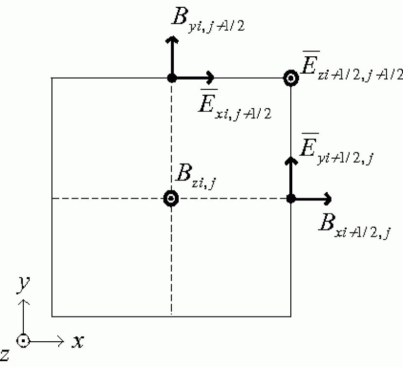
Figure 1.— Positional relation of magnetic field vectors and numerical fluxes (or electric field vectors), $\bar{E}$.

In solving MHD equations, it is necessary to satisfy the divergence-free constraint of magnetic field. To accomplish this, we apply a constraint transport (CT) method to KT scheme based on Ziegler (2004), extending it into resistive-MHD case. In a 3D-CT method, a magnetic field vector is placed at the center of a cubic cell interface while a numerical flux (or an electric field vector) is at a cell edge so that $\nabla\cdot\mbox{{\boldmath$B$}}$ does not evolve (Evans & Hawley, 1988). The positional relation between them in 2D case are shown in Fig 1. Due to this placement, the semi-discrete equations and the numerical fluxes of the induction equations should be different from Eqs. (70) and (LABEL:eq.kt.numfluxf). With numerical fluxes, $\bar{E}$ = $\mbox{{\boldmath$\bar{F}$}}+\mbox{{\boldmath$\bar{G}$}}$, the semi-discrete form of the induction equations are written as

$$\frac{d}{dt}B^{x}_{i+1/2,j} = -\frac{\bar{E}^{z}_{i+1/2,j+1/2}-\bar{E}^{z}_{i+1/2,j-1/2}}{\Delta y_{j}},$$

$$\frac{d}{dt}B^{y}_{i,j+1/2} = \hphantom{-}\frac{\bar{E}^{z}_{i+1/2,j+1/2}-\bar{E}^{z}_{i-1/2,j+1/2}}{\Delta x_{i}},$$ (75)

$$\frac{d}{dt}B^{z}_{i,j}\hphantom{{}_{+1/2}} = -\frac{\bar{E}^{y}_{i+1/2,j}-\bar{E}^{y}_{i-1/2,j}}{\Delta x_{i}}+\frac{\bar{E}^{x}_{i,j+1/2}-\bar{E}^{x}_{i,j-1/2}}{\Delta y_{j}}.$$

The numerical fluxes of the non-resistive terms are

$$\bar{F}^{x}_{i,j+1/2\hphantom{+1/2}} = -F^{y(8)}_{i,j+1/2}$$

$$\bar{F}^{y}_{i+1/2,j\hphantom{+1/2}} = \hphantom{-}F^{x(8)}_{i+1/2,j}$$ (76)

$$\bar{F}^{z}_{i+1/2,j+1/2} = \frac{1}{4}\left(-F^{x(7)}_{i+1/2,j}-F^{x(7)}_{i+1/2,j+1}\right.$$

$$\hskip 14.39996pt\left.+F^{y(6)}_{i,j+1/2}+F^{y(6)}_{i+1,j+1/2}\right),$$

where $F^{\{x,y\}(m)}$ denotes the m-th component of the vector $\mbox{{\boldmath$F$}}^{\{x,y\}}$. The interpolations for the $x$-component and $y$-component of a magnetic field along the x-direction are given by

$$B^{x+}_{i+1/2,j} = B^{x}_{i+1/2,j},$$

$$B^{x-}_{i+1/2,j} = B^{x}_{i+1/2,j},$$

$$B^{y+}_{i+1/2,j} = \frac{1}{2}\left[B^{y}_{i+1,j+1/2}+B^{y}_{i+1,j-1/2}\right.$$

$$\left.-\frac{\Delta x_{i+1}}{2}\left\{(B^{y}_{,x})_{i+1,j+1/2}+(B^{y}_{,x})_{i+1,j-1/2}\right\}\right],$$

$$B^{y-}_{i+1/2,j} = \frac{1}{2}\left[B^{y}_{i,j+1/2\hphantom{+1}}+B^{y}_{i,j-1/2\hphantom{+1}}\right.$$

$$\left.+\frac{\Delta x_{i\hphantom{+1}}}{2}\left\{(B^{y}_{,x})_{i,j+1/2\hphantom{+1}}+(B^{y}_{,x})_{i,j-1/2\hphantom{+1}}\right\}\right].$$

Those along the y-direction are given similar way to the above. Note again that interpolations of $B^{z}$ are same as Eq. (73), since in 2D it is defined at a cell center.

In order to obtain the numerical fluxes of the resistive terms that appear in the energy equation (3) and the induction equations (10), an evaluation of current density is required, which we simply give by

$$j^{x}_{i,j+1/2\hphantom{+1/2}} = \hphantom{-}\frac{c}{4\pi}\hphantom{\left[\right].}\frac{B^{z}_{i,j+1}-B^{z}_{i,j}}{\Delta y_{j+1/2}},$$

$$j^{y}_{i+1/2,j\hphantom{+1/2}} = -\frac{c}{4\pi}\hphantom{\left[\right].}\frac{B^{z}_{i+1,j}-B^{z}_{i,j}}{\Delta x_{i+1/2}},$$ (78)

$$j^{z}_{i+1/2,j+1/2} = \hphantom{-}\frac{c}{4\pi}\left[\frac{B^{y}_{i+1,j+1/2}-B^{y}_{i,j+1/2}}{\Delta x_{i+1/2}}\right.$$

$$\left.\hskip 30.0pt-\frac{B^{x}_{i+1/2,j+1}-B^{x}_{i+1/2,j}}{\Delta y_{j+1/2}}\right].$$

By virtue of these definitions, the divergence-free condition of a current density is automatically satisfied through a similar logic as the CT scheme;

$$\frac{j^{x}_{i+1,j+1/2}-j^{x}_{i,j+1/2\hphantom{+1/2}}}{\Delta x_{i+1/2}}$$

$$+\frac{j^{y}_{i+1/2,j+1}-j^{y}_{i+1/2,j\hphantom{+1/2}}}{\Delta y_{j+1/2}}=0.$$ (79)

The representations for the numerical fluxes of the resistive terms in the induction equations are straightforward, since a current density is defined at the same grid position as a numerical flux:

$$\bar{G}^{x}_{i,j+1/2\hphantom{+1/2}} = \frac{4\pi\eta}{c^{2}}j^{x}_{i,j+1/2},$$

$$\bar{G}^{y}_{i+1/2,j\hphantom{+1/2}} = \frac{4\pi\eta}{c^{2}}j^{y}_{i+1/2,j},$$ (80)

$$\bar{G}^{z}_{i+1/2,j+1/2} = \frac{4\pi\eta}{c^{2}}j^{z}_{i+1/2,j+1/2}.$$

The numerical fluxes of the resistive terms in the energy equation are given as

$$G^{x(5)}_{i+1/2,j}(t)=\frac{\eta}{c}\left[j^{y}_{i+1/2,j}\frac{B^{z-}_{i+1/2,j}+B^{z+}_{i+1/2,j}}{2}\right.$$

$$\hskip 12.0pt\left.-\frac{j^{z}_{i+1/2,j-1/2}+j^{z}_{i+1/2,j+1/2}}{2}\frac{B^{y-}_{i+1/2,j}+B^{y+}_{i+1/2,j}}{2}\right],$$

(81)

$$G^{y(5)}_{i,j+1/2}(t)$$

$$\hskip 12.0pt=\frac{\eta}{c}\left[\frac{j^{z}_{i-1/2,j+1/2}+j^{z}_{i+1/2,j+1/2}}{2}\frac{B^{x-}_{i,j+1/2}+B^{x+}_{i,j+1/2}}{2}\right.$$

$$\left.\hskip 36.0pt-j^{x}_{i,j+1/2}\frac{B^{z-}_{i,j+1/2}+B^{z+}_{i,j+1/2}}{2}\right].$$

In order to close the equation system (1)$-$(6), we further need to know a gravitational potential and the relation between pressure and other thermodynamic quantities. The former is done by solving the Poisson equation; $\triangle\Phi=4\pi G\rho$. In Yamazakura, this is numerically solved by Modified Incomplete Cholesky decomposition Conjugate Gradient (MICCG) method (Gustafsson, 1983). For the latter, we adopt a tabulated nuclear equation of state produced by Shen et al. (1998a, b), which is commonly used in recent core-collapse simulations; e.g. Sumiyoshi et al. (2005); Murphy & Burrows (2008); Marek et al. (2009); Iwakami et al. (2009). To derive a pressure from the EOS table, three thermodynamic quantities should be specified: in our case, density, specific internal energy, and electron fraction are chosen. We do not solve the evolution of an electron fraction. Instead they are assumed a function of density according to Liebendörfer (2005). A neutrino transport that may be important in the dynamics of a core-collapse is not dealt in the present simulations. Since a neutrino cooling is not considered, only a photo-dissociation of heavy nuclei takes energy away from shocked matters. Nevertheless, our core-collapse simulation without magnetic field and rotation still indicate that no explosion occurs (see § 4). Although a neutrino heating is also omitted, it may not be very important since the present computations are run until at most $\sim 100$ ms after bounce, a several factor shorter than the heating time scale.

Although we adopt the Liebendörfer’s prescription for electron fraction through a whole evolution, it is only valid until bounce. For example, that prescription does not properly reproduce a decrease in electron fraction around the neutrino sphere due to the neutrino burst. A numerical simulation done by Sumiyoshi et al. (2007), which deals with sophisticated neutrino physics, shows that a electron fraction around the neutrino sphere at 100 ms after bounce is $\sim 0.1$, while it is $\sim 0.3$ in our simulations. We have tested in the simulation without magnetic field and rotation at 100 ms after bounce, how much a pressure around the neutrino sphere varies when the electron fraction is replaced from the the Liebendörfer’s value to 0.1, and found that the difference is at most only 20 %. Note that in the present simulations, an electron fraction may influence dynamics only through a pressure and sound speed, where the latter is just related to the strength of a numerical diffusion.

Yamazakura has passed several numerical test problems, which are demonstrated in Appendix.

3. Computational Setups

We follow the collapse of the central 4000 km core of a 15 $M_{\odot}$ star provided by S. E. Woosley (1995, private communication). To construct the initial condition of the core, the density and temperature distributions are taken from the stellar data. Note that the initial profile of electron fraction is determined using the prescription by Liebendörfer (2005) as mentioned above. In order that the collapse proceeds in the presence of strong magnetic field and rapid rotation, a temperature of the initial core is reduced as

$$T(r)=T_{\textrm{org}}(r)\left(1-\frac{r_{\textrm{T}}^{2}}{r_{\textrm{T}}^{2}+r^{2}}\right)$$ (82)

where $r$ is the distance from the center of the core, $T_{\textrm{org}}(r)$ is an original temperature of the core, and $r_{\textrm{T}}$ is taken 1000 km . The initial internal energy distribution is obtained by the EOS table, using density, electron fraction, and temperature as the three parameters. Radial velocities are initially assumed to be zero. Magnetic field and rotation are initially put by hand into the core. We assume that the initial magnetic field is purely dipole-like, and the core is either rotating or non-rotating.

The dipole-like magnetic field is produced by putting a toroidal electric current of a 2D-Gaussian-like distribution centered at $(\varpi,z)=(\varpi_{0},0)$,

$$j_{\phi}(\varpi,z)=j_{0}e^{-\tilde{r}^{2}/2\sigma^{2}}\left(\frac{\varpi_{0}\varpi}{\varpi_{0}^{2}+\varpi^{2}}\right)$$ (83)

where $\tilde{r}=\sqrt{(\varpi-\varpi_{0})^{2}+z^{2}}$. The last factor is multiplied to impose $j_{\phi}=0$ along the pole. A width $\sigma$ is a function of $\tilde{\theta}\equiv\arccos(z/\tilde{r})$, defined by

$$\sigma(\tilde{\theta})=\frac{\tilde{r}_{\textrm{dec}}}{\sqrt{1-e^{2}\cos{\tilde{\theta}}}},$$ (84)

which traces a prolate ellipse centered at $(\varpi,z)=(\varpi_{0},0)$ with an eccentricity $e$ and major radius $\tilde{r}_{\textrm{dec}}$. Parameters in Eqs. (83) and (84) are put as $\varpi_{0}=1000$ km, $\tilde{r}_{\textrm{dec}}=710$ km and $e=0.5$ in every computation. A parameter $j_{0}$, which determine the field strength, is given later. From the above electric current distribution, the vector potential is calculated by

$$A_{\phi}(\varpi,z)$$ (85)

$$=\frac{1}{c}\int_{0}^{\varpi_{\textrm{core}}}\int_{0}^{2\pi}\int_{0}^{z_{\textrm{core}}}\frac{j_{\phi}(\varpi_{c},z_{c})\cos\phi_{c}}{R(\varpi,z,\varpi_{c},\phi_{c},z_{c})}\varpi_{c}d\varpi_{c}d\phi_{c}dz_{c}$$

where $R(\varpi,z,\varpi_{c},\phi_{c},z_{c})$ is the distance between $(\varpi,0,z)$ and $(\varpi_{c},\phi_{c},z_{c})$, and $\varpi_{\textrm{core}}=z_{\textrm{core}}=4000$ km. The magnetic field is obtained via $\mbox{{\boldmath$B$}}=\nabla\times\mbox{{\boldmath$A$}}$. Note that, evaluating $A_{\phi}$ at a cell corner, the initial magnetic field automatically satisfies the divergence free condition as the same way in the CT scheme. The initial magnetic field configuration and the distribution of magnetic energy per unit mass are shown in Fig 2.

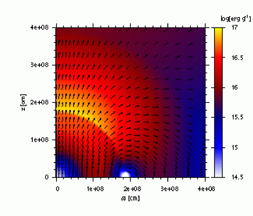
Figure 2.— Initial magnetic field configuration (vector) and distribution of specific magnetic energy in logarithmic scale for a representative model (Bs-$\Omega$-$\eta_{-\infty}$; see text). Note that all models share the same initial field configuration.

In each rotating model, an initial angular velocity is given by

$$\Omega(r)=\Omega_{0}\frac{r_{0}^{2}}{r_{0}^{2}+r^{2}}.$$ (86)

where $r_{0}=1000$ km and $\Omega_{0}=3.9$ rad s^-1.

Employing the above magnetic field and rotation, we study three different cases, namely, strong magnetic field and rapid rotation (model-series Bs-$\Omega$), moderate magnetic field and rapid rotation (model-series Bm-$\Omega$), and very strong magnetic field and no rotation (model-series Bss-$\mho$). Parameters for each model-series are given in Table 1.

Table 1Parameters and some results for the computed models.

Model name	$E_{\rm{m}}/W$ [%]	$T/W$ [%]	$j_{0}$ [cgs-Gauss]	$B_{0,\rm{i}}\tablenotemark{c}[G]$
Bs-Rot	0.5	0.5	$5.4\times 10^{14}$	$9.7\times 10^{12}$
Bm-Rot	0.05	0.5	$1.7\times 10^{14}$	$3.1\times 10^{12}$
Bss-Nonrot	5.0	0.0	$1.7\times 10^{15}$	$3.1\times 10^{13}$

In order to study effects of resistivity on the dynamics, both an ideal model and resistive models are run in each model-series. For the resistive models, we examine two different values of resistivity, say $\eta=10^{13}$ and $10^{14}$ cm² s^-1, reminding the discussion in § 1. Resistivity is uniform in space and time except that it is set zero inside the radius of 10 km to save the computational time. There a magnetic field and thus a resistivity are expected to be unimportant due to high density. For a descriptive convenience, we use abbreviations $\eta_{-\infty}$, $\eta_{13}$, and $\eta_{14}$, respectively, for models with $\eta=0$, $10^{13}$ and $10^{14}$ cm² s^-1, attaching after name of a model-series introduced above. For example, a model with strong magnetic field, rapid rotation, and $\eta=10^{14}$ cm² s^-1 is referred to as model Bs-$\Omega$-$\eta_{14}$.

Each computation is done in cylindrical coordinate. Assuming the axisymmetry and equatorial symmetry, we take the numerical domain as $(\varpi,z)\in[0~{}\textrm{km},4000~{}\textrm{km}]\times[0~{}\textrm{km},4000~{}\textrm{km}]$. Until the central density reaches $10^{12}$ g cm^-3, the number of numerical cells is $N_{\varpi}\times N_{z}=320\times 320$. After that the number of cells is changed to $N_{\varpi}\times N_{z}=720\times 720$. There, the spatial width of a cell increases outward in each direction with a constant ratio of 1.0051 and 1.0056, before and after the re-griding, respectively. Both the width $\Delta\varpi$ of the inner-most cells of $\varpi$-coordinate and the width $\Delta z$ of the inner-most cells of $z$-coordinate are 5 km and 400 m, before and after the re-griding, respectively. When the numerical cells are redistributed, physical variables are linearly interpolated from the coarse into the fine cells. In this procedure, the divergence-free constraint of magnetic field is usually violated, which stems from the poloidal components. To avoid this, we calculate $A_{\phi}$ from Eq. (85) using the distribution of $j_{\phi}$ right after the cell redistribution, and then obtain a divergence-free poloidal magnetic field.

Each simulation is run until the shock front reaches a radius of 2100, 3000, and 2300 km in model series Bs-$\Omega$, Bm-$\Omega$, Bss-$\mho$, respectively.

4. Results

In this section, we will present results of our computations for each model-series separately, seeing how a resistivity affect the dynamics of a magnetized supernova. Particular attentions are paid to the explosion energy, magnetic field amplification, and the aspect ratio of the ejecta.

Before proceeding to the main results, we here describe the dynamical evolution in the simulation without magnetic field and rotation. Soon after the start of computation, the core has a negative radial velocity everywhere, and collapses towards the center. A bounce occurs at $t=133$ ms due to nuclear force, and a shock wave is generated. The shock wave propagating outward first stalls around $r\sim 200$ km, but it starts gradual expansion around 165 ms. Afterward, the shock surface alternatly expands and shrinks. We followed the evolution until $t=350$ ms (217 ms after bounce) during which the maximum shock position is $\sim 800$ km. In this way, our model without magnetic field and rotation does not result in a stalled shock as seen recent core-collapse simulations (see e.g. Fig. 2 of Nordhaus et al. (2010)), which may be because we only consider a photo-dissociation of heavy nuclei but no neutrino cooling as cooling processes. Fig. 3 shows the evolutions of total, internal, gravitational, positive kinetic, and negative kinetic energies in the simulation without magnetic field. This indicates that a part of fluid has a positive radial velocity. Nontheless, we found that an estimated explosion energy is very small; less than $\sim 10^{48}$ erg and sometimes exactly zero. We assume that a fluid element is exploding if the total fluid energy plus the gravitational potential energy at its position, and the radial velocity are both positive, i.e. $e+\rho v^{2}/2+B^{2}/8\pi+\rho\Phi>0$ and $v_{r}>0$. Then the explosion energy is obtained by the sum of the total energy of fluid elements that fulfill the criterion plus the gravitational potential energy for the exploding fluid. We calculate the latter by $E_{\textrm{exp,grv}}=\int_{V_{\textrm{exp}}}[\rho\Phi_{\textrm{exp}}/2+\rho\tilde{\Phi}]dV$, where $\Phi_{\textrm{exp}}$ is the gravitational potential due to the exploding fluid and $\tilde{\Phi}$ is that due to the other fluid, and $\Phi=\Phi_{\textrm{exp}}+\tilde{\Phi}$. Gravitational potentials $\Phi_{\textrm{exp}}$ and $\tilde{\Phi}$ are obtained by solving a Poisson equation with only the mass of the exploding fluid and non-exploding fluid, respectively. The fact that the explosion enrgy is quite small as mentioned above implies that most or all fluid elements including those with a positive radial velocity do not fulfill the criterion. It seems reasonable to assume that the model without magnetic field and rotation does not explode.

The error in the total energy conservation of the system is 51 % at the end of the simulation. We found that the error in the total energy conservation is 24-33 % at the end of the all simulations involving magnetic field, except that it is 14 % in a different resolution run for model Bs-$\Omega$-$\eta_{14}$ described in § 4.1.5. In § 4.1.5, we will discuss whether these errors are problematic for results presented in this paper.

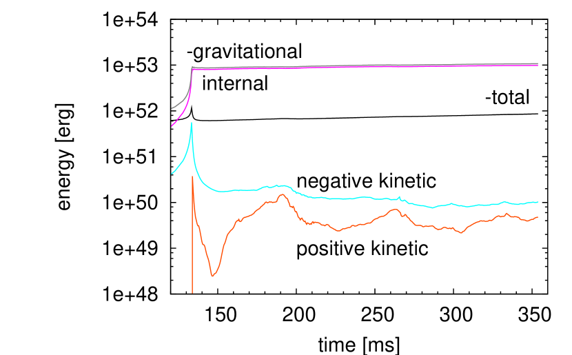
Figure 3.— Evolutions of the total (black line), internal (magenta), gravitational (gray), positive kinetic (orange), and negative kinetic (cyan) energy integrated over the whole numerical domain for the simulation without magnetic field and rotation. The total and gravitational energy are multiplied by $-1$.

4.1. Strong Magnetic Field and Rapid Rotation — Model Series Bs-$\Omega$

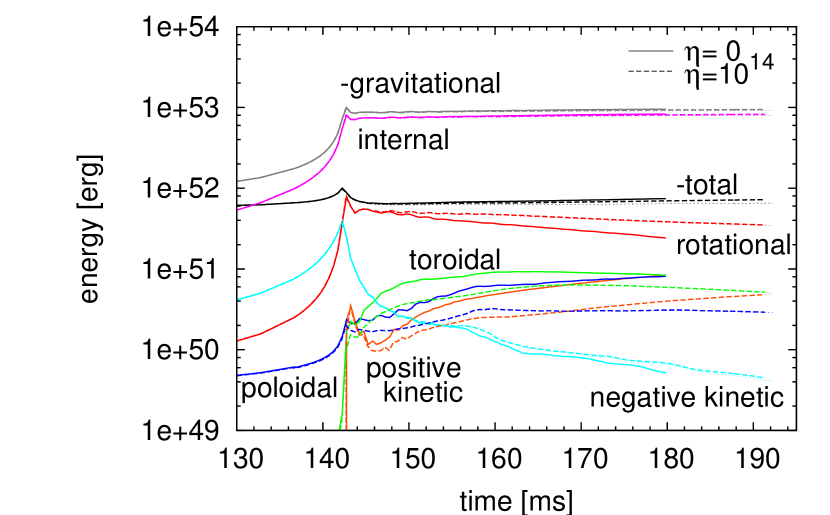
Figure 4.— Evolutions of the total (black lines), internal (magenta), gravitational (gray), rotational (red), positive kinetic (orange), negative kinetic (cyan), poloidal magnetic (blue), and toroidal magnetic (green) energy integrated over the whole numerical domain. The total and gravitational energy are multiplied by $-1$. The solid and dashed lines are drawn for model Bs-$\Omega$-$\eta_{-\infty}$ and Bs-$\Omega$-$\eta_{14}$, respectively. The dotted lines, which are almost identical with the dashed lines, are for a different resolution run for model Bs-$\Omega$-$\eta_{14}$ (see § 4.1.5)

We start from briefly describing the dynamical evolution in model Bs-$\Omega$-$\eta_{-\infty}$. In this model, a rotation hampers the collapse, and a bounce occurs at $t=143$ ms, 10 ms later than in the case without magnetic field and rotation. During the collapse, the core is largely spined up accompanied with an increase in the degree of differential rotation: Just after bounce, a rotational period reaches $\sim 1$ ms in a considerable part inside the radius of 50 km, while it is initially at least $\sim 1$ s. A magnetic field, which initially plays little role, is greatly amplified by compression during collapse. In addition, the differential rotation winds poloidal magnetic field-lines, and the toroidal component of magnetic field is largely generated around the time of bounce. An outward matter motion driven by bounce first decelerates, losing the energy due to a photo-dissociation of heavy nuclei, but accelerates again helped by a magnetic pressure of toroidal field and centrifugal force. As a result, a strong eruption of matter occurs preferentially along the pole. The above dynamical sequence can be followed in Fig. 4 in terms of energetics (see thick lines): i.e. a decrease of the gravitational energy results in an increase of the rotational and magnetic energy; the rotational energy is partially converted into the toroidal magnetic energy; then the toroidal magnetic energy is consumed to boost the positive kinetic energy. The top panels of Fig. 5 shows the distributions of velocity and magnetic field at 164 ms (21 ms after bounce) for model Bs-$\Omega$-$\eta_{-\infty}$. A fast mass eruption ($v_{r}\gtrsim 5\times 10^{9}$ cm s^-1) is seen notably around the pole, where the ratio of a magnetic pressure to matter pressure is large. This also implies that magnetic force plays an essential role for a fast mass eruption. Note that the dynamical features described here is quite similar to those found in previous works that employ similar strengths of magnetic field and rotation (see e.g. Yamada & Sawai (2004), Takiwaki et al. (2009)).

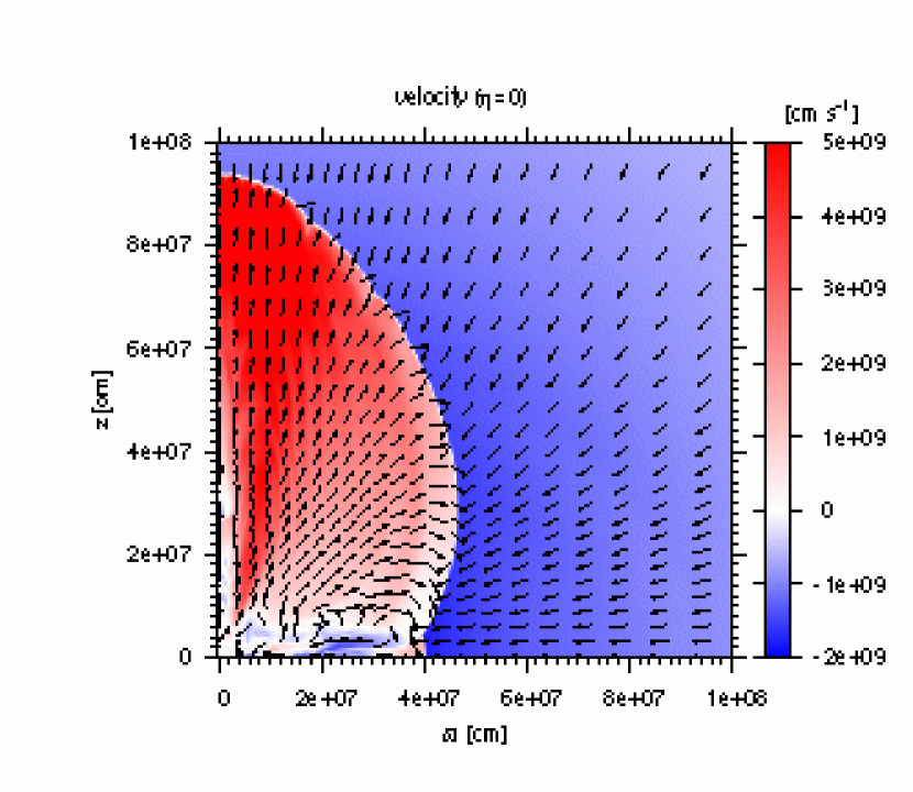
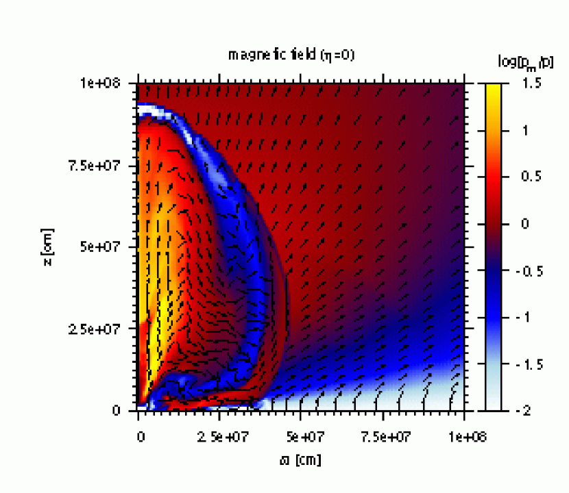
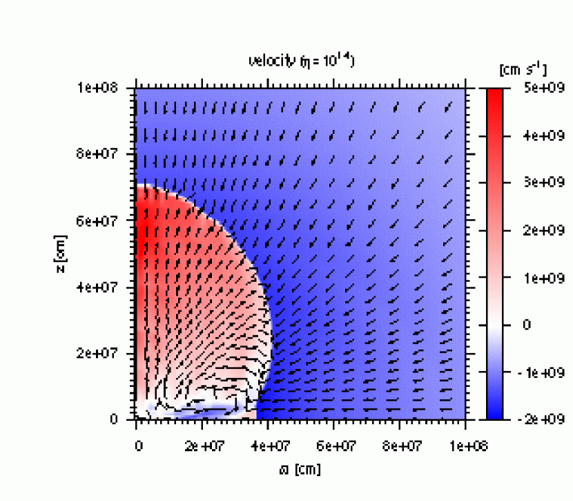
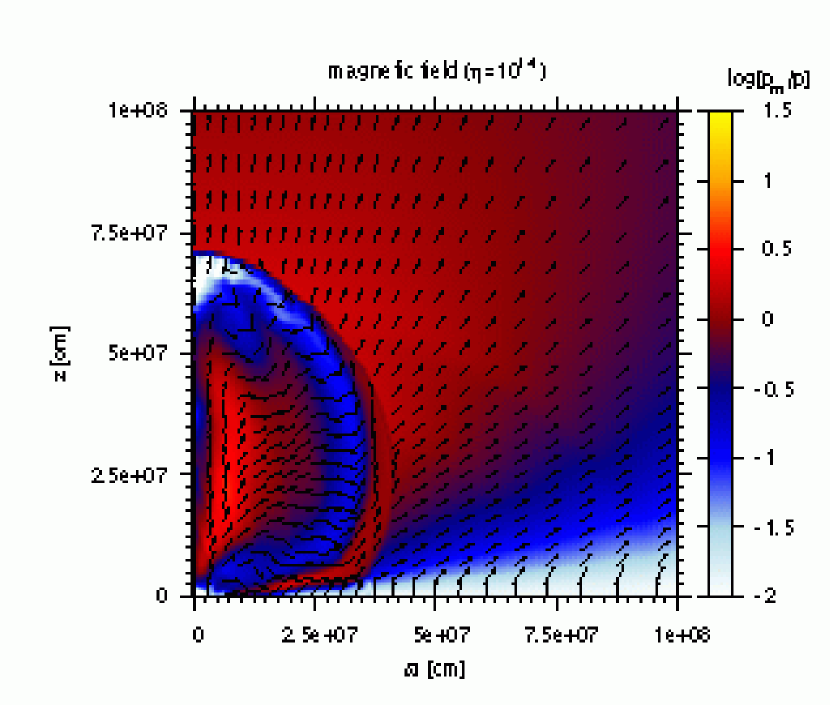
Figure 5.— Left panels: Distributions of radial velocity magnitude (color) and velocity direction (vectors). Right panels: Distributions of ratio of magnetic pressure to matter pressure, $p_{\textrm{m}}/p$, in logalithmic scale (color), and magnetic field direction (vectors). These figures are depicted at $t=164$ ms for model Bs-$\Omega$-$\eta_{-\infty}$ (upper panels) and Bs-$\Omega$-$\eta_{14}$ (lower panels).

In a resistive model Bs-$\Omega$-$\eta_{14}$, the evolution proceeds in qualitatively similar way to the ideal model Bs-$\Omega$-$\eta_{-\infty}$. However, outgoing velocities are relatively slow compared with the ideal model, which result in a smaller shock radius at a same physical time (compare the left panels of Fig. 5). The right panels of Fig. 5 implies that this is due to a less strong magnetic pressure in model $\eta_{14}$. As easily expected, a magnetic field amplification by differential rotation is ineffective under the presence of resistivity. This means that the rotational energy cannot be spent efficiently as an energy source for the explosion. Indeed, it is observed in Fig. 4 that the rotational energy in model $\eta_{14}$ decreases slowly compared with that of model $\eta_{-\infty}$ as well as both the positive kinetic and magnetic energy increase slowly.

4.1.1 Explosion Energy

Below, we will see the effect of resistivity on the explosion energy together with the detailed mechanism of the explosion. Fig. 6 shows the evolutions of the explosion energies, $E_{\textrm{exp}}$, in model-series Bs-$\Omega$. It is found that a larger resistivity results in a smaller explosion energy.

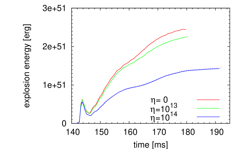
Figure 6.— Evolutions of the explosion energies in model-series Bs-$\Omega$. The red, green, and blue-solid lines are for model $\eta_{-\infty},\eta_{13},$ and $\eta_{14}$, respectively. The blue-dotted line is for a different resolution run for model Bs-$\Omega$-$\eta_{14}$ (see § 4.1.5). For the definition of an explosion energy, see text.

As a preparation for detailed analyses, we consider dividing the volume inside the shock surface into the two parts, say, the eruption-region and the infall-region. The definition of these parts are as follows. First, the volume inside the shock surface is equally cut up with respect to $\theta$ into 30 volume segments with $\Delta\theta=3^{\circ}$ opening angle. The eruption-region is defined by the sum of the segments whose integrated radial momentum is positive, whereas the infall-region is by the sum of those having the negative radial momentum. For example, in each left panel of Fig. 5, the infall-region appears in the vicinity of the equator ($\theta\gtrsim 70^{\circ}$) where a negative momentum dominates over a positive one, while the other part inside the shock surface corresponds to the eruption-region.

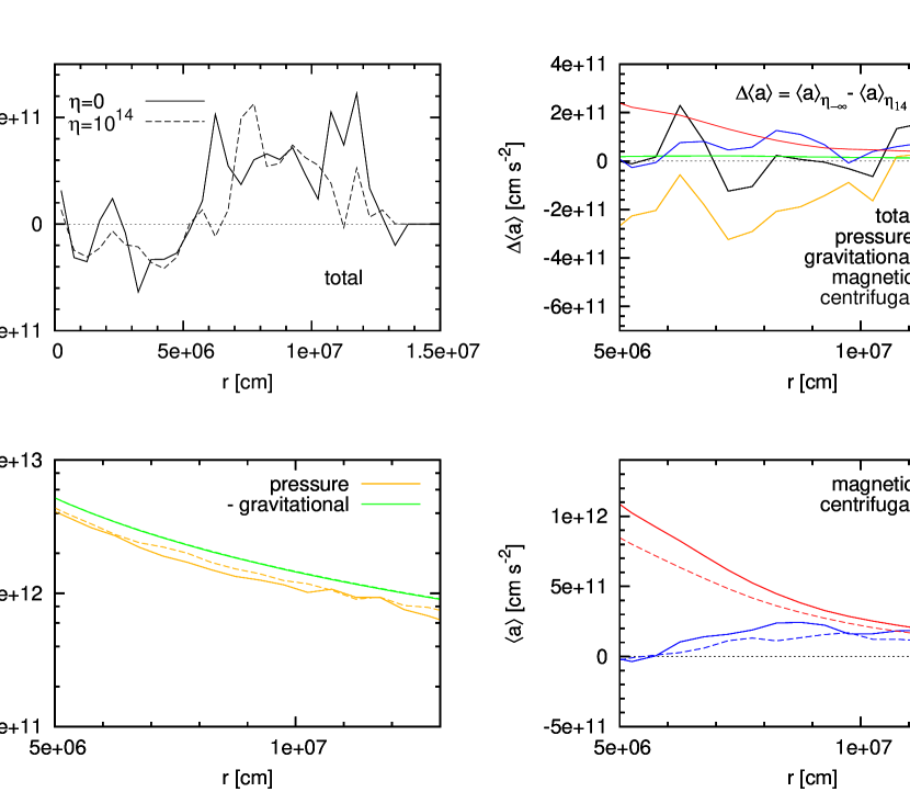
Figure 7.— Radial distributions of the radial accelerations, $\langle a\rangle$, angularly averaged in the eruption-region and time averaged during $t=147-155$ ms, in model Bs-$\Omega$-$\eta_{-\infty}$ and Bs-$\Omega$-$\eta_{14}$. In each panel, the black, red, blue, and magenta lines represent the total, pressure, gravitational, magnetic, and centrifugal accelerations, respectively. Except for the right-top panel, the solid lines are for model $\eta_{-\infty}$, while the dashed lines are for model $\eta_{14}$. The right-top panel shows the differences in the accelerations, $\Delta\langle a\rangle\equiv\langle a\rangle_{\eta_{-\infty}}-\langle a\rangle_{\eta_{14}}$, subtracting that of model $\eta_{14}$ from that of model $\eta_{-\infty}$.

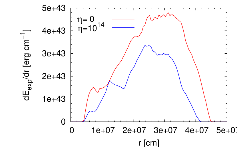
Figure 8.— Radial distributions of $dE_{\textrm{exp}}/dr$ at 155 ms in model Bs-$\Omega$-$\eta_{-\infty}$ and Bs-$\Omega$-$\eta_{14}$.

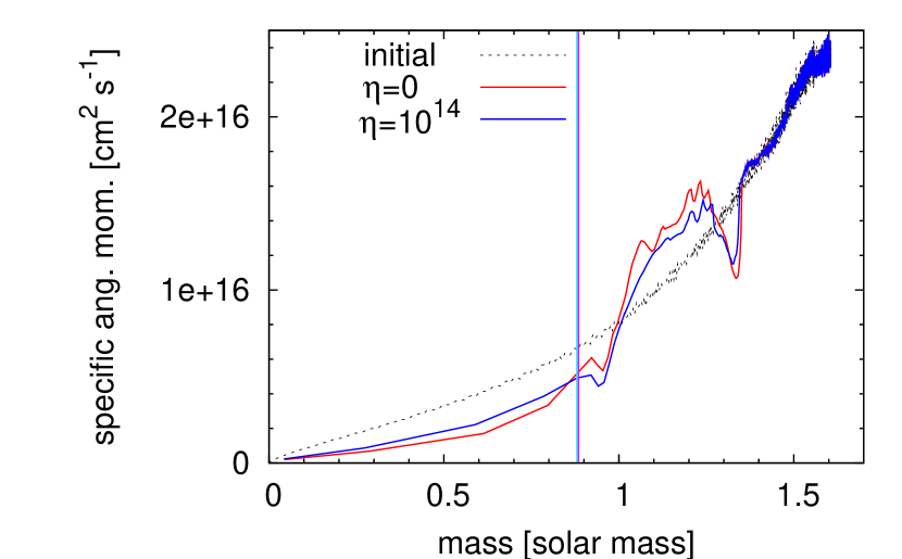
Figure 9.— Distributions of specific angular momentums in spherical mass coordinate at $t=155$ ms in model Bs-$\Omega$-$\eta_{-\infty}$ and Bs-$\Omega$-$\eta_{14}$. The Black-dashed line shows the initial distribution shared by the two models. The magenta and cyan vertical lines show the mass that corresponds to $r=25$ km, respectively, in model $\eta_{-\infty}$ and $\eta_{14}$.

To know what causes the differences in the explosion energy, it may be helpful to compare between model Bs-$\Omega$-$\eta_{-\infty}$ and Bs-$\Omega$-$\eta_{14}$ by the individual acceleration terms in the $r$-component of the equation of motion written on the frame rotating around the pole with the angular velocity $\Omega$;

$$\frac{D^{\prime}v_{r}}{Dt} = -\frac{1}{\rho}\frac{\partial p}{\partial r}-\frac{\partial\Phi}{\partial r}+\frac{1}{\rho c}\left(j_{\theta}B_{\phi}-j_{\phi}B_{\theta}\right)$$ (87)

$$+\Omega^{2}r\sin^{2}\theta,$$

where $D^{\prime}/Dt$ denotes the Lagrangian derivative on the rotating frame. In the r.h.s. of Eq. (87), each term represents, from left to right, the acceleration due to a pressure, gravity, magnetic field, and rotation. In comparing the accelerations, we take an angular average in the eruption-region and a time average during $t=t_{1}$ - $t_{2}$ ms, which are defined by

$$\langle a\rangle(r)=\int^{t_{2}}_{t_{1}}\left[\frac{\int_{\textrm{erup}}a\rho\sin\theta d\theta}{\int_{\textrm{erup}}\rho\sin\theta d\theta}\right]dt\bigg{/}\left[t_{2}-t_{1}\right],$$ (88)

where each term in the r.h.s. of Eq. (87) is to be assigned to $a$. Fig. 7 shows the radial distributions of accelerations, angularly averaged in the eruption-region and time averaged during $t=147$-$155$ ms, in model $\eta_{-\infty}$ and $\eta_{14}$. The averages are taken inside $\sim$140 km, the smallest shock radius at 147 ms in model $\eta_{-\infty}$ and $\eta_{14}$. It is found that, in the both models, an acceleration is almost everywhere positive for $r\gtrsim 50$ km (left-top panel). As shown in Fig. 8, a matter ejection also occurs roughly in this radial range, which implies that the amplitude of an acceleration is a good measure for the resulting magnitude of the explosion energy. There, a pressure acceleration alone is always smaller than a gravitational deceleration (left-bottom panel). The right-bottom panel shows that it is a magnetic and centrifugal acceleration that makes a matter ejection possible.

In the right-top panel of Fig. 7, the differences in accelerations between the two models are plotted, which shows that a total acceleration is averagely larger in model $\eta_{-\infty}$ for $r\gtrsim 50$ km. It is likely that this causes a larger $dE_{\textrm{exp}}/dr$ in model $\eta_{-\infty}$ as observed in Fig. 8. The right-top panel also indicates that a larger total acceleration in model model $\eta_{-\infty}$ is primary due to that in a magnetic and centrifugal acceleration. Although, a pressure acceleration is smaller in model model $\eta_{-\infty}$, this is more than compensated by them. Therefore, we conclude that a resistivity makes the explosion less energetic due to a small magnetic and centrifugal acceleration.

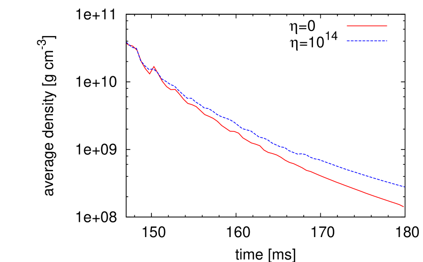
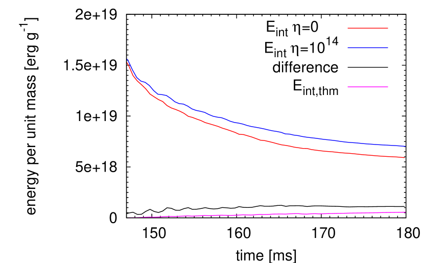
Figure 10.— Left: Evolution of the average density for $r>50$ km in the eruption-region in model Bs-$\Omega$-$\eta_{-\infty}$ and Bs-$\Omega$-$\eta_{14}$. Right: Evolution of the average specific internal energy for $r>50$ km in the eruption-region in model $\eta_{-\infty}$ (red line), model $\eta_{14}$ (blue), and the difference between them (black). The magenta line shows the time integrated Joule heating produced in the above region for model $\eta_{14}$.

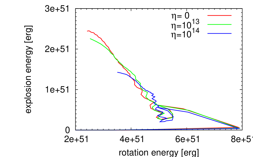
Figure 11.— Evolutions of the explosion energies in model-series Bs-$\Omega$ in terms of the remaining rotational energy. The evolution proceeds roughly in the counterclockwise direction.

While a smaller magnetic acceleration in model $\eta_{14}$ will be simply due to a weaker magnetic field as a result of a magnetic diffusion, that of centrifugal acceleration is related to a less efficient angular momentum transfer owing to a weaker magnetic stress. In Fig. 9, the distributions of specific angular momentums at 155 ms is plotted in mass coordinate. It is observed that a specific angular momentum in model $\eta_{14}$ is larger than that of model $\eta_{-\infty}$ inside the radius of $\sim 25$ km, whereas it is smaller outside there. This is the consequence of a less efficient outward angular momentum transfer in model $\eta_{14}$. Then, at a large radius, a centrifugal acceleration in model $\eta_{14}$ is smaller than that in model $\eta_{-\infty}$.

We also examined reasons for a larger pressure acceleration in model $\eta_{14}$ observed in the right-top panel of Fig. 7. In the present situation, a pressure is a increasing function of density and specific internal energy. Although a pressure also depends on electron fraction, this dependence is very weaker than that on the above two quantities. Hence, it is expected that the density or specific internal energy volume-averaged over the eruption-region are larger in model Ds-$\Omega$-$\eta_{14}$. By calculating these two average values, we found that both the average density and specific internal energy are larger for model $\eta_{14}$ (see Fig. 10). A higher density in model $\eta_{14}$ implies that the matter expansion rate is smaller, which is consistent with what is observed in the left panels of Fig. 5. A larger specific internal energy in model $\eta_{14}$ also may come from the smaller expansion rate, but may be caused by Joule heating too. To estimate an amount of thermal energy produced by Joule heating in model Ds-$\Omega$-$\eta_{14}$, the total heating rate of the eruption-region, $\int_{\textrm{erup}}4\pi\eta j^{2}/(\rho c^{2})dm$, is time-integrated from 147 ms when the infall-region begins to appear clearly. Then it is divided by a mass of the expulsion region at each instant of time, and compared with the difference in average specific internal energy between the two models. The result is shown in the right-panel of Fig. 10, which indicates that the contribution form the Joule heating to the difference in the specific internal energy is quite small around 150 ms. Thus, it is not likely that a larger pressure acceleration in model $\eta_{14}$ observed in the right-top panel of Fig. 7 is caused by Joule heating. A larger pressure acceleration seems to be just due to a smaller expansion rate in model $\eta_{14}$. The panel implies that only in a later phase, a larger specific internal energy in model $\eta_{14}$ may be somewhat contributed by the Joule heating. Note, however, that the thermal energy estimation made here may be crude, since a part of thermal energy produced in one region may migrate into another.

As we have seen, an inefficiency both in a magnetic field amplification and an angular momentum transfer leads to a weaker explosion in a resistive model. From the energetical point of view, this corresponds to an inefficiency in consuming the rotational energy as a fuel. Then one may think that the explosion energy of the ideal model and a resistive model would be similar compared in terms of the consumed rotational energy. If this is the case, the final explosion energy in the three models, after all the available rotational energy has been drained, would be comparable to each other. According to Fig. 11 this is not ture, however. In this figure the evolutions of the explosion energies in the three models are plotted against the remaining rotational energy. Since the maximum rotational energy, which is reached at the time of bounce, is almost same among the three models, $E_{\textrm{rot}}\approx 7.9\times 10^{51}$ erg, each model will consume roughly the same amount of rotational energy with a same position in the abscissa. It is found that the explosion energy in a resistive model is smaller than that of the ideal model, even though a same amount of rotational energy is expended. This implies that a part of the rotational energy is wasted in locations where the criterion for the explosion is not fulfilled.

4.1.2 Magnetic Field Amplification

In this section we analyze a magnetic field amplification. In Fig. 12, the angular distributions of the magnetic energies per unit mass, averaged over $50$ km$<r<0.9\times r_{\textrm{sh}}$ at $t=145$ ms (2 ms after bounce) and $t=160$ ms (17 ms after bounce), are shown for model Bs-$\Omega$-$\eta_{-\infty}$ and Bs-$\Omega$-$\eta_{14}$. The left panel indicates that the total magnetic energy is relatively stronger around the pole at 145 ms in each model, reflecting the initial magnetic field configuration (see Fig. 2). Turning to the right panel, it is found that, in each model, the contrast between the total magnetic energy around the pole and that around $\theta\sim 40^{\circ}$-$70^{\circ}$ becomes stronger at 160 ms than at 145 ms. In model $\eta_{14}$, the strong contrast in the total magnetic energy at 160 ms is mainly due to that in the toroidal magnetic energy, while in model $\eta_{-\infty}$, the contrast both in the toroidal and poloidal magnetic energies are responsible for that.

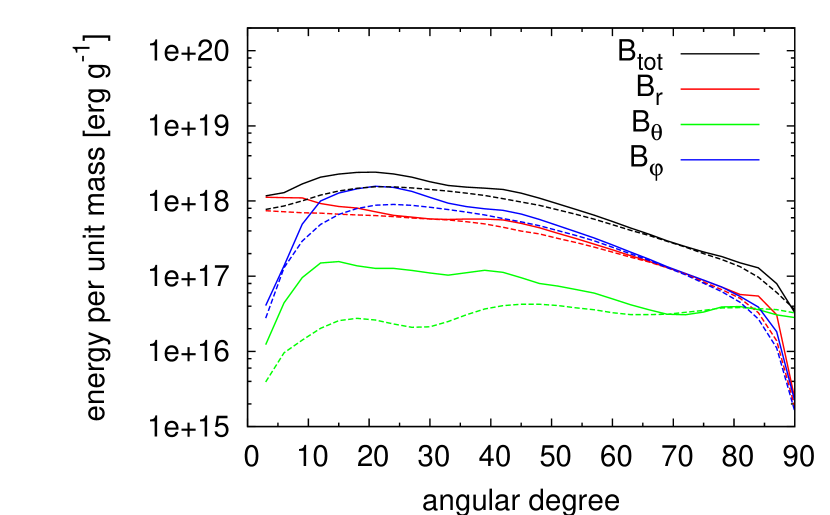
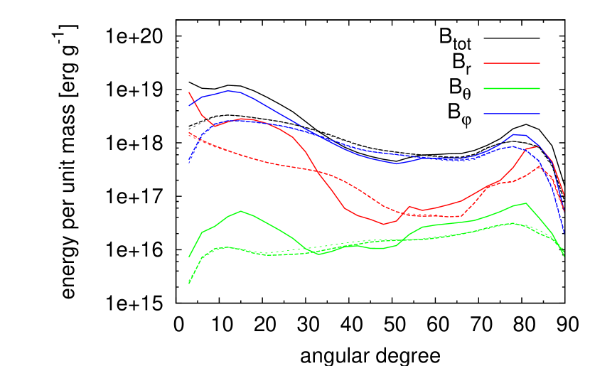
Figure 12.— Angular distributions of magnetic energies per unit mass averaged over $50$ km$<r<0.9\times r_{\textrm{sh}}$ at $t=145$ ms (2 ms after bounce; left) and $t=160$ ms (17 ms after bounce, right) in model Bs-$\Omega$-$\eta_{-\infty}$ (solid lines) and Bs-$\Omega$-$\eta_{14}$ (dashed lines). The dotted lines are for a different resolution run for model Bs-$\Omega$-$\eta_{14}$ (see § 4.1.5).

To understand how the contrast is strengthened, we follow the evolution of magnetic energy per unit mass in two representative volumes $V_{25.5}$ and $V_{58.5}$, where $V_{\theta_{\textrm{s}}}$ is defined by 50 km$\leq r\leq 0.9\times r_{\textrm{sh}}$ and $\theta_{\textrm{s}}-1^{\circ}.5\leq\theta\leq\theta_{s}+1^{\circ}.5$. Fig. 13 shows the evolution of the average magnetic energy per unit mass in the two volumes. It is observed both in model $\eta_{-\infty}$ and $\eta_{14}$, that the toroidal magnetic energy in the both volumes increases around 150 ms, and keeps an almost constant value afterward. The increase rate is higher in volume $V_{25.5}$. That is the contrast in the toroidal magnetic energy is strengthened around 150 ms, and is kept afterward. What is also found is that in model $\eta_{-\infty}$, the poloidal magnetic energy in volume $V_{25.5}$ increases during $t\sim 155$-$160$ ms, while that in volume $V_{58.5}$ does not vary very much. It seems that this makes the strong contrast in the poloidal magnetic energy in model $\eta_{-\infty}$ at 160 ms shown in the right panel of Fig. 12.

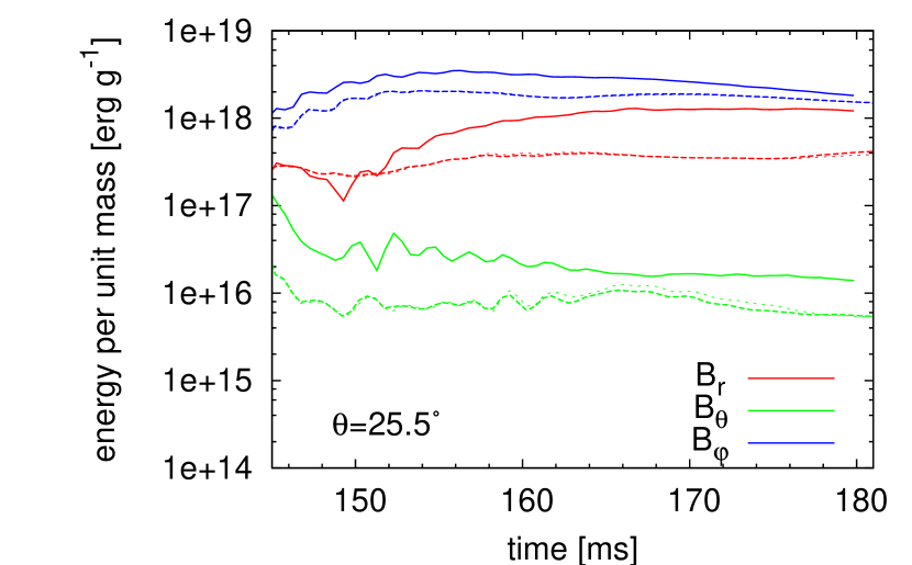
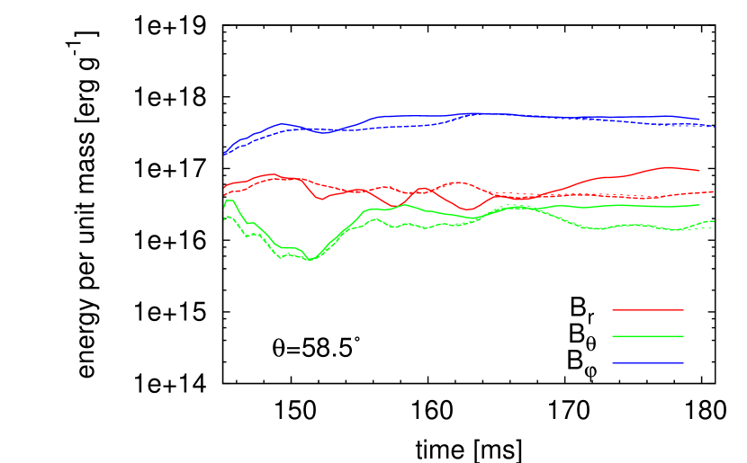
Figure 13.— Evolutions of average magnetic energies per unit mass of volume $V_{25.5}$ (left) and $V_{67.5}$ (right). The graphs are plotted from $t=145$ ms, 2 ms after bounce. The solid lines are for model Bs-$\Omega$-$\eta_{-\infty}$ while the dashed lines are for Bs-$\Omega$-$\eta_{14}$. The dotted lines are for a different resolution run for model Bs-$\Omega$-$\eta_{14}$ (see § 4.1.5).

In order to study the amplification mechanisms of magnetic field, we write down the evolution equations of the average magnetic energies per unit mass in volume $V_{\theta_{\textrm{s}}}$ with mass $M$, $\mathscr{E}_{\{r,\theta,\phi\}}=[\int(B_{\{r,\theta,\phi\}}^{2}/8\pi)dV]/M$:

$$\frac{d\mathscr{E}_{\{r,\theta,\phi\}}}{dt} = \phantom{+}\dot{\mathscr{E}}_{\{r,\theta,\phi\},\textrm{adv}}+\dot{\mathscr{E}}_{\{r,\theta,\phi\},\textrm{cmp}}+\dot{\mathscr{E}}_{\{r,\theta,\phi\},\textrm{shr}}$$ (89)

$$+\dot{\mathscr{E}}_{\{r,\theta,\phi\},\textrm{rst}}+\dot{\mathscr{E}}_{\{r,\theta,\phi\},\textrm{VM}},$$

where the terms in r.h.s. mean, from the left, the change of $\mathscr{E}_{\{r,\theta,\phi\}}$ due to an advection, compression, velocity shear along magnetic field lines, resistivity, and the variation in the volume and mass. They are defined by

$$\dot{\mathscr{E}}_{\{r,\theta,\phi\},\textrm{adv}} = -\frac{1}{M}\int\left[v_{r}\frac{\partial}{\partial r}+\frac{v_{\theta}}{r}\frac{\partial}{\partial\theta}\right]\frac{B_{\{r,\theta,\phi\}}^{2}}{8\pi}dV,$$

$$\dot{\mathscr{E}}_{r,\textrm{cmp}} = -\frac{1}{M}\int\left[\frac{2v_{r}}{r}+\frac{1}{r\sin\theta}\frac{\partial(\sin\theta v_{\theta})}{\partial\theta}\right]\frac{B_{r}^{2}}{4\pi}dV,$$

$$\dot{\mathscr{E}}_{\theta,\textrm{cmp}} = -\frac{1}{M}\int\left[\frac{1}{r}\frac{\partial(rv_{r})}{\partial r}+\frac{\cot\theta v_{\theta}}{r}\right]\frac{B_{\theta}^{2}}{4\pi}dV,$$

$$\dot{\mathscr{E}}_{\phi,\textrm{cmp}} = -\frac{1}{M}\int\left[\frac{1}{r}\frac{\partial(rv_{r})}{\partial r}+\frac{1}{r}\frac{\partial v_{\theta}}{\partial\theta}\right]\frac{B_{\phi}^{2}}{4\pi}dV,$$

$$\dot{\mathscr{E}}_{r,\textrm{shr}} = \hphantom{+[}\frac{1}{M}\int\frac{B_{r}B_{\theta}}{4\pi r}\frac{\partial v_{r}}{\partial\theta}dV,$$

$$\dot{\mathscr{E}}_{\theta,\textrm{shr}} = \hphantom{+[}\frac{1}{M}\int\frac{rB_{r}B_{\theta}}{4\pi}\frac{\partial(v_{\theta}/r)}{\partial r}dV,$$ (90)

$$\dot{\mathscr{E}}_{\phi,\textrm{shr}} = \hphantom{+[}\frac{1}{M}\int\left[B_{r}\frac{\partial(v_{\phi}/r\sin\theta)}{\partial r}+\frac{B_{\theta}}{r}\frac{\partial(v_{\phi}/r\sin\theta)}{\partial\theta}\right]$$

$$\hskip 12.0pt\times\frac{r\sin\theta B_{\phi}}{4\pi}dV,$$

$$\dot{\mathscr{E}}_{r,\textrm{rst}} = \hphantom{+[}\frac{\eta}{Mc}\int\frac{B_{r}}{r\sin\theta}\frac{\partial(\sin\theta j_{\phi})}{\partial\theta}dV,$$

$$\dot{\mathscr{E}}_{\theta,\textrm{rst}} = \hphantom{+[}\frac{\eta}{Mc}\int\frac{B_{\theta}}{r}\frac{\partial(rj_{\phi})}{\partial r}dV,$$

$$\dot{\mathscr{E}}_{\phi,\textrm{rst}} = -\frac{\eta}{M}\int\left[\frac{\partial(rj_{\theta})}{\partial r}-\frac{\partial j_{r}}{\partial\theta}\right]\frac{4\pi}{c}\frac{B_{\phi}}{r}dV,$$

$$\dot{\mathscr{E}}_{\{r,\theta,\phi\},\textrm{VM}} = \hphantom{+[}\frac{\ointop\left(B_{\{r,\theta,\phi\}}^{2}/8\pi\right)\mbox{\boldmath$v$}_{\textrm{srf}}\cdot d\mbox{\boldmath$S$}}{M}$$

$$-\frac{\int\left(B_{\{r,\theta,\phi\}}^{2}/8\pi\right)dV}{M^{2}}\frac{dM}{dt},$$

where $\mbox{\boldmath$v$}_{\textrm{srf}}$ is a surface velocity of volume $V_{\theta_{\textrm{s}}}$. Note that the resistive terms are written for a constant resistivity. By evaluating these terms we can see which factors are essential for the magnetic field amplification in a given volume. The results are shown in Fig. 14 and 15.

We first focus on the amplifications of the toroidal magnetic energies in model $\eta_{-\infty}$. In volume $V_{25.5}$, the toroidal magnetic energy is primarily amplified by an advection (right-top panel of Fig. 14). We found that an radial advection dominates over an angular advection, i.e. the amplification is due to an outward advection of a large toroidal energy at small radii. As expected, a velocity shear along poloidal magnetic field-lines, viz. a winding due to a differential rotation, also substantially contributes to the amplification. In volume $V_{58.5}$, the toroidal magnetic energy is also amplified due to an advection and shear (see the right-bottom panel of Fig. 14), but the amplitude of each term is much smaller than in volume $V_{25.5}$, which seems due to a priori weaker magnetic field.

The amplification of the radial magnetic energy in volume $V_{25.5}$ is also dominated by a radial advection. The shear term, which is far smaller than that of the advection term, seems to also play an important role after $\sim 160$ ms, since it is comparable to a total $\dot{\mathscr{E}}$ (see the left-top panel of Fig. 14). As seen in the left-bottom panel of Fig. 14, the amplification mechanism of radial magnetic energy in the volume $V_{58.5}$ is rather complex, contributed by several terms. As in the case of a toroidal magnetic energy, an amplification of a radial magnetic energy is also weaker in volume $V_{58.5}$ than in volume $V_{25.5}$.

Since the present model-series involves a rotation, the magnetorotational instability (MRI) may occur and may play an important role in a magnetic field amplification (Balbus & Hawley, 1991; Akiyama et al., 2003; Masada et al., 2006). Signs for MRI growth is found in some of past MHD core-collapse simulations initially assuming a magnetar-class magnetic field (Yamada & Sawai, 2004; Takiwaki et al., 2004; Obergaulinger et al., 2006; Shibata et al., 2006). Also, Obergaulinger et al. (2009) carried out simulations of MRI with a rather weak initial magnetic field, which is still stronger than that of ordinary pulsars by an order of magnitude, using a local simulation box, and found that the MRI exponentially amplifies the seed magnetic field. Note however that the effect of accretion is not considered in their local box simulations. According to Foglizzo et al. (2006), the neutrino-driven convection in the gain region can be stabilized or slowed down by accretion. This may also hold for the MRI in the post-shock region.

We investigated whether, in model $\eta_{-\infty}$ and $\eta_{14}$, there emerges a region where the criterion for the MRI (Balbus, 1995) is satisfied and the growth timescale is short enough. In the left-top panel of Fig. 16, we plot the distribution of a MRI linear growth timescale, roughly estimated by $4\pi/|\varpi d\Omega/d\varpi|$, in $\theta$-$r$ plane at $160$ ms (17 ms after bounce) for model $\eta_{-\infty}$. It is shown that in a considerable part for $\theta\lesssim 40^{\circ}$, the growth timescale of MRI is a few ms to 10 ms, while in a larger $\theta$ the growth timescale is averagely longer. We found that, in the above part, the growth timescale of $\sim$10 ms is kept after bounce ($t=143$ ms) until the end of the simulation. However, the right-top panel of Fig. 16 does not shows MRI-like field-line bending as observed in some models in Yamada & Sawai (2004) (model MF3 and MF8). This may be because the present model leads to a stronger matter eruption in the radial direction than those models of Yamada & Sawai (2004) because of a rather mild initial rotation speed. In the present model, field-line bending produced by the MRI may become invisible due to a dominant radial flow, and the absence of that will not necessarily mean the non-operation of the MRI. Note that the absence of field-line bending seems not due to a poor spacial resolution: A field-line bending is observed even in the computations of model-series Bm-$\Omega$, in which a magnetic field is averagely weaker than in the present case and thus the resolution for capturing MRI is poorer. In the present case, the fastest growing wave length is resolved everywhere with several 10 numerical cells (see the bottom panels of Fig. 16). Although the required number of numerical cells to capture one wave length depends on numerical scheme, several 10 cells will be sufficient.

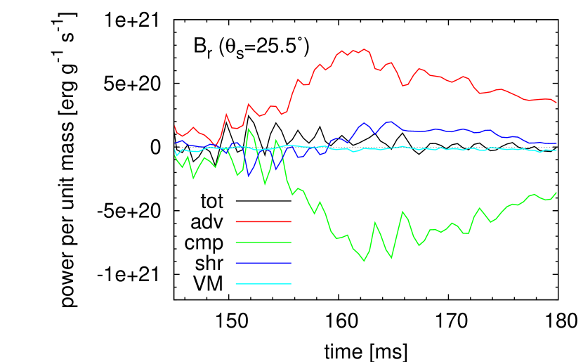
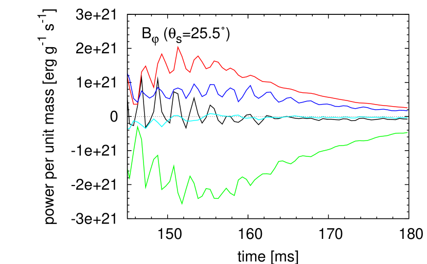
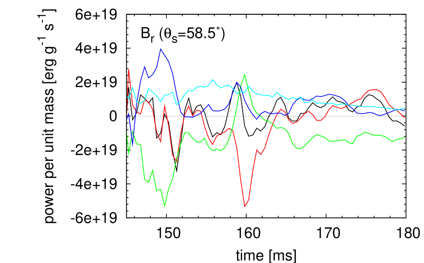
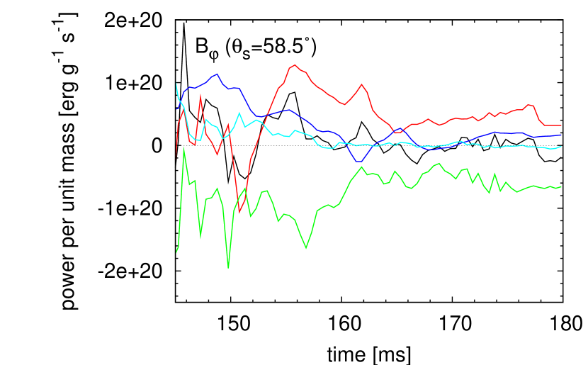
Figure 14.— Evolution of each $\dot{\mathscr{E}_{r}}$ and $\dot{\mathscr{E}_{\phi}}$ (see Eq. (4.1.2)) in volume $V_{25.5}$ and $V_{58.5}$ in model Bs-$\Omega$-$\eta_{-\infty}$.

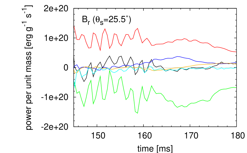
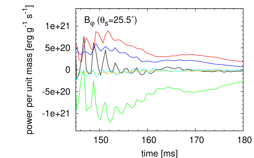
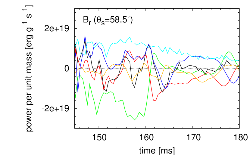
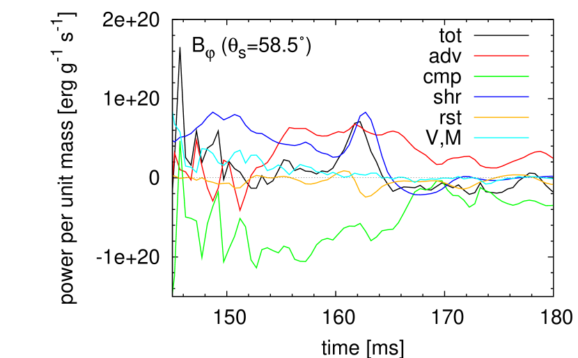
Figure 15.— Same as Fig. 14 but for Bs-$\Omega$-$\eta_{14}$. Note that the vertical scale of each panel in Fig. 14 and 15 are different except for the right-bottom panel.

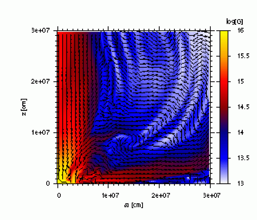
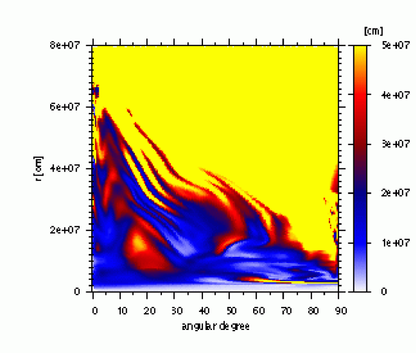
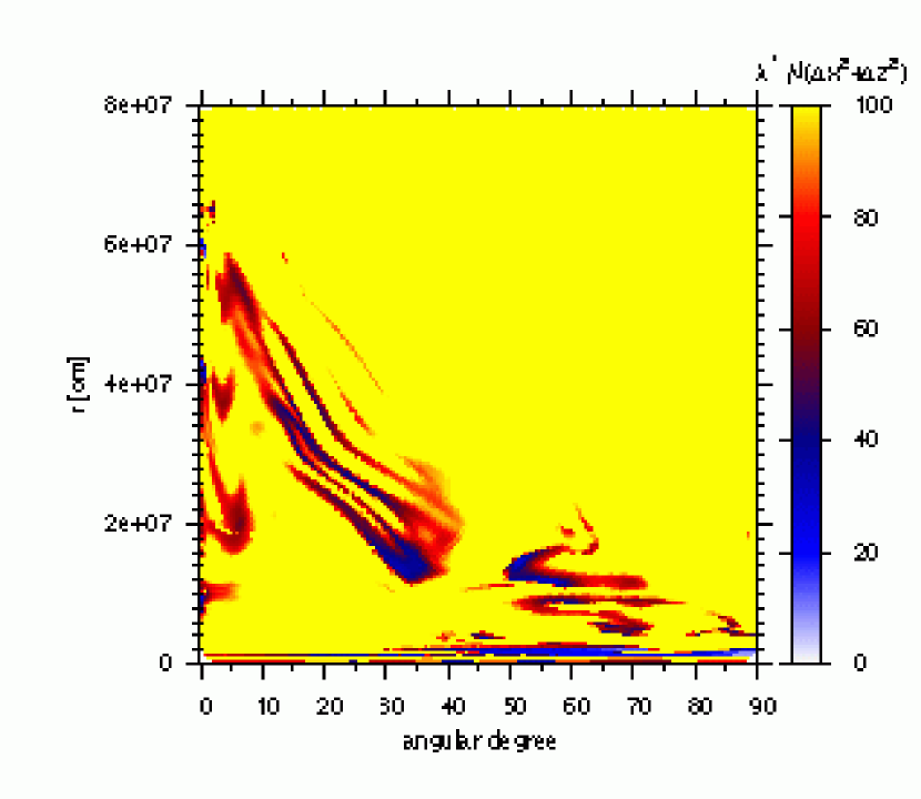
Figure 16.— Left-top panel: Distribution of MRI growth timescale in logarithmic scale in $\theta$-$r$ plane. White-colored regions include a location that is stable against the MRI. Right-top panel: Poloidal magnetic field vectors on top of a color map of poloidal magnetic field strength. Left-bottom panel: Distribution of fastest growing wave length, $\lambda^{*}\sim 2\pi c_{\textrm{A}}/\Omega$, where $c_{\textrm{A}}$ is the Alfvén velocity of a poloidal magnetic field. Right-bottom panel: Distribution of fastest growing wave length divided by numerical cell size, $\lambda^{*}/\sqrt{(\Delta x)^{2}+(\Delta z)^{2}}$. Yellow-colored region includes MRI-stable locations. These figures are depicted for model Bs-$\Omega$-$\eta_{-\infty}$ at $t=160$ ms.

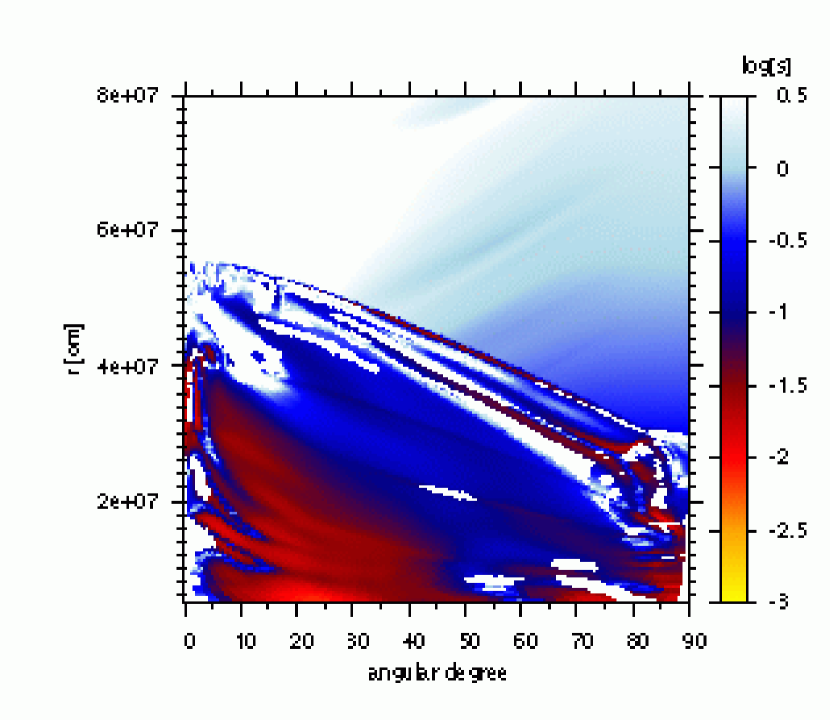
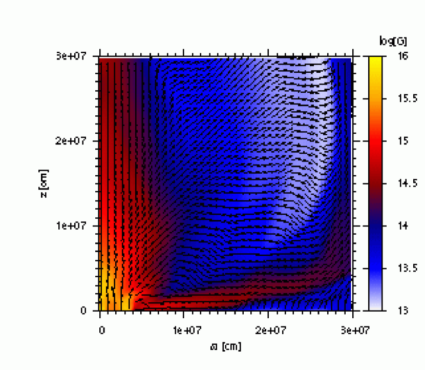
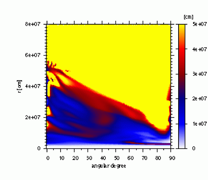
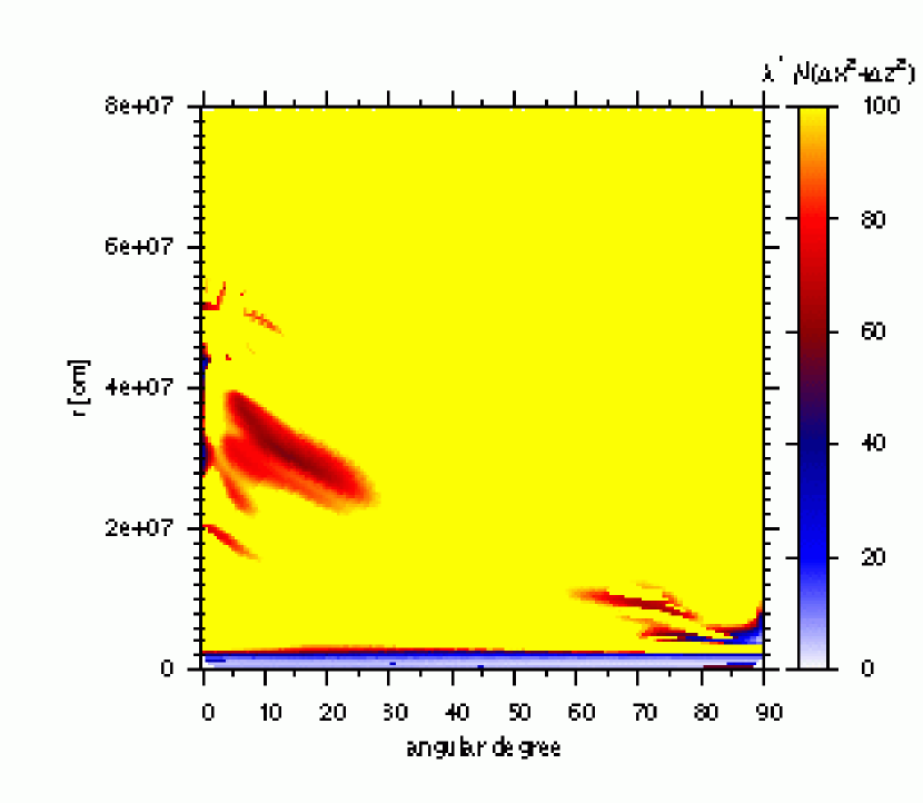
Figure 17.— Same as Fig. 16 but for model Bs-$\Omega$-$\eta_{14}$ at $t=160$ ms.

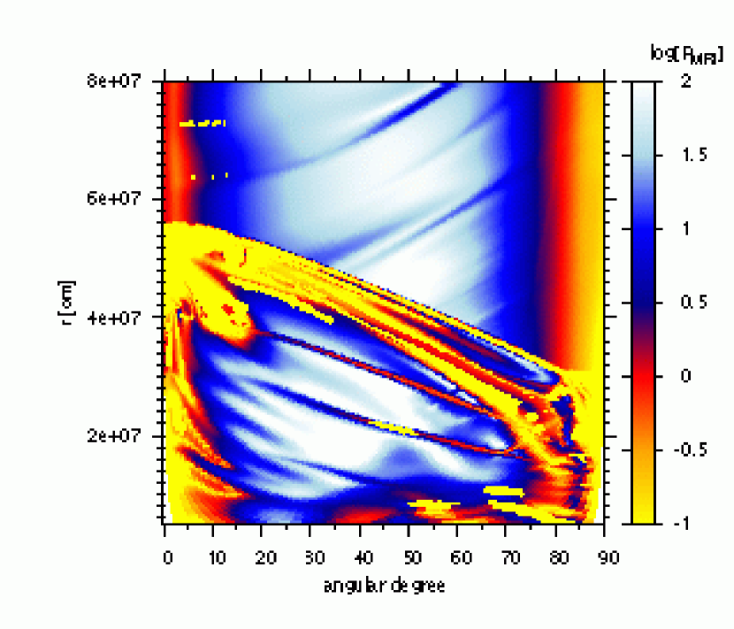
Figure 18.— Distribution of $R_{\textit{MRI}}\equiv\tau_{\textrm{res}}/\tau_{\textrm{MRI}}$, in logarithmic scale in $\theta$-$r$ plane in model Bs-$\Omega$-$\eta_{14}$ at $t=160$ ms.

The growth of the MRI will lead to an increase of the shear term in Eq. (89), since the MRI produce a shear of velocity along a magnetic field-line. The left panel of Fig. 14 shows that the shear term in volume $V_{25.5}$ becomes relatively large after $\sim 160$ ms ($\sim 20$ ms after bounce). Given that the MRI growth timescale there is $\sim 10$ ms, it may be reasonable to consider that the increase of the shear term is due to the operation of MRI. Even if this is the case, however, it is unlikely that the MRI greatly amplifies a magnetic field, since the radial magnetic energy is nearly constant after $\sim 160$ ms (see left panel of Fig. 13). The MRI seems at best to keep the strength of magnetic field in volume $V_{25.5}$. Since the fastest MRI growth timescale is comparable at each $\theta$ for $\theta\lesssim 40^{\circ}$, the situation will be more or less similar in this angular range.

Meanwhile, in the angular range of $\theta\gtrsim 40^{\circ}$, even the retention of magnetic field strength by the MRI will be modest, because a growth timescale reaches $\sim 10$ ms only in some limited locations (see the left-top panel of Fig. 16). Although, in volume $V_{58.5}$, the shear term helps to increase or keep the radial magnetic energy (the left-bottom panel of Fig. 14), this begins long before the MRI is expected to grow. Only in later time (e.g. after $\sim 160$ ms), the shear term might contain some modest contribution from the MRI.

The amplification mechanism in model $\eta_{14}$ is qualitatively similar to that in model $\eta_{-\infty}$, although the amplitude of each $\dot{\mathscr{E}}$ is usually smaller due to resistivity (see Fig. 15). The left-top panel of Fig. 17 plotted for $t=160$ ms shows that in a considerable part for $\theta\lesssim 45^{\circ}$, the MRI growth timescale is 10 ms to a few 10 ms, which is kept from the time of bounce (143 ms) until the end of the simulation. Fig. 18 displays the distribution of resistive timescale divided by MRI growth timescale, $R_{\textit{MRI}}\equiv\tau_{\textrm{res}}/\tau_{\textrm{MRI}}$, at 160 ms. This indicates that the growth of the MRI is more or less hampered by a resistivity. Especially, in the vicinity of the pole, there is almost no chance for the MRI growth. We found that, the growth of MRI is possible through the simulation in the angular range of $20^{\circ}\lesssim\theta\lesssim 30^{\circ}$, although a growth rate will be somewhat decreased by a resistivity in some locations (blue-colored regions for $20^{\circ}\lesssim\theta\lesssim 30^{\circ}$ in Fig. 18). In this model, the fastest growing wave length is resolved with several 10 numerical cells everywhere except for $r<20$ km (see bottom panels of Fig 17).

The left-top panel of Fig. 15 also shows that the shear term in volume $V_{25.5}$ becomes large after $\sim 160$ ms. By the same discussion done in the above, this is possibly due to the MRI, but not important for a magnetic field amplification. Again, the MRI at best may contribute to keep the radial magnetic energy in model $\eta_{14}$.

In light of the above discussion, it can be said that the contrast in magnetic energy per unit mass over $\theta$ observed both in model $\eta_{-\infty}$ and $\eta_{14}$ is strengthened or kept by an outward advection of magnetic energy, winding of poloidal magnetic field-lines, and possibly by the MRI, all of which efficiently occur in a small-$\theta$ region.

4.1.3 Aspect Ratio

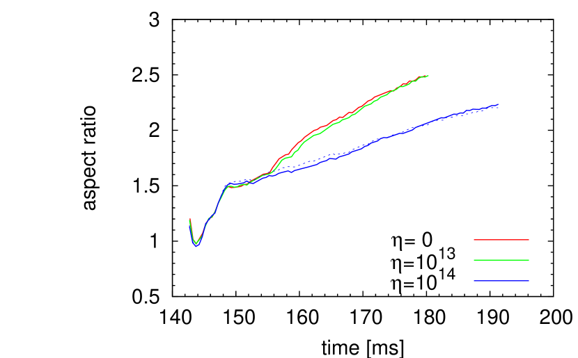
Figure 19.— Evolutions of aspect ratios (left panel) and the maximum ejecta positions in $z$ and $\varpi$ (right panel) in model-series Bs-$\Omega$. The dotted line in the left panel is for a different resolution run for model Bs-$\Omega$-$\eta_{14}$ (see § 4.1.5).

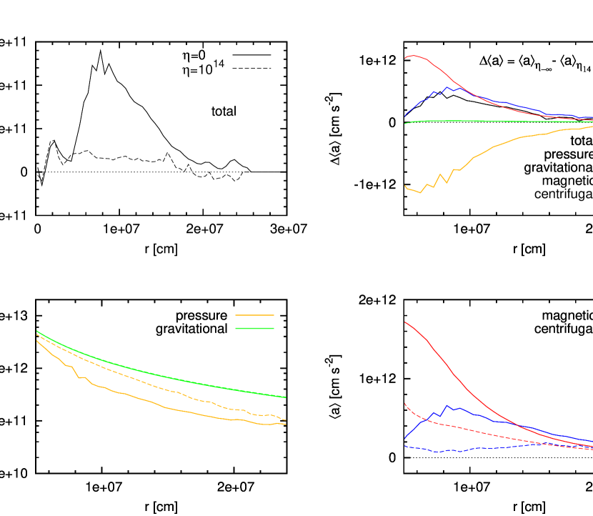
Figure 20.— Radial distributions of the accelerations in volume $V_{25.5}$, $\langle a\rangle$, time averaged during $t=155-165$ ms, in models Bs-$\Omega$-$\eta_{-\infty}$ and Bs-$\Omega$-$\eta_{14}$. The right-top panel shows the differences in the accelerations, $\Delta\langle a\rangle\equiv\langle a\rangle_{\eta_{-\infty}}-\langle a\rangle_{\eta_{14}}$, subtracting that of model $\eta_{14}$ from that of model $\eta_{-\infty}$. Colors and styles of lines are same as in Fig. 7

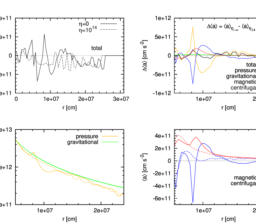
Figure 21.— Same as Fig. 20, but for volume $V_{58.5}$

From Fig. 5 it is found that the shape of the shock surface is prolate both in model Bs-$\Omega$-$\eta_{-\infty}$ and model Bs-$\Omega$-$\eta_{14}$, in which the latter shows a less prolate feature than the former. Defining the aspect ratio by the maximum-$z$ position of ejected matters, $z_{\textrm{ej,max}}$, divided by the maximum-$\varpi$ position, $\varpi_{\textrm{ej,max}}$, we found that it exceeds two at the end of each simulation (see Fig. 19).

We first focus on the aspect ratio in model $\eta_{-\infty}$. Fig. 19 indicates that the aspect ratio becomes larger than unity soon after bounce ($t=143$ ms). Since a centrifugal force is relatively stronger around the equator, it hampers the collapse and weakens the bounce there. This is one reason for the prolate matter ejection. Figs. 20 and 21 shows the radial distributions of the accelerations, time averaged during $t=155$-$165$ ms, in volume $V_{25.5}$ and $V_{58.5}$, respectively. It is found that in volume $V_{25.5}$, a matter is greatly accelerated in the radial range of 50 km$\lesssim r\lesssim$160 km (see solid line in the left-top panel of Fig. 20). Meanwhile, in volume $V_{58.5}$, an acceleration of matter is averagely smaller (see solid line in the left-top panel of Fig. 21). This implies that an acceleration of matter is larger for a smaller $\theta$, which causes a further increase of the aspect ratio. Comparing the bottom panels of the two figures, a larger magnetic and centrifugal acceleration in volume $V_{25.5}$ seems responsible for the larger acceleration. Reminding that a stronger magnetic field leads to a larger amplitudes of these two accelerations (see § 4.1.1), it is likely that a polarly concentrated distribution of magnetic energy per unit mass (§ 4.1.2) is essential to generate a large aspect ratio.

Comparing the aspect ratio among the three models in the left panel of Fig. 19, it is the smallest in model $\eta_{14}$, while that in models $\eta_{-\infty}$ and $\eta_{13}$ takes similar value. The right panel of Fig. 19 shows that the difference comes from the fact that $z_{\textrm{ej,max}}$ is largely affected by resistivity, while $\varpi_{\textrm{ej,max}}$ does not change so much. With this and the above speculation that a prolate matter ejection is caused by a polarly concentrated magnetic energy distribution, the smaller aspect ratio in model $\eta_{14}$ is readily understood. In Fig. 20, it is shown that a total acceleration in volume $V_{25.5}$ is smaller in model $\eta_{14}$ due to smaller contribution from a magnetic and centrifugal acceleration. Meanwhile, a total acceleration in volume $V_{58.5}$ is not very different between the two models (see Fig. 21), because a magnetic and centrifugal acceleration are not as important as in volume $V_{25.5}$ due to a small magnetic energy per unit mass. This leads to a large difference only in $z_{\textrm{ej,max}}$, and thus in the aspect ratio.

4.1.4 Diffusion and Dissipation Sites

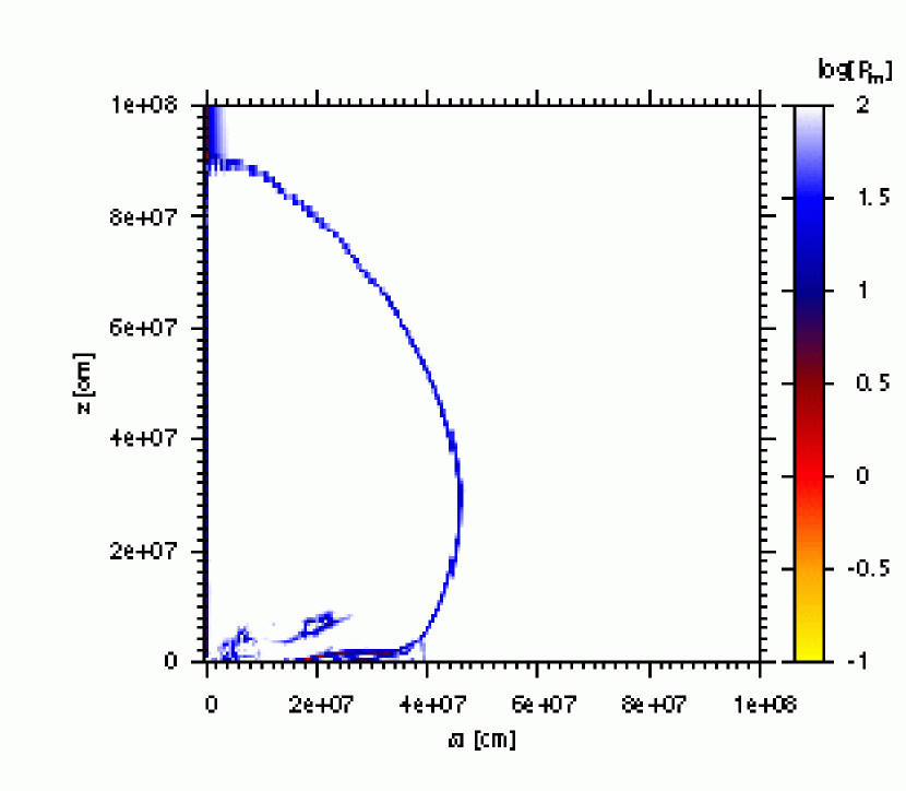
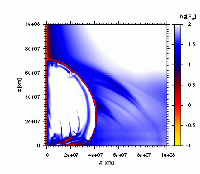
Figure 22.— Distributions of magnetic Reynolds number $R_{\textrm{m}}$ in logarithmic scale at $t=164$ ms in model Bs-$\Omega$-$\eta_{13}$ (left) and Bs-$\Omega$-$\eta_{14}$ (right).

In this section, we will see in which sites a resistivity works efficiently. In Fig. 22, the distribution of magnetic Reynolds number $R_{\textrm{m}}$, the ratio of the resistive timescale to dynamical timescale, in model Bs-$\Omega$-$\eta_{13}$ and Bs-$\Omega$-$\eta_{14}$ are displayed for $t=164$ ms. We define the resistive and dynamical timescales, respectively, by $L^{2}/\eta$ and $|L\mbox{\boldmath$B$}|/|\mbox{\boldmath$v$}\times\mbox{\boldmath$B$}|$, where the scale length of magnetic field is defined by $L\equiv|c\mbox{\boldmath$B$}|/|4\pi\mbox{\boldmath$j$}|$. With these definitions, the magnetic Reynolds number is also the ratio of the size of the first term to second term in r.h.s. of Eq. (5). If we define a diffusion-dissipation site by the location where the magnetic Reynolds number is $\lesssim$100, the right panel of Fig. 22 shows that the diffusion-dissipation sites in model $\eta_{14}$ are, around the pole, equator, the shock surface and in the blue filaments inside the shock surface. In these sites, a magnetic Reynolds number is small since the scale length of magnetic field is short: that of toroidal field is short around the pole, while that of poloidal field is short in the other sites. Comparing the right panels of Fig. 5, an intense magnetic pressure dominance seen around the pole in model $\eta_{-\infty}$ are not found in model $\eta_{14}$. This implies that a diffusion and dissipation around the pole are essential for producing the dynamical differences between model $\eta_{-\infty}$ and $\eta_{14}$.

In the case of model $\eta_{13}$, a resistivity works efficiently also around the pole, equator, and the shock surface, but the volumes of these sites are much smaller than those in the former case due to a lower resistivity. Besides, a magnetic Reynolds number there is generally at least $\sim 30$, although in some very limited regions it reaches an order of unity. Hence, model $\eta_{13}$ is rather close to the ideal model. With this the explosion energy and aspect ratio in model $\eta_{13}$ are not much different from those in model $\eta_{-\infty}$.

4.1.5 Convergences of Results

As a final remark for models-series Bs-$\Omega$, we mention the convergences of results with respect to the size of the numerical cells. As a representative model, we carry out another run for model Bs-$\Omega$-$\eta_{14}$ with a different spatial resolution. Keeping the total number of cells, the size of the inner-most cells is changed from $400$ m to $200$ m, where a cell size increases outwards both in $\varpi$ and $z$-direction with the constant ratio of 1.0069. With this distribution a resolution is higher than the original one for $z,\varpi<200$ km, and lower otherwise. In Figs. 4, 6, 12, 13, and 19, the results obtained with this different resolution are shown for model Bs-$\Omega$-$\eta_{14}$ by dotted lines. Although a little deviations from the original results are observed in some figures, they seem not to qualitatively and even quantitatively affect the discussions given above.

The error in the total energy conservation in the different resolution run is 14 % as mentioned at the beginning of § 4. That in the normal resolution run of model Bs-$\Omega$-$\eta_{14}$, 26 %, is roughly twice as large as the different resolution one. Nonetheless, as we have seen, only slight deviations are found between results of the two resolution run. Hence, although the total energy error of 26 % may be a little too large, this will not spoil the results of the simulation. We expect that this is also the case for the other models.

4.2. Moderate Magnetic Field and Rapid Rotation — Model Series Bm-$\Omega$

The dynamical evolutions in model-series Bm-$\Omega$ is qualitatively similar to those found in model-series Bs-$\Omega$, i.e. a winding of magnetic field-lines by a differential rotation increases a magnetic and centrifugal acceleration, which play a key role in a matter ejection. Owing to a weaker initial magnetic field, the explosion occurs less energetically than in the former model-series. The distributions of velocity and magnetic field at $t=181$ ms in model Bm-$\Omega$-$\eta_{-\infty}$ and Bm-$\Omega$-$\eta_{14}$ are depicted in Fig. 23. Compared to model-series Bs-$\Omega$ with a same resistivity (see Fig. 5), the present model-series shows a slower outward velocity and an averagely weaker magnetic pressure. As in the former model-series, a comparison between the upper and lower panels of Fig. 23 also indicates that an matter eruption becomes weaker with the presence of resistivity, with which we expect a lower explosion energy for a resistive model.

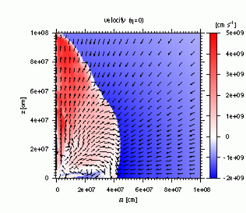
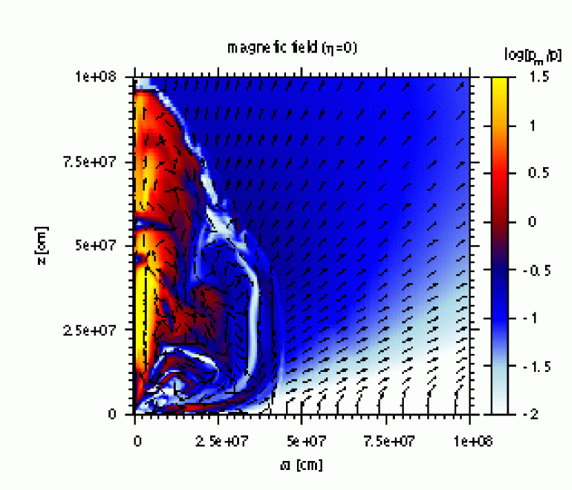
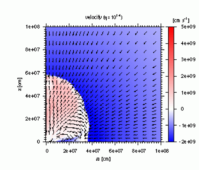
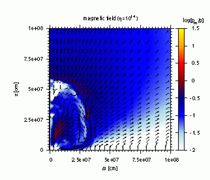
Figure 23.— Same as Fig. 5 but for model Bm-$\Omega$-$\eta_{-\infty}$ (upper panels) and Bm-$\Omega$-$\eta_{14}$ (lower panels) depicted at $t=181$ ms.

4.2.1 Explosion Energy

Fig. 24 plots the evolutions of the explosion energies in the present model-series. The resulting explosion energy in each model appears to be about factor three smaller than the corresponding model in model-series Bs-$\Omega$. It is shown that a resistivity also decreases the explosion energy as in the former case. This can be understood same way as we have seen in § 4.1.1 for model-series Bs-$\Omega$.

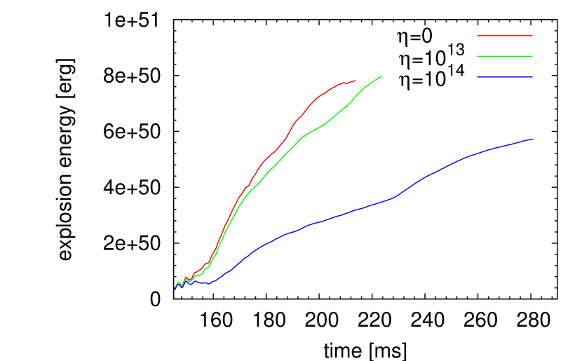
Figure 24.— Evolutions of explosion energies in model-series Bm-$\Omega$.

Fig. 25 shows the radial distribution of accelerations, angularly averaged in the eruption-region and time averaged during 160-170 ms, according to Eq. (88). The left-top panel shows that an acceleration of matter mainly takes place around $r\sim 100$ km. There, although a pressure acceleration alone does not overcome an inward gravitational acceleration (see the left-bottom panel), the total acceleration is positive with a help of a magnetic and centrifugal acceleration (see the right-bottom panel). From the right-top panel, it is found that a total acceleration there is averagely larger in model $\eta_{-\infty}$, and that this is primarily due a larger magnetic and centrifugal acceleration. In Fig. 26, the distributions of $dE_{\textrm{exp}}/dr$ at 170 ms are shown for model $\eta_{-\infty}$ and $\eta_{14}$. It is found that a matter eruption occurs for $r\gtrsim 100$ km, and $dE_{\textrm{exp}}/dr$ is everywhere larger in model $\eta_{-\infty}$. It is expected that a larger total acceleration around $r\sim 100$ km is responsible for this. Thus, it is likely that again in the present model-series, a resistivity makes the explosion less energetic by decreasing a magnetic and centrifugal acceleration as in model-series Bs-$\Omega$.

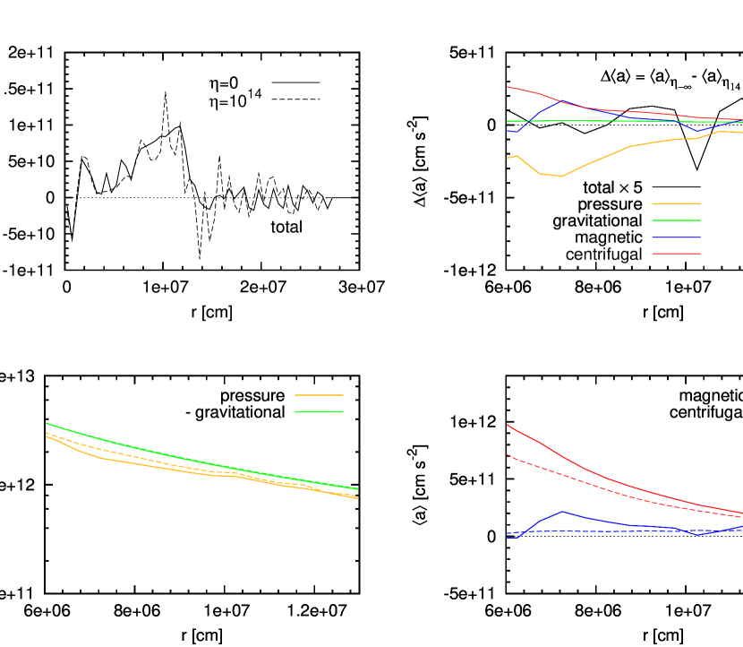
Figure 25.— Same as Fig. 7 but for model Bm-$\Omega$-$\eta_{-\infty}$ and Bm-$\Omega$-$\eta_{14}$. Radial accelerations are angularly averaged in the eruption-region and time averaged during $t=160-170$ ms. In the right-top panel the difference in the total acceleration is multiplied by 5.

-

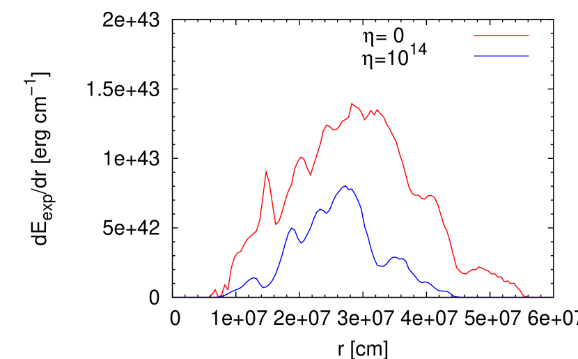
Figure 26.— Radial distributions of $dE_{\textrm{exp}}/dr$ at 170 ms in model Bm-$\Omega$-$\eta_{-\infty}$ and Bm-$\Omega$-$\eta_{14}$.

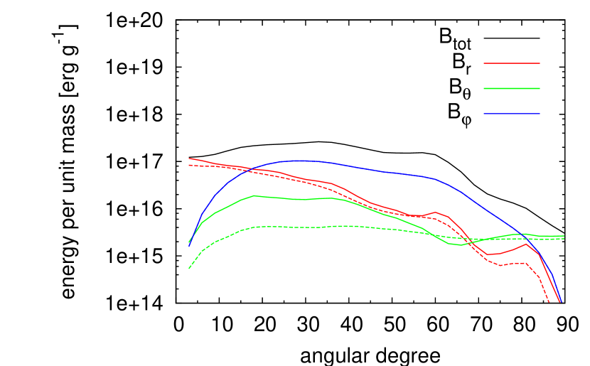
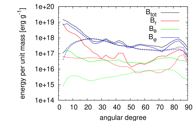
Figure 27.— Angular distributions of magnetic energies per unit mass averaged over $50$ km$<r<0.9\times r_{\textrm{sh}}$ at $t=143$ ms (2 ms after bounce; left) and $t=180$ ms (39 ms after bounce; right). The solid and dashed lines are for models Bm-$\Omega$-$\eta_{-\infty}$ and Bm-$\Omega$-$\eta_{14}$, respectively.

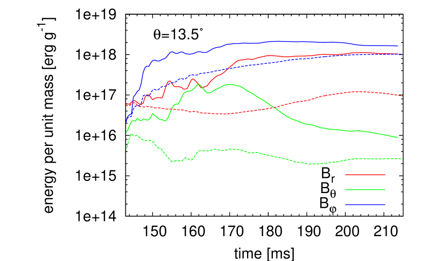
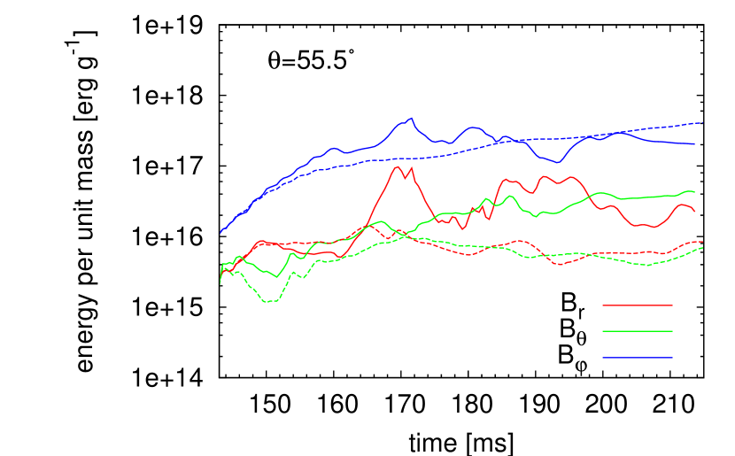
Figure 28.— Evolutions of the average magnetic energies per unit mass of volume $V_{13.5}$ (left) and $V_{55.5}$ (right). The solid lines are for model Bm-$\Omega$-$\eta_{-\infty}$ while the dashed lines are for Bm-$\Omega$-$\eta_{14}$. The graphs are plotted from $t=143$ ms (2 ms after bounce).

4.2.2 Magnetic Field Amplification

A magnetic field amplification in the present model-series goes on in a similar way as in the stronger magnetic field case Bs-$\Omega$. Fig. 27 shows the distributions of magnetic energies per unit mass, averaged over $50$ km$<r<0.9\times r_{\textrm{sh}}$ at $t=143$ ms (2 ms after bounce) and $t=180$ ms (39 ms after bounce), for model Bm-$\Omega$-$\eta_{-\infty}$ and Bm-$\Omega$-$\eta_{14}$. Again, it is observed that the contrast in a magnetic energy per unit mass over $\theta$ becomes stronger at the latter time. The evolutions of the magnetic energies per unit mass in two representative volumes $V_{13.5}$ and $V_{55.5}$ are shown in Fig. 28, which indicates that the difference between them becomes larger from 143 ms to 214 ms.

Here, we also evaluated each term in the evolution equations of magnetic energies per unit mass (see Eqs. (89) and (4.1.2)). The results are shown in Fig. 29 and 30. It is found both in model $\eta_{-\infty}$ and $\eta_{14}$ that the amplification mechanisms in volume $V_{13.5}$ are similar to those found in volume $V_{25.5}$ of model-series Bs-$\Omega$, i.e. the toroidal and radial magnetic energy are mainly amplified or kept due to an advection and shear (see § 4.1.2). As in the former model-series, we found here that the amplification is weaker in a volume with a lager $\theta_{\textrm{s}}$, viz. weaker in volume $V_{55.5}$.

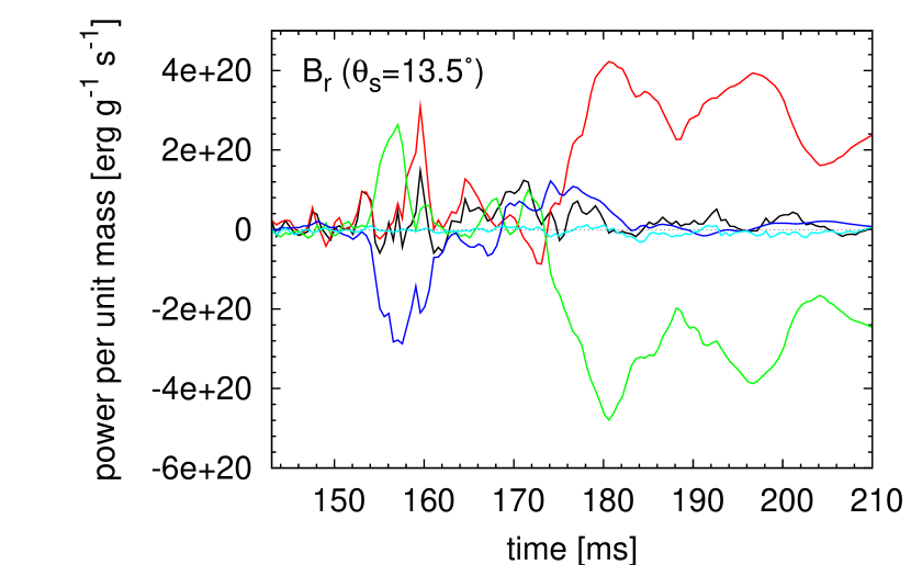
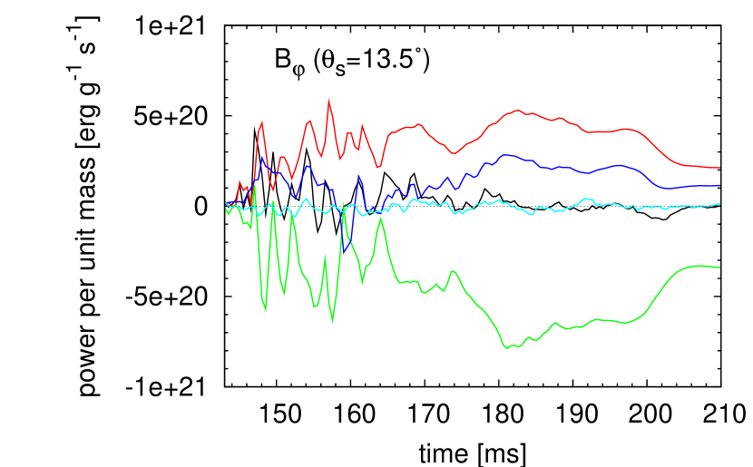
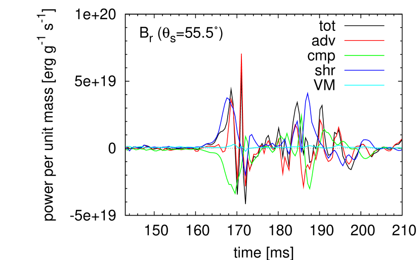
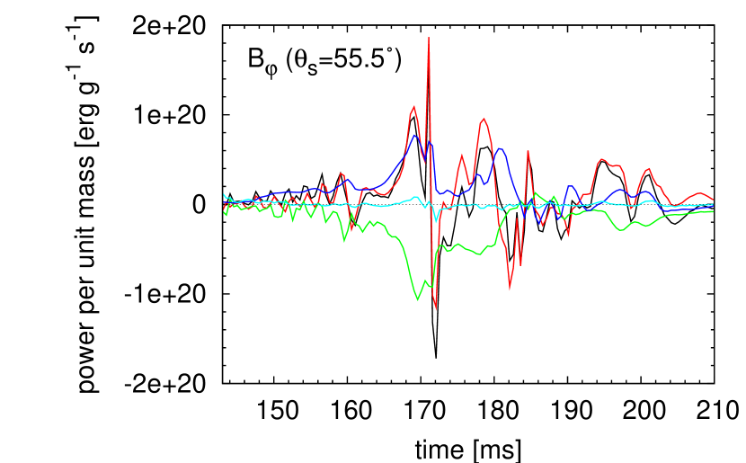
Figure 29.— Evolution of each $\dot{\mathscr{E}_{r}}$ and $\dot{\mathscr{E}_{\phi}}$ (see Eq. (4.1.2)) in a volume $V_{13.5}$ and $V_{55.5}$ in model Bm-$\Omega$-$\eta_{-\infty}$.

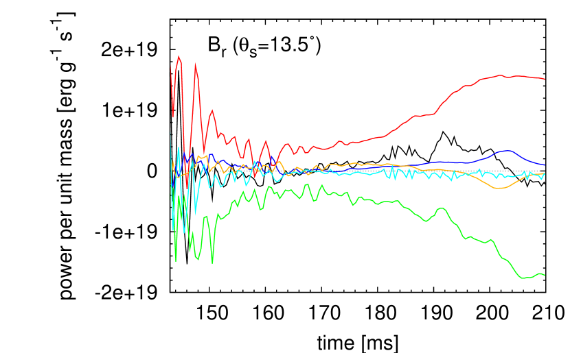
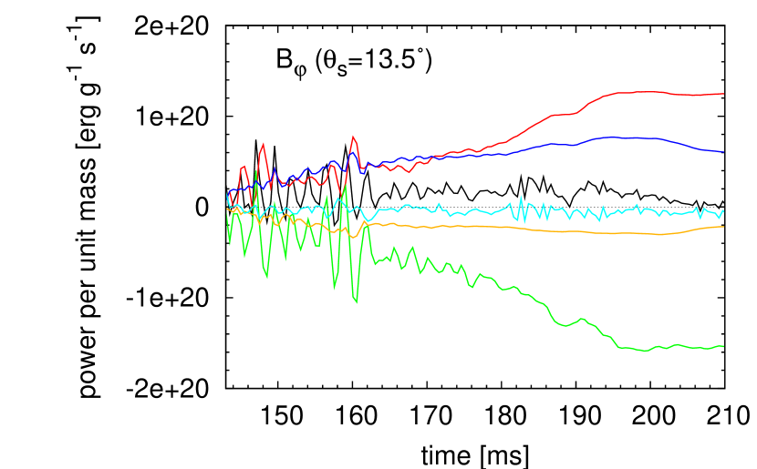
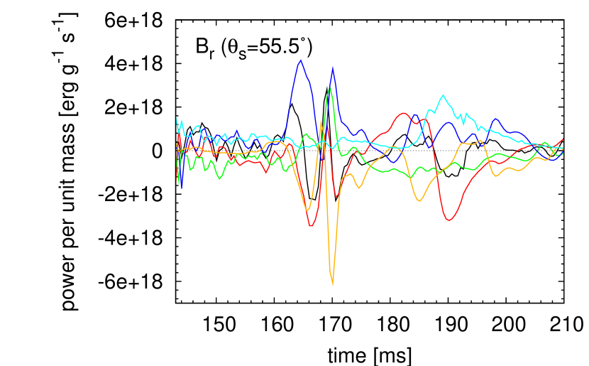
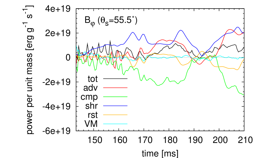
Figure 30.— Same as Fig. 29 but for model Bm-$\Omega$-$\eta_{14}$. Note that the vertical scale of each panel in Fig. 29 and 30 are different.

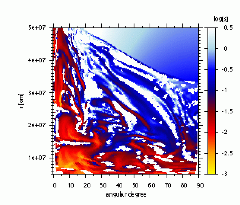
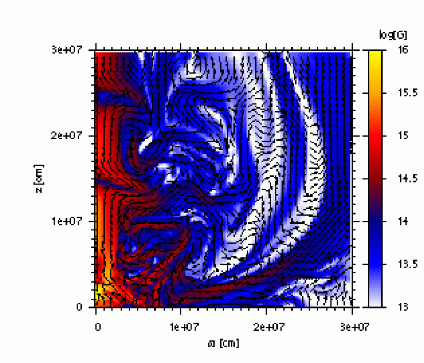
Figure 31.— Left-top panel: Distribution of MRI growth time in logarithmic scale in $\theta$-$r$ plane. White-colored regions include a location that is stable against the MRI. Right-top panel: Poloidal magnetic field vectors on top of a color map of poloidal magnetic field strength in logarithmic scale. Left-bottom panel: Distribution of fastest growing wave length, $\lambda^{*}\sim 2\pi c_{\textrm{A}}/\Omega$, where $c_{\textrm{A}}$ is the Alfvén velocity of a poloidal magnetic field. Right-bottom panel: Distribution of fastest growing wave length divided by numerical cell size, $\lambda^{*}/\sqrt{(\Delta x)^{2}+(\Delta z)^{2}}$. Yellow-colored region includes MRI-stable locations. These figures are depicted for model Bm-$\Omega$-$\eta_{-\infty}$ at $t=170$ ms.

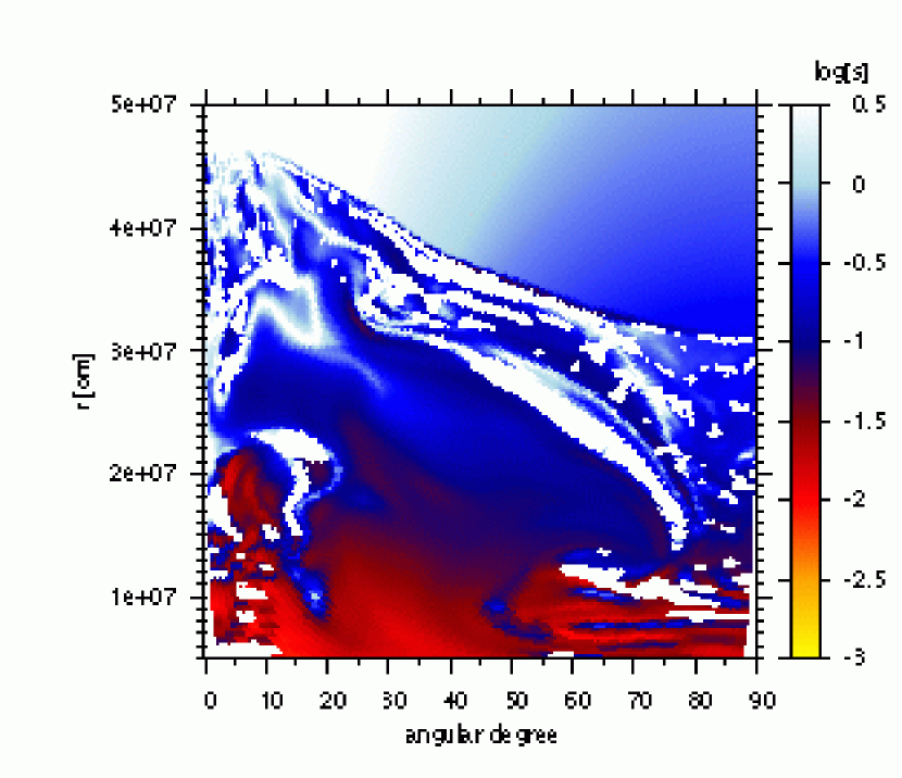
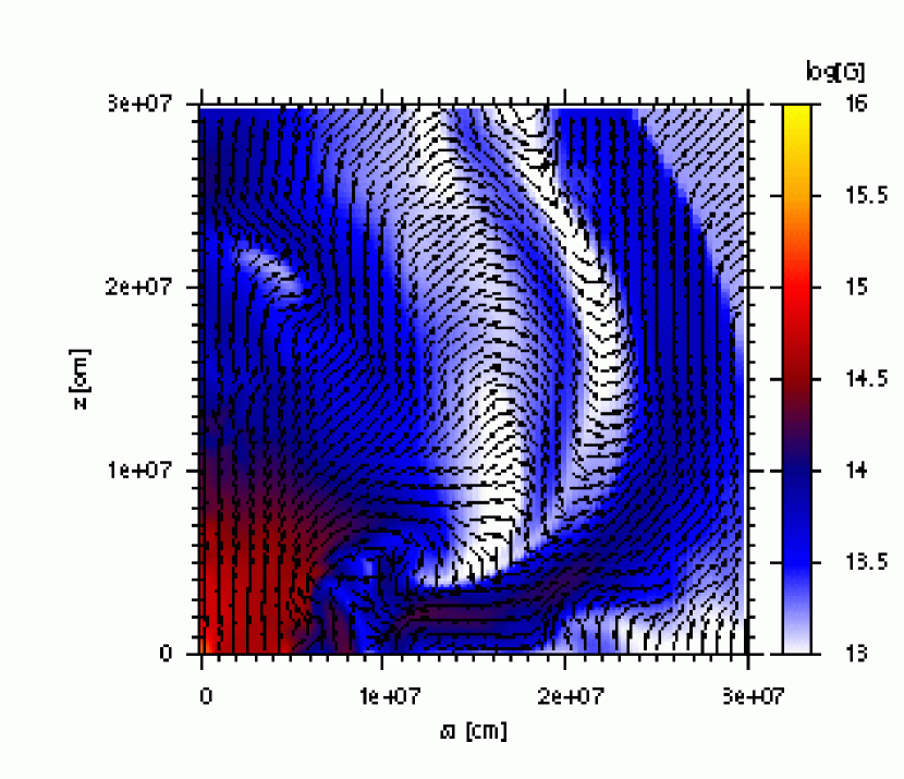
Figure 32.— Same as Fig. 31 but for model Bm-$\Omega$-$\eta_{14}$ at $t=170$ ms.

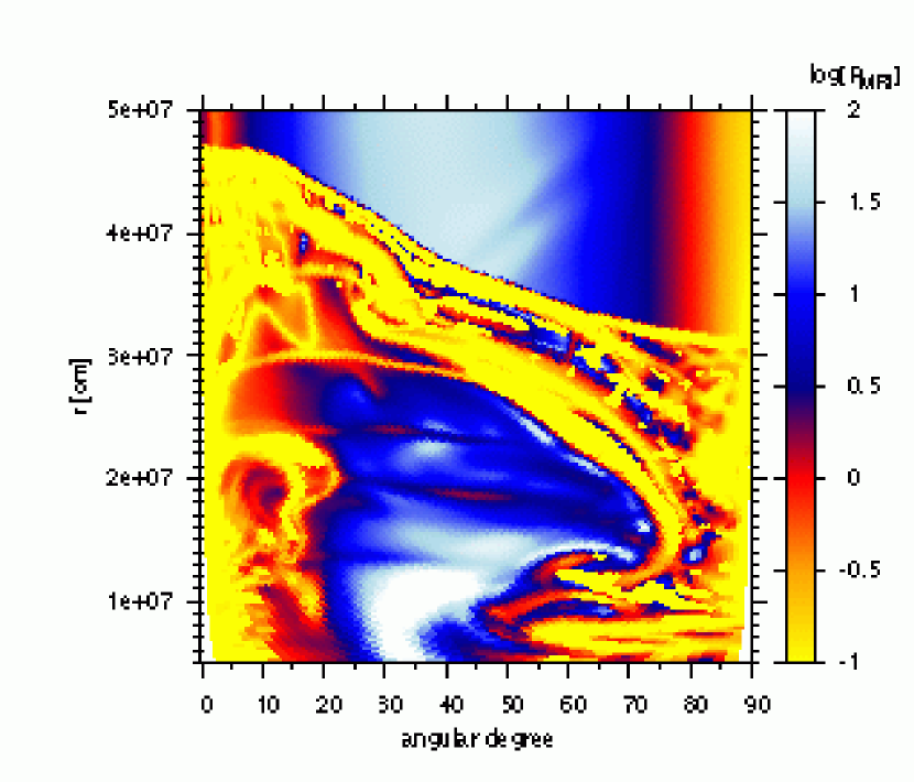
Figure 33.— Same as Fig. 18, but for model Bm-$\Omega$-$\eta_{14}$ at $t=170$ ms.

The left-top panel of Fig. 31 shows the distributions of MRI growth timescale in $\theta$-$r$ plane for model Bm-$\Omega$-$\eta_{-\infty}$ at $t=170$ ms (29 ms after bounce). It is found that a MRI growth timescale is short, $\sim$ a few ms to $10$ ms, in a considerable part for $r\lesssim 20^{\circ}$, while for a larger $\theta$, a growth timescale is averagely much longer. We found that a short growth timescale mentioned above is kept from 148 ms ($7$ ms after bounce) until the end of the simulation. In this model, the growth of MRI is also assured by magnetic field-line bending, which start appearing shortly after $150$ ms. The right-top panel of Fig. 31, which depicts the structure of poloidal magnetic field for $t=170$ ms, shows apparent field-line bending especially around the pole, where a growth timescale is averagely short.

In § 4.1.2, we have seen that in both model Bs-$\Omega$-$\eta_{-\infty}$ and Bs-$\Omega$-$\eta_{14}$, the shear term for volume $V_{25.5}$ starts increasing around the time when the growth of the MRI is expected, and thus we speculated that the increase is caused by the MRI. In the present model, Bm-$\Omega$-$\eta_{-\infty}$, the shear term for volume $V_{13.5}$ does not behaves like that. As seen in the left-top panel of Fig. 29, it has a large negative value around $\sim 155$-$160$ ms and a large positive value around $\sim 170$-$180$ ms. With this rather complicated behavior, it is difficult to guess when the MRI gives a substantial contribution to the shear term. Nonetheless, we could at least state that the MRI does not play a crucial role in amplifying a magnetic field. This is because the radial magnetic energy has already grown strong enough by the period of $\sim 170$-$180$ ms, while only during this period of time, the shear term works to amplify the magnetic field (see Fig. 28 and 29).

In model $\eta_{14}$, a region of short growth timescale is not as limited to a small $\theta$ as in model $\eta_{-\infty}$, albeit a growth timescale is averagely longer, typically a few 10 ms. As seen in the left-top panel of Fig. 32, although a small-$\theta$ region is more favorable site for the MRI, a large-$\theta$ region is still subjected to a fast MRI. However, as noted in § 4.1.2, we should take into account that the growth of MRI may be suppressed by resistivity. In Fig. 33, the distribution of $R_{\textit{MRI}}$, resistive timescale divided by MRI growth timescale, is depicted at $t=170$ ms for model $\eta_{14}$. It is shown that $R_{\textit{MRI}}$ is smaller than unity in the vicinity of the pole and equator, which means no growth of MRI there. We found that, for $20^{\circ}\lesssim\theta\lesssim 40^{\circ}$, $R_{\textit{MRI}}$ is always larger than unity in a considerable parts of the fast MRI regions. Hence, the MRI still seems to work also in model $\eta_{14}$. In the right-top panel of Fig. 32, MRI-like field-line bending is also found around the pole, albeit less prominent than in the ideal model.

In model $\eta_{14}$, the shear term for volume $V_{13.5}$ becomes large at late time, $\sim 190$ ms (the left-top panel of Fig. 30). Since, as well as in the former models, the radial magnetic energy does not largely increase after this time (the left panel of Fig. 28), the shear term and thus the MRI does not seem to very important for a amplification of a magnetic field, although they may play some role in keeping the strength of a magnetic field.

Compared with model-series Bs-$\Omega$, the computations of present model-series have poorer spatial resolution for capturing MRI (see the right-bottom panels of Fig. 31 and 32). Especially, in model Bm-$\Omega$-$\eta_{-\infty}$, the fastest growing wave length is resolved with less than 10 numerical cells in some locations even for $r>50$ km, where a magnetic field plays a dynamically important role. However, since these locations are limited to small areas, we do not expect that the dynamics would drastically change, if the growth of the MRI were fully resolved there.

Comparing the right panels of Fig. 12 and 27, the distribution of magnetic energy in model Bm-$\Omega$-$\eta_{-\infty}$ is more concentrated towards small $\theta$ than in model Bs-$\Omega$-$\eta_{-\infty}$. Although the two figures are depicted at different times, the above mentioned feature is still observed for the distributions compared at the same physical time after bounce (e.g. 37 ms after bounce for the both models). This may be explained as follows. Because a magnetic field of model Bm-$\Omega$-$\eta_{-\infty}$ is weaker, a strong matter eruption supported by magnetic force is restricted to a small region in the vicinity of the pole, where a magnetic field is relatively strong. Then due to an amplification of magnetic field by a radial advection, the contrast between a magnetic energy in the vicinity of the pole and the other region becomes stronger and stronger.

4.2.3 Aspect Ratio

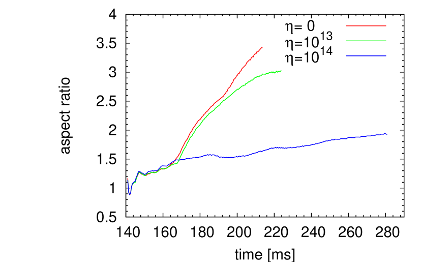
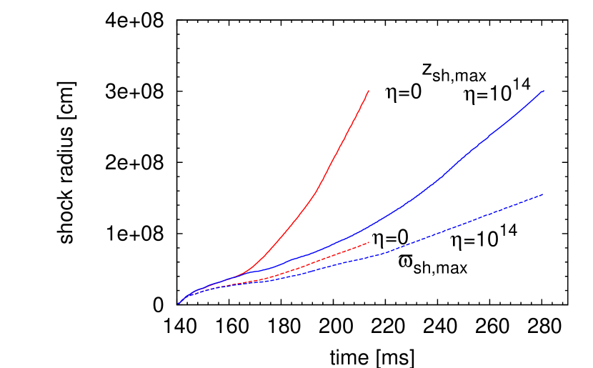
Figure 34.— Evolutions of aspect ratios (left panel) and the maximum ejecta positions in $z$ and $\varpi$ (right panel) in model series Bm-$\Omega$.

The aspect ratio of a shock surface is also become smaller for a larger resistivity in models-series Bm-$\Omega$ (see left panel of Fig. 34). As seen in right panel of Fig. 34, the difference in the aspect ratio is attained due to that in $z_{\textrm{ej,max}}$ as in the case of models-series Bs-$\Omega$. The same discussion as before will explain this feature, i.e. a stronger magnetic field and thus a larger magnetic and centrifugal acceleration in a small $\theta$ compared with in a large $\theta$ make a shock surface prolate, which is, however, less standout with the presence of a resistivity. A trait of the present model-series is a larger impact of resistivity, i.e. the aspect ratio is larger in model Bm-$\eta_{-\infty}$ than in model Bs-$\eta_{-\infty}$, while it is smaller in model Bm-$\eta_{14}$ than in model Bs-$\eta_{14}$.

The larger aspect ratio in model Bm-$\Omega$-$\eta_{-\infty}$ than in Bs-$\Omega$-$\eta_{-\infty}$ would be related to the distribution of the magnetic energy, which is more notably concentrated towards small $\theta$ in the former model, as discussed in § 4.2.2. The smaller aspect ratio in model Bm-$\Omega$-$\eta_{14}$ than in Bs-$\Omega$-$\eta_{14}$ may be understood as follows. Although the distributions of magnetic energy is similar in their shape between the two models (compare the right panels of Fig. 12 and 27), its magnitude is averagely weaker in model Bm-$\Omega$-$\eta_{14}$, reflecting the initial field strength, and a role of magnetic field in erupting matter is less important than in Bs-$\Omega$-$\eta_{14}$. As a result, the shape of a shock surface is not very much affected by magnetic field, and then the aspect ratio becomes smaller.

4.3. Very Strong Magnetic Field and No Rotation — Model Series Bss-$\mho$

The dynamical evolutions found in model-series Bss-$\mho$ are qualitatively different from those in the former two model-series. Without rotation, neither the generation of a toroidal magnetic field nor an angular momentum transfer occurs. However, a magnetic field still seems to play some role. The initially strong magnetic field affects the dynamics even during the collapse. A typical evolution proceeds as follows. Although a total magnetic energy per unit mass is a priori smaller around the equator, that of the $B_{\theta}$ is conversely larger there. A strong $B_{\theta}$ attenuates a matter infall around the equator, and leads to a weak bounce in the lateral direction. Due to the weak bounce, outgoing matters are soon prevailed by falling matters, and then the infall-region forms around the equator. Meanwhile, in the other part, a bounce occurs strong enough to form the eruption-region, and with a help of a magnetic force, especially a magnetic pressure of $B_{\theta}$, the shock surface propagates outwards to reach 3000 km at the end of the simulation. Fig. 35 shows the distributions of velocity and magnetic field in model Bss-$\mho$-$\eta_{-\infty}$ and Bss-$\mho$-$\eta_{14}$ at $t=195$ ms (40 ms after bounce). In each of the left panels, the formation of the eruption-region and infall-region is well observed. Each right panel shows that a magnetic pressure is mildly important in the eruption-region. As shown in Fig. 36 the magnetic energies in the two models are $\sim 10^{51}$ erg. This implies that a magnetic field has a potential to somewhat boost the explosion. Although no significant difference between model $\eta_{-\infty}$ and $\eta_{14}$ can be found in Fig. 35, as we will see soon later, a resistivity still plays a certain role in the dynamics of the present model-series.

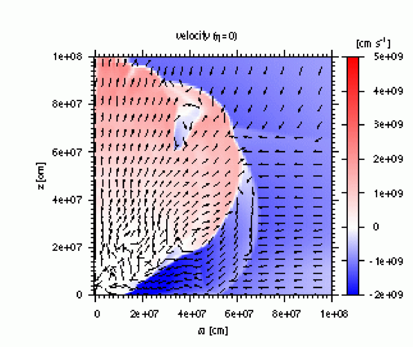
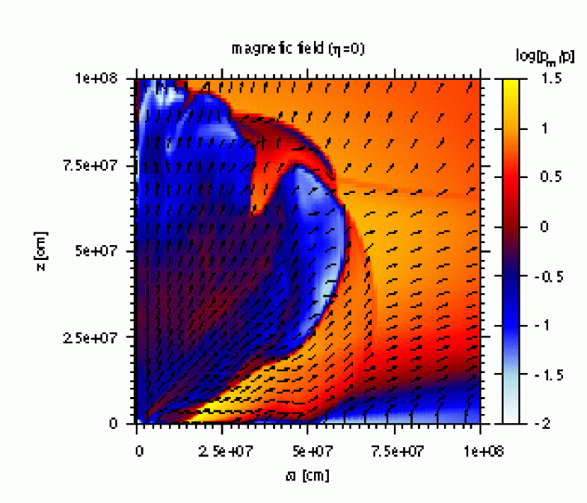
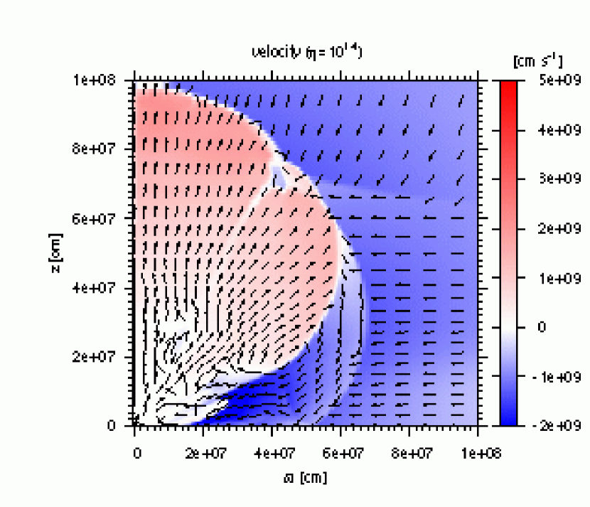
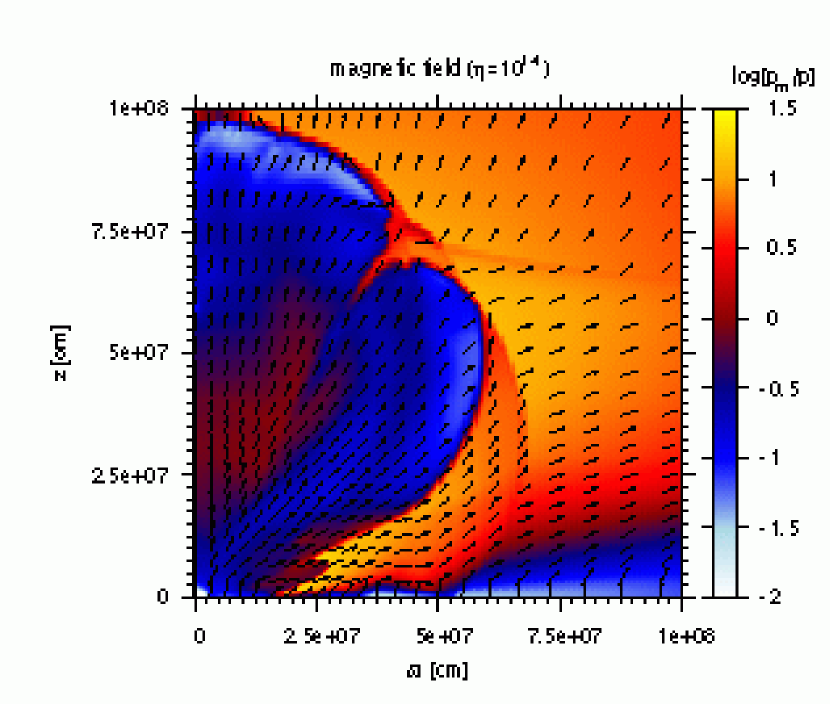
Figure 35.— Same as Fig. 5 but for model Bss-$\mho$-$\eta_{-\infty}$ (upper panels) and Bss-$\mho$-$\eta_{14}$ (lower panels) depicted at $t=195$ ms.

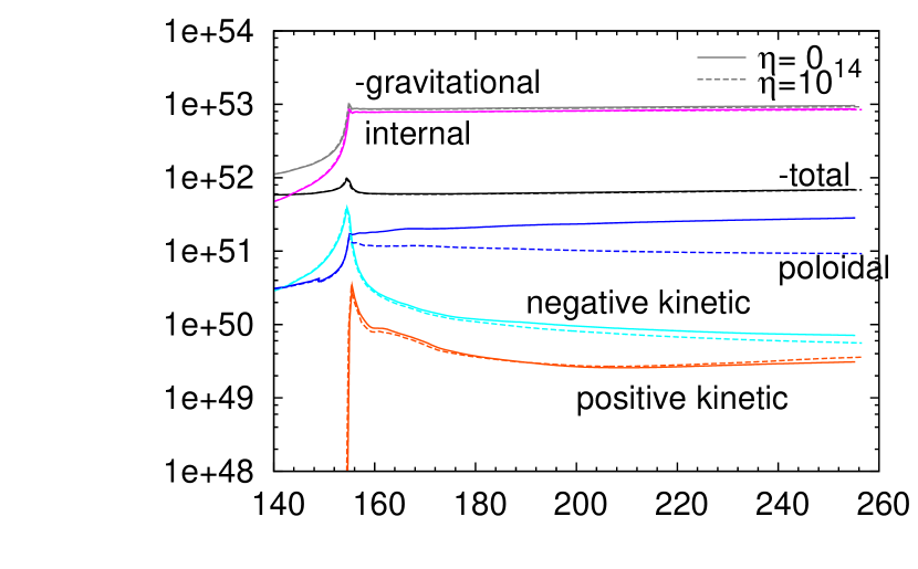
Figure 36.— Evolutions of the total (black lines), internal (magenta), gravitational (gray), positive kinetic (orange), negative kinetic (cyan), and poloidal magnetic (blue) energy integrated over the whole numerical domain. The total and gravitational energy are multiplied by $-1$. The solid and dashed lines are drawn for model Bss-$\mho$-$\eta_{-\infty}$ and Bss-$\mho$-$\eta_{14}$, respectively.

4.3.1 Explosion Energy and Diffusion of Magnetic Field

In Fig. 37, the evolution of explosion energies in model-series Bss-$\mho$ are plotted. As shown there, the explosion energies are found to be $\sim 10^{50}$ erg, one order of magnitude smaller than that of a canonical supernova. The figure also indicates that the models involving resistivity produce a larger explosion energy compared with the ideal model, which is opposite to what is found in the model-serieses involving rotation.

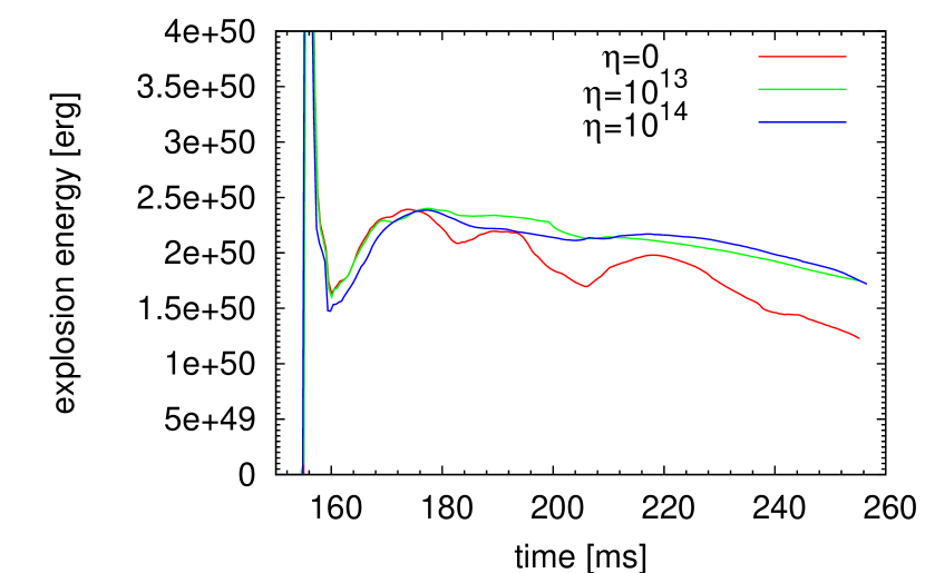
Figure 37.— Evolutions of explosion energies in model-series Bss-$\mho$.

In Fig. 38, we plot the radial distributions of $dE_{\textrm{exp}}/dr$ at $t=201$ ms in model Bss-$\mho$-$\eta_{-\infty}$ and Bss-$\mho$-$\eta_{14}$, which shows that the explosion energy in model $\eta_{14}$ is grater than that in model $\eta_{-\infty}$ at most radial range. We examined whether a radial acceleration in model $\eta_{14}$ is lager than in model $\eta_{-\infty}$, but found no substantial difference between them. We also compared the two models by the radial distributions of radial velocity angularly averaged in the eruption-region at 201 ms (see Fig. 39). It is found that a radial velocity is mostly larger in model $\eta_{14}$. This seems a key factor to know why the explosion energy is larger in model $\eta_{14}$.

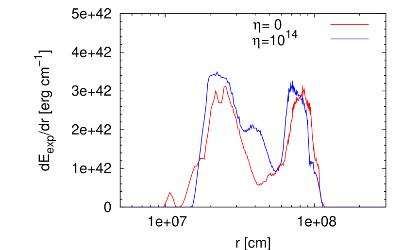
Figure 38.— Radial distributions of $dE_{\textrm{exp}}/dr$ at $t=201$ ms in model Bss-$\mho$-$\eta_{-\infty}$ and Bss-$\mho$-$\eta_{14}$.

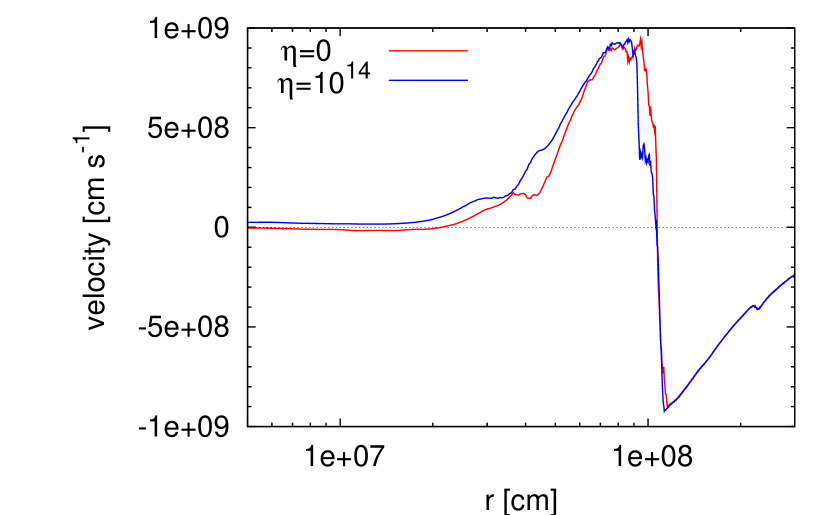
Figure 39.— Radial distributions of radial velocities angularly averaged in the eruption-region, at $t=201$ ms in model Bss-$\mho$-$\eta_{-\infty}$ and Bss-$\mho$-$\eta_{14}$.

Then a question is why a radial velocity is larger in model $\eta_{14}$, despite comparable strengths of radial accelerations. In Fig. 40, the velocity distributions in $\varpi$-$z$ plane at $t=201$ ms are depicted for the two models with a little zooming towards the center. For model $\eta_{-\infty}$, it is observed that matters flow from the infall-region into the eruption-region around $r\lesssim 200$ km, and there damps a matter ejection. In model $\eta_{14}$, on the other hand, a matter flow into the eruption region is inhibited by a ”positive velocity island” observed around 150 km $\lesssim r\lesssim$ 350 km in the infall-region, and a coherent outflow of matter in the eruption-region is well kept even for $r\lesssim 200$ km. In this way, the appearance of the positive velocity island seems to be related to the difference in the velocity distribution observed between the two models.

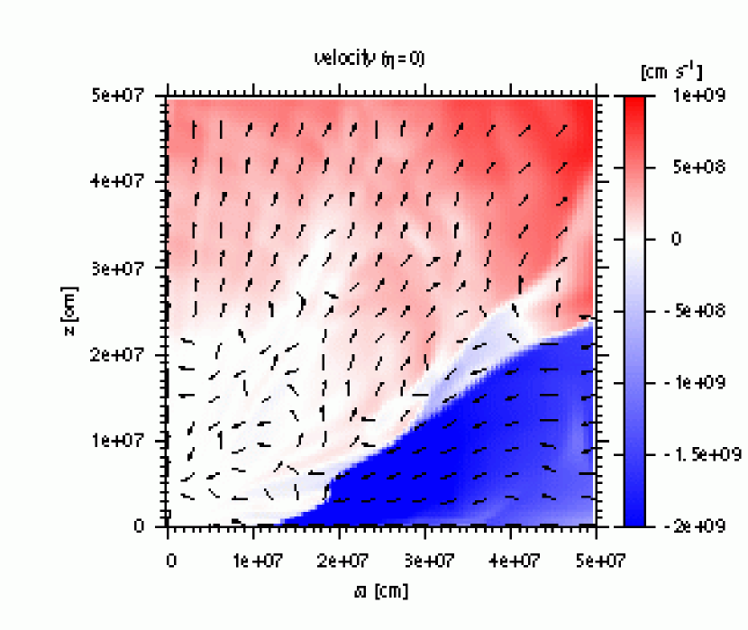
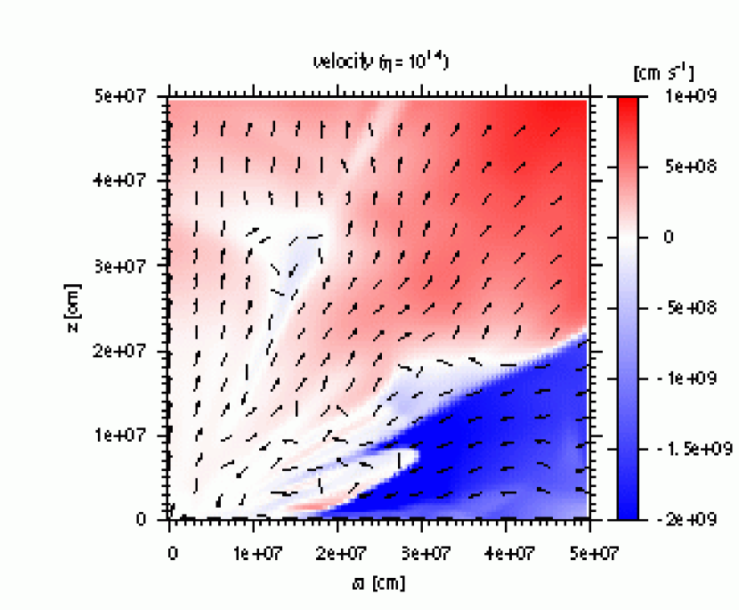
Figure 40.— Distributions of radial velocity magnitude (color) and velocity directions (vectors) at $t=201$ ms for models Bss-$\mho$-$\eta_{-\infty}$ (left) and Bss-$\mho$-$\eta_{14}$ (right).

We found that the positive velocity island begins to emerge around $170$ ms (15 ms after bounce) in model $\eta_{14}$. Fig. 41 shows the radial distributions of radial velocities, angularly averaged in the infall-region at 175 ms, for the two models. It is observed in the radial range of 60 km$\lesssim r\lesssim$180 km that a infall velocity is slower in model $\eta_{14}$, which seems due to the positive velocity island. In Fig. 42, the radial distributions of radial accelerations, angularly averaged in the infall-region and time averaged during $t=170$-$175$ ms, is plotted. As expected, a radial acceleration in the infall-region is larger in model $\eta_{14}$ around a similar radial range to the above, 90 km$\lesssim r\lesssim$180 km. We found that a larger pressure and magnetic acceleration are responsible for this acceleration superiority (see right panel of Fig. 42). We speculate that a larger pressure acceleration in model $\eta_{14}$ will not be caused by the Joule heating, since the heating timescale in the above range is too long, $\sim$1-10 s, to produce an extra pressure. It is more likely that the accumulation of falling matter stemmed by magnetic acceleration makes a pressure in the positive velocity island larger. It seems that a magnetic acceleration is the primary factor for the formation of the positive velocity island.

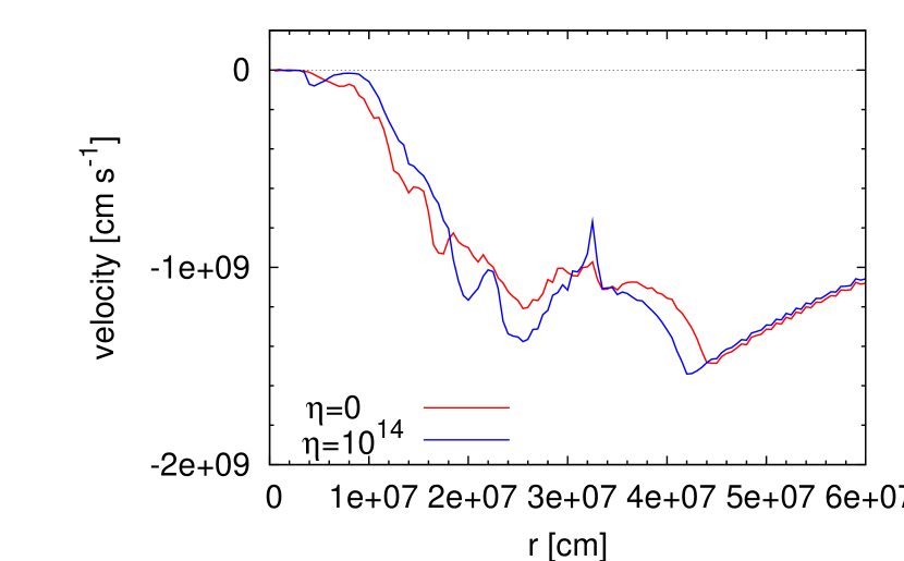
Figure 41.— Radial distributions of average velocities in the infall-region at $t=175$ ms in models Bss-$\mho$-$\eta_{-\infty}$ and Bss-$\mho$-$\eta_{14}$.

Figure 42.— Left: Radial distributions of radial acceleration, $\langle a\rangle$, angularly averaged in the infall-region and time averaged during $t=170-175$ ms, for Bss-$\mho$-$\eta_{-\infty}$ and Bss-$\mho$-$\eta_{14}$. Right: The radial distributions of differences in the averaged radial accelerations, $\Delta\langle a\rangle\equiv\langle a\rangle_{\eta_{-\infty}}-\langle a\rangle_{\eta_{14}}$, subtracting that of model $\eta_{14}$ from that of model $\eta_{-\infty}$.

In the absence of toroidal magnetic field, a radial magnetic acceleration is written as

$$a_{\textrm{B}}=\frac{B_{\theta}}{\rho}\left(-\frac{\partial B_{\theta}}{\partial r}+\frac{1}{r}\frac{\partial B_{r}}{\partial\theta}-\frac{B_{\theta}}{r}\right).$$ (91)

The radial distributions of magnetic field in the infall-regions at 175 ms plotted in the left panel of Fig. 43 indicates that $B_{r}$ is far grater than $B_{\theta}$ in the above radial range of 90-180 km, and thus the second term in r.h.s. of Eq. (91), a part of magnetic tension, is dominant. The left panel of Fig. 43 also shows that, in the above radial range, $B_{\theta}$ is larger in model $\eta_{14}$ than in model $\eta_{-\infty}$, while $B_{r}$ is smaller in model $\eta_{14}$. We found that the superiority in $B_{\theta}$ overwhelms the inferiority in $B_{r}$ , i.e. $B_{r}(r)B_{\theta}(r)$ is averagely larger in model $\eta_{14}$ in the above radial range. To put it simply, a larger $B_{\theta}$ in in model $\eta_{14}$ is crucial to the formation of the positive velocity island.

The radial distribution of $B_{\theta}$ in model $\eta_{14}$ shown in the left panel of Fig. 43 compared with that of model $\eta_{-\infty}$ invokes a magnetic field diffusion. Indeed, it is found that a magnetic Reynolds number is smaller than unity almost everywhere for $r\lesssim 85$ km in the infall-region (see the right panel of Fig. 44), viz. a diffusion effectively advects a magnetic field outwards against matter infall. The right panel of Fig. 43 shows that $B_{\theta}$ in model $\eta_{-\infty}$ is highly confined into the central region of 30 km radius, while the $B_{\theta}$-distribution in model $\eta_{14}$ is rather gentle. This implies that in the latter model, a resistivity effectively diffuses $B_{\theta}$ out of the central region. In model $\eta_{-\infty}$, the gradient of $B_{\theta}$ suddenly becomes shallow around $r=30$ km. Then with a resistivity, the incoming diffusion flux there, $\eta\nabla B_{\theta}$, would be larger than the outgoing one, which would result in a increase of $B_{\theta}$ outside the radius of 30 km. In this way, a magnetic field diffused out from a deep inside of the core suppress a matter infall and responsible for a larger explosion energy in model $\eta_{14}$.

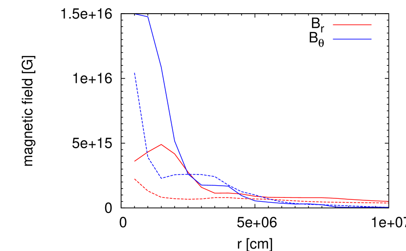
Figure 43.— Left: The radial distributions of magnetic field strengths in the infall-regions at $t=175$ ms in model Bss-$\mho$-$\eta_{-\infty}$ (solid lines) and Bss-$\mho$-$\eta_{14}$ (dashed lines). Right: Same as the left panel but in linear scale, zooming towards the center.

A similar mechanism also works in model $\eta_{13}$. As shown in the left panel of Fig. 44, diffusion of magnetic field in the infall-region also occurs well in this model. However, due to a smaller resistivity, diffusion sites are limited to a smaller volume compared with model $\eta_{14}$. Nonetheless, the explosion energy in model $\eta_{13}$ is comparable to that of model $\eta_{14}$ at the end of the simulations (see Fig. 37)

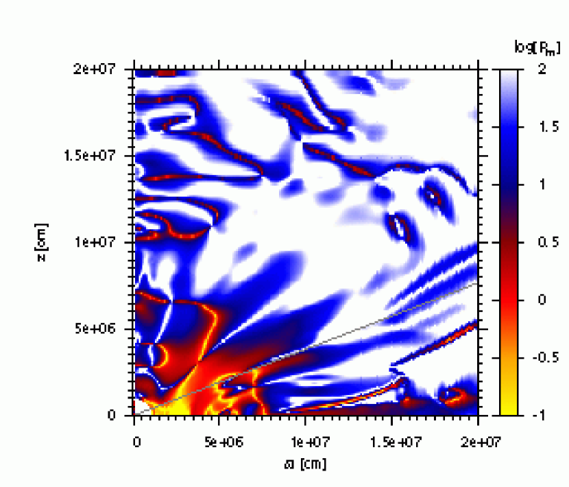
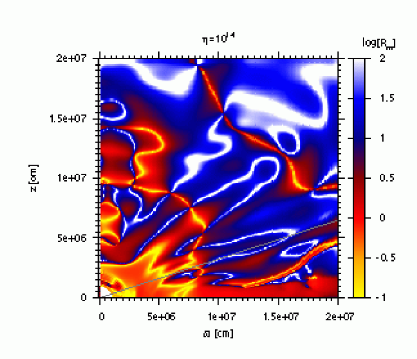
Figure 44.— Distributions of magnetic Reynolds number in logarithmic scale at $t=175$ ms in model Bss-$\mho$-$\eta_{13}$ (left) and Bss-$\mho$-$\eta_{14}$ (right). The volume below the gray line corresponds to the infall region.

4.3.2 Aspect Ratio

The aspect ratios in model-series Bss-$\mho$ are also larger than unity, i.e. the shape of ejecta is prolate, but are not as large as in the rotating cases (see Fig. 45). Since the initial magnetic field assumed in the present model-series is very strong, it affects the dynamics even before bounce. Due to the dipole-like configuration, a magnetic field hampers a matter infall especially well in the lateral direction. This causes a weak bounce around the equator, and thus a prolate matter ejection.

The difference from the former model-series is that the aspect ratios do not grow drastically after bounce (see Fig. 45). We expect that this is caused by a roughly flat angular distribution of magnetic energy per unit mass in the eruption-region as indicated in Fig. 46 for model Bss-$\mho$-$\eta_{-\infty}$ and Bss-$\mho$-$\eta_{14}$, reminding that a polarly concentrated magnetic field distribution is essential for a large aspect ratio in the rotating cases.

We found that the change from the rather polarly concentrated distribution of magnetic field at the beginning to a roughly flat angular distribution occurs during the collapsing phase, i.e. before bounce. Fig. 47 shows the angular distributions of $\dot{\mathscr{E}_{r}}$, radially averaged over $50<r<1000$ km at 122 ms (33 ms before bounce) in model Bss-$\mho$-$\eta_{-\infty}$. It is shown that a total $\dot{\mathscr{E}_{r}}$ is larger around the equator, and a compression of $B_{r}$ in the $\theta$-direction plays an important role. Since $B_{\theta}$ is a priori strong around the equator due to the assumed magnetic field configuration, an infall matter there is a little deflected into non-radial direction by a Maxwell stress of $B_{r}B_{\theta}/4\pi$, viz. $\theta$-component of velocity is generated. In this way, $B_{r}$ is compressed into the $\theta$-direction, which leads to an increase of $B_{r}$ preferentially around the equator and rather flat angular distribution of magnetic field.

A notable point here is that a rather flat distribution of magnetic field, which causes a mild value of the aspect ratio, is established before bounce when a resistivity does not work well because of a large scale height of magnetic field. This is why the aspect ratio for a different resistivity results in a similar value.

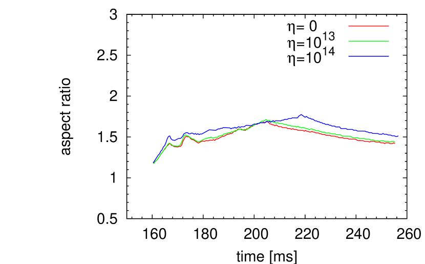
Figure 45.— Evolutions of aspect ratios in model series Bss-$\mho$.

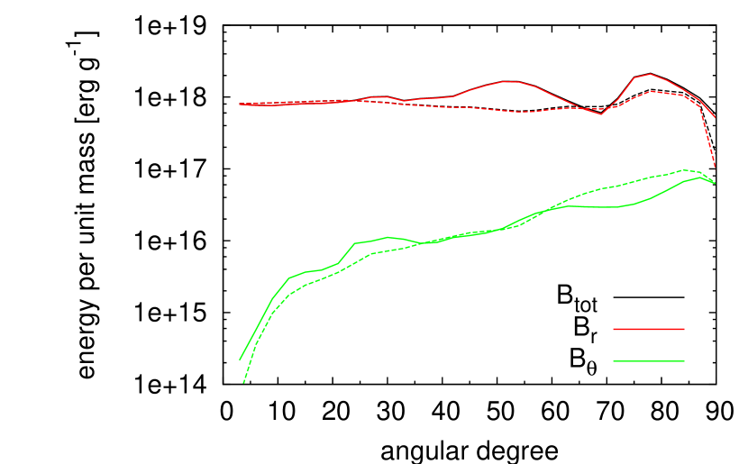
Figure 46.— Angular distributions of magnetic energies per unit mass averaged over $50$ km$<r<0.9\times r_{\textrm{sh}}$ at $t=180$ ms (25 ms after bounce). The solid and dashed lines are for models Bss-$\mho$-$\eta_{-\infty}$ and Bss-$\mho$-$\eta_{14}$, respectively.

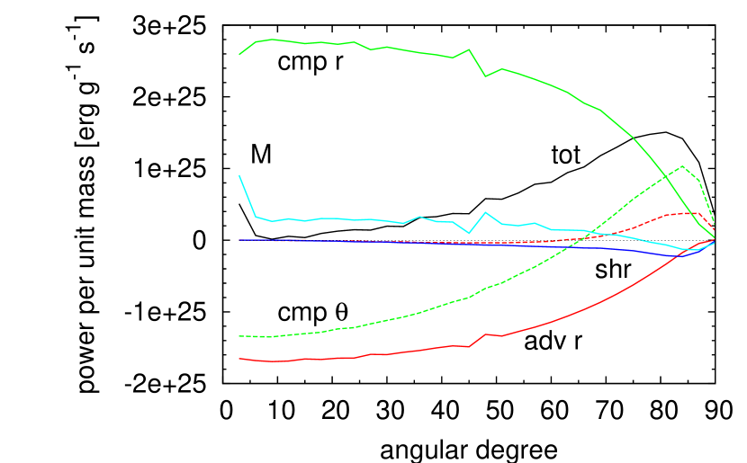
Figure 47.— Angular distributions of $\dot{\mathscr{E}_{r}}$, radially averaged over $50<r<1000$ km (see Eq. (4.1.2)) at 122 ms (33 ms before bounce) in model Bss-$\mho$-$\eta_{-\infty}$. The black line shows total $\dot{\mathscr{E}_{r}}$, while the red-solid, red-dashed, green-solid, green-dashed, blue, and cyan lines represent the contribution to $\dot{\mathscr{E}_{r}}$ from the radial advection, angular advection, radial compression, angular compression, shear, and change in mass, respectively.

4.4. Numerical Resistivity

In the preceding sections, we have seen how a resistivity impacts on the dynamics of a strongly magnetized supernova. However, we should remember that the numerical results are not only affected by a physical resistivity but may also be influenced by a numerical resistivity. Here, we estimate a possible impact of a numerical resistivity on the dynamics.

First, we directly compared the strengths of a physical resistivity and a numerical resistivity. We consider dividing a numerical flux into two terms, the advection term and numerical diffusion term, where the former may account for an advection of a physical flux, while the latter for a numerical diffusion. For example, in the equation of numerical fluxes $\mbox{{\boldmath$F$}}^{x}$ in Eqs. (LABEL:eq.kt.numfluxf), the first and second term in r.h.s. are the advection term and numerical diffusion term, respectively. Accordingly, the ideal part of a numerical flux vector for the induction equations $\bar{F}$, which are defined by a combinations of 6th - 8th components of numerical flux vectors $\mbox{{\boldmath$F$}}^{x}$ an $\mbox{{\boldmath$F$}}^{y}$ (see Eqs. (76)), are also divided into the advection term and numerical diffusion term. Then, the total numerical flux vector for the induction equations can be written as $\mbox{{\boldmath$\bar{E}$}}=\mbox{{\boldmath$\bar{F}$}}_{\textrm{adv}}+\mbox{{\boldmath$\bar{F}$}}_{\textrm{nd}}+\mbox{{\boldmath$\bar{G}$}}$, where subscripts ”adv” and ”nd” stand for advection and numerical diffusion, respectively. Recall that a term $\bar{G}$ arises due to a physical resistivity.

Now, to compare the strengths of a physical resistivity and a numerical resistivity we evaluate $\zeta\equiv|\mbox{{\boldmath$\bar{G}$}}|/|\mbox{{\boldmath$\bar{F}$}}_{\textrm{nd}}|$, in which a physical resistivity is dominant for $\zeta\gg 1$ while a numerical resistivity is dominant for $\zeta\ll 1$. The distribution of $\zeta$ for model Bs-$\Omega$-$\eta_{13}$ at 164 ms is shown in Fig. 48. This implies that a physical resistivity dominates over a numerical resistivity in a considerable volume inside the shock surface, but in some locations a numerical resistivity is not negligible.

Next, we examined how much a numerical resistivity affects the dynamics. This is done by evaluating $R_{\textrm{m,num}}\equiv|\mbox{{\boldmath$\bar{F}$}}_{\textrm{adv}}|/|\mbox{{\boldmath$\bar{F}$}}_{\textrm{nd}}|$, which may corresponds to a magnetic Reynolds number for a numerical resistivity. Even if a numerical resistivity dominates over a physical resistivity, it does not make substantial impacts on the dynamics provided $R_{\textrm{m,num}}\gg 1$. Fig. 49 shows the distribution of $R_{\textrm{m,num}}$ for model Bs-$\Omega$-$\eta_{13}$ at 164 ms. It is found that $R_{\textrm{m,num}}$ is much larger than unity almost everywhere except around the shock surface, where a steep variation of a magnetic field exists. Meanwhile, we have seen in § 4.1.4 that a magnetic Reynolds number of physical resistivity in model Bs-$\Omega$-$\eta_{13}$ is $\sim 30$ around the equator (see the left panel of Fig. 22). These facts imply that a numerical resistivity is mostly too small to influences the dynamics, while a physical resistivity affects the dynamics, albeit a little. Thus, it seems that a physical resistivity “effectively” dominates over a numerical resistivity in this model.

From the above discussion, it is likely that a comparison between $R_{\textrm{m}}$ and $R_{\textrm{m,num}}$ is more meaningful than that between a physical resistivity and numerical resistivity themselves in order to assess an influence of a numerical resistivity. Then, we also compare $R_{\textrm{m}}$ and $R_{\textrm{m,num}}$ for model Bm-$\Omega$-$\eta_{13}$ and Bss-$\mho$-$\eta_{13}$. In model Bm-$\Omega$-$\eta_{13}$, $R_{\textrm{m,num}}$ is much larger than unity almost everywhere except around the shock surface, while a relatively small $R_{\textrm{m}}\sim 1$-10 is found around the equator (see Fig. 50). Hence, a physical resistivity also effectively dominates over a numerical resistivity in this model. In model Bss-$\mho$-$\eta_{13}$, a mildly small $R_{\textrm{m,num}}\sim 10$ appears not only around the shock surface but also other locations (see the left panel of Fig. 51). This means that a numerical resistivity somewhat affects the dynamics in this model. However, the right panel of Fig. 51 shows that a physical resistivity is more influential than a numerical resistivity especially at small radii. Recalling that the essential role of a resistivity in this model is to diffuse a magnetic field from a small radius to a larger radius, a physical resistivity seems to play primary role to yield a different result for Bss-$\mho$-$\eta_{13}$ from the ideal model. For confirmation, we carried out the above analysis in the models with $\eta=10^{14}$ cm²s^-1, and found that the “effective” dominance of a physical resistivity over a numerical resistivity is more pronounced than the counterpart models with $\eta=10^{13}$ cm²s^-1.

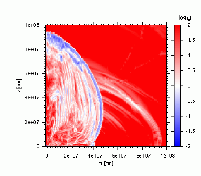
Figure 48.— Distribution of $\zeta\equiv|\mbox{{\boldmath$\bar{G}$}}/\mbox{{\boldmath$\bar{F}$}}_{\textrm{nd}}|$ in logarithmic scale for model Bs-$\Omega$-$\eta_{13}$ at 164 ms.

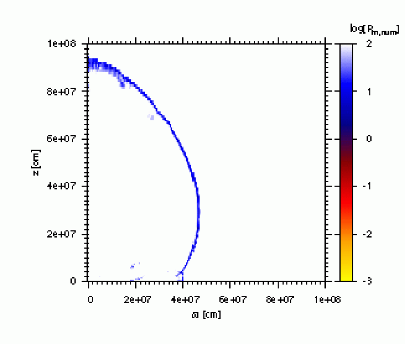
Figure 49.— Distribution of $R_{\textrm{m,num}}\equiv|\mbox{{\boldmath$\bar{F}$}}_{\textrm{adv}}|/|\mbox{{\boldmath$\bar{F}$}}_{\textrm{nd}}|$ in logarithmic scale for model Bs-$\Omega$-$\eta_{13}$ at 164 ms.

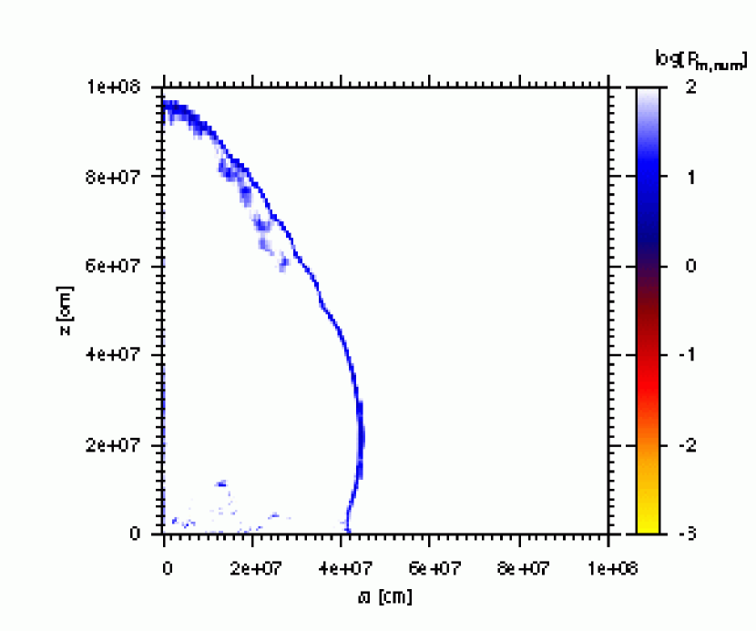
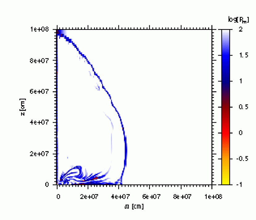
Figure 50.— Distribution of $R_{\textrm{m,num}}$ (left) and $R_{\textrm{m}}$ (right) in logarithmic scale for model Bm-$\Omega$-$\eta_{13}$ at 182 ms.

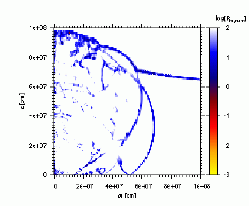
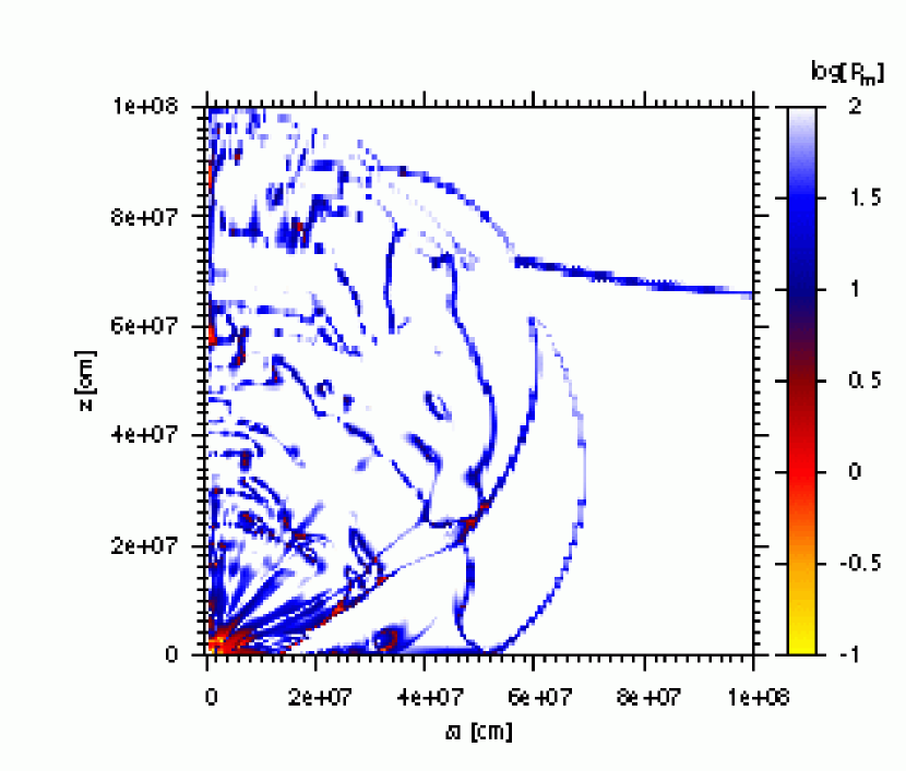
Figure 51.— Distribution of $R_{\textrm{m,num}}$ (left) and $R_{\textrm{m}}$ (right) in logarithmic scale for model Bss-$\mho$-$\eta_{13}$ at 195 ms.

5. Discussion and Conclusion

We have done MHD simulations of CCSNe to understand roles of a turbulent resistivity in the dynamics. As a result, we found that a resistivity possibly has a great impact on the explosion energy, a magnetic field amplification, and the aspect ratio. How and how much a resistivity affects on these depend on the initial strengths of magnetic field and rotation together with the strength of a resistivity.

In the rotating cases (model-series Bs-$\Omega$ and Bm-$\Omega$), a resistivity makes the explosion energy small. This is mainly ascribed to a small magnetic and centrifugal acceleration due to an inefficiency in magnetic field amplification and angular momentum transfer, respectively. Meanwhile, in the case of very strong magnetic field and no rotation (model-series Bss-$\mho$), a resistivity enhances the explosion energy. In the ideal model, an inflow of negative radial momenta from the infall-region into the eruption-region inhibits a powerful mass eruption. With a resistivity, a magnetic field in the infall-region diffuses outwards from a deep inside of the core to counteract the negative momentum invasion.

The ideal models involving rotation shows a polarly concentrated distribution of magnetic energy per unit mass. Since an initial magnetic energy per unit mass is somewhat larger around the pole than the equator, an amplification preferentially occurs there, which makes the contrast stronger. We found that the main mechanisms of amplification around the pole is an outward advection of a magnetic energy from a small radius and the winding of poloidal magnetic field-lines by differential rotation. In a resistive model, an amplification occurs qualitatively similar way to the corresponding ideal model, but proceeds less efficiently. As a result, the angular distribution of magnetic field becomes less concentrated towards the pole. Although we found signs of a MRI growth in these models, it seems not to play substantial role in amplifying a magnetic field. The MRI will at best help to keep the strength of a magnetic field. We should note here that in our 2D-axisymmetric simulations, the MRI may not be followed correctly, since non-axisymmetric modes are also important in the MRI. A comparison between a 2D-axisymmetric and 3D simulations in the behavior of the MRI will be made and presented elsewhere in the near future.

Every model involving a rotation shows a large aspect ratio, $>2.5$, at the end of the simulation, where a model with a larger resistivity results in a smaller aspect ratio. The impact of resistivity on the aspect ratio is more standout in the moderate magnetic field case, model-series Bm-$\Omega$. The aspect ratios obtained in the rotation models are expected to grow even larger later on, since a radial velocity is still faster around the pole than around the equator at the end of the simulations. Further long time computations are necessary to predict the aspect ratio after the shock surface breaks out the stellar surface. In a model without rotation, on the other hand, the aspect ratio keeps mild value, $\sim 1.5$, through each simulation. No significant difference is found among models with a different resistivity. It is found that the aspect ratios attained in the present simulations are related to the angular distribution of magnetic energy per unit mass. That is, the more a magnetic energy is concentrated towards a small $\theta$, the larger the aspect ratio of ejected matters.

In literature, we have found eight CCSNe in that both the upper and lower limit of the aspect ratio is measured; SN1987a, SN1993J, SN1997X, SN1998S, SN2002ap, SN2005bf, SN2007gr, and SN2010jl. The observed aspect ratios are at most $\approx 3$; e.g. $\approx 2-3$ for SN1987A (Papaliolios et al., 1989), $\approx 3$ for 1997X and $1.2-2.5$ for SN1998S (Wang et al., 2001). It seems that aspect ratios obtained in our rotational models are too large compared with these observations, reminding that ours will grow larger later on. However, we note that the above sample does not necessarily contain supernovae that leave a magnetar. Applying SGR/AXP birth rate of $\sim 0.1-0.2$ per century (Leahy & Ouyed, 2007) and Galactic CCSN rate of $\sim 0.8-3.0$ per century (Diehl et al., 2006), the rate of magnetar production among all CCSNe is $\sim 3-25$ %.

A constant resistivity that we assume in our computations may not be natural. A resistivity arising from turbulent convective motions may appear only around convectively unstable regions and may take a different value at a different position. Computations implementing such a non-constant resistivity should be done in future works. Effects of viscosity, which is expected to arise together with resistivity in a turbulence, also have to be investigated. Although the ideal way to study effects of turbulent resistivity and viscosity is a direct numerical simulation of turbulence itself, it is currently quite unfeasible. That kind of simulation may demand a computational facility dozens orders of magnitude more powerful than those of the present day.

Although we carried out 2D-MHD simulations with the assumptions of axisymmetry and a purely poloidal magnetic field at the beginning, it is well known that a purely poloidal and purely toroidal magnetic fields are both unstable against non-axisymmetric perturbations. According to Braithwaite (2009), the ratio of the poloidal magnetic to total magnetic energy, $E_{p}/E$, should be less than 0.8 for the stability. In each of our rotational model, we find that $E_{p}/E<0.8$ is always satisfied after bounce. Although the stability criterion is not fulfilled before bounce, the instability will not grow substantially, since it takes at most one Alfvén timescale until bounce. Thus, we expect that the results obtained in our rotating models will not change drastically even if we carry out 3D-MHD simulations. In fact, 3D core-collapse simulations with strong magnetic field and rapid rotation done by Kuroda & Umeda (2010) shows qualitatively similar results to those of our 2D simulations. However, a purely poloidal magnetic field at the beginning itself may be unnatural. Also, in our non-rotating models, the above stability criterion is always not satisfied. The toroidal component of magnetic field should be added to the initial condition to deal with more realistic situations. It may be necessary in the future work to investigate how such an additional component affects the results presented here.

In the present work, we studied the role of a resistivity in the limited parameter range of magnetic field and rotation. As we found that a resistivity affects the dynamics differently for a different strength of magnetic field and rotation, it may be interesting to carry out a systematic study with a wide range of the parameters in the future.

.1. Riemann Problem in 1D

An 1D-Riemann problem, which is also referred as a shock tube problem or Sod problem, is carried out to check that 1D-HD equations are properly solved. The initial set-up is as follows:

$$\left(\begin{array}[]{c}\rho\\ v\\ p\end{array}\right)=\left(\begin{array}[]{c}1.0\\ 0.0\\ 1.0\end{array}\right)\hskip 12.0pt\textrm{for}\hskip 12.0ptx<0.5, \left(\begin{array}[]{c}\rho\\ v\\ p\end{array}\right)=\left(\begin{array}[]{c}0.125\\ 0.0\\ 0.1\end{array}\right)\hskip 12.0pt\textrm{for}\hskip 12.0ptx>0.5$$ (13)

with the computational domain $x\in[0,1]$. The adiabatic index is set $\gamma=1.4$. Numerical results with 800 cells are shown in Fig. 52, in which a good agreement with the reference solution is found.

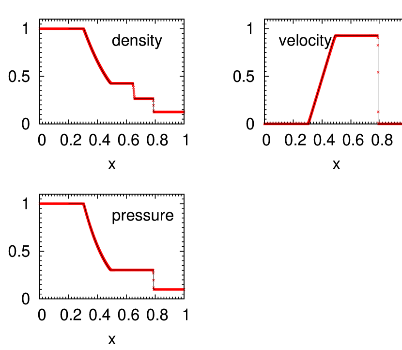
Figure 52.— Numerical results (red crosses) of the 1D-Riemann problem on the reference solutions (black lines) at $t=0.164$

.2. Riemann Problem in 2D

In order to test a multi-dimensional HD computation, a Riemann problem in 2D is carried out. A square numerical domain $(x,y)\in[0,1]\times[0,1]$ is divided into the four parts, and constant hydrodynamical values are set in each part. The initial condition is

$$\left(\begin{array}[]{c}\rho\\ p\\ v_{x}\\ v_{y}\end{array}\right) = \left(\begin{array}[]{c}1.0\\ 0.8\\ 0.0\\ 0.0\end{array}\right)\hskip 12.0pt\textrm{for}\hskip 12.0ptx<0.5\hskip 12.0pt\textrm{and}\hskip 12.0pty<0.5,$$ (22)

$$\left(\begin{array}[]{c}\rho\\ p\\ v_{x}\\ v_{y}\end{array}\right) = \left(\begin{array}[]{c}1.0\\ 1.0\\ 0.7276\\ 0.0\end{array}\right)\hskip 12.0pt\textrm{for}\hskip 12.0ptx<0.5\hskip 12.0pt\textrm{and}\hskip 12.0pty>0.5,$$ (31)

$$\left(\begin{array}[]{c}\rho\\ p\\ v_{x}\\ v_{y}\end{array}\right) = \left(\begin{array}[]{c}1.0\\ 1.0\\ 0.0\\ 0.7276\end{array}\right)\hskip 12.0pt\textrm{for}\hskip 12.0ptx>0.5\hskip 12.0pt\textrm{and}\hskip 12.0pty<0.5,$$ (40)

$$\left(\begin{array}[]{c}\rho\\ p\\ v_{x}\\ v_{y}\end{array}\right) = \left(\begin{array}[]{c}0.4\\ 0.5313\\ 0.0\\ 0.0\end{array}\right)\hskip 12.0pt\textrm{for}\hskip 12.0ptx>0.5\hskip 12.0pt\textrm{and}\hskip 12.0pty>0.5,$$ (49)

which is symmetric across a diagonal line $y=x$. An adiabatic index of $\gamma=1.4$ is used here. These setups are same with Case 12 of Liska (2003). The calculation is done with $400\times 400$ numerical cells. A numerical result is shown in Fig. 53, which is good agreement with that of Liska (2003).

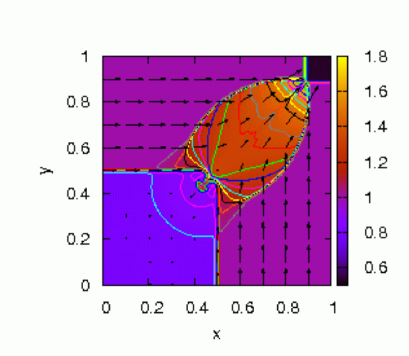
Figure 53.— Numerical result of the 2D-Riemann problem at $t=0.25$ (density color map with contours and velocity field vectors). The computation is done with $400\times 400$ cells.

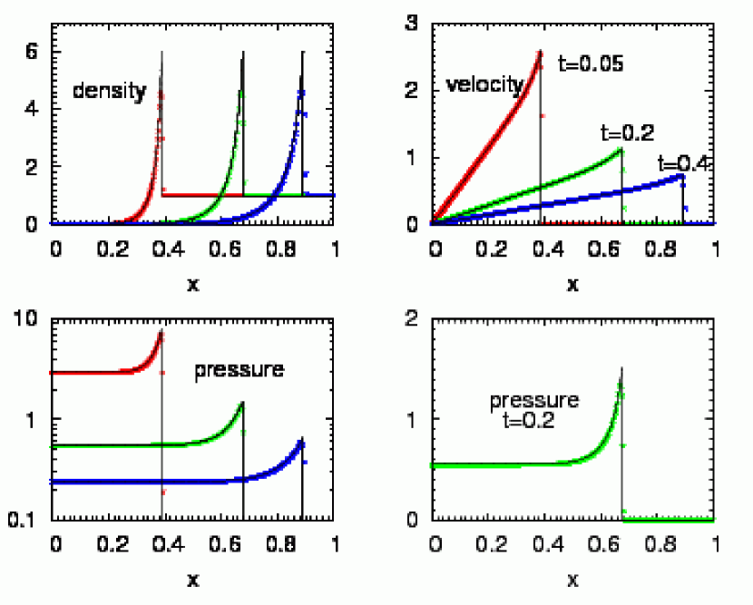
Figure 54.— Numerical results of a point source spherical explosion for density (left-top), velocity (right-top), and pressure (left-bottom) distribution. The right-bottom panel is shown to see, with linear scale, a sharpness of the numerical solution for pressure. In each figure, the red, green, and blue crosses represent solutions at $t=0.05$, $0.2$, and $0.4$, respectively.

.3. Point Source Spherical Explosion

Another HD test calculation we have done is a spherical point source explosion, the solution of that known as the Sedov’s solution. An 1D spherically symmetric computation is done with polar coordinate. We use non-uniform numerical cells with the spatial resolution of the $i$-th cell being $\Delta r_{i}=\Delta r_{\textrm{min}}\alpha^{i-1}$, where $\Delta r_{\textrm{min}}=10^{-4}$, $\alpha=1.0056$, and the maximum of $i$ is 720. This cell distribution is similar to that of the MHD core-collapse simulations presented in the present work, where the same cell distributions are set along the $\varpi$ and $z$ directions separately. Hence, we may be able to speculate here how much a propagating shock wave diffuses in our MHD core-collapse simulations. We put a static sphere of radius $r=1.0$ with the uniform density of $\rho_{0}=1.0$. A point source explosion is initiated by injecting the internal energy of $E_{0}=3.0$ at the central sphere of radius $r=0.01$. Numerical results are shown in Fig 54. It is found that a sharpness of density peak in the numerical solution is kept during propagation, despite that the spatial resolution is lower for a larger radius. This implies that, in our computations, a propagating shock wave is not damped crucially due to a numerical diffusion.

.4. Self-Similar Collapse

In order to check gravity is correctly dealt in Yamazakura, we tested a self-similar collapse, the solution of that known as Yahil’s solution (Yahil, 1983). Both an 1D spherically symmetirc calculation with polar coordinate and a 2D axially symmetric calculation with cylindrical coordinate are done. In describing Yahil’s solution, a radius, density, and velocity are written in dimensionless form:

$$R = \kappa^{-1/2}G^{(\gamma-1)/2}r(t_{0}-t)^{\gamma-2}$$

$$D(R) = \rho G(t_{0}-t)^{2}$$ (51)

$$V(R) = v\kappa^{-1/2}G^{(\gamma-1)/2}(t_{0}-t)^{\gamma-1},$$

where $G$, $\gamma$, $\kappa$, and $t_{0}$ are respectively the gravitational constant, adiabatic index, polytrope coefficient, and the time when the central density diverge. We put $\gamma=1.3$, $\kappa=1.2435\times 10^{15}/2^{4/3}$ cgs, and $t_{0}$ = 0.1 s. The collapse of a sphere with 4000 km radius is followed. In the cylindrical coordinate calculations, two different spatial resolutions are tested, where the resolutions of the inner-most cells are $\{\Delta\varpi_{\rm{min}},\Delta z_{\rm{min}}\}=2\times 10^{4}$ and $4\times 10^{4}$ cm. The number of numerical cells are $N_{\varpi}\times N_{z}=720\times 720$ in the both calculations. In the polar coordinate calculation, only one spatial resolution, $\Delta r_{\rm{min}}=4\times 10^{4}$ cm, with $N_{r}=720$ are taken.

The distributions of density and velocity when the central density reaches $2.3\times 10^{14}$ g cm^-3 are presented in Fig. 55, while errors at the inner most numerical cells are shown in Table 2. Note that, in our MHD core-collapse simulations, a bounce occurs when the central density reaches $\sim 2\times 10^{14}$ g cm^-3. Although the spherical collapse of the 15 $M_{\odot}$ progenitor used in the present work is not very well described by Yahil’s solution, the results obtained here may indicate how much error our collapse simulations involve. From the left panel of Fig. 55 one can see that, a deviation from the analytic solution is large near the center in each calculation. In the cylindrical coordinate calculation with $\{\Delta\varpi_{\rm{min}},\Delta z_{\rm{min}}\}=4\times 10^{4}$ cm, in which the grid construction is same with our standard MHD collapse simulations, the errors both in $D$ and $V$ are $\sim 10$ % (see the second row of Table 2). Although these errors seem too large to pursue a proper numerical simulation, as discussed in § 4.1.5, varying the spatial resolution in a MHD collapse simulation does not change results very much. This implies that the errors around the center are not fatal to the extent of the discussions developed in this paper.

As seen in Fig. 55 and in Table 2, the cylindrical coordinate calculations have larger errors than the polar coordinate calculation does, which may be due to the structure of numerical cells. However, we found that numerically evaluated electric currents behave better in cylindrical coordinate than in polar coordinate, and thus adopt the former in the present MHD simulations.

Table 2Errors in numerical solution at the inner-most cell.

Coordinate	$\{\Delta r_{\rm{min}},\Delta\varpi_{\rm{min}},\Delta z_{\rm{min}}\}$ [cm]	D-error [%]	V-error [%]
Cylindrical	$2\times 10^{4}$	7.28	22.0
Cylindrical	$4\times 10^{4}$	13.1	22.9
Polar	$4\times 10^{4}$	4.18	1.22

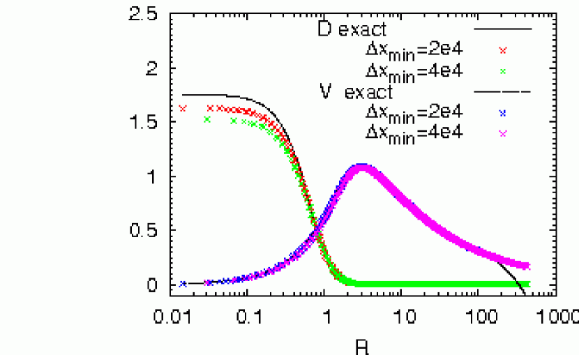
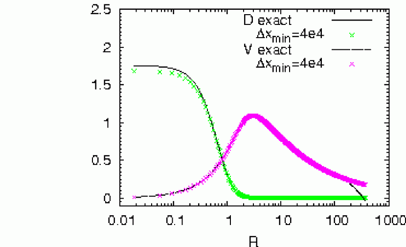
Figure 55.— Results for the calculations of the Yahil’s self-similar collapse with cylindrical coordinate (left) and polar coordinate (right). The solid lines and dotted lines are, respectively, for the analytic solution of D and V, while the colored crosses represent the numerical ones. For the cylindrical coordinate calculations, the numerical solutions along the pole ($\varpi$=0) are shown.

.5. MHD Riemann Problem

As a basic test for the ideal-MHD part of our code, we carried out a 1D-MHD Riemann problem that are known as Brio-Wu Problem (Brio & Wu, 1988). The initial condition is set as follows;

$$\left(\begin{array}[]{c}\rho\\ p\\ B_{x}/\sqrt{4\pi}\\ B_{y}/\sqrt{4\pi}\end{array}\right)=\left(\begin{array}[]{c}1.0\\ 1.0\\ 0.75\\ 1.0\end{array}\right)\hskip 12.0pt\textrm{for}\hskip 12.0ptx<0.5, \left(\begin{array}[]{c}\rho\\ p\\ B_{x}/\sqrt{4\pi}\\ B_{y}/\sqrt{4\pi}\end{array}\right)=\left(\begin{array}[]{c}0.125\\ 0.1\\ 0.75\\ -1.0\end{array}\right)\hskip 12.0pt\textrm{for}\hskip 12.0ptx>0.5$$ (68)

where the computational domain is $x\in[0,1]$. The initial velocities are set to be zero. The adiabatic index here is 2.0. The results of the calculation at $t=0.1$ done with 800 numerical cells are given in Fig. 56 together with those obtained by a famous numerical code ZEUS-2D (Stone & Norman, 1992). Although a little differences can be found, the two results well matches.

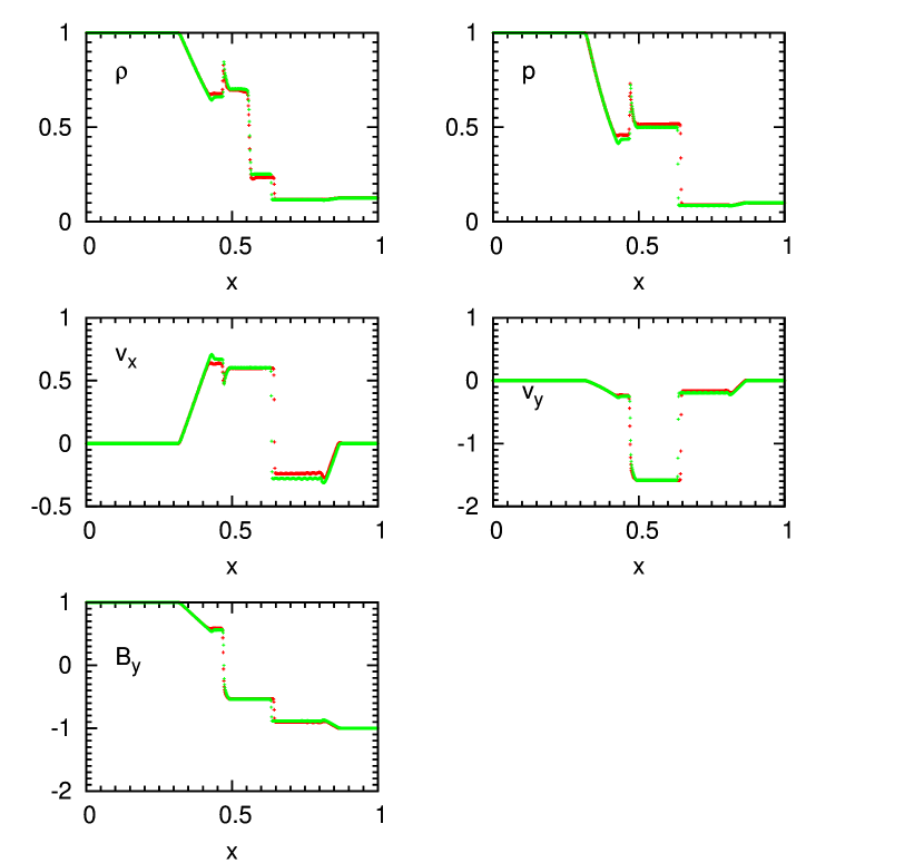
Figure 56.— Results of the MHD-Riemann problem at $t=0.1$. The red and Green crosses represent the solutions obtained by Yamazakura and ZEUS-2D, respectively. The both calculations are done with 800 numerical cells.

.6. Linear Wave Propagation

In § 2, we mentioned that the KT scheme adopted in our numerical code is third order in time and second order in space. Here, we will see whether Yamazakura solve the MHD equations fairly with these degree of accuracy, by carrying out a linear wave propagation problem in 1D Cartesian coordinate. A right-going slow magnetosonic wave is adopted as a linear wave.

According to Gardiner & Stone (2005), we put the initial state of the conserved variables as

$$\mbox{\boldmath$u$}_{in}=\mbox{\boldmath$u_{0}$}+\epsilon\mbox{\boldmath$R$}\cos(2\pi x),$$ (70)

where $u_{0}$ is the background state, $\epsilon=10^{-6}$ is the wave amplitude, and $R$ is the right eigenvector for the right-going slow magnetosonic wave in conserved variables given by

$$\mbox{\boldmath$R$}=\frac{1}{6\sqrt{5}}\left(\begin{array}[]{c}12\\ 6\\ 8\sqrt{2}\\ 4\\ 9\\ 0\\ -4\sqrt{2}\\ -2\end{array}\right).$$ (79)

The background state is set as $\rho_{0}=1$, $p_{0}=1$, $v_{0x}=v_{0y}=v_{0z}=0$, $B_{0x}=1$, $B_{0y}=\sqrt{2}$, and $B_{0z}=1/2$, with which the slow magnetosonic speed is $c_{s}=1/2$. The adiabatic index is set as $\gamma=5/3$. The computational domain is $x\in[0,1]$, and the periodic boundary condition is adopted at each boundary. Each calculation is run until $t=4$ when the wave has propagated the distance of two wave length.

In order to check the degree of accuracy in space, we first tested two calculation serieses with uniform cell construction, each of which contains four calculations with different grid numbers. In the first series, series A, we fix $\Delta t$ by controlling the Courant-Friedrichs-Lewy (CFL) number while varying $\Delta x$. The numbers of cells N and CFL numbers $\nu$ for the four calculations are $(N,\nu)=(8,0.49/64),(32,0.49/16),(128,0.49/4)$, and $(512,0.49)$. In the second series, series B, we fix the CFL number at $\nu=0.49$ and tested the same set of the cell numbers as before. Note that in series B, both $\Delta x$ and $\Delta t$ are halved by doubling the cell number. The distributions of $v_{x}$ at $t=4$ for series B are plotted in Fig. 57, which shows that the numerical solution well matches the analytic one for $N\geq 128$. The error from the analytic solution is evaluated by the L1 error norm,

$$|\delta\mbox{\boldmath$u$}|=\sqrt{\sum_{m}(\delta u^{m})^{2}},$$ (80)

where

$$\delta u^{m}=\frac{1}{N}\sum_{i}|u^{m}_{i}-(u^{m}_{in})_{i}|.$$ (81)

The left panel of Fig. 58 plots the variation of L1 error norm with respect to $N$ for series A and B. The red plots (series A) show that the scheme is approximately second order in space. We found that the results from series B (blue plots) are almost identical to those in series A, despite that $\Delta t$ is larger in series B for a fixed $N$, viz. a fixed $\Delta x$, except for $N=512$. This indicate that an error due to $\Delta t$ is dominated over by an error due to $\Delta x$ for $\nu<0.5$ (the CFL condition for the KT scheme), and brings difficulty in properly checking the degree of accuracy in time. Nonetheless, we can still state that the scheme is at least approximately second order in time, by the fact that the L1 error norms in series B, varying both $\Delta x$ and $\Delta t$ at a same rate, result in $\sim N^{-2}$ (see the blue plots in the left panel of Fig. 58).

Next, we evaluate the degrees of accuracy of our code for cases of non-uniform cell construction. A structure of numerical cells we set here is such that the $(2n-1)$-th cell has the size $L/N\times(1-\alpha)$ while the $2n$-th cell has the size $L/N\times(1+\alpha)$, where $L$ is the size of the whole numerical domain and $\alpha<1$ is the parameter to represent the degree of non-uniformity. We tested three cases $\alpha=10^{-2},10^{-1}$, and $5\times 10^{-1}$. In each case, four calculations fixing $\nu=0.49$ with $N=8,32,128$, and $512$ are done. The results are plotted in the right panel of Fig. 58. It is shown that the second order in space and at least second order in time are marginally kept even for 200 % size increase and 33 % size decrease from the neighboring cell ($\alpha=5\times 10^{-1}$). Note that a numerical cell size in our MHD-collapse simulations increases outwards by $0.56~{}\%$.

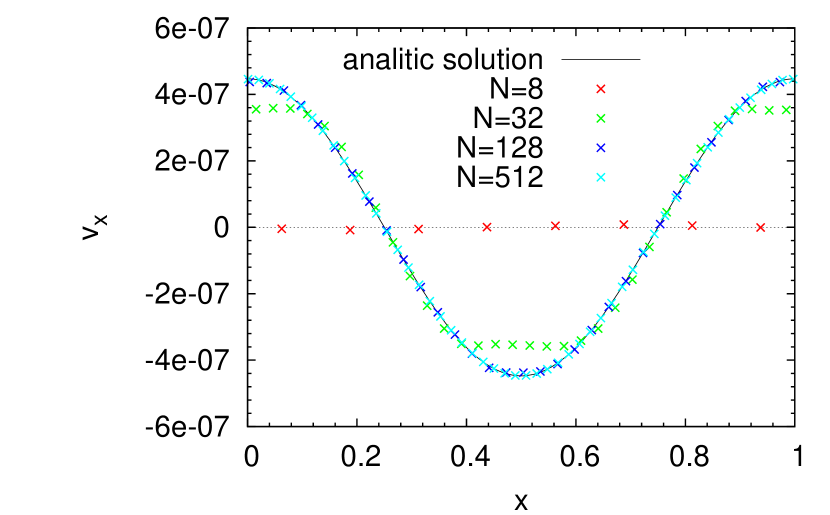
Figure 57.— Numerical results of the linear slow magnetosonic wave propagation for series A for the distribution of $v_{x}$ at $t=4$. The plots for the calculations with $N=128$ and 512 are thinned for the purpose of clear illustration.

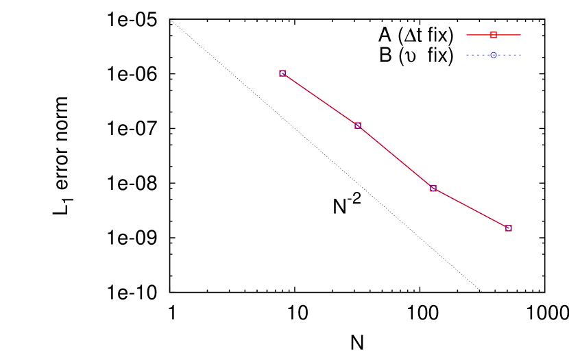
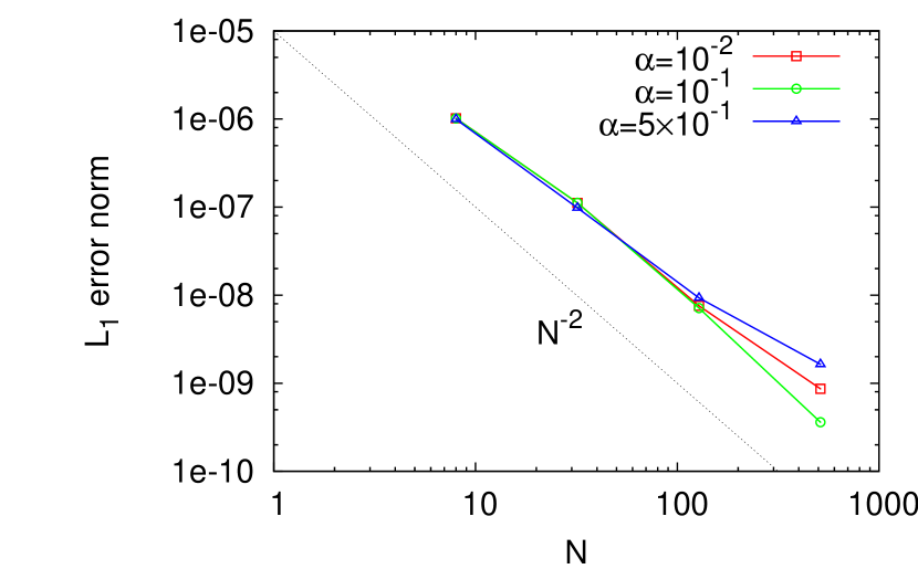
Figure 58.— Distributions of L1 error norm with respect to the number of numerical cells for the linear slow magnetosonic wave propagation problem with uniform cell spacing (left) and non-uniform cell spacing (right).

.7. Rotor Problem

In order to check that the multi-dimensional ideal MHD equations are well solved with our code, we perform two test calculations. One is a so-called rotor problem to be presented here, and the other is a point source explosion with magnetic field that will be shown in the next section.

The rotor problem is suggested by Balsara & Spicer (1999), which simulates the propagations of torsional Alfvén waves. The system initially consists of a rapidly rotating cylinder of dense fluid surrounded by lighter gas at rest, which is threaded by uniform a magnetic field parallel to the $x$-axis. With the computational domain of $(x,y)\in[-0.5,0.5]\times[-0.5,0.5]$, the initial condition is

$$\rho = 1+9f(r),$$

$$p = 1,$$

$$v_{x} = -2f(r)y/r,\hskip 12.0ptv_{y}=-2f(r)x/r,\hskip 12.0ptv_{z}=0,$$

$$B_{x} = 5,\hskip 12.0ptB_{y}=B_{z}=0,$$ (82)

where

$$f(r) = \begin{cases}1&\textrm{if}\hskip 12.0ptr<0.1,\\ \frac{200}{3}(0.115-r)&\textrm{if}\hskip 12.0pt0.1<r<0.115,\\ 0&\textrm{if}\hskip 12.0ptr>0.115,\end{cases}$$

$$r = (x^{2}+y^{2})^{1/2}.$$

The adiabatic index is $\gamma=1.4$. The calculation is done with $400\times 400$ numerical cells. Results of the calculation are displayed in Fig. 59, which show good agreement with those found in Ziegler (2004).

Figure 59.— Numerical results of the rotor problem. Left and Right panels respectively show pressure and Mach number contours at $t=0.15$

Figure 60.— Magnetic pressure contours at $t=2.5\times 10^{-3}$ in the calculation of a point source explosion with magnetic field.

.8. Point Source 3D-Explosion with Magnetic Field

A calculation presented here differs from the spherical explosion test described above in that fluid is magnetized. The initial condition is given by

$$\rho = 1,$$

$$p = \begin{cases}10^{4}&\textrm{if}\hskip 12.0ptx^{2}+y^{2}+z^{2}<r^{2},\\ 1&\textrm{otherwise.}\end{cases}$$

$$v_{x} = v_{y}=v_{z}=0,$$

$$B_{z}/\sqrt{4\pi} = 100,\hskip 12.0ptB_{x}=B_{y}=0.$$ (83)

The adiabatic index is chosen as $\gamma=5/3$. We do a calculation in cylindrical coordinate with the numerical domain of $(\varpi,z)\in[0,0.5]\times[0,0.5]$, taking the symmetric axis in the magnetic field direction. The number of numerical cells is $N_{\varpi}\times N_{z}=96\times 96$. A result of the calculation is given in Fig. 60. This also shows good agreement with that of Ziegler (2004) done with Cartesian coordinate.

.9. Magnetic Field Diffusion

In order to see that Yamazakura properly handles the resistive terms in the induction equation, we test a magnetic field diffusion problem in 1D. Here, we solve not the full set of the MHD equations but the magnetic diffusion equation with a constant resistivity,

$$\frac{\partial B}{\partial t} = \eta\frac{\partial^{2}B}{\partial x^{2}},$$ (84)

by freezing fluid in the induction equation. Setting the initial condition with an anti-parallel magnetic field, $B=-B_{0}$ for $x<0$ and $B=B_{0}$ for $x>0$, the exact solution at time $t$ is written as

$$B(x,t) = -\frac{2B_{0}}{\sqrt{\pi}}\int^{x/\sqrt{4\eta t}}_{0}e^{-u^{2}}du\hskip 12.0pt\textrm{for}\hskip 12.0ptx<0,$$

$$B(x,t) = \frac{2B_{0}}{\sqrt{\pi}}\int^{x/\sqrt{4\eta t}}_{0}e^{-u^{2}}du\hskip 12.0pt\textrm{for}\hskip 12.0ptx>0.$$ (85)

We set $B_{0}=100$ and $\eta=10$. The calculation is done with 800 numerical cells for $x\in[-5,5]$. The Results are displayed in Fig. 61, in which one can find good agreement between the numerical and exact solutions.

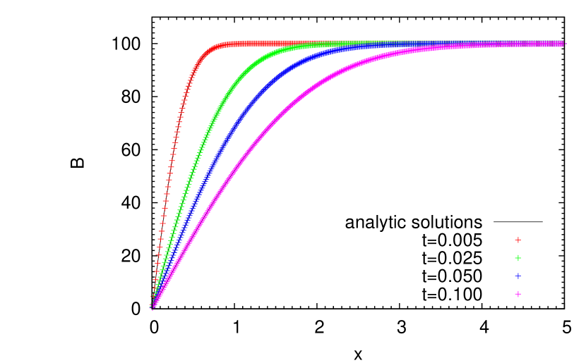
Figure 61.— Results of the magnetic field diffusion calculation. The numerical solutions are shown by the crosses while the analytic solutions are by the solid lines.

.10. Spontaneous Fast Reconnection

We finally check that Yamazakura properly deals with the multi-dimensional resistive-MHD equations, by the simulation of a spontaneous fast reconnection firstly done by Ugai (1999). The initial current system is constructed as follows:

$$B_{x}(y)/\sqrt{4\pi} = \begin{cases}\sin(\pi y/2)&\textrm{for}\hskip 12.0pty<1,\\ 1&\textrm{for}\hskip 12.0pt1<y<3.6,\\ \cos[(y-3.6)\pi/1.2]&\textrm{for}\hskip 12.0pt3.6<y<4.2,\\ 0&\textrm{for}\hskip 12.0pt4.2<y,\\ -B_{x}(-y)/\sqrt{4\pi}&\textrm{for}\hskip 12.0pty<0,\\ \end{cases}$$

$$p = (1+\beta_{0}-B_{x}^{2}/4\pi)/2,$$

$$\rho = 2p/(1+\beta_{0}),$$ (86)

where $\beta_{0}=0.15$. A velocity and the $x,y$-component of magnetic field are initially zero. The adiabatic index is taken as $\gamma=5/3$. A reconnection of magnetic field-lines is initiated by an anomalous resistivity;

$$\eta(\mbox{\boldmath$r$},t) = \begin{cases}k_{R}[V_{d}(\mbox{\boldmath$r$},t)-V_{c}]&\textrm{for}\hskip 12.0ptV_{d}>V_{c},\\ 0&\textrm{for}\hskip 12.0ptV_{d}<V_{c},\\ \end{cases}$$ (87)

where

$$V_{d}(\mbox{\boldmath$r$},t) = \left|\mbox{\boldmath$J$}(\mbox{\boldmath$r$},t)/\rho(\mbox{\boldmath$r$},t)\right|,$$

$$V_{c} = V_{c,0}\left[\frac{2p}{\rho(1+\beta_{0})}\right]^{\alpha}.$$ (89)

The parameters are taken as $k_{R}=0.03$, $V_{c,0}=4$, and $\alpha=0.5$. For details of the resistivity model, see Ugai (1999). The anomalous resistivity model (87) is assumed for $t>4$. During $0<t<4$, a localized resistivity bellow is imposed to disturb the initial 1D-configuration:

$$\eta(\mbox{\boldmath$r$}) = \eta_{d}\exp[-(x/1.1)^{2}-(y/1.1)^{2}],$$ (90)

where $\eta_{d}=0.02$. The computation is done with $800\times 800$ numerical cells covering the domain of $(x,y)\in[-20,20]\times[-6,6]$.

Some important results of the computation are shown in Fig. 62 and 63. The global magnetic-field distributions are displayed in Fig. 62 for t=18 and 30. We found that they are similar to those obtained by Ugai (1999), and also those of Feng et al. (2006). The left panel of Fig. 63 represents profiles of $v_{x}$ and $B_{y}$ along the x-axis at $t=24$ and $t=30$, while the right panel shows the evolution of the resistivity $\eta$ and electric field $E$ at the origin, $v_{y}$ at $(x,y)=(0,0.9)$, and a magnetic flux $\Phi$ evaluated by

$$\Phi=\int_{y\geq 0}B_{x}(x=0,y)dy.$$

For these results, we also find a rough agreement with the above two works, although there are some insignificant differences.

With all these results presented in the appendix, we expect that the present MHD collapse simulations done by Yamazakura offer proper results.

Figure 62.— Magnetic field distributions at t=18 and 30 for the calculation of spontaneous fast reconnection.

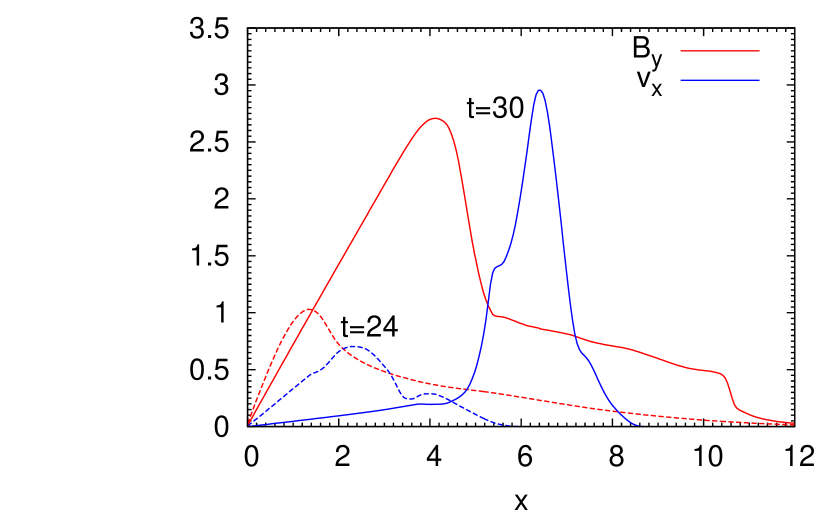
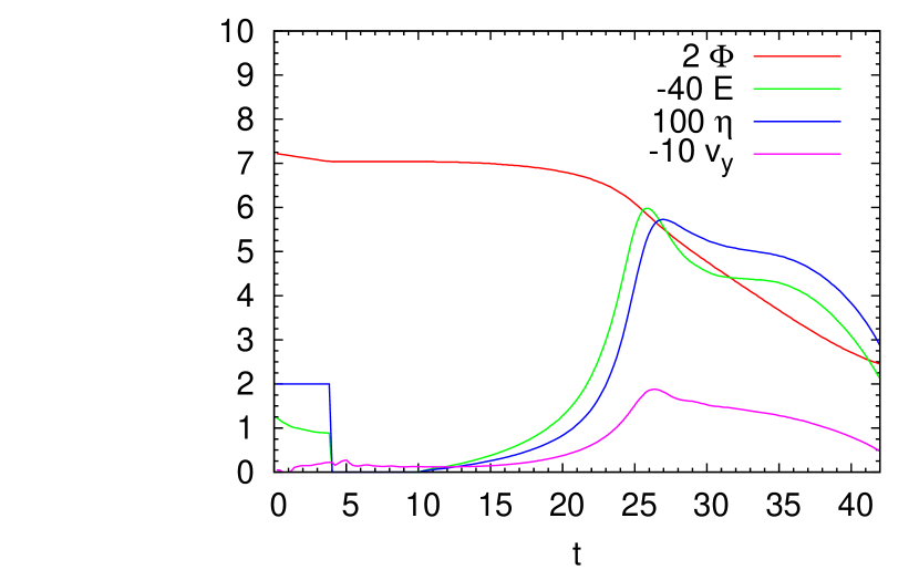
Figure 63.— Results for the calculation of spontaneous fast reconnection. Left: Profiles of $v_{x}$ and $B_{y}$ along the x-axis at $t=24$ and $t=30$. Right: Temporal variations of the magnetic flux $\Phi$, the resistivity $\eta$ and electric field $E$ at the origin, and $v_{y}$ at $(x,y)=(0,0.9)$.

References

- Akiyama et al. (2003) Akiyama, S., Wheeler, J. C., Meier, D. L., & Lichtenstadt, I. 2003, ApJ, 584, 954
- Aurière et al. (2010) Aurière, M., Donati, J.-F., Konstantinova-Antova, R., et al. 2010, A&A, 516, L2
- Balbus (1995) Balbus, S. A. 1995, ApJ, 453, 380
- Balbus & Hawley (1991) Balbus, S. A., & Hawley, J. F. 1991, ApJ, 376, 214
- Balsara & Spicer (1999) Balsara, D. S., & Spicer, D. S. 1999, J. Chem. Phys., 149, 270
- Braithwaite (2009) Braithwaite, J. 2009, MNRAS, 397, 763
- Brandenburg & Subramanian (2005) Brandenburg, A., & Subramanian, K. 2005, Phys. Rep., 417, 1
- Brio & Wu (1988) Brio, M., & Wu, C. C. 1988, Journal of Computational Physics, 75, 400
- Burrows et al. (2007) Burrows, A., Dessart, L., Livne, E., Ott, C. D., & Murphy, J. 2007, ApJ, 664, 416
- Diehl et al. (2006) Diehl, R., Halloin, H., Kretschmer, K., et al. 2006, Nature, 439, 45
- Donati et al. (2006) Donati, J.-F., Howarth, I. D., Bouret, J.-C., et al. 2006, MNRAS, 365, L6
- Endeve et al. (2012) Endeve, E., Cardall, C. Y., Budiardja, R. D., et al. 2012, ApJ, 751, 26
- Evans & Hawley (1988) Evans, C. R., & Hawley, J. F. 1988, ApJ, 332, 659
- Feng et al. (2006) Feng, X., Hu, Y., & Wei, F. 2006, Sol. Phys., 235, 235
- Ferrario & Wickramasinghe (2006) Ferrario, L. & Wickramasinghe, D. T. 2006, Mon. Not. Astron. Soc., 367, 1323
- Foglizzo et al. (2006) Foglizzo, T., Scheck, L., & Janka, H.-T. 2006, ApJ, 652, 1436
- Gardiner & Stone (2005) Gardiner, T. A., & Stone, J. M. 2005, Journal of Computational Physics, 205, 509
- Guilet et al. (2011) Guilet, J., Foglizzo, T., & Fromang, S. 2011, ApJ, 729, 71
- Gustafsson (1983) Gustafsson, I. 1983, “Modified incomplete Cholesky (MIC) methods”, in: D.J. Evans, ed., Preconditioning Methods; Theory and Applications (Gordon and Breach, New York), 265-293.
- Heger et al. (2005) Heger, A., Woosley, S. E., & Spruit, H. C. 2005, ApJ, 626, 350
- Herant et al. (1994) Herant, M., Benz, W., Hix, W. R., Fryer, C. L., & Colgate, S. A. 1994, ApJ, 435, 339
- Iwakami et al. (2009) Iwakami, W., Kotake, K., Ohnishi, N., Yamada, S., & Sawada, K. 2009, ApJ, 700, 232
- Kotake et al. (2004) Kotake, K., Sawai, H., Yamada, S., & Sato, K. 2004, ApJ, 608, 391
- Kurganov & Tadmor (2000) Kurganov, A., & E. Tadmor 2000, Journal of Computational Physics, 160, 241
- Kuroda & Umeda (2010) Kuroda, T., & Umeda, H. 2010, ApJS, 191, 439
- LeBlanc & Wilson (1970) LeBlanc, J. M., & Wilson, J. R. 1970, ApJ, 161, 541
- Leahy & Ouyed (2007) Leahy, D., & Ouyed, R. 2007, arXiv:0710.2114
- Liebendörfer (2005) Liebendörfer, M. 2005, ApJ, 633, 1042
- Liska (2003) Liska, R., & Wendroff, B. 2003, SIAM J. Sci. Comput. 25, 995
- Marek et al. (2009) Marek, A., Janka, H.-T., & Müller, E. 2009, A&A, 496, 475
- Masada et al. (2006) Masada, Y., Sano, T., & Takabe, H. 2006, ApJ, 641, 447
- Moiseenko et al. (2006) Moiseenko, S. G., Bisnovatyi-Kogan, G. S., & Ardeljan, N. V. 2006, MNRAS, 310, 501
- Murphy & Burrows (2008) Murphy, J. W., & Burrows, A. 2008, ApJ, 688, 1159
- Nordhaus et al. (2010) Nordhaus, J., Burrows, A., Almgren, A., & Bell, J. 2010, ApJ, 720, 694
- Obergaulinger et al. (2006) Obergaulinger, M., Aloy, M. A., & Müller, E. 2006, A&A, 450, 1107
- Obergaulinger et al. (2009) Obergaulinger, M., Cerdá-Durán, P., Müller, E., & Aloy, M. A. 2009, A&A, 498, 241
- Obergaulinger & Janka (2011) Obergaulinger, M., & Janka, H.-T. 2011, arXiv:1101.1198
- Papaliolios et al. (1989) Papaliolios, C., Krasovska, M., Koechlin, L., Nisenson, P., & Standley, C. 1989, Nature, 338, 565
- Sawai et al. (2005) Sawai, H., Kotake, K. & Yamada, S. 2005, ApJ, 631, 446
- Sawai et al. (2008) Sawai, H., Kotake, K. & Yamada, S. 2008, ApJ, 672, 465
- Shen et al. (1998a) Shen, H., Toki, H., Oyamatsu, K., & Sumiyoshi, K. 1998a, Nuclear Physics A, 637, 435
- Shen et al. (1998b) Shen, H., Toki, H., Oyamatsu, K., & Sumiyoshi, K. 1998b, Progress of Theoretical Physics, 100, 1013
- Shibata et al. (2006) Shibata, M., Liu, Y. T., Shapiro, S. L., & Stephens, B. C. 2006, Phys. Rev. D, 74, 104026
- Spitzer (1956) Spitzer, L. 1956, Physics of Fully Ionized Gases, New York: Interscience Publishers
- Spruit (2002) Spruit, H. C. 2002, A&A, 381, 923
- Stone & Norman (1992) Stone, J. M., & Norman M. L. 1992, ApJS, 80, 791
- Sumiyoshi et al. (2007) Sumiyoshi, K., Yamada, S., & Suzuki, H. 2007, ApJ, 667, 382
- Sumiyoshi et al. (2005) Sumiyoshi, K., Yamada, S., Suzuki, H., Shen, H., Chiba, S., & Toki, H. 2005, ApJ, 629, 922
- Symbalisty (1984) Symbalisty, E. M. D. 1984, ApJ, 285, 729
- Takiwaki et al. (2004) Takiwaki, T., Kotake, K., Nagataki, S., & Sato, K. 2004, ApJ, 616, 1086
- Takiwaki et al. (2009) Takiwaki, T., Kotake, K., & Sato, K. 2009, ApJ, 691, 1360
- Thompson & Duncan (2003) Thompson, C., & Duncan, R. C. 1993, ApJ, 408, 194
- Thompson et al. (2005) Thompson, T. A., Quataert, E., & Burrows, A. 2005, ApJ, 620, 861
- Ugai (1999) Ugai, M. 1999, Phys. Plasmas, 6, 1522
- Wade et al. (2012) Wade, G. A., Grunhut, J., Gräfener, G., et al. 2012, MNRAS, 419, 2459
- Wang et al. (2001) Wang, L., Howell, D. A., Höflich, P., & Wheeler, J. C. 2001, ApJ, 550, 1030
- Woosley & Heger (2006) Woosley, S. E., & Heger, A. 2006, ApJ, 637, 914
- Yahil (1983) Yahil, A. 1983, ApJ, 265, 1047
- Yamada & Sawai (2004) Yamada, S., & Sawai, H. 2004, ApJ, 608, 907
- Yoshizawa (1990) Yoshizawa, A. 1990, Phys. Fluids B, 2, 1589
- Ziegler (2004) Ziegler, U. 2004, Journal of Computational Physics, 196, 393