SCALABLE SPECTRAL ALGORITHMS FOR COMMUNITY DETECTION IN DIRECTED NETWORKS

Abstract

Community detection has been one of the central problems in network studies and directed network is particularly challenging due to asymmetry among its links. In this paper, we found that incorporating the direction of links reveals new perspectives on communities regarding to two different roles, source and terminal, that a node plays in each community. Intriguingly, such communities appear to be connected with unique spectral property of the graph Laplacian of the adjacency matrix and we exploit this connection by using regularized SVD methods. We propose harvesting algorithms, coupled with regularized SVDs, that are linearly scalable for efficient identification of communities in huge directed networks. The proposed algorithm shows great performance and scalability on benchmark networks in simulations and successfully recovers communities in real network applications.

arXiv:1211.6807

and

t1Partially supported by NSF grant (DMS-1007060 and DMS-130845)

1 INTRODUCTION

Many real world problems can be effectively modeled as pairwise relationship in networks where nodes represent entities of interest and links mimic the interactions or relationships between them. The study of networks, recently referred to as network science, can provide insight into their structures and properties. One particularly interesting problem in network studies is searching for important sub-networks which are called communities, modules or groups. A community in a network is typically characterized by a group of nodes that have more links connected within the community than connected to other nodes (Fortunato, 2010).

In many practical applications, the networks in study are directed in nature, such as the World Wide Web, tweeter’s follower-followee network, and citation networks. Compared with in-depth studies of community structures in undirected networks (Danon et al., 2005; Fortunato, 2010; Coscia, Giannotti and Pedreschi, 2011), community detection in directed networks has not been as fruitful. We found that one particular reason is a restrictive assumption on the community structure in a directed network. Many of previous studies assumed a member of a community has balanced out-links and in-links connected to other members. This symmetric assumption can be seriously violated in cases where a member may only play one main role, source or terminal, in the community.

We give an example of such violation, Cora citation network, which presents bibliographic citations among papers in computer science. Citation networks have temporal restriction and it make them difficult to form symmetric communities. The left panal of Figure 1 illustrates communities detected by a popular Infomap algorithm (Rosvall, Axelsson and Bergstrom, 2009) which assumes symmetric communities. We see that it only detects minuscule symmetric communities. On the other hand, the right panel of Figure 1 reveals a completely different community structure that turned out to show high correspondance to the categories of the papers. This result is obtained by relaxing the symmetric assumption and allowing two different roles for a node in a community. We defer our discussion on details of this example to Section 5.1.

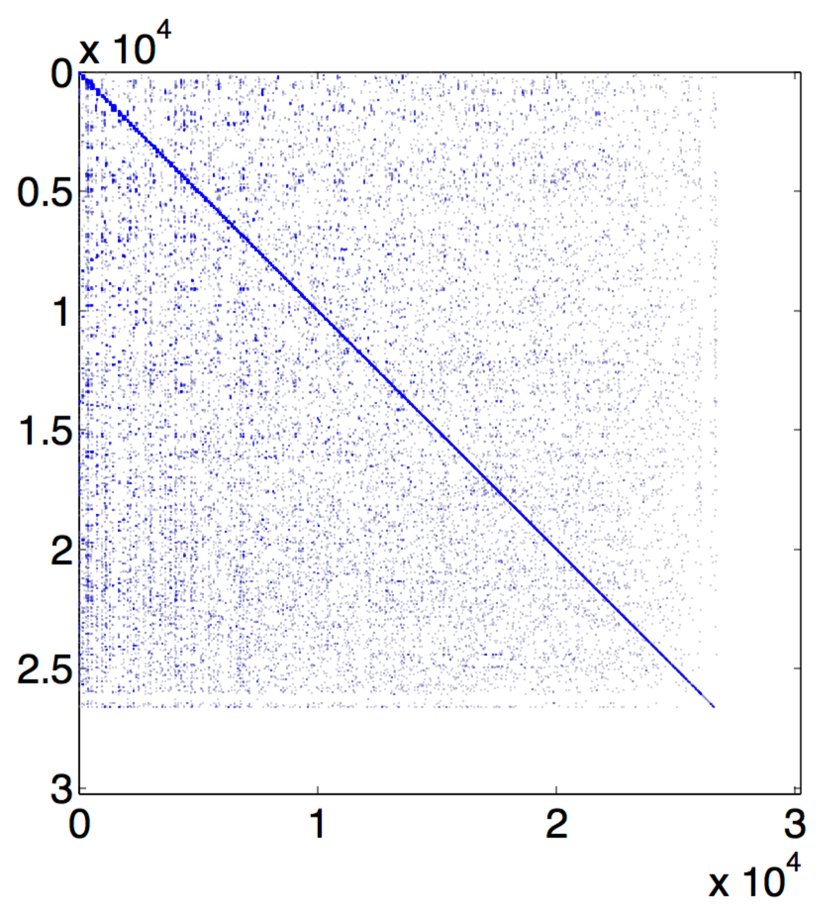
(a) Infomap

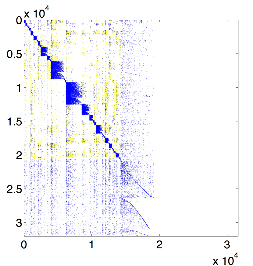
(b) $L_{0}$-harvesting

Figure 1: Comparison of symmetric communities detected by Infomap and asymmetric communities detected by the proposed algorithm in Cora citation network. See Section 5.1.1 for more details.

Asymmetric communities are common in directed networks where the direction implicitly express an asymmetric relationship among its nodes. For example, social networks show celebrity-fan community structure and celebrities hardly follow many fans. Satuluri and Parthasarathy (2011) and Guimerà, Sales-Pardo and Amaral (2007) also pointed out such asymmetric communities in the context of World-Wide-Web, a Wikipedia network and investment networks.

In this paper, we show that a community structure driven by two separate roles that a node plays in a directed network can be formulated as a paired sets of nodes. We call such community, Directional Community, which is defined by a paired sets of nodes, a source node set and a terminal node set. We investigate notions of connectivity and quality measures for a directional community. In those aspects, we propose algorithms that is capable of detecting good directional communities.

Another aspect of a community detection algorithm we consider here is scalability. Huge networks raise two concerns, computational complexity and computer memory requirements. We exploit regularized Singular Value Decomposition (SVD) and search local communities in time proportional to the number of edges.

The remainder of this paper is organized as follows: Section 2 introduces a new concept of community for directed networks. Section 3 presents the regularized SVD algorithms developed for detecting the communities. A simulation study is presented in Section 4. Section 5 shows the results of the proposed algorithms in two real-world networks. We finish with conclusions in Section 6. Due to limitations of space, proofs of all theoretical results are included in Appendix.

2 COMMUNITY IN A DIRECTED NETWORK

The nodes and links in a directed network are often presented by a graph ${\cal G}=({\cal V},{\cal E})$, with ${\cal V}\equiv\{v_{1},\ldots,v_{n}\}$ and ${\cal E}\equiv\{e_{1}\ldots,e_{m}\}$ denoting the vertex set and edge set respectively. For an existing edge $e$ in the network, its source node and terminal node are denoted as $v^{s}(e)$ and $v^{t}(e)$ respectively. Let $W$ be the $|{\cal V}|\times|{\cal V}|$ adjacency matrix in which $W(i,j)=1$ indicates the existence of an edge originated from $v_{i}$ and pointed to $v_{j}$ and $W(i,j)=0$ otherwise.

In the literature of community detection in directed networks, several authors have attempted to directly incorporate the directionality of edges into their algorithms (Capocci et al., 2005; Newman and Leicht, 2007; Andersen and Lang, 2006; Arenas et al., 2007; Rosvall, Axelsson and Bergstrom, 2009). In particular, existing works pointed out the importance of recognizing the dual roles, source and terminal of edges. (Zhou, Schölkopf and Hofmann, 2005; Guimerà, Sales-Pardo and Amaral, 2007; Benzi, Estrada and Klymko, 2012).

We consider a community structure that treats the dual roles separately. A Directional Community $C(S,T)$ is defined by two different sets of nodes, a source node set $S\subset{\cal V},S\neq\emptyset$, and a terminal node set $T\subset{\cal V},T\neq\emptyset$. Community structure is characterized by majority of edges placed within the community (starting from the nodes in $S$ and ending at the nodes in $T$). In what follows, we first define a new type of connectivity between nodes in a directed network. This newly defined connectivity leads to the concept of Directional Components, which serve as communities in the ideal situation in analogous to connected components in an undirected network. Furthermore, we consider a graph cut criterion that measures the quality of a directional community.

2.1 Directional Components

We start with exploring connectivities of nodes in a directed network. Two types of connectivity have been studied in directed networks. Weak connectivity defines two nodes $s$ and $t$ ($s,t\in\cal{V}$) as weakly connected if they can reach each other through a path, regardless of the direction of edges in the path. Meanwhile, Strong connectivity follows the direction of edges in a path and calls nodes $s$ and $t$ strongly connected if the path $(e_{1},e_{2},\ldots,e_{l})$ also satisfies $v^{s}(e_{1})=s,v^{t}(e_{l})=t,v^{t}(e_{k})=v^{s}(e_{k+1}),k=1,\dots,l-1$. In this paper, we propose a new type of connectivity,

Definition 2.1.

Two nodes $s$ and $t$ ($s,t\in\cal{V})$ are D-connected, denoted by $s\leadsto t$, if there exists a path of edges $(e_{1},\dots,e_{2m-1})$, $m\in\mathbb{R}^{+}$, satisfying $v^{s}(e_{1})=s,v^{t}(e_{2m-1})=t$ and

$$\begin{cases}v^{t}(e_{2k-1})=v^{t}(e_{2k})&\mbox{(common terminal nodes)}\\ v^{s}(e_{2k})=v^{s}(e_{2k+1})&\mbox{(common source nodes)}\end{cases}$$

for $k=1,2,\ldots,\max\{m-1,1\}$.

D-connectivity follows the edges in alternating directions, first forward and then backward. We call this sequence of edges a D-connected path. Figure 2 provides an illustration of D-connectivity. For example, we observe that $A\leadsto D$ through a sequence of edges $(e_{2},e_{3},e_{4})$ and $E\leadsto A$ through a sequence of edges $(e_{5},e_{4},e_{1})$.

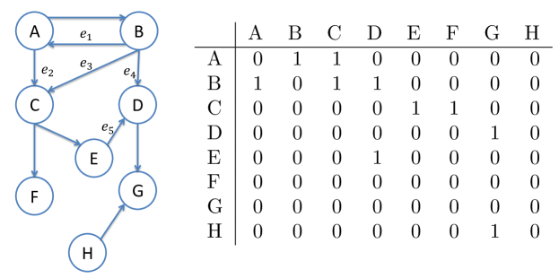
Figure 2: An example directed network and its adjacency matrix.

The definition of D-connectivity is a restricted version of a concept called alternating connectivity that was introduced by Kleinberg (1999) in the context of analyzing the centrality of web-pages of World Wide Web using the HITS algorithm. The difference is that the alternating connectivity allows two nodes be any pair on an alternating path regardless of their roles. Kleinberg also pointed out the difficulty of developing the alternating connectivity to a concept that characterizes a group of tightly connected nodes (a community), because transitive relation does not hold in alternating connectivity. However, D-connectivity bypasses this problem by recognizing the two different roles, source and terminal. Next we define a community structure, Directional Component, based on the D-connectivity.

Definition 2.2.

A Directional Component $(DC)$ consists of a source node set $S$ and a terminal node set $T$ $(S,T\subset\cal{V})$ and they are the maximal subsets of nodes such that any pair of nodes $(s,t),s\in S,t\in T$, are D-connected $(s\leadsto t)$. We call $S$ and $T$ the source part and terminal part of the directional component and denote $DC\equiv(S,T)$.

Directional components have desired properties as directional communities. First, there is no edges between the source part of one component and the terminal part of other components. Second, in a directed network that contains multiple directional components $DC_{1},DC_{2},\ldots,DC_{K}$, any node can belong to only one of the source parts. In other words, the source parts $S_{1},\ldots,S_{K}$ are disjoint and the same holds for $T_{1},\ldots,T_{K}$. Third, each edge belongs to one of directional components thus they give a partition of edges.

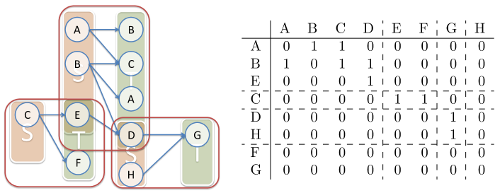
Figure 3: The decomposition of the network in Figure 2 and rearranged adjacency matrix.

This two-way partition of nodes respects the asymmetric property of a directed network. Figure 3 illustrates the decomposition of the directed network shown in Figure 2. Three directional components are found and the source and terminal parts of each directional component are displayed in boxes. A node may have different memberships as source or terminal. After reorganizing the nodes by directional components, there is no edges between the source part and the terminal part of different directional components, as shown in the right panel of Figure 3. This two-way partition of nodes results in a re-ordered adjacency matrix which exhibits block-wise structure.

A directional component may include the source part and the terminal part that share few common nodes. This asymmetricity is possible because the nodes in a D-connectivity path need to play only a single role, source or terminal. On the other hand, strong connectivity requires the nodes in a path, except the first and the last node, to be source and terminal at the same time. Therefore, it is not surprising that many existing works based on strong connectivity identify symmetric communities, for example Andersen, Chung and Lang (2007); Rosvall, Axelsson and Bergstrom (2009).

Finding directional components can be achieved through a simple searching algorithm of computational complexity $O(|\cal{V}|+|\cal{E}|)$. A directional component is identified by iteratively adding nodes into the source part and the terminal part (see Algorithm 3 in Appendix A). We use this algorithm to decompose a directed network into directional components prior to searching communities.

One drawback of searching for directional components is that real networks usually have only one large directional component and negligible small ones. This phenomenon is due to the fact that it is unrealistic to expect absolutely no links between those communities. In order to find more realistic communities, we first consider a quality measure of directional community under the presence of a small number of external edges.

2.2 Directional Conductance

We consider a graph cut criterion for directional communities and define directional cut between two directional communities $C_{k}(S_{k},T_{k}),C_{l}(S_{l},T_{l})$ as

$$\mbox{d-Cut}(C_{k}(S_{k},T_{k}),C_{l}(S_{l},T_{l}))=\sum_{v_{i}\in S_{k}}\sum_{v_{j}\in T_{l}}W_{ij}+\sum_{v_{i}\in S_{l}}\sum_{v_{j}\in T_{k}}W_{ij},$$ (2.1)

where $W$ is the adjacency matrix. Notice that two directional components have zero d-Cut.

We want to emphasize the difference of d-Cut from a graph cut studied in Meila and Pentney (2007). The graph cut criteria counts all links between two communities while d-Cut only counts the links starting from the source nodes of one community to the terminal nodes of the other and vice versa. Directional cut is equivalent to the graph cut criterion if $S_{k}=T_{k},S_{l}=T_{l}$.

Based on d-Cut, we propose a measure of the quality of a directional community, Directional Conductance,

$$\phi(C(S,T))=\frac{\mbox{d-Cut}(C(S,T),C(\bar{S},\bar{T}))}{\min\{\text{Vol}(S)+\text{Vol}(T),\text{Vol}(\bar{S})+\text{Vol}(\bar{T})\}},\\$$ (2.2)

where $\bar{S},\bar{T}$ denotes the complement set of $S$ and the complement set of $T$, respectively. $\mbox{Vol}(S)$ is defined as $\sum_{v_{i}\in S}d_{r,i}$, the sum of out-degrees of nodes in $S$ and $\mbox{Vol}(T)$ is $\sum_{v_{j}\in T}d_{c,j}$, the sum of in-degrees of nodes in $T$. The value of $\phi$ has a range from zero to one and a lower value indicates relatively fewer external edges. Note that the value of $\phi$ for a directional component is zero. There are alternative normalizations that can be defined using d-Cut, however, in this paper we concentrate on (2.2).

So far, we have explored the asymmetric roles of nodes in a directional component. The proposed D-connectivity preserves the roles along the alternating paths and directional components divide a directed network into groups according to the D-connectivity. The distinction between the source part and the terminal part of a directional community leads to the directional conductance. In the following sections, we develop scalable algorithms that identify directional communities under the consideration of the connectivity and the conductance.

3 REGULARIZED SVD ALGORITHMS FOR COMMUNITY EXTRACTION

Rohe and Yu (2012) proposed a DI-SIM algorithm that uses the low-rank approximation via SVD for bi-clustering (co-clustering) of nodes in a directed network. They investigated the spectrum of graph Laplacian of the adjacency matrix $W$. The graph Laplacian $Q$ is defined as

$$Q=D_{r}^{-\frac{1}{2}}WD_{c}^{-\frac{1}{2}},$$ (3.1)

where $D_{r}$ is the diagonal matrix of out-degrees $\{d_{r,i}\}_{i=1,\ldots,n}$, and $D_{c}$ is the diagonal matrix of in-degrees $\{d_{c,j}\}_{j=1,\ldots,n}$ . As a remark, the graph Laplacian $Q$ here is different from the graph Laplacian considered in Chung (2005); Boley, Ranjan and Zhang (2011), which is based on the strong connectivity of nodes. Assuming a known number of communities, the DI-SIM algorithm clusters nodes in two different ways by running the k-means algorithm on the leading left singular vectors and right singular vectors separately. They showed that the DI-SIM algorithm may recover stochastically equivalent sender-nodes and receiver-nodes under Stochastic Co-Block model, which is a relaxed version of Stochastic Block model of Holland, Laskey and Leinhardt (1983).

3.1 Regularized SVD with $L_{0}$ Penalty

In spite of DI-SIM algorithm’s solid theoretical basis, there are several limitations for our purpose on discovering directional communities in a huge directed network. First, it clusters nodes in two different clusters, but does not provide paired source nodes and terminal nodes. Second, it requires a pre-specified number of communities, which is unknown in most of applications. Third, the spectral clustering is not scalable and not easy to be parallelized. Huge networks frequently have many small communities (Leskovec et al., 2008) and it is challenging to recover all those communities at once.

In response to these limitations, we consider local-searching algorithms to identify one community at a time rather than attempting to discover all communities by the division of nodes. We propose a rank one regularized SVD by imposing $L_{0}$ penalty on vectors $\mathbf{u}$ and $\mathbf{v}$ as follows,

$$\max_{\mathbf{u},\mathbf{v}}\,\mathbf{u}^{t}Q\mathbf{v}-\eta(\|\mathbf{u}\|_{0}+\omega\|\mathbf{v}\|_{0}),\qquad\|\mathbf{u}\|_{2}\leq 1,\quad\|\mathbf{v}\|_{2}\leq 1,$$ (3.2)

where $\eta>0$ is a penalty parameter and $\omega>0$ determines the balance between the source part and terminal part. The solution $(\mathbf{u},\mathbf{v})$ from (B.6) leads to a community $C(S,T)$ with $S=\{v:\mathbf{u}(v)\neq 0\}$ and $T=\{v:\mathbf{v}(v)\neq 0\}$.

Regularized SVD algorithms have been applied for bi-clustering tasks. Lee et al. (2010); Witten, Tibshirani and Hastie (2009); Yang, Ma and Buja (2011) showed how regularized SVDs cluster observations and features simultaneously. Results of bi-clusing typically show “block-wise structure”. Such structure can be also found in the adjacency matrix of a directed network that has strong directional communities.

We found this regularized SVD approach finds good directional communities in simulations and applications. The reasons are investigated in two perspectives. First, the regularized SVD problem is an approximation to minimizing directional conductance (2.2) with a penalty on the size of a community. Second, its solution leads to D-connected community.

3.1.1 Approximately Minimize Penalized Directional Conductance

Minimization of directional conductance over all possible directional communities has two major limitations. First, minimization of conductance usually results in a balanced division of a graph (Kannan, Vempala and Vetta, 2004) and recursive division of sub-graphs is expensive for large networks. Second, finding global minimization of the criterion is NP-hard like the case in undirected networks. Regarding the first limitation, we penalize the size of communities in addition to the conductance. For the second limitation, we consider a spectral relaxation method to obtain approximate solutions.

First, we define the size of a community $C(S,T)$ as

$$SZ_{\omega}(C(S,T))\equiv|S|+\omega|T|,$$ (3.3)

where the constant $\omega>0$ balances the sizes of $S$ and $T$. Let us consider a quality measure of a directional community,

$$\phi_{\eta}(C(S,T))=\frac{\mbox{d-Cut}(C(S,T),C(\bar{S},\bar{T}))}{\mbox{Vol}({S})+\mbox{Vol}({T})}+2\eta{}SZ_{\omega}(C(S,T)),$$ (3.4)

where $\eta>0$ is a parameter determining the trade-off between conductance and the size of community. $\phi_{\eta}$ penalizes large communities and prefers small communities having relatively low conductance.

Now, we show that the regularized SVD problem (B.6) is an approximation to the minimization of (3.4). First, we introduce a proposition that reformulates $\phi_{\eta=0}(C(S,T))$.

Proposition 3.1.

Given a directional community $C(S,T)$, define two membership vectors $\mathbf{u},\mathbf{v}\in\mathbb{R}^{n}$,

$$\mathbf{u}(v_{i}) =\begin{cases}\frac{\sqrt{d_{r,i}}}{\sqrt{\text{Vol}(S)+\text{Vol}(T)}},&v_{i}\in S\\ 0,&v_{i}\in\bar{S},\end{cases} \mathbf{v}(v_{j}) =\begin{cases}\frac{\sqrt{d_{c,j}}}{\sqrt{\text{Vol}(S)+\text{Vol}(T)}},&v_{j}\in T\\ 0,&v_{j}\in\bar{T},\end{cases}$$ (3.5)

then the following equations hold, $\phi_{\eta=0}(S,T)=1-2\mathbf{u}^{t}Q\mathbf{v}$ and $\|\mathbf{u}\|_{2}^{2}+\|\mathbf{v}\|_{2}^{2}=1$.

This proposition can be proved by a standard result in graph cut theory that can be found in Von Luxburg (2007). The penalty on the size of community can be represented by $L_{0}$ penalty on $\mathbf{u},\mathbf{v}$, since

$$SZ_{\omega}(C(S,T))=\|\mathbf{u}\|_{0}+\omega\|\mathbf{v}\|_{0}.$$ (3.6)

Then, (B.6) is obtained by the spectral relaxation that drops the discrete membership vector condition of $\mathbf{u},\mathbf{v}$ in (3.5) and replacing $\|\mathbf{u}\|_{2}^{2}+\|\mathbf{v}\|_{2}^{2}=1$ by $\|\mathbf{u}\|_{2}\leq 1,\|\mathbf{v}\|_{2}\leq 1$.

Interestingly, we see that the penalty on the size of a community is actually a sparsity-inducing penalty on $\mathbf{u},\mathbf{v}$. Another interpretation of (B.6) is a spectral relaxation of minimizing conductance with a sparsity inducing penalty. It helps to recover the original sparse form of membership vectors.

3.1.2 Maintaining Directional Connectivity

We introduced directional components in Definition 2.2 and showed they lead to block-wise structure of the adjacency matrix. For an undirected network, there is a well known relationship between the spectrum of graph Laplacian and its connected components (Von Luxburg, 2007): the multiplicity of the largest eigenvalue (one) of Laplacian is the same as the number of connected components in the network. This relationship can be extended to directed networks and directional components.

For a subset of nodes, $A\subset{\cal V}$, in a network with $n$ nodes, we define $\mathbf{1}_{A}$ as an indicator vector of length $n$ with each element $\mathbf{1}_{A(i)}=I(v_{i}\in A)$. Recall that $S_{k}$ and $T_{k}$ represent the source part and terminal part of the $k$-th directional component respectively. $Q(C(S,T))$ denotes a matrix obtained by replacing to zeros the rows and columns of $Q$ that are not in $S$ and $T$ respectively. We denote the principal singular value of a matrix $X$ by $\sigma_{1}(X)$.

Proposition 3.2.

For a directed network, $\sigma_{1}(Q)$ is one and its multiplicity, $K$, is equal to the number of directional components in the network. In addition, the principal left $($or right$)$ singular vector space is spanned by $\{D_{r}^{\frac{1}{2}}\mathbf{1}_{S_{1}},\ldots,D_{r}^{\frac{1}{2}}\mathbf{1}_{S_{K}}\}$ $($or $\{D_{c}^{\frac{1}{2}}\mathbf{1}_{T_{1}},\ldots,D_{c}^{\frac{1}{2}}\mathbf{1}_{T_{K}}\})$.

This proposition informs that a directional component is indeed a solution of (B.6) when $\eta=0$. Moreover, when a network has only one directional component, sufficiently large $\eta$ allows us to find a D-connected subnetwork embedded in the directional component, as stated in the following theorem.

Theorem 3.3.

For any $\eta>0$, the directional community derived from a solution of (B.6) is a D-connected subgraph of a directional component. Furthermore, the solution is a strict subgraph of a directional component if and only if the penalty parameter $\eta$ is greater than

$$\min_{S,T}\frac{1-\sigma_{1}(Q(C(S,T)))}{SZ_{\omega}(DC_{1})-SZ_{\omega}(C(S,T))}\quad\text{subject to }SZ_{\omega}(C(S,T))<SZ_{\omega}(DC_{1}),$$ (3.7)

where $DC_{1}$ denotes the smallest directional component.

Combined with the relationship between the principal singular value and directional conductance in Section 3.1.1, we expect the solution of (B.6) to be not only D-connected but also to have low directional conductance relative to its size.

So far, we have discussed the properties of the directional community obtained by the $L_{0}$ regularized SVD formulation. Next, we show that it can be solved efficiently by using iterative matrix-vector multiplications combined with hard-thresholding.

3.1.3 $L_{0}$ Regularized SVD Algorithm

A local solution of (B.6) can be found by iterative hard-thresholding in the similar way of Shen and Huang (2008) and d’Aspremont, Bach and Ghaoui (2008). We start with exploiting the bi-linearity of the optimization problem (B.6). For a fixed vector $\mathbf{v}$, we show how to solve the maximization problem with respect to $\mathbf{u}$. Here we first introduce a definition,

Given a vector $\mathbf{z}=(z_{1},\ldots,z_{n})^{\prime}\in\mathbb{R}^{n}$, we denote the $l$-th largest absolute value of $\mathbf{z}$ as ${|z|}_{(l)}$. Consequently, we define $\mathbf{z}^{h}_{l}(\in\mathbb{R}^{n})$ as the vector resulted from hard thresholding $\mathbf{z}$ by its $(l+1)$-th largest absolute entry, i.e. the $i$-th element of $\mathbf{z}^{h}_{l}$ is $\mathbf{z}^{h}_{l}(i)=z_{i}\,I(|z_{i}|>|z|_{(l+1)})$ while the superscript $``h"$ stands for hard-thresholding.

For a fixed $\mathbf{v}$, we may treat $Q\mathbf{v}$ as a generic vector $\mathbf{z}$ and find the solution $\mathbf{u}$ that maximizes (B.6) through the following proposition.

Proposition 3.4.

For a given vector $\mathbf{z}$ and a fixed constant $\rho>0$, the solution of

$$\max_{\|\mathbf{u}\|_{2}\leq 1}\mathbf{u}^{t}\mathbf{z}-\rho\|\mathbf{u}\|_{0}$$ (3.8)

is

$$\mathbf{u}={\mathbf{z}^{h}_{l}}/{\|\mathbf{z}^{h}_{l}\|_{2}},$$

where the integer $l$ is the minimum number that satisfies

$$|z|_{(l+1)}\leq\sqrt{\rho^{2}+2\,\rho\,\|\mathbf{z}^{h}_{l}\|_{2}}.$$ (3.9)

When the absolute values of $\mathbf{z}$ contains tied values, we pick one arbitrarily.

Proposition 3.4 suggests a computationally efficient algorithm to determine the threshold level. We first sort the entries of $\mathbf{z}$ by their absolute values and then sequentially search from the largest to smallest while testing if condition (3.9) has been met. As soon as (3.9) is satisfied, we obtain the hard-threshold level. The computational complexity of this direct-searching algorithm is $O(n\log(n))$.

Consequently, the solution of regularized SVD problem (B.6) is obtained by using the searching algorithm for a fixed $\mathbf{v}$ and for a fixed $\mathbf{u}$ alternatively. Each step increases the objective function monotonically, thus it converges to a local optimal. Algorithm 1 lists the details.

Algorithm 1 $L_{0}$ regularized SVD

1:$Q,\eta,\omega$

2:initialize $\mathbf{v}$

3:repeat

4:     $\mathbf{z}\leftarrow Q\mathbf{v}$ , $\rho\leftarrow\eta$

5:     $\mathbf{u}\leftarrow{\mathbf{z}^{h}_{l}}/{\|\mathbf{z}^{h}_{l}\|_{2}}$ , where $l$ is the minimum integer s.t. $|z|_{(l+1)}\leq\sqrt{\rho^{2}+2\,\rho\,\|\mathbf{z}^{h}_{l}\|_{2}}$

6:     $\mathbf{z}\leftarrow Q^{t}\mathbf{u}$ , $\rho\leftarrow\eta\,\omega$

7:     $\mathbf{v}\leftarrow{\mathbf{z}^{h}_{l}}/{\|\mathbf{z}^{h}_{l}\|_{2}}$, , where $l$ is the minimum integer s.t. $|z|_{(l+1)}\leq\sqrt{\rho^{2}+2\,\rho\,\|\mathbf{z}^{h}_{l}\|_{2}}$

8:until  $\mathbf{u},\mathbf{v}$ converged

9:return $\mathbf{u},\mathbf{v}$

The algorithm show similarity to HITS algorithm of Kleinberg (1999), but algorithm 1 uses Laplacian matrix $Q$ instead of $W$. Besides, the algorithm also has additional steps that thresholds the membership vectors. Consequentially, the algorithm can detect a pair of sets of nodes constituting a local community instead it converges to a principal singular vector of $Q$.

3.2 Regularized SVD with Elastic-net Penalty

In Section 3.1, we find that the $L_{0}$ regularized SVD detects small and tight communities in direct networks and it can be solved by an efficient algorithm based on the iterative method combined with hard thresholding. Inspired by the discussion in 3.1 about the sparsity-inducing penalty, we also consider another type of penalty, Elastic-net penalty of Zou and Hastie (2005) in a constraint form,

$$\max_{\mathbf{u},\mathbf{v}}\mathbf{u}^{t}Q\mathbf{v},$$ (3.10)

$$\mbox{subject to }\quad(1-\alpha)\|\mathbf{u}\|_{2}^{2}+\alpha\|\mathbf{u}\|_{1}\leq c_{1},\quad(1-\beta)\|\mathbf{v}\|_{2}^{2}+\beta\|\mathbf{v}\|_{1}\leq c_{2},$$

where the sparsity level is controlled by parameters $\alpha\in[0,1)$ and $\beta\in[0,1)$. Note that $\alpha=\beta=0$ leads to the regular SVD problem. The optimization problem becomes non-convex when $\alpha\in(0,1)$ and $\beta\in(0,1)$.

We initially considered the constraint form of $L_{0}$ penalty in order to search communities under a strict constraint on its size. However, finding a solution of the problem is challenging due to the discrete nature of the constraint. We considered $L_{1}$ constraint form that is proposed by Witten, Tibshirani and Hastie (2009), but it did not report significantly better solutions than $L_{0}$ regularized SVD solution (B.6) in our simulation studies. On the other hand, the solution of Elastic-net constraint SVD shows different behavior than that of $L_{0}$ penalty.

3.2.1 Elastic-net Regularized SVD Algorithm

We show that a local solution of (3.10) can be found by the iterative method with soft-thresholding. Similar to the calculation of the $L_{0}$ regularized SVD, we take advantage of the bi-linearity of the optimization problem. For fixed $\mathbf{v}$ and $\alpha$, (or $\mathbf{u}$ and $\beta$), the optimization becomes convex,

$$\max_{\mathbf{u}}\mathbf{u}^{t}\mathbf{z},\quad\mbox{subject to }\quad(1-\alpha)\|\mathbf{u}\|^{2}_{2}+\alpha\|\mathbf{u}\|_{1}\leq c_{1},$$ (3.11)

where $\mathbf{z}=Q\mathbf{v}$. Its global solution can be obtained through simple soft-thresholding.

We note that Witten, Tibshirani and Hastie (2009) showed similar results under slightly different constraints. Our contribution is that we seek the soft-threshold level in the linear time that is proportional to the number of non-zero entries of the solutions, which makes the computation feasible for large matrix in comparison to the binary search method proposed previously. We verified that the linear search method is faster than the binary search method by $3$ to $20$ times when the number of nodes in the network is between $10^{3}$ and $10^{7}$.

To find the solution of (B.9), we first introduce a definition:

Definition 3.5.

For a vector $\mathbf{z}=(z_{1},\ldots,z_{n})^{\prime}\in\mathbb{R}^{n}$, recall the $l$-th largest absolute value of $\mathbf{z}$ was defined as ${|z|}_{(l)}$. We define

$$G_{\mathbf{z}}(x) =\frac{1}{4x^{2}}\sum_{i=1}^{k(x)-1}(|z|_{(i)}-x)^{2}+\frac{1}{2x}\sum_{i=1}^{k(x)-1}(|z|_{(i)}-x)$$ (3.12)

where $k(x)\in\{1,\dots,n+1\}$ satisfies $|z|_{(k(x))}\leq x<|z|_{(k(x)-1)}$ and define $|z|_{(n+1)}=0$.

We use a notation $S(\mathbf{z},d)$ for soft-thresholding of a vector $\mathbf{z}$ by a scalar $d$. It is defined by $S(\mathbf{z},d)=\operatorname{sign}(\mathbf{z})(|\mathbf{z}|-d)_{+}$, where $d>0$ and $x_{+}=\max\{x,0\}$.

We find the solution $\mathbf{u}$ that maximizes (B.9) by the following proposition:

Proposition 3.6.

For a fixed vector $\mathbf{z}$ and $\alpha$, the solution of (B.9) is

$$\mathbf{u}={\frac{2d(1-\alpha)}{\alpha}}S(\mathbf{z},d),$$

and the threshold level $d$ is the solution of $G_{\mathbf{z}}(d)=c_{1}({1-\alpha})/{\alpha^{2}}$.

Then, a local solution of (3.10) can be found by the alternative-maximization as in $L_{0}$ regularized SVD, with steps 4 and 6 of Algorithm 1 replaced by

• step 4: $\mathbf{u}\leftarrow{\frac{2d(1-\alpha)}{\alpha}}S(\mathbf{z},d)$ where $d$ satisfies $G_{\mathbf{z}}(d)=c_{1}({1-\alpha})/{\alpha^{2}}$

• step 6: $\mathbf{v}\leftarrow{\frac{2d(1-\beta}{\beta}}S(\mathbf{z},d)$ where $d$ satisfies $G_{\mathbf{z}}(d)=c_{2}({1-\beta})/{\beta^{2}}$.

The Algorithm involves searching for the soft threshold level $d$ in equation $G_{\mathbf{z}}(d)=c$. An efficient algorithm for finding the solution $d$ is described in Algorithm 4 in Appendix B.

In summary, we propose two linearly scalable algorithms, the $L_{0}$ regularized SVD and the Elastic-net regularized SVD, for extracting one community from a directed graph. In the next section, we will apply these community extraction algorithms repeatedly to a network and harvest tight communities sequentially.

3.3 Community Extraction Algorithm

We first emphasize the computational advantage of identifying one community at a time for large networks. For example, Clauset (2005) discussed an approach of local community detection in the application of World-Wide-Web, which cannot even be loaded to a single machine’s memory. Algorithm 1 uses only the out-links of the current source nodes and the in-links of the current terminal nodes in the matrix multiplication steps. We will exploit this property to devise a local community detection algorithm.

The regularized SVD algorithms require the sparsity parameters, $\eta$ in (B.6) or ($\alpha,\beta$) in (3.10) and a starting vector $\mathbf{v}$ or $\mathbf{u}$ to initialize the algorithm. In this section, we first discuss the effect of these parameters and how to choose them in practice. Then we propose a community harvesting scheme that repeatedly use the regularized SVD algorithm to extract communities.

3.3.1 Parameter Selection and Initialization for Regularized SVDs

We now study the effect of the penalization parameters on the algorithm outputs. First, for Elastic-net regularized SVD, we point out that parameters $c_{1}$ and $c_{2}$ in (B.9) can be set to one as default values, since they only affect the magnitude of the solution vectors. Second, we find that imposing different sparsity to source nodes and terminal nodes can be useful modification to the algorithms. However, we leave the investigation as a future work and we assume the same sparsity levels in the rest of this paper. Thus, we set $w=1$ for $L_{0}$ regularized SVD and $\alpha=\beta$ for Elastic-net regularized SVD.

We propose to use the directional conductance, $\phi(C(S,T))$ in (2.2) to find the best community among candidates. Computing $\phi$ is inexpensive even for large networks if degrees of nodes and the number of edges are known. Although $\phi$ may not be a good measure for comparing communities in dramatically different sizes, it is still a decent measure for similar-sized communities. Thus, we will look for the community achieving a local minimum value of $\phi$ over the smooth change of communities.

Candiate communities are obtained by changing sparsity parameters ($\eta$ for $L_{0}$ regularized SVD, $\alpha$ for $EN$ regularized SVD) smoothly. The solution $\mathbf{v}^{\ast}$ at the current sparsity level can be used as the initial vector at the next contiguous sparsity level. The small change in the sparsity levels allows the algorithm converge in few iterations without dramatic changes in solutions. We consider a sequence of decreasing sparsity levels to obtain a sequence of growing communities. Starting with a small community, this strategy lets us investigate relatively small communities in a huge network by only visiting small fraction of the whole collection of edges.

We name the identified community $(S,T)$ from this method a Approximated Directional Component ($ADC$), to distinguish it from directional components. The steps of the algorithm are described in Algorithm 2. We note that one may simply replace the $L_{0}$ regularized SVD with Elastic-net regularized SVD.

Algorithm 2 Community Extraction via $L_{0}$ Regularized SVD

1:$Q$, initialization vector $\mathbf{v}_{0}$, decreasing sequence of sparsity levels $\{\eta_{i}\}_{i=1,\ldots,I}$

2:initialize $\mathbf{v}\leftarrow\mathbf{v}_{0}$

3:for  $i=1$ to $I$ do

4:     Obtain $\mathbf{u}^{*},\mathbf{v}^{*}$ by running Algorithm 1 with $(Q,\eta_{i})$ and initialization $\mathbf{v}$.

5:     $S=\{v:\mathbf{u}^{\ast}(v)\neq 0\}$ and $T=\{v:\mathbf{v}^{\ast}(v)\neq 0\}$

6:     $\phi_{i}\leftarrow\phi(C(S,T))$

7:     $(S^{i},T^{i})\leftarrow(S,T)$, $\mathbf{v}\leftarrow\mathbf{v}^{*}$

8:end for

9:return $S=S^{j}$ and $T=T^{j}$, where $j$ corresponds to a local minimum in $\{\phi_{1},\ldots,\phi_{I}\}$.

The algorithm requires a user to specify an initialization vector $\mathbf{v}_{0}$ and a sequence of the sparsity level parameters. The initialization vector $\mathbf{v}_{0}$ can be set as $\mathbf{1}_{\{v_{i}\}}$ with a randomly picked $v_{i}$ with nonzero degree or can be set as the node with a large degree to discover the larger communities first. We use the later as default.

The searching for candidate communities can be stopped early if the conductance value reaches a local minimum of sufficiently low $\phi$. A simple implementation is to stop searching if the conductance value of the current candidate-$ADC$ bounces up to higher than $s_{p}$ ($s_{p}>1$) times of the minimum conductance value of the previously detected candidate-$ADC$s. Besides, we pre-specify a bound $s_{l}$ $(0<s_{l}<1)$ on the desired conductance value so we only stop searching early at a community with the conductance value lower than $s_{l}$. This stopping rule saves computation burden and keep the quality of communities. We will use this early stopping rule in Section 5.

3.3.2 Community Harvesting Algorithm

In order to identify all tight communities in a directed network, we propose to apply Algorithm 2 repeatedly through a community harvesting scheme. The idea of community extraction has been discussed in Zhao, Levina and Zhu (2011), in which a modularity based method is introduced.

Starting with the graph Laplacian matrix $Q$ of the full network, we first apply Algorithm 2 with $L_{0}$ or Elastic-net penalty to identify an $ADC(S,T)$. Then all entries in $Q$ that corresponds to the submatrix of ($S,T$) are set to zero and we reapply the same algorithm to the reduced $Q$ matrix with a different initialization to identify the next $ADC$. It is continued until the remaining edges are less than a pre-determined number $M$, say $10\%$ of total number of edges. Typically, the remaining network contains tiny directional components which are originated from the edges between communities. We call this procedure harvesting communities.

The harvesting algorithm takes different approach from other sparse SVD algorithms for obtaining multiple sparse singular vectors. Witten, Tibshirani and Hastie (2009) and Lee et al. (2010) use the residual matrix, $Q-s\mathbf{u}\mathbf{v}^{t}$ where $s$ is pseudo singular value, to obtain multiple sparse singular vectors. This approach does not fit to our purpose because only the principal singular vector of a submatrix is required for a directional component. In addition, harvesting algorithm keeps the sparsity of $Q$ whereas the other approaches make the residual matrix more dense.

This scheme of harvesting edges of a detected community also allows multiple memberships of nodes in both of source parts and terminal parts. On the other hand, this sequential removal of edges may give a concern regarding the stability of the detected communities. We observed the communities of low $\phi$ are stable under different initializations and orders of harvesting.

3.4 Computational Complexity

One driving motivation of this paper is the scalability of community detection algorithms on large or massive networks. Here, we investigate the harvesting algorithm’s computational complexity and memory requirement.

In the specification of harvesting algorithms discussed in Section 3.3.2, there are four parameters: the number of sparsity levels ($I$), the number of detected communities ($K$), the number of edges ($m$), and the number of nodes ($n$). The complexity of a harvesting algorithm is $O(IK(m+n\log{n}))$. If the optimal sparsity level is known, $I$ can be dropped. Parallel computing may potentially reduce the computation time by the factor of $K$ if multiple communities can be searched simultaneously.

The computer memory requirement is mainly determined by $m$. But for huge network data that cannot be fit into a machine, relatively small sub-network can be explored locally. In this case, regularized SVDs only require a sub-network of $\sum_{v_{i}\in S}d_{r,i}+\sum_{v_{i}\in T}d_{c,i}$ edges and the source part $S$ and the terminal part $T$ change smoothly over the iterations. We believe a parallel version of the harvesting algorithm is a promising approach to tackle massive modern networks.

The computation time may vary depending on the settings of the algorithm and the data at hand. We report the computation time for the two large networks, a citation network and a social network, in Section 5.

4 SIMULATION STUDY

In this section, we evaluate the performance of two harvesting algorithms, $L_{0}$-harvesting and $EN$-harvesting under various settings of community structures. In addition to the harvesting algorithms, the DI-SIM algorithm is included for comparison.

To generate networks with different types of community structures, we use a benchmark model proposed in Lancichinetti, Fortunato and Radicchi (2008), referred as LFR model. As a remark, currently the LFR model only generates symmetric directional communities, which means the source part and the terminal part consist of the same nodes. To generate a network with asymmetric communities, we shuffle the labels of terminal nodes of the network generated from the LFR model.

In our study, we generate networks from the LFR model with $n=$1000$$ nodes, whose in-degrees follow a power law (with decay rate $\tau_{1}=-2$) with maximum at $k_{max}=50$. The sizes of the communities in each network follow a power law with a decay rate $\tau_{2}=-1$ and the sizes of source part and terminal part are the same. We vary three sets of parameters of LFR model to control different aspects of the simulated networks:

• Range of community sizes: Set $(SZ_{\omega=1}(C)_{\mbox{min}},SZ_{\omega=1}(C)_{\mbox{max}})$ as $(40,200)$ for big communities and $(20,100)$ for small communities;

• Average degrees (in-degree and out-degree) $k$: $\{5,10,20\}$ for sparse, median and dense networks;

• Proportion of external edges $\mu$: $\{0.05,0.2,0.4\}$.

We measure the accuracy of community detection results by a mutual information based criterion that was proposed by Lancichinetti, Fortunato and Kertész (2009). The range of the accuracy measure is $[0,1]$ and the larger the better. Configurations of the algorithms in comparison are presented in Appendix C.

The simulation results of thirty repetitions are reported in Table 1. We include Infomap as a reference, which shows the best performance in the report of Lancichinetti and Fortunato (2009). As a remark, the accuracy of Infomap is measured in the symmetric directional communities before shuffling the labels thus it is only valid as a practical upper bound. We emphasize that the performance of Infomap on asymmetric directional communities is unsatisfactory in general.

Table 1: Accuracies of four algorithms, $L_{0}$-harvesting, $EN$-harvesting, DI-SIM and Infomap in eighteen ($2\times 3\times 3$) parameter combinations. The size of communities ranges in $40\sim 200$ for big communities and $20\sim 100$ for small communities. Average accuracies of thirty repetitions are reported along with standard errors. The accuracies of Infomap cannot be directly compared to other methods since they are measured in symmetric directional communities while other three methods are applied on asymmetric directional communities.

Degree	20			10			5
$\mu$	$0.05$	$0.2$	$0.4$	$0.05$	$0.2$	$0.4$	$0.05$	$0.2$	$0.4$
	Big communities
$L_{0}$	$0.968$ $(0.001)$	$0.967$ $(0.000)$	$0.967$ $(0.000)$	$0.970$ $(0.001)$	$\bf{0.963}$ $(0.001)$	$\bf{0.778}$ $(0.017)$	$\bf{0.924}$ $(0.002)$	$0.707$ $(0.008)$	$0.072$ $(0.007)$
$EN$	$\bf{0.999}$ $(0.003)$	$\bf{0.999}$ $(0.000)$	$\bf{0.994}$ $(0.001)$	$\bf{0.994}$ $(0.001)$	$0.956$ $(0.002)$	$0.195$ $(0.011)$	$0.851$ $(0.008)$	$0.446$ $(0.017)$	$0.023$ $(0.004)$
DI-SIM	$0.827$ $(0.007)$	$0.904$ $(0.008)$	$0.946$ $(0.007)$	$0.840$ $(0.007)$	$0.910$ $(0.006)$	$0.237$ $(0.006)$	$0.845$ $(0.007)$	$\bf{0.786}$ $(0.006)$	$\bf{0.237}$ $(0.011)$
Infomap	$1.000$ $(0.000)$	$1.000$ $(0.000)$	$1.000$ $(0.000)$	$0.998$ $(0.000)$	$0.996$ $(0.000)$	$0.976$ $(0.002)$	$0.879$ $(0.005)$	$0.749$ $(0.008)$	$0.298$ $(0.014)$
	Small communities
$L_{0}$	$0.953$ $(0.002)$	$0.917$ $(0.010)$	$0.940$ $(0.005)$	$0.952$ $(0.002)$	$0.921$ $(0.006)$	$0.857$ $(0.009)$	$\bf{0.910}$ $(0.003)$	$0.696$ $(0.009)$	$0.106$ $(0.007)$
$EN$	$\bf{0.996}$ $(0.001)$	$\bf{0.991}$ $(0.001)$	$\bf{0.992}$ $(0.001)$	$\bf{0.984}$ $(0.001)$	$\bf{0.937}$ $(0.003)$	$0.526$ $(0.019)$	$0.883$ $(0.004)$	$0.585$ $(0.007)$	$0.061$ $(0.004)$
DI-SIM	$0.762$ $(0.005)$	$0.821$ $(0.006)$	$0.871$ $(0.004)$	$0.762$ $(0.005)$	$0.847$ $(0.005)$	$\bf{0.894}$ $(0.005)$	$0.751$ $(0.005)$	$\bf{0.702}$ $(0.005)$	$\bf{0.309}$ $(0.011)$
Infomap	$0.999$ $(0.000)$	$0.997$ $(0.001)$	$0.998$ $(0.001)$	$0.994$ $(0.001)$	$0.992$ $(0.001)$	$0.983$ $(0.001)$	$0.910$ $(0.003)$	$0.778$ $(0.005)$	$0.464$ $(0.009)$

In the setting for big communities, Table 1 show that our harvesting algorithms give almost perfect recovery when average degree is high and/or mixing parameter $\mu$ is low. $EN$-harvesting shows better accuracy than $L_{0}$-harvesting for strong community settings while $L_{0}$-harvesting excels in the low degree setting. The DI-SIM algorithm fails to give high accuracies even for the strong communities.

The accuracies of the harvesting algorithms remain close to the results of big communities. However, DI-SIM algorithm seems to be less accurate in the case of the larger number of communities.

In our experiment, we also find that the performance of harvesting algorithms for strong communities is close to that of Infomap applied for symmetric communities. Infomap cannot detect asymmetric directional communities in contrast to harvesting algorithms.

5 Applications

In this section, we apply the proposed harvesting algorithms to two highly asymmetric directed networks, a paper citation network and a social network.

5.1 Cora Citation Network

Cora citation network is a directed network formed by citations among Computer Science (CS) research papers. We use a subset of the papers that have been manually assigned into categories that represent 10 major fields in computer science, which is further divided into 70 sub-fields. This leads to a network of $30228$ nodes and $110654$ edges after removing self-edges. In this citation network, only $5.4\%$ of edges are symmetric. The average degree is $3.66$, which is relatively low.

The algorithms start at the terminal nodes with the largest in-degree among un-harvested nodes at each harvesting run. The sparsity levels are determined so that candidate $ADC$s may cover up to $50\%$ of nodes. The sparsity parameter $\eta$ in the $L_{0}$-harvesting takes values decreasingly in a grid $\{\exp(-k):k=10+i(8/200),i=1,\ldots,200\}$. Similarly, the sparsity parameter $\alpha$ in the $EN$-harvesting takes values decreasingly in a grid $\{\frac{1}{1+\exp(k)}:k=2+i(7/200),i=1,\ldots,200\}$. The nonlinear decreasing setup helps to obtain gradual expansion of the candidate-$ADC$s at low sparsity levels. Early stopping parameters are set to $s_{p}=1.4$ and $s_{l}=0.4$. Each algorithm runs until it harvests $90\%$ of edges. $L_{0}$-harvesting discovered $51$ communities in $4$ minutes and $EN$-harvesting discovered $78$ communities in $9$ minutes.

For both harvesting algorithms, we first provide a summary of the largest twenty $ADC$s discovered. We name the $ADC$ obtained in the $L_{0}$-harvesting $ADC^{L_{0}}$ and the ones obtained by the $EN$-harvesting $ADC^{EN}$. Out of total $110654$ edges, the first twenty $ADC^{L_{0}}$s cover $82372$ edges ($74\%$) and the first twenty $ADC^{EN}$s cover $88756$ edges ($80\%$).

Most of detected communities have larger source part than terminal part which reflects the presence of late papers that are not yet cited much. Overall, we found $ADC^{L_{0}}$s are better than $ADC^{EN}$s based on the comparison of conductance values. This result is consistent with the simulations in Section 4 that $L_{0}$-harvesting performs better in networks of low average-degrees (For more details, see Table 4 in Appendix D).

5.1.1 Comparison to DI-SIM and Infomap

To highlight the existence of asymmetric directional communities, two existing community detection algorithms are also applied for comparisons. First, the DI-SIM algorithm (Rohe and Yu, 2012) is applied as an example of methods providing two separate partitions. The required number of communities is set as the number of major-fields in CS, which is ten. Second, we applied the Infomap algorithm of Rosvall, Axelsson and Bergstrom (2009) with details given in Appendix C. We provide a visual comparison of communities detected by those four algorithms in Figure 1 and 4.

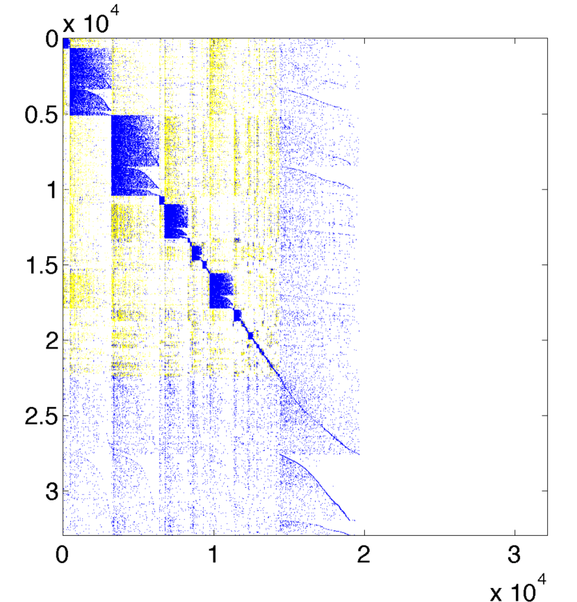
(a) $EN$-harvesting

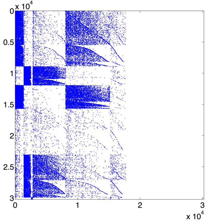
(b) DI-SIM

Figure 4: (a): Cora citation network arranged by directional communities. The rows and columns are arranged by the source parts and the terminal parts of the 78 $ADC^{EN}$s and remaining nodes are appended at the end of rows and columns. (b): Cora citation network with rows and columns reordered by the result of the DI-SIM algorithm.

Visualization of the communities detected by harvesting algorithms is not straightforward due to the possibility of multiple memberships. The rows and columns are arranged by the source parts and the terminal parts of the detected $ADC$s and the remaining nodes are appended at the end of rows and columns. Internal edges of $ADC$ appear as blue blocks in the diagonal. Meanwhile, blue dots outside the blocks are the edges that are not harvested in the algorithm. Yellow dots are the internal edges that reappear because of the multiple membership of nodes.

The result from the DI-SIM algorithm is summarized by the adjacency matrix with rows and columns reordered by the two separate partitions (Figure 4(b)). The adjacency matrix rearranged by the communities of Infomap is shown in Figure 1(a).

The communities detected by harvesting algorithms reveal different representation of the underlying structure than other two methods. First, harvesting algorithms capture asymmetric nature of the communities in the citation network. The symmetric assumption of Infomap yields tiny communities that are less significant. Second, the proposed algorithms reveal correspondence between source nodes and terminal nodes while DI-SIM treats them separately.

5.1.2 Correspondence between Communities and Manual Categories

The manually assigned categories of papers (Table 2) in Cora citation network provided us with extra information to validate the quality of the detected communities. The sizes of category span a large range, from $582$ papers in Information Retrieval to $10784$ papers in Artificial Intelligence. Given the categories, we calculate the conductance value of each category to see the quality of a category as a community. Those values are greater than those of $ADC^{L_{0}}$s in general (See Table 4 in Appendix D).

Table 2: List of ten fields of Computer Science and their number of papers and conductance.

Number	Name of Major Field of CS	Number of Papers	$\phi$
1	Artificial Intelligence	10784	0.1568
2	Data Structures Algorithms and Theory	3104	0.3854
3	Databases	1261	0.3429
4	Encryption and Compression	1181	0.4096
5	Hardware and Architecture	1207	0.4762
6	Human Computer Interaction	1651	0.4527
7	Information Retrieval	582	0.3932
8	Networking	1561	0.3686
9	Operating Systems	2580	0.3736
10	Programming	3972	0.3178

Table 3: Number of papers in the first six approximated directional components of $L_{0}$-harvesting for each category.

	AI	DSAT	DB	EC	HA	HCI	IR	Net	OS	Prog
1	106	199	56	18	255	17	0	55	900	1779
2	2741	68	30	9	8	28	63	17	34	75
3	13	12	25	115	11	307	18	936	232	34
4	727	124	8	102	12	577	10	6	22	21
5	284	83	803	9	9	17	66	14	16	80
6	149	452	3	239	12	0	2	3	9	6

We investigate the correspondence between the detected communities and the manually assigned categories. We consider the largest $6$ communities of $L_{0}$-harvesting since they show significantly lower conductance than the rest of communities. The comparison is reported in Table 3. The six largest communities $ADC^{L_{0}}_{1},\ldots,ADC^{L_{0}}_{6}$ show significant correspondence to the major-fields of CS. For example, $ADC^{L_{0}}_{1}$ mainly consists of two fields, operating system (OS) and programing (Prog), also $ADC^{L_{0}}_{2}$ is dominated by papers from artificial intelligence (AI).

Remaining smaller communities showed high precision and low recall with respect to the major-fields. Some of them seem to be fragments that are not strongly connected to bigger communities. However, we found that many of them showed correspondence to sub-fields embedded in major-fields. For example, many of the small communities are related to AI category and they represent interactions in sub-fields of AI.

The communities detected by harvesting algorithms meet our expectations regarding the manual categories. The detected communities revealed densely connected papers that can be considered as a core part within a manual category. We also suspect a possible hierarchical community structure within the large communities and we leave investigations along this direction in our future work.

5.2 Harvesting Algorithms in a Large Social Network

The massive size of modern network data, more than millions of nodes in a network, demands scalable algorithms. Many community detection algorithms that search for optimal partition of nodes do not scale well. On the other hand, harvesting algorithms detect a community at a time based on a locally defined quality measure. In this experiment, we test our harvesting algorithms on a social network that is large and highly asymmetric.

We analyze a social network dataset of Tencent Weibo, a micro-blogging website of China. Users in this network may subscribe to news feeds from others and each subscription is represented as a directed edge between users. This network contains $1944589$ non-zero degree nodes and $50655143$ edges, which leads to an average out-degree $25$. The social network is highly asymmetric and it has only $0.2\%$ of symmetric links.

The computation time to harvest $1000$ $ADC^{L_{0}}$ was about $12$ hours and that of harvesting $463$ $ADC^{EN}$ was around $6$ hours. The algorithms are run in a linux machine (2$\times$ Six Core Xeon X5650 / 2.66GHz / 48GB). The settings of the algorithms can be found in Appendix E.

To check the quality of harvested communities, we report the conductance values, $\phi$, along with the size of $ADC$s (Figure 5(a)). $L_{0}$-harvesting is better at detecting larger communities while $EN$-harvesting tends to detect smaller communities and a few very large communities. We also display the $1000$ largest communities obtained by Infomap, whose directional conductances are computed under the symmetric constraint $S=T$. The communities found under the symmetric assumption show relatively higher conductance values. Additionally, we verified that good communities are relatively small ($\sim 200$) in such huge social networks, as reported in Leskovec et al. (2008).

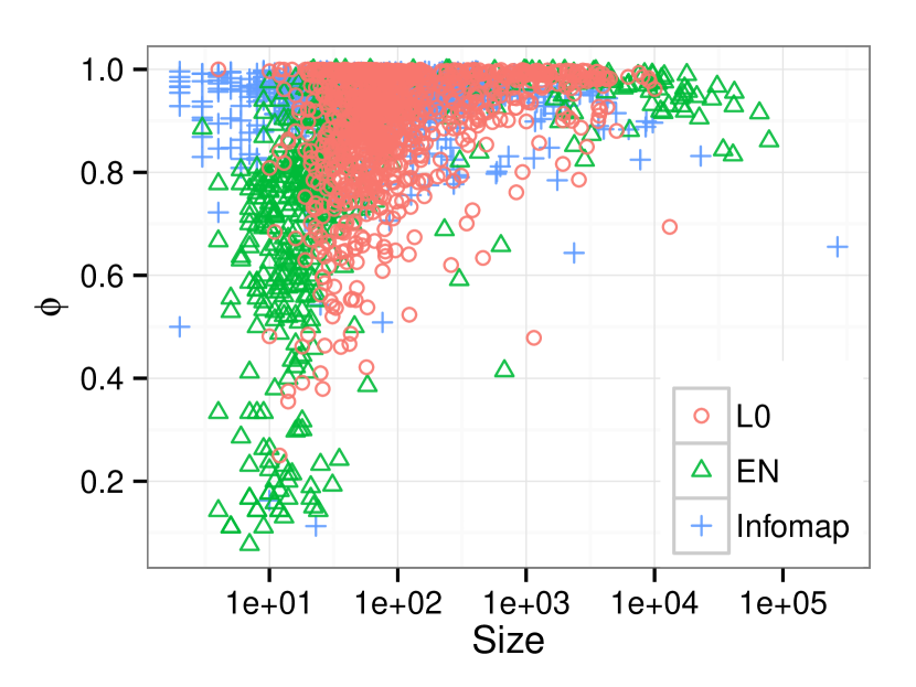
(a)

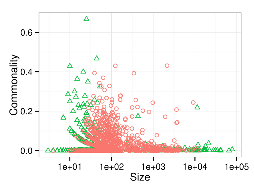
(b)

Figure 5: (a) Scatter plot of size of communities and directional conductance in a social network. (b) Scatter plot of size of communities and commonality.

The directional communities detected by harvesting algorithms show high asymmetricity. We investigate the asymmetricity of a community by looking at the ratio of members that are common in both parts. We define Commonality of a $ADC$ as the Jaccard similarity coefficient of the two parts (the ratio of the number of common nodes to the total number of nodes in the union of the two parts). Figure 5(b) shows that most detected communities are low in the commonality except some of small communities. Further inspection showed that the asymmetric communities are mostly formed by few popular terminal nodes (authorities) and large number of source nodes (normal users). This observation highlights the need of considering asymmetric directional communities in social networks.

6 Conclusions and Discussion

In this paper, we found that integrating two different roles of nodes is critical in characterizing a community of a directed network. We introduced a new notion of community, directional communities, that is capable of discerning the two different roles of each node in a community.

We proposed two regularized SVD based harvesting algorithms that sequentially identify directional communities. The regularized SVD method is linearly scalable to the number of edges in the network. The $L_{0}$-harvesting algorithm showed good performance even in networks having low average-degree. Meanwhile the $EN$-harvesting algorithm excelled in detecting relatively small and dense communities.

We believe directional communities enable genuine analysis on community structures in highly asymmetric directed networks of real applications. Also, the simplicity of harvesting algorithms, only relying on matrix multiplication and thresholding of vectors, leads to further improvement of the algorithm through parallel and distributed computing.

Appendix A Algorithm for Finding Directional Components

This section presents a simple searching algorithm for finding directional components that is introduced in Section 2.1.

Algorithm 3 Decompose a directed graph into directional components

1:${\cal G}=({\cal V},{\cal E}),k=1$

2:repeat

3:     $S=\emptyset,T=\emptyset$

4:     Add a source node $s\in{\cal V}$ whose out-degree is non-zero in ${\cal E}$ into the set $S$.

5:     repeat

6:         Find $E_{t}=\{e\in{\cal E}|v^{s}(e)\in S\}$.

7:         $T\leftarrow T\cup\{v^{t}(e)|e\in E_{t}\}$

8:         ${\cal E}\leftarrow{\cal E}-E_{t}$

9:         Find $E_{s}=\{e\in{\cal E}|v^{t}(e)\in T\}$

10:         $S\leftarrow S\cup\{v^{s}(e)|e\in E_{s}\}$

11:         ${\cal E}\leftarrow{\cal E}-E_{s}$

12:     until  $E_{t}=E_{s}=\emptyset$

13:     $DC_{k}\leftarrow(S,T)$

14:     $k\leftarrow k+1$

15:until ${\cal E}$ is empty.

16:return $DC_{1},\ldots,DC_{k}$

Appendix B PROOFS FOR REGULARIZED SVD ALGORITHMS

We presents the proofs of propositions of the main article.

Even though we assumed zero-one weights of edges in the main article, following proofs are also true for non-negative weights of edges. We denote the principal singular value of a matrix $X$ by $\sigma_{1}(X)$.

Proof of Proposition 3.1

Proof.

For notational convenience, here, $\mathbf{u}(v_{i})$ is shortened to $u_{i}$ and $\mathbf{v}(v_{j})$ is shortened to $v_{j}$. We show that $\phi_{\eta=0}(C(S,T))=\sum_{i,j}W_{ij}\left(\frac{u_{i}}{\sqrt{d_{r,i}}}-\frac{v_{j}}{\sqrt{d_{c,j}}}\right)^{2}$ and at the same time $\sum_{i,j}W_{ij}\left(\frac{u_{i}}{\sqrt{d_{r,i}}}-\frac{v_{j}}{\sqrt{d_{c,j}}}\right)^{2}=1-2\mathbf{u}^{t}Q\mathbf{v}$

$$\sum_{i,j}W_{ij}\left(\frac{u_{i}}{\sqrt{d_{r,i}}}-\frac{v_{j}}{\sqrt{d_{c,j}}}\right)^{2}={} \sum_{i\in S,j\in\bar{T}}W_{ij}\left(\frac{1}{\sqrt{\text{Vol}(S)+\text{Vol}(T)}}\right)^{2}+$$

$$\sum_{i\in\bar{S},j\in T}W_{ij}\left(\frac{1}{\sqrt{\text{Vol}(S)+\text{Vol}(T)}}\right)^{2}$$

$$={} \frac{\mbox{d-Cut}(C(S,T),C(\bar{S},\bar{T}))}{\text{Vol}(S)+\text{Vol}(T)}$$

and on the other hand,

$$\sum_{i,j}W_{ij}\left(\frac{u_{i}}{\sqrt{d_{r,i}}}-\frac{v_{j}}{\sqrt{d_{c,j}}}\right)^{2}={} \sum_{i,j}W_{ij}(\frac{u_{i}^{2}}{d_{r,i}}+\frac{v_{j}^{2}}{d_{c,j}}-\frac{2u_{i}v_{j}}{\sqrt{d_{r,i}d_{c,j}}})$$

$$={} \sum_{i}u_{i}^{2}+\sum_{j}v_{j}^{2}-2\sum_{i,j}W_{ij}\frac{u_{i}v_{j}}{\sqrt{d_{r,i}d_{c,j}}}$$

$$={} \mathbf{u}^{t}\mathbf{u}+\mathbf{v}^{t}\mathbf{v}-2\mathbf{u}^{t}Q\mathbf{v}$$

$$={} 1-2\mathbf{u}^{t}Q\mathbf{v}$$

The last equality holds by definition $\text{Vol}(S)=\sum_{i\in S}d_{r,i},\text{Vol}(T)=\sum_{j\in T}d_{c,j}$.

∎

Proof of Proposition 3.2

Proof.

Notice that we can modify the adjacency matrix $W$ by removing zero rows and zero columns without loss of generality. The modified matrix is denoted by $E\in\mathbb{R}^{|{\cal S}|\times|{\cal T}|}$, where ${\cal S}$ is the set of source nodes whose out-degree is non-zero and ${\cal T}$ is the set of terminal nodes whose in-degree is non-zero. The singular vectors of $W$ can be obtained by padding zeros back to the singular vectors of $E$.

We introduce a bipartite graph expression of a directed graph that is also considered in Zhou, Schölkopf and Hofmann (2005); Guimerà, Sales-Pardo and Amaral (2007). The bipartite graph converted from a directed graph ${\cal G=(V,E)}$ is ${\cal G}_{B}=({\cal S},{\cal T},{\cal L})$, where ${\cal S}$ is the set of source nodes and ${\cal T}$ is the set of terminal nodes and ${\cal L}$ is the set of undirected edges, $\{(v^{s}(e),v^{t}(e)),e\in{\cal E}\}$. The adjacency matrix of ${\cal G}_{B}$, $A$, is

$$A=\left[\begin{array}[]{ccc}0&E\\ E^{t}&0\end{array}\right].$$

This proof has two steps,

1. Show that a directional component of ${\cal G}$ is equivalent to a connected component of ${\cal G}_{B}$.

2. Use the relationship between the spectrum of Laplacian and connected components in an undirected graph to show the proposition.

First, let us show that a directional component ($DC$) in ${\cal G}$ is a connected component ($C$) in ${\cal G}_{B}$ by examining the connectivity and maximality conditions:

• Connectivity: First, any $(s,t),s\in{\cal{S}},t\in{\cal T}$ are connected in ${\cal G}_{B}$ by the D-connectivity, $s\leadsto t$. Second, any $(s_{1},s_{2}),s_{1}\in{\cal{S}},s_{2}\in{\cal S}$ are connected in ${\cal G}_{B}$ since there exists a common terminal node $t\in{\cal T}$ such that $s_{1}\leadsto t$ and $s_{2}\leadsto t$. And any $(t_{1},t_{2}),t_{1}\in{\cal T},t_{2}\in{\cal T}$ are connected in ${\cal G}_{B}$ for the existence of a common source node.

• Maximality: Assume that there exists a node that is connected to $C$ but not a member of $DC$. Then there should be a directed edge starting from the node or ended at the node in ${\cal G}$. In either case the node is a member of $DC$. It contradicts to the maximality of $DC$. Thus there is no such node.

Similarly, we show that a connected component $C$ in ${\cal G}_{B}$ is a directional component $DC$ in ${\cal G}$. Any pair of nodes $(s,t),s\in{\cal S},t\in{\cal T}$ is D-connected in ${\cal G}$ by the connectivity in ${\cal G}_{B}$. Maximality for a directional component is again obtained by using the maximality of $C$.

For the second step, we apply the proposition 4 of Von Luxburg (2007) that shows us the equivalence between the number of connected components of an undirected graph and the multiplicity of the zero eigenvalue of graph Laplacian matrix of the undirected graph. Let $L_{sym}$ be a normalized graph Laplacian of $A$, which is defined by

$$L_{sym}=I-Q_{A},$$

where,

$$Q_{A} =D_{A}^{-\frac{1}{2}}AD_{A}^{-\frac{1}{2}}$$

$$=\left[\begin{array}[]{ccc}0&Q\\ Q^{t}&0\end{array}\right]$$ (B.3)

and $D_{A}$ is the diagonal matrix of the row sums of $A$ and it is equal to

$$D_{A}=\left[\begin{array}[]{ccc}D_{r}&0\\ 0&D_{c}\end{array}\right].$$

The proposition 4 of Von Luxburg (2007) says that the multiplicity $K$ of the eigenvalue zero of $L_{sym}$ is equal to the number of connected components in the undirected graph corresponding to $A$ and the eigenspace of zero is spanned by the vectors $\{D_{A}^{\frac{1}{2}}\mathbf{1}_{C_{k}},k=1,\dots,K\}$, where $\mathbf{1}_{C_{k}}$ is the indicator vector for $k$th connected component.

By the definition of $L_{sym}$, if $\lambda$ is an eigenvalue of $L_{sym}$ then $1-\lambda$ is an eigenvalue of $Q_{A}$. It follows that the eigenvalue zero of $L_{sym}$ corresponds to the eigenvalue one of $Q_{A}$. In fact, one is the principal eigenvalue of $Q_{A}$ because the eigenvalue zero is the smallest eigenvalue of $L_{sym}$ which is a non-negative definite matrix.

By the standard result of the eigenvalues of $Q_{A}$ and the singular values of $Q$ (see Horn and Johnson, 1994, chap. 3), the principal singular value of $Q$ is the principal eigenvalue of $Q_{A}$, which is one. A vector $D_{A}^{\frac{1}{2}}\mathbf{1}_{C_{k}}$ can be broken into two vectors $D_{r}^{\frac{1}{2}}\mathbf{1}_{S_{k}}\in\mathbb{R}^{|{\cal{S}}|},D_{c}^{\frac{1}{2}}\mathbf{1}_{T_{k}}\in\mathbb{R}^{|{\cal T}|}$, where $D_{r}^{\frac{1}{2}}\mathbf{1}_{S_{k}}$ is the first $|{\cal{S}}|$ entries of $D_{A}^{\frac{1}{2}}\mathbf{1}_{C_{k}}$ and $D_{c}^{\frac{1}{2}}\mathbf{1}_{T_{k}}$ is the last $|{\cal T}|$ entries of $D_{A}^{\frac{1}{2}}\mathbf{1}_{C_{k}}$. By (B), the two vectors satisfy

$$\begin{cases}D_{r}^{\frac{1}{2}}\mathbf{1}_{S_{k}}&=QD_{c}^{\frac{1}{2}}\mathbf{1}_{T_{k}}\\ D_{c}^{\frac{1}{2}}\mathbf{1}_{T_{k}}&=Q^{t}D_{r}^{\frac{1}{2}}\mathbf{1}_{S_{k}},\end{cases}$$

as one can find in Dhillon (2001). $\{D_{r}^{\frac{1}{2}}\mathbf{1}_{S_{k}},k=1,\dots,K\}$ is a set of orthogonal vectors since $S_{k}$’s are exclusive. The same argument holds for $\{D_{c}^{\frac{1}{2}}\mathbf{1}_{T_{k}},k=1,\dots,K\}$. Thus, the pairs of vectors $\{(D_{r}^{\frac{1}{2}}\mathbf{1}_{S_{k}},D_{c}^{\frac{1}{2}}\mathbf{1}_{T_{k}}),k=1,\dots,K\}$ span the singular space of the singular value one of $Q$.

∎

Using the adjacency matrix expression of a directed graph, a directional component can be considered as a submatrix of a matrix. For a non-negative matrix $B$, we call a submatrix of $B$ a directional-component block if the submatrix is corresponding to a directional component of the directed graph generated from the weight matrix $B$.

We introduce a corollary of Proposition 3.2. This corollary is used in the proof of Theorem 3.3 later.

Corollary B.1.

For any submatrix of $Q$, say $Q_{s}$, the largest singular value of $Q_{s}$ is less than or equal to one ( $\sigma_{1}(Q_{s})\leq 1$), and the equality holds if and only if $Q_{s}$ includes directional-component blocks.

Proof.

First of all, we introduce a handy representation of a submatrix $Q_{s}\in\mathbb{R}^{k\times l}$. A submatrix of $Q$ is a matrix formed by selecting a subset of rows and columns of $Q$. We define a full-rank matrix, called a selection matrix, whose columns have only one non-zero entry with its value. Then, for any submatrix $Q_{s}$, we can find two selection matrices $M_{r}\in\mathbb{R}^{m\times k},M_{c}\in\mathbb{R}^{n\times l}$ such that

$$Q_{s}=M_{r}^{t}QM_{c},$$

according to the selected rows and columns.

The principal singular value of $Q_{s}$, $\sigma_{1}(Q_{s})$, is the solution of a optimization problem,

$$\max_{\mathbf{u}_{s},\mathbf{v}_{s}}\mathbf{u}_{s}^{t}Q_{s}\mathbf{v}_{s},\quad\|\mathbf{u}_{s}\|_{2}=1,\|\mathbf{v}_{s}\|_{2}=1.$$ (B.4)

with $\mathbf{u}_{s}\in\mathbb{R}^{k},\mathbf{v}_{s}\in\mathbb{R}^{l}$. By setting $\mathbf{u}=M_{r}\mathbf{u}_{s},\mathbf{v}=M_{c}\mathbf{v}_{s}$, we can see that (B.4) is equivalent to

$$\max_{\mathbf{u}_{s},\mathbf{v}_{s}}\mathbf{u}^{t}Q\mathbf{v},\quad\|\mathbf{u}\|_{2}=1,\|\mathbf{v}\|_{2}=1,\mathbf{u}=M_{r}\mathbf{u}_{s},\mathbf{v}=M_{c}\mathbf{v}_{s}$$ (B.5)

by $\|M_{r}\mathbf{u}_{s}\|_{2}=\|\mathbf{u}_{s}\|_{2},\|M_{c}\mathbf{v}_{s}\|_{2}=\|\mathbf{v}_{s}\|_{2}$. This optimization has constraints, $\mathbf{u}=M_{r}\mathbf{u}_{s},\mathbf{v}=M_{c}\mathbf{v}_{s}$, in addition to the formulation of the principal singular value of $Q$. Thus, $\sigma_{1}(Q_{s})\leq 1$ by Proposition 3.2.

Proposition 3.2 also tells us that $\sigma_{1}(Q_{s})=1$ if and only if $(u,v)\in\chi_{1}$ at the solution of (B.5), where $\chi_{1}\subset\mathbb{R}^{n+m}$ is the principal singular space of $Q$. Thus, it is clear that $\sigma_{1}(Q_{s})=1$ if and only if $\chi_{1}\cap\chi_{(M)}\neq\mathbf{0}$, where,

$$\chi_{(M)}=\mbox{span}\{\{(M_{r,i},\mathbf{0}_{m})\}_{i=1,\ldots,k}\cup\{(\mathbf{0}_{n},M_{c,i})\}_{i=1,\ldots,l}\},$$

where $M_{r,i}$ is the $i$-th column vector of $M_{r}$.

Therefore it is enough to show that $\chi_{1}\cap\chi_{(M)}\neq\mathbf{0}$ if and only if $Q_{s}$ includes directional component blocks. We want to clarify that this statement is about the condition on $M_{r},M_{c}$, which is equivalent to the condition on the selected rows and columns of $Q$ for $Q_{s}$.

We start to show one direction by taking an non-zero vector $(u,v)\in\chi_{1}\cap\chi_{M}$. Since $(u,v)\in\chi_{1}$, $(u,v)$ should have non-zero entries at the same places of non-zero entries of $(\mathbf{1_{S_{k}}},\mathbf{1_{T_{k}}})$ for some $k$. $(u,v)$ also belongs to $\chi_{M}$, thus the span of the columns of $M_{r}$ have to include $\mathbf{1_{S_{k}}}$ and also the span of the columns of $M_{c}$ have to include $\mathbf{1_{T_{k}}}$. Therefore, we conclude that $Q_{s}$ includes $(S_{k},T_{k})$ and it is true for any $k$.

The other direction can be shown easily by setting $Q_{s}$ to include a $k$th directional component block of $Q$. Then, $(D_{r}^{\frac{1}{2}}\mathbf{1}_{S_{k}},D_{c}^{\frac{1}{2}}\mathbf{1}_{T_{k}})\in\chi_{1}\cap\chi_{M}$.

∎

Now we show the solution of an optimization problem,

$$\max_{\mathbf{u},\mathbf{v}}\,\mathbf{u}^{t}Q\mathbf{v}-\eta(\|\mathbf{u}\|_{0}+\omega\|\mathbf{v}\|_{0}),\qquad\|\mathbf{u}\|_{2}\leq 1,\quad\|\mathbf{v}\|_{2}\leq 1,$$ (B.6)

provides a D-connected directional community.

Proof of Theorem 3.3

Proof.

Given membership vectors $\mathbf{u},\mathbf{v}$ and the corresponding community $C(S,T)$, notice that $\|\mathbf{u}\|_{0}=|S|$ and $\|\mathbf{v}\|_{0}=|T|$. We obtain a matrix $Q(C(S,T))$ by setting the rows and columns of $Q$ that are not in $S,T$ to zero vectors. Then, (B.6) can be written as

$$\max_{S,T}\sigma_{1}(Q(C(S,T)))-\eta SZ_{\omega}(C(S,T))$$ (B.7)

Suppose a solution $C(S^{*},T^{*})$ of (B.7) is not D-connected and can be decomposed into several maximal D-connected communities within $C(S^{*},T^{*})$. Then $\sigma_{1}(Q(C(S^{*},T^{*})))$ is equal to the principal singular value of one of the D-connected communities. But the size of the D-connected community is smaller than the size of $C(S^{*},T^{*})$. Thus the objective function of (B.7) can be increased by the smaller D-connected community. This contradicts the supposition that $C(S^{*},T^{*})$ maximizes the objective function.

Since a directional component is maximal D-connected subgraph, any D-connected subgraph should be a subgraph of some directional component.

We prove the second claim. Corollary B.1 tells us that $\sigma_{1}(Q(DC_{1}))$ is equal to $1$ and that is one of the largest among $\{\sigma_{1}(Q(C(S,T)))|SZ_{\omega}(C(S,T))\geq SZ_{\omega}(DC_{1})\}$. Thus all $C(S,T)$ such that $SZ_{\omega}(C(S,T))>SZ_{\omega}(DC_{1})$ can not be a solution. We consider the condition of $\eta$ that satisfies

$$1-\eta SZ_{\omega}(DC_{1})<\sigma_{1}(Q(C(S,T)))-\eta SZ_{\omega}(C(S,T)),$$

for some $C(S,T)$ such that $SZ_{\omega}(C(S,T))<SZ_{\omega}(DC_{1})$. After an arrangement of above inequality, $\eta$ should satisfy

$$\eta>\frac{1-\sigma_{1}(Q(C(S,T)))}{SZ_{\omega}(DC_{1})-SZ_{\omega}(C(S,T))}.$$ (B.8)

$SZ_{\omega}(DC_{1})-SZ_{\omega}(C(S,T))>0$ by the condition of $C(S,T)$ and $1-\sigma_{1}(Q(C(S,T)))>0$ by Corollary B.1, thus taking minimum over the possible communities finishes the proof. ∎

We provide a toy example illustrating how the regularized SVD can detect the smallest directional component. The left panel of Figure 6(a) shows the adjacency matrix of a network with ten nodes. The network has two directional components with different sizes. The parameter $\omega$ in defining the size of communities is set to $1.1$. We randomly select two subsets $(S,T)$ of nodes to generate a submatrix $Q(C(S,T))$ from the full graph Laplacian matrix $Q$. Consider $S,T$ as indexes of rows and columns of $Q$ respectively. For each selected $Q(C(S,T))$, we calculate its principal singular value $\sigma_{1}(Q(C(S,T)))$ and its size $SZ_{\omega}(C(S,T))$. In addition to 500 randomly chosen sub-matrices, those two directional components are included as references.

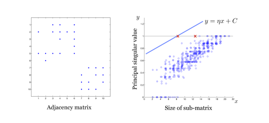
(a) No external edges

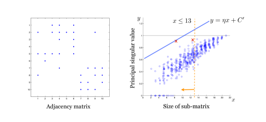
(b) After adding three external edges

Figure 6: Left panel of (a): The adjacency matrix of an example network having two directional components. Right panel of (a): Scatter plots of $SZ_{\omega}(C(S,T))$ and $\sigma_{1}(Q(C(S,T)))$. $Q(C(S,T))$ is a submatrix of the graph Laplacian matrix $Q$ derived from a directed graph having two directional components. Left panel of (b): The adjacency matrix of the example network of Figure 6(a) after adding three external edges. Right panel of (b): Scatter plots of $SZ_{\omega}(C(S,T))$ and $\sigma_{1}(Q(C(S,T)))$. $Q(C(S,T))$ is a submatrix of the graph Laplacian matrix $Q$ derived from the directed graph corrupted by external edges.

The right panel of Figure 6(a) show paired values $(SZ_{\omega}(C(S,T)),\sigma_{1}(Q(C(S,T))))$, with o, for each sampled submatrix $Q(C(S,T))$, and those two directional components are marked as Xs. Let us denote the value of objective function in (B.6) as $C$. This figure shows that there exist a line with slope $\eta>0$ whose intercept $C$ is maximized at the point corresponding to the smallest directional component as Theorem 3.3 describes. Therefore, the optimization (B.6) leads to identification of the smaller of the two directional components in this network. To summarize the result, both Proposition 3.2 and the example show that directional components, if there is any, can be identified sequentially by $L_{0}$ regularized SVD approach.

Recall that we encountered the problem that the small number of external edges connect small directional communities together as one large directional component. The root of the problem is the too strict requirement on finding exact directional components, the maximal set of node satisfying D-connectivity. The $L_{0}$ regularized SVD limits the number of non-zero entries of the singular vectors, so it may find a community that is smaller and almost separated from other communities.

To illustrate the advantage of the regularized approach, we add three external edges in the example. As a result, those two directional components merge together as one, as shown in the left panel of Figure 6(b). The right panel of Figure 6(b) plots paired values $(SZ_{\omega}(S,T),\sigma_{1}(Q(C(S,T))))$ of the same 500 pairs of $(S,T)$ shown in Figure 6(a). The principal singular values of two true directional components ( X marks) have decreased because of the added external edges, but the line with the same slope is still capable of identifying the original directional component. In addition to the argument of approximately minimizing penalized directional conductance, this example shows that the regularized SVD may capture smaller communities that are embedded in a directional component.

Proof of Proposition 3.4

Proof.

For a fixed number of non-zero entries $\|\mathbf{u}\|_{0}=l$, $\max_{\|\mathbf{u}\|_{2}\leq 1}\mathbf{u}^{t}\mathbf{z}$ is obtained when $\mathbf{u}={\mathbf{z}^{h}_{l}}/{\|\mathbf{z}^{h}_{l}\|_{2}}$. Thus the objective function (3.8) can be written as

$$F(l)=\|\mathbf{z}^{h}_{l}\|_{2}-\rho\,l.$$

Now we maximize $F(l)$ over $l$. Notice that $\|\mathbf{z}^{h}_{l}\|_{2}$ increases monotonically as $l$ increases. The value of $F(l)$ keeps increasing until

$$\sqrt{\|\mathbf{z}^{h}_{l}\|_{2}^{2}+|z|_{(l+1)}^{2}}-\|\mathbf{z}^{h}_{l}\|_{2}\leq\rho,$$

which is equivalent to (3.9). After $l$ goes beyond this point, $F(l)$ starts to decrease and keeps decreasing because $|z|^{2}_{(l)}$ decreases and $\|\mathbf{z}^{h}_{l}\|_{2}$ increases. Therefore, the solution to (3.8) is obtained at the minimum $l$ that satisfies (3.9). ∎

We begin to show an optimization problem,

$$\max_{\mathbf{u}}\mathbf{u}^{t}\mathbf{z},\quad\mbox{subject to }\quad(1-\alpha)\|\mathbf{u}\|^{2}_{2}+\alpha\|\mathbf{u}\|_{1}\leq c_{1},$$ (B.9)

can be solved by soft-thresholding. First, we introduce a definition.

Definition B.2.

3.5. For a vector $\mathbf{z}=(z_{1},\ldots,z_{n})^{\prime}\in\mathbb{R}^{n}$, recall the $l$-th largest absolute value of $\mathbf{z}$ was defined as ${|z|}_{(l)}$. We define

$$G_{\mathbf{z}}(x) =\frac{1}{4x^{2}}\sum_{i=1}^{k(x)-1}(|z|_{(i)}-x)^{2}+\frac{1}{2x}\sum_{i=1}^{k(x)-1}(|z|_{(i)}-x)$$ (B.10)

where $k(x)\in\{1,\dots,n+1\}$ satisfies $|z|_{(k(x))}\leq x<|z|_{(k(x)-1)}$ and define $|z|_{(n+1)}=0$.

Proof of Proposition 3.6

Proof.

The first part of this proof resembles the proof of Lemma 2.2 of Witten, Tibshirani and Hastie (2009). Express the objective function and the constraints by using a Lagrangian multiplier,

$$\min_{\mathbf{u},\lambda} -\mathbf{u}^{t}\mathbf{z}+\lambda((1-\alpha)\|\mathbf{u}\|_{2}^{2}+\alpha\|\mathbf{u}\|_{1}).$$ (B.11)

Then, differentiate the objective function in (B.11) by $\mathbf{u}$ and set it to zero,

$$-\mathbf{z}+\lambda(2(1-\alpha)\mathbf{u}+\alpha\Gamma)=0,$$

where $\Gamma_{i}=\mbox{sign}(u_{i})$ if $u_{i}\not=0$, otherwise $\Gamma_{i}\in[-1,1]$. The Karush-Kuhn-Tucker (KKT) conditions require $\lambda((1-\alpha)\|\mathbf{u}\|_{2}^{2}+\alpha\|\mathbf{u}\|_{1}-c_{1})=0$. If $\lambda>0$, the solution is

$$\hat{\mathbf{u}}=\frac{S(\mathbf{z},\lambda\alpha)}{2\lambda(1-\alpha)}.$$

$\lambda$ can be zero, if the solution is not on the boundary of the constraint. But it does not happen unless $\mathbf{z}$ is a zero vector. Thus, $\lambda>0$ is chosen so that $\hat{\mathbf{u}}$ satisfies the KKT condition.

$$(1-\alpha)\left\|\frac{S(\mathbf{z},\lambda\alpha)}{2\lambda(1-\alpha)}\right\|_{2}^{2}+\alpha\left\|\frac{S(\mathbf{z},\lambda\alpha)}{2\lambda(1-\alpha)}\right\|_{1}=c_{1}$$

$$\Rightarrow \frac{1}{(2\lambda)^{2}(1-\alpha)}\sum_{i=1}^{k-1}(|{z}|_{(i)}-\lambda\alpha)^{2}+\frac{\alpha}{2\lambda(1-\alpha)}\sum_{i=1}^{k-1}(|{z}|_{(i)}-\lambda\alpha)=c_{1}$$ (B.12)

where $k$ satisfies $|{z}|_{(k)}\leq\lambda\alpha<|{z}|_{(k-1)}$. Denote the threshold level $d=\lambda\alpha$, then (B) becomes

$$\left(\frac{1}{4d^{2}}\sum_{i=1}^{k-1}(|{z}|_{(i)}-d)^{2}+\frac{1}{2d}\sum_{i=1}^{k-1}(|{z}|_{(i)}-d)\right)=c_{1}\frac{1-\alpha}{\alpha^{2}},$$ (B.13)

where $k$ satisfies $|{z}|_{(k)}\leq d<|{z}|_{(k-1)}$. Using Lemma B.3, one can determine the threshold level $d$ of (B.13) by setting $\mathbf{z}$ and $c=c_{1}\frac{1-\alpha}{\alpha^{2}}$. Even though the value of $\lambda$ is not required for the solution, we present it for the record.

$$\lambda=\frac{1}{\alpha}\left(\frac{\sum_{i=1}^{\hat{k}}|{z}|_{(i)}^{2}}{4(c_{1}\frac{1-\alpha}{\alpha^{2}})+\hat{k}}\right)^{\frac{1}{2}}.$$

∎

Now, we show how to obtain the threshold level in Proposition 3.6.

Lemma B.3.

The solution of the equation $G_{\mathbf{z}}(d)=c$ for given $c>0$ is

$$d=\left(\frac{\sum_{i=1}^{\hat{k}}|z|_{(i)}^{2}}{4c+\hat{k}}\right)^{\frac{1}{2}},$$ (B.14)

where $\hat{k}$ is a positive integer in $\{1,2,\dots,n\}$ that satisfies $G_{\mathbf{z}}(|z|_{(\hat{k})})\leq c,G_{\mathbf{z}}(|z|_{(\hat{k}+1)})>c$.

Proof.

For the first step, we show that $G_{\mathbf{z}}(\cdot)$ is a monotone decreasing function, that is, if $d_{1}>d_{2}$, then $G_{\mathbf{z}}(d_{1})<G_{\mathbf{z}}(d_{2})$. The first term of (B.10) is monotone decreasing of $d$ because

$$\frac{1}{4d_{2}^{2}}\sum_{i=1}^{k(d_{2})-1}(|z|_{(i)}-d_{2})^{2} >\frac{1}{4d_{1}^{2}}\sum_{i=1}^{k(d_{1})-1}(|z|_{(i)}-d_{2})^{2}$$

$$>\frac{1}{4d_{1}^{2}}\sum_{i=1}^{k(d_{1})-1}(|z|_{(i)}-d_{1})^{2}.$$

The first inequality comes from the fact that $k(d_{2})\leq k(d_{1})$ and $d_{1}>d_{2}$. The second inequality comes from $d_{1}>d_{2}$. The second term of (B.10) can be done in the similar way and the desired result is obtained.

For the second step, we find the approximated solution of $d$ from the set of $\{|z|_{(i)}\}_{i=1\ldots n}$. By plugging in $|z|_{(i)}$ to $d$ in the increasing order of $i$, we can find $\hat{k}$ such that $G_{\mathbf{z}}(|z|_{(\hat{k})})\leq c$, $G_{\mathbf{z}}(|z|_{(\hat{k}+1)})>c$ by the monotonicity of $G_{\mathbf{z}}(\cdot)$ and being $c$ in the range of $G_{\mathbf{z}}(\cdot)$. This computation can be done efficiently by computing two cumulative sums, $\sum_{i}^{k}|z|_{(i)}^{2}$ and $\sum_{i}^{k}|z|_{(i)}$, in the increasing order of $k$ until $\hat{k}$ is obtained. An algorithm for finding $\hat{k}$ in this Lemma is provided in Algorithm 4.

Algorithm 4 Find $\hat{k}$ such that $G_{\mathbf{z}}(|z|_{(\hat{k})})\leq c$, $G_{\mathbf{z}}(|z|_{(\hat{k}+1)})>c$

1:$(z_{1}\geq z_{2}\geq,\dots,\geq z_{n}),c>0$

2:initialize $S_{1}\leftarrow 0,S_{2}\leftarrow 0,\hat{k}\leftarrow 2$

3:for $k=2:n$ do

4:     $S_{1}\leftarrow S_{1}+z_{k-1}$

5:     $S_{2}\leftarrow S_{2}+z_{k-1}^{2}$

6:     $G_{k}=\frac{1}{4z_{k}^{2}}(S_{2}-2z_{k}S_{1}+(k-1)z_{k}^{2})+\frac{1}{2z_{k}}(S_{1}-(k-1)z_{k})$

7:     if $G_{k}>c$ then

8:         $\hat{k}\leftarrow k-1$

9:         return $\hat{k}$

10:     end if

11:end for

12:if $G_{k}\leq c$ then

13:     $\hat{k}\leftarrow n$

14:     return $\hat{k}$

15:end if

In the second step, we already know that $|z|_{(\hat{k}+1)}<d\leq|z|_{(\hat{k})}$ which means $k=\hat{k}$ fixed now. Therefore solving a quadratic equation of $d$,

$$\frac{1}{4d^{2}}\sum_{i=1}^{\hat{k}}(|z|_{(i)}-d)^{2}+\frac{1}{2d}\sum_{i=1}^{\hat{k}}(|z|_{(i)}-d)=c$$

determines the solution $d$. By the quadratic formula, the solution is

$$d=\left(\frac{\sum_{i=1}^{\hat{k}}|z|_{(i)}^{2}}{4c+\hat{k}}\right)^{\frac{1}{2}},$$

knowing that $d>0$. ∎

Appendix C Algorithm Settings for Simulation

The true number of communities $N_{C}$ is provided for DI-SIM algorithm. We compute the first $N_{C}$ singular vectors of $Q$ and apply the k-means algorithm with $N_{C}$ clusters on the left and right singular vectors separately. We run k-means algorithm with $100$ random initializations and the one minimizing the within-cluster sums of point-to-cluster-centroid distances is reported as the final result. To obtain directional communities out of the two separate partitions, we match the source part and the terminal part by the largest common edges.

We use Infomap implementation Infomap-0.11.5 available at http://www.mapequation.org. The default settings are used except for the options for directed links (--directed) and two-level partition of the network (--two-level). 100 repetitions (--num-trials) are used to pick the best solution.

Harvesting algorithms are initialized with $v_{0}$ being the node of largest in-degree at each harvesting. The sparsity levels for source part and terminal part are set to the same value, $\omega=1$ and $\alpha=\beta$. The range of them are determined so that the detected communities are sized roughly $SZ_{\omega=1}(C)\in(20,400)$, More specifically, the grid of sparsity levels for $L_{0}$ penalty, $\eta$, contains $10$ points in $\{\exp(-k):k=6+i(5/10),i=1,\ldots,10\}$ and the grid of sparsity levels for $EN$ penalty, $\alpha$, includes $10$ points in $\{\frac{1}{1+\exp(k)}:k=1+i(3.7/10),i=1,\ldots,10\}$. Those non-linear grids are adapted for more constant change of the size of candidate communities. Early stopping parameters are set to $s_{p}=1.5$ and $s_{l}=0.6$. The harvesting algorithm continues until the number of harvested communities reaches the true number of communities or there is no more edge left.

Appendix D Communities in Cora Citation Network

Here we present details of $ADC$s found in Cora Citation Network. Table 4 shows four summaries of $20$ $ADC^{L_{0}}$ and $ADC^{EN}$ ordered by the size. $|S|$ and $|T|$ are the number of source nodes and terminal nodes, $|E|$ is the number of edges in the community. $\phi$ is the value of directional conductance.

Also we provide a comparison between manual categories of papers and communities detected by four algorithms ($L_{0}$-harvesting: Table 5, $EN$-harvesting: Table 6, DI-SIM: Table 7) Those tables show the number of papers in manually assigned categories for each community.

Table 4: Summary of the largest $20$ $ADC$s of Cora citation network. $|S|$ is the number of source nodes and $|T|$ is the number of terminal nodes and $|E|$ is the number of edges. $\phi$ stands for directional conductance.

Order	$|S|$	$|T|$	$|E|$	$\phi$
1	3266	2321	21851	0.1500
2	2636	1886	12972	0.2244
3	1543	1128	8342	0.1724
4	1381	971	4690	0.2034
5	1270	919	6037	0.1910
6	803	512	3790	0.1271
7	694	480	4143	0.3638
8	577	485	2299	0.4906
9	573	447	2018	0.3070
10	583	361	2455	0.4363
11	539	368	2522	0.3033
12	503	403	1580	0.3588
13	587	278	1750	0.4666
14	479	251	1659	0.2909
15	390	278	1558	0.3031
16	368	233	938	0.4609
17	370	207	1007	0.3271
18	334	171	970	0.2416
19	291	207	1119	0.2312
20	226	154	672	0.4978

(a) First $20$ $ADC^{L_{0}}$.

Order	$|S|$	$|T|$	$|E|$	$\phi$
1	5319	3176	25428	0.2579
2	4458	2756	17137	0.2437
3	2309	1535	10422	0.2626
4	2254	1546	14539	0.2176
5	914	650	3127	0.3839
6	752	488	3219	0.3605
7	643	444	2522	0.4176
8	528	323	1561	0.3223
9	441	304	1487	0.3702
10	453	276	1602	0.2505
11	258	139	1504	0.2965
12	225	164	987	0.3794
13	245	116	1515	0.2070
14	195	130	558	0.3265
15	187	136	555	0.5642
16	187	132	629	0.2128
17	191	120	512	0.3706
18	162	94	512	0.2834
19	141	115	510	0.4501
20	168	80	430	0.2624

(b) First $20$ $ADC^{EN}$.

Table 5: Number of papers in the first twenty approximated directional components of $L_{0}$-harvesting for each category.

	AI	DSAT	DB	EC	HA	HCI	IR	Net	OS	Prog
1	106	199	56	18	255	17	0	55	900	1779
2	2741	68	30	9	8	28	63	17	34	75
3	13	12	25	115	11	307	18	936	232	34
4	727	124	8	102	12	577	10	6	22	21
5	284	83	803	9	9	17	66	14	16	80
6	149	452	3	239	12	0	2	3	9	6
7	16	40	95	19	94	32	7	50	347	96
8	40	90	14	14	32	11	0	112	254	157
9	283	184	0	8	29	19	1	3	32	37
10	18	38	30	13	2	28	0	27	355	127
11	651	1	0	2	1	1	24	0	0	4
12	524	7	3	1	0	22	73	1	2	22
13	543	23	1	3	2	1	45	0	9	31
14	492	4	10	8	8	2	1	0	0	3
15	427	11	0	8	0	1	3	0	3	3
16	104	6	23	3	3	187	12	0	13	110
17	21	9	3	307	3	8	2	20	40	22
18	20	66	2	0	221	0	0	26	6	15
19	243	14	0	7	15	1	0	1	12	34
20	292	1	1	3	0	5	7	0	0	0

Table 6: Number of papers in the first twenty approximated directional components of $EN$-harvesting for each category.

	AI	DSAT	DB	EC	HA	HCI	IR	Net	OS	Prog
1	573	341	649	184	175	396	83	449	1136	1817
2	4015	78	90	49	37	134	365	24	96	167
3	2218	39	56	25	9	43	49	88	61	92
4	80	238	42	11	214	17	1	71	891	809
5	214	583	62	21	42	62	2	70	32	44
6	25	18	5	78	6	97	9	587	62	15
7	708	12	11	13	13	5	3	0	2	8
8	186	186	11	12	31	6	0	6	23	52
9	75	37	103	0	7	0	0	0	6	293
10	15	31	0	394	4	2	2	28	38	6
11	0	1	2	18	0	38	0	192	23	0
12	26	8	1	2	0	0	0	0	1	220
13	76	132	1	37	1	0	0	0	4	2
14	95	30	0	0	0	120	0	1	1	4
15	16	14	173	7	4	5	6	2	12	15
16	169	33	0	0	0	8	0	0	2	2
17	99	9	0	6	0	126	0	0	1	0
18	5	9	1	11	135	1	1	3	0	15
19	0	1	2	1	4	0	0	8	98	49
20	13	3	0	0	136	0	0	3	3	5

Table 7: Number of papers in the source partition DI-SIM for each category.

	AI	DSAT	DB	EC	HA	HCI	IR	Net	OS	Prog
1	687	1084	723	575	571	416	71	750	1176	1933
2	28	4	0	0	0	0	0	0	1	0
3	4	0	0	0	0	0	0	0	0	0
4	2650	14	18	21	6	47	95	1	5	14
5	120	165	78	85	177	173	13	489	1023	1075
6	100	42	5	14	13	17	5	10	18	23
7	2509	1374	269	316	373	506	126	288	305	779
8	13	8	0	18	0	3	0	0	0	0
9	4658	406	167	149	64	485	272	20	50	148
10	15	7	1	3	3	4	0	3	2	0

Appendix E HARVESTING ALGORITHM SETTINGS FOR SOCIAL NETWORK DATA

The sparsity level parameters in the harvesting algorithms are designed to capture communities with the size in the range of $10$ to $100000$ approximately. The grid of sparsity parameter $\eta$ in $L_{0}$-harvesting is set as $\{\exp(-k):k=10+i(13/50),i=1,\ldots,50\}$ and the grid for $\alpha=\beta$ in $EN$-harvesting is set as $\{\frac{1}{1+\exp(k)};k=5+i(6/50),i=1,\ldots,50\}$. The early stopping method is applied with the parameters $s_{p}=1.1$ and $s_{l}=0.8$.

References

- Andersen, Chung and Lang (2007) {bincollection}[author] \bauthor\bsnmAndersen, \bfnmReid\binitsR., \bauthor\bsnmChung, \bfnmFan\binitsF. and \bauthor\bsnmLang, \bfnmKevin\binitsK. (\byear2007). \btitleLocal partitioning for directed graphs using PageRank. In \bbooktitleAlgorithms and Models for the Web-Graph \bpages166–178. \bpublisherSpringer. \endbibitem
- Andersen and Lang (2006) {binproceedings}[author] \bauthor\bsnmAndersen, \bfnmR.\binitsR. and \bauthor\bsnmLang, \bfnmK. J.\binitsK. J. (\byear2006). \btitleCommunities from seed sets. In \bbooktitleProceedings of the 15th international conference on World Wide Web \bpages223–232. \bpublisherACM. \endbibitem
- Arenas et al. (2007) {barticle}[author] \bauthor\bsnmArenas, \bfnmA.\binitsA., \bauthor\bsnmDuch, \bfnmJ.\binitsJ., \bauthor\bsnmFernández, \bfnmA.\binitsA. and \bauthor\bsnmGómez, \bfnmS.\binitsS. (\byear2007). \btitleSize reduction of complex networks preserving modularity. \bjournalNew Journal of Physics \bvolume9 \bpages176. \endbibitem
- Benzi, Estrada and Klymko (2012) {barticle}[author] \bauthor\bsnmBenzi, \bfnmMichele\binitsM., \bauthor\bsnmEstrada, \bfnmErnesto\binitsE. and \bauthor\bsnmKlymko, \bfnmChristine\binitsC. (\byear2012). \btitleRanking hubs and authorities using matrix functions. \bjournalLinear Algebra and its Applications. \endbibitem
- Boley, Ranjan and Zhang (2011) {barticle}[author] \bauthor\bsnmBoley, \bfnmDaniel\binitsD., \bauthor\bsnmRanjan, \bfnmGyan\binitsG. and \bauthor\bsnmZhang, \bfnmZhi-Li\binitsZ.-L. (\byear2011). \btitleCommute times for a directed graph using an asymmetric Laplacian. \bjournalLinear Algebra and its Applications \bvolume435 \bpages224–242. \endbibitem
- Capocci et al. (2005) {barticle}[author] \bauthor\bsnmCapocci, \bfnmA.\binitsA., \bauthor\bsnmServedio, \bfnmV. D. P.\binitsV. D. P., \bauthor\bsnmCaldarelli, \bfnmG.\binitsG. and \bauthor\bsnmColaiori, \bfnmF.\binitsF. (\byear2005). \btitleDetecting communities in large networks. \bjournalPhysica A: Statistical Mechanics and its Applications \bvolume352 \bpages669–676. \endbibitem
- Chung (2005) {barticle}[author] \bauthor\bsnmChung, \bfnmFan\binitsF. (\byear2005). \btitleLaplacians and the Cheeger inequality for directed graphs. \bjournalAnnals of Combinatorics \bvolume9 \bpages1–19. \endbibitem
- Clauset (2005) {barticle}[author] \bauthor\bsnmClauset, \bfnmA.\binitsA. (\byear2005). \btitleFinding local community structure in networks. \bjournalPhysical Review E \bvolume72 \bpages026132. \endbibitem
- Coscia, Giannotti and Pedreschi (2011) {barticle}[author] \bauthor\bsnmCoscia, \bfnmM.\binitsM., \bauthor\bsnmGiannotti, \bfnmF.\binitsF. and \bauthor\bsnmPedreschi, \bfnmD.\binitsD. (\byear2011). \btitleA classification for community discovery methods in complex networks. \bjournalStatistical Analy Data Mining. \endbibitem
- Danon et al. (2005) {barticle}[author] \bauthor\bsnmDanon, \bfnmL.\binitsL., \bauthor\bsnmDíaz-Guilera, \bfnmA.\binitsA., \bauthor\bsnmDuch, \bfnmJ.\binitsJ. and \bauthor\bsnmArenas, \bfnmA.\binitsA. (\byear2005). \btitleComparing community structure identification. \bjournalJournal of Statistical Mechanics: Theory and Experiment \bvolume2005 \bpagesP09008. \endbibitem
- d’Aspremont, Bach and Ghaoui (2008) {barticle}[author] \bauthor\bsnmd’Aspremont, \bfnmA.\binitsA., \bauthor\bsnmBach, \bfnmF.\binitsF. and \bauthor\bsnmGhaoui, \bfnmL. E.\binitsL. E. (\byear2008). \btitleOptimal solutions for sparse principal component analysis. \bjournalThe Journal of Machine Learning Research \bvolume9 \bpages1269–1294. \endbibitem
- Dhillon (2001) {binproceedings}[author] \bauthor\bsnmDhillon, \bfnmI. S.\binitsI. S. (\byear2001). \btitleCo-clustering documents and words using bipartite spectral graph partitioning. In \bbooktitleProceedings of the seventh ACM SIGKDD international conference on Knowledge discovery and data mining \bpages269–274. \bpublisherACM. \endbibitem
- Fortunato (2010) {barticle}[author] \bauthor\bsnmFortunato, \bfnmS.\binitsS. (\byear2010). \btitleCommunity detection in graphs. \bjournalPhysics Reports \bvolume486 \bpages75–174. \endbibitem
- Guimerà, Sales-Pardo and Amaral (2007) {barticle}[author] \bauthor\bsnmGuimerà, \bfnmR.\binitsR., \bauthor\bsnmSales-Pardo, \bfnmM.\binitsM. and \bauthor\bsnmAmaral, \bfnmL. A. N.\binitsL. A. N. (\byear2007). \btitleModule identification in bipartite and directed networks. \bjournalPhysical Review E \bvolume76 \bpages036102. \endbibitem
- Holland, Laskey and Leinhardt (1983) {barticle}[author] \bauthor\bsnmHolland, \bfnmP. W.\binitsP. W., \bauthor\bsnmLaskey, \bfnmK. B.\binitsK. B. and \bauthor\bsnmLeinhardt, \bfnmS.\binitsS. (\byear1983). \btitleStochastic blockmodels: first steps. \bjournalSocial networks \bvolume5 \bpages109–137. \endbibitem
- Horn and Johnson (1994) {bbook}[author] \bauthor\bsnmHorn, \bfnmR. A.\binitsR. A. and \bauthor\bsnmJohnson, \bfnmC. R.\binitsC. R. (\byear1994). \btitleTopics in Matrix Analysis. \bseriesTopics in Matrix Analysis. \bpublisherCambridge University Press. \endbibitem
- Kannan, Vempala and Vetta (2004) {barticle}[author] \bauthor\bsnmKannan, \bfnmRavi\binitsR., \bauthor\bsnmVempala, \bfnmSantosh\binitsS. and \bauthor\bsnmVetta, \bfnmAdrian\binitsA. (\byear2004). \btitleOn clusterings: Good, bad and spectral. \bjournalJournal of the ACM (JACM) \bvolume51 \bpages497–515. \endbibitem
- Kim and Shi (2013) {barticle}[author] \bauthor\bsnmKim, \bfnmSungmin\binitsS. and \bauthor\bsnmShi, \bfnmTao\binitsT. (\byear2013). \btitleScalable Spectral Algorithms for Community Detection in Directed Networks. \bjournalSubmitted. \endbibitem
- Kleinberg (1999) {barticle}[author] \bauthor\bsnmKleinberg, \bfnmJ. M.\binitsJ. M. (\byear1999). \btitleAuthoritative sources in a hyperlinked environment. \bjournalJournal of the ACM (JACM) \bvolume46 \bpages604–632. \endbibitem
- Lancichinetti, Fortunato and Radicchi (2008) {barticle}[author] \bauthor\bsnmLancichinetti, \bfnmA.\binitsA., \bauthor\bsnmFortunato, \bfnmS.\binitsS. and \bauthor\bsnmRadicchi, \bfnmF.\binitsF. (\byear2008). \btitleBenchmark graphs for testing community detection algorithms. \bjournalPhysical Review E \bvolume78. \endbibitem
- Lancichinetti and Fortunato (2009) {barticle}[author] \bauthor\bsnmLancichinetti, \bfnmA.\binitsA. and \bauthor\bsnmFortunato, \bfnmS.\binitsS. (\byear2009). \btitleCommunity detection algorithms: a comparative analysis. \bjournalPhysical Review E \bvolume80 \bpages056117. \endbibitem
- Lancichinetti, Fortunato and Kertész (2009) {barticle}[author] \bauthor\bsnmLancichinetti, \bfnmA.\binitsA., \bauthor\bsnmFortunato, \bfnmS.\binitsS. and \bauthor\bsnmKertész, \bfnmJ.\binitsJ. (\byear2009). \btitleDetecting the overlapping and hierarchical community structure in complex networks. \bjournalNew Journal of Physics \bvolume11 \bpages033015. \endbibitem
- Lee et al. (2010) {barticle}[author] \bauthor\bsnmLee, \bfnmM.\binitsM., \bauthor\bsnmShen, \bfnmH.\binitsH., \bauthor\bsnmHuang, \bfnmJ. Z.\binitsJ. Z. and \bauthor\bsnmMarron, \bfnmJS\binitsJ. (\byear2010). \btitleBiclustering via sparse singular value decomposition. \bjournalBiometrics \bvolume66 \bpages1087–1095. \endbibitem
- Leskovec et al. (2008) {binproceedings}[author] \bauthor\bsnmLeskovec, \bfnmJ.\binitsJ., \bauthor\bsnmLang, \bfnmK. J.\binitsK. J., \bauthor\bsnmDasgupta, \bfnmA.\binitsA. and \bauthor\bsnmMahoney, \bfnmM. W.\binitsM. W. (\byear2008). \btitleStatistical properties of community structure in large social and information networks. In \bbooktitleProceeding of the 17th international conference on World Wide Web \bpages695–704. \bpublisherACM. \endbibitem
- Meila and Pentney (2007) {binproceedings}[author] \bauthor\bsnmMeila, \bfnmMarina\binitsM. and \bauthor\bsnmPentney, \bfnmWilliam\binitsW. (\byear2007). \btitleClustering by weighted cuts in directed graphs. In \bbooktitleProceedings of the 7th SIAM International Conference on Data Mining \bpages135–144. \bpublisherCiteseer. \endbibitem
- Newman and Leicht (2007) {barticle}[author] \bauthor\bsnmNewman, \bfnmMark EJ\binitsM. E. and \bauthor\bsnmLeicht, \bfnmElizabeth A\binitsE. A. (\byear2007). \btitleMixture models and exploratory analysis in networks. \bjournalProceedings of the National Academy of Sciences \bvolume104 \bpages9564–9569. \endbibitem
- Rohe and Yu (2012) {barticle}[author] \bauthor\bsnmRohe, \bfnmK.\binitsK. and \bauthor\bsnmYu, \bfnmB.\binitsB. (\byear2012). \btitleCo-clustering for Directed Graphs; the Stochastic Co-Blockmodel and a Spectral Algorithm. \bjournalarXiv preprint arXiv:1204.2296. \endbibitem
- Rosvall, Axelsson and Bergstrom (2009) {barticle}[author] \bauthor\bsnmRosvall, \bfnmM.\binitsM., \bauthor\bsnmAxelsson, \bfnmD.\binitsD. and \bauthor\bsnmBergstrom, \bfnmC. T.\binitsC. T. (\byear2009). \btitleThe map equation. \bjournalThe European Physical Journal-Special Topics \bvolume178 \bpages13–23. \endbibitem
- Satuluri and Parthasarathy (2011) {binproceedings}[author] \bauthor\bsnmSatuluri, \bfnmV.\binitsV. and \bauthor\bsnmParthasarathy, \bfnmS.\binitsS. (\byear2011). \btitleSymmetrizations for clustering directed graphs. In \bbooktitleProceedings of the 14th International Conference on Extending Database Technology \bpages343–354. \bpublisherACM. \endbibitem
- Shen and Huang (2008) {barticle}[author] \bauthor\bsnmShen, \bfnmH.\binitsH. and \bauthor\bsnmHuang, \bfnmJ. Z.\binitsJ. Z. (\byear2008). \btitleSparse principal component analysis via regularized low rank matrix approximation. \bjournalJournal of multivariate analysis \bvolume99 \bpages1015–1034. \endbibitem
- Von Luxburg (2007) {barticle}[author] \bauthor\bsnmVon Luxburg, \bfnmU.\binitsU. (\byear2007). \btitleA tutorial on spectral clustering. \bjournalStatistics and computing \bvolume17 \bpages395–416. \endbibitem
- Witten, Tibshirani and Hastie (2009) {barticle}[author] \bauthor\bsnmWitten, \bfnmD. M.\binitsD. M., \bauthor\bsnmTibshirani, \bfnmR.\binitsR. and \bauthor\bsnmHastie, \bfnmT.\binitsT. (\byear2009). \btitleA penalized matrix decomposition, with applications to sparse principal components and canonical correlation analysis. \bjournalBiostatistics \bvolume10 \bpages515–534. \endbibitem
- Yang, Ma and Buja (2011) {barticle}[author] \bauthor\bsnmYang, \bfnmD.\binitsD., \bauthor\bsnmMa, \bfnmZ.\binitsZ. and \bauthor\bsnmBuja, \bfnmA.\binitsA. (\byear2011). \btitleA Sparse SVD Method for High-dimensional Data. \bjournalarXiv preprint arXiv:1112.2433. \endbibitem
- Zhao, Levina and Zhu (2011) {barticle}[author] \bauthor\bsnmZhao, \bfnmY.\binitsY., \bauthor\bsnmLevina, \bfnmE.\binitsE. and \bauthor\bsnmZhu, \bfnmJ.\binitsJ. (\byear2011). \btitleCommunity extraction for social networks. \bjournalProceedings of the National Academy of Sciences \bvolume108 \bpages7321–7326. \endbibitem
- Zhou, Schölkopf and Hofmann (2005) {barticle}[author] \bauthor\bsnmZhou, \bfnmD.\binitsD., \bauthor\bsnmSchölkopf, \bfnmB.\binitsB. and \bauthor\bsnmHofmann, \bfnmT.\binitsT. (\byear2005). \btitleSemi-supervised learning on directed graphs. \bjournalAdvances in neural information processing systems 17. \endbibitem
- Zou and Hastie (2005) {barticle}[author] \bauthor\bsnmZou, \bfnmH.\binitsH. and \bauthor\bsnmHastie, \bfnmT.\binitsT. (\byear2005). \btitleRegularization and variable selection via the elastic net. \bjournalJournal of the Royal Statistical Society: Series B (Statistical Methodology) \bvolume67 \bpages301–320. \endbibitem