[LOT1:]main [LOT2:]Bimodules [HomPair:]HomPairing [HFa:]HFa [faith:]faith

Notes on bordered Floer homology

Introduction

Heegaard Floer homology is a kind of $(3+1)$-dimensional topological field theory defined by the second author and Z. Szabó. More precisely, one variant of Heegaard Floer homology associates to each connected, oriented $3$-manifold $Y$ an abelian group $\widehat{\mathit{HF}}(Y)$ [OSz04d] (see also [JT12]), and to each smooth, connected, $4$-dimensional cobordism $W$ from $Y_{1}$ to $Y_{2}$ a group homomorphism $\hat{F}\nobreak\mskip 2.0mu\mathpunct{}\nonscript\mkern-3.0mu{:}\penalty 300\mskip 6.0mu plus 1.0mu\widehat{\mathit{HF}}(Y_{1})\to\widehat{\mathit{HF}}(Y_{2})$ [OSz06]. This assignment is functorial: composition of cobordisms corresponds to composition of maps. As the name suggests, the Heegaard Floer homology groups are the homologies of chain complexes $\widehat{\mathit{CF}}(Y)$, defined via Lagrangian-intersection Floer homology. The invariant is also multiplicative: the chain complex $\widehat{\mathit{CF}}(Y_{1}\#Y_{2})$ associated to the connected sum of $Y_{1}$ and $Y_{2}$ is the tensor product $\widehat{\mathit{CF}}(Y_{1})\otimes\widehat{\mathit{CF}}(Y_{2})$ of the chain complexes associated to $Y_{1}$ and $Y_{2}$. The other variants of Heegaard Floer homology—$\mathit{HF}^{+}(Y)$, $\mathit{HF}^{-}(Y)$ and $\mathit{HF}^{\infty}(Y)$—are modules over $\mathbb{Z}[U]$, but otherwise behave fairly similarly to $\widehat{\mathit{HF}}(Y)$ (but see point (4) below).

Heegaard Floer homology has received widespread attention largely because of its striking topological applications. Many of these applications draw on the remarkable geometric content of the Heegaard Floer invariants:

1. The group $\widehat{\mathit{HF}}(Y)$ detects the Thurston norm of $Y$; similarly, the variant of Heegaard Floer homology $\widehat{\mathit{HFK}}(Y,K)$ associated to a nullhomologous knot $K$, called knot Floer homology [OSz04b, Ras03], detects the genus of $K$ [OSz04a].

2. The group $\widehat{\mathit{HF}}(Y)$ detects whether and how $Y$ fibers over $S^{1}$; similarly, $\widehat{\mathit{HFK}}(Y,K)$ detects whether $K$ is fibered [Ghi08, Ni09].

3. The two previous properties are reminiscent of the Alexander polynomial, which gives partial information in each case. There is a precise relationship between $\widehat{\mathit{HFK}}$ and the Alexander polynomial. Specifically, if $K$ is a knot in $S^{3}$, then $\widehat{\mathit{HFK}}(K)$ is endowed with an integral bigrading $\widehat{\mathit{HFK}}(K)=\bigoplus_{d,s\in\mathbb{Z}}\widehat{\mathit{HFK}}_{d}(K,s)$, and

   $$\sum_{d}(-1)^{d}T^{s}\operatorname{rank}\widehat{\mathit{HFK}}_{d}(K,s)=\Delta_{K}(T)$$

   [OSz04b, Ras03].

4. The Heegaard Floer homology groups of closed $3$-manifolds are now known to agree with the Seiberg-Witten Floer homology groups [Tau10a, Tau10b, Tau10c, Tau10d, Tau10e, KLT10a, KLT10b, KLT10c, KLT11, KLT12, CGH12a, CGH12b, CGH12c]. Moreover, one can use Heegaard Floer homology to define an invariant of smooth, closed $4$-manifolds [OSz06], with similar properties to the Seiberg-Witten invariant [OSz04e, Rob08, JM08]; it is expected that the two invariants agree. Note, however, that to capture the analogue of the Seiberg-Witten invariant one needs to work with the $\mathit{HF}^{+}$ and $\mathit{HF}^{-}$ variants of Heegaard Floer homology.

As mentioned above, Heegaard Floer homology is defined using Lagrangian-intersection Floer homology, i.e., by counting holomorphic curves. Consequently, it is in general hard to compute—though there are now several algorithms for doing so; see particularly [SW10, MOS09, MOSzT07, MOT09, MO10]. With the goal of computing and better understanding Heegaard Floer homology in mind, we have been developing bordered Heegaard Floer homology, a tool for understanding the behavior of the Heegaard Floer homology group $\widehat{\mathit{HF}}(Y)$ under cutting and gluing of $Y$ along surfaces. Roughly, bordered Floer homology is a $(2+1+1)$-dimensional field theory. That is, roughly, it assigns to each connected, oriented surface $F$ a differential graded algebra $\mathcal{A}(F)$ and to a cobordism $Y$ from $F_{1}$ to $F_{2}$ an $(\mathcal{A}(F_{1}),\mathcal{A}(F_{2}))$-bimodule $\widehat{\mathit{CFDA}}(Y)$. Composition of cobordisms corresponds to tensor product of bimodules.

More precisely, like in Heegaard Floer homology, in bordered Floer homology, the invariants are not associated directly to the topological objects of interest—manifolds of dimensions $2$ through $4$—but rather to certain combinatorial representations for these objects, which we describe next.

The combinatorial representations of oriented surfaces which appear in bordered Floer homology, the pointed matched circles, which we denote by $\mathcal{Z}$, consist essentially of a handle-decomposition of the surface. (See Definition 1.1 below for a more precise formulation.) We will let $F(\mathcal{Z})$ denote the surface underlying $\mathcal{Z}$. Bordered Floer homology associates to such a pointed matched circle a differential-graded (dg) algebra $\mathcal{A}(\mathcal{Z})$; the definition of $\mathcal{A}(\mathcal{Z})$ is purely combinatorial.

The three-dimensional objects studied in the bordered theory are cobordisms, i.e., three-manifolds with parameterized boundary. More precisely, a bordered $3$-manifold consists of a compact, oriented $3$-manifold-with-boundary $Y$ and a homeomorphism $\phi\nobreak\mskip 2.0mu\mathpunct{}\nonscript\mkern-3.0mu{:}\penalty 300\mskip 6.0mu plus 1.0muF(\mathcal{Z})\to\partial Y$, where $\mathcal{Z}$ is some pointed matched circle.

Bordered Floer homology associates to a bordered $3$-manifold $(Y,\phi\nobreak\mskip 2.0mu\mathpunct{}\nonscript\mkern-3.0mu{:}\penalty 300\mskip 6.0mu plus 1.0muF(\mathcal{Z})\to\partial Y)$ a left dg $\mathcal{A}(-\mathcal{Z})$-module, which we denote $\widehat{\mathit{CFD}}(Y)$. (The minus sign in front of $\mathcal{Z}$ denotes a reversal of orientation.) Explicitly, $\widehat{\mathit{CFD}}(Y)$ is a left module over the dg algebra $\mathcal{A}(-\mathcal{Z})$; and $\widehat{\mathit{CFD}}(Y)$ is equipped with a differential which satisfies the Leibniz rule with respect to the action by the algebra;

$$\partial_{\widehat{\mathit{CFD}}(Y)}(a\cdot x)=d_{\mathcal{A}(-\mathcal{Z})}(a)\cdot x+a\cdot\partial_{\widehat{\mathit{CFD}}(Y)}(x).$$

Like the algebras, the modules $\widehat{\mathit{CFD}}$ are also associated to combinatorial representations of the underlying structure. In this case, the combinatorial structure is called a bordered Heegaard diagram (Definition 1.5 below). Unlike the algebras, the definition of $\widehat{\mathit{CFD}}$ then depends on further analytic choices (specifically, a family of complex structures on the underlying Heegaard surface); but the quasi-isomorphism type of the module does not depend on these further choices.

The modules $\widehat{\mathit{CFD}}$ can be used to reconstruct the Heegaard Floer homology $\widehat{\mathit{HF}}$ via pairing theorems, which come in several variants. For example, recall that if $M_{1}$ and $M_{2}$ are two dg-modules over some algebra $\mathcal{A}$, we can consider their chain complex of morphisms $\operatorname{Mor}_{\mathcal{A}}(M_{1},M_{2})$, which is to be thought of as the space of $\mathcal{A}$-linear maps $\phi\nobreak\mskip 2.0mu\mathpunct{}\nonscript\mkern-3.0mu{:}\penalty 300\mskip 6.0mu plus 1.0muM_{1}\to M_{2}$, equipped with a differential

$$d_{\operatorname{Mor}}(\phi)=d_{M_{2}}\circ\phi+\phi\circ d_{M_{1}}.$$

Theorem 0.1.

Let $Y_{1}$ and $Y_{2}$ be two $\mathcal{Z}$-bordered three-manifolds. Then there is an isomorphism between the homology of the morphism space $\operatorname{Mor}_{\mathcal{A}(-\mathcal{Z})}(\widehat{\mathit{CFD}}(Y_{1}),\widehat{\mathit{CFD}}(Y_{2}))$ and the Heegaard Floer homology $\widehat{\mathit{HF}}(Y)$ of the three-manifold $Y=-Y_{1}\cup_{F(\mathcal{Z})}Y_{2}$ obtained by gluing $-Y_{1}$ and $Y_{2}$ along their common boundary $F(\mathcal{Z})$ (according to the identifications specified by their borderings).

(This was not the original formulation of the pairing theorem; rather it is a re-formulation appearing first in [Aur10]; see also [LOT11a].)

The discussion above naturally raises the following questions:

1. To what extent is the algebra of a pointed matched surface an invariant of the underlying surface?

2. In what way does the bordered invariant $\widehat{\mathit{CFD}}(Y)$ depend on the parameterization of the boundary of $Y$?

Perhaps not too surprisingly, the answers to both of these questions are governed by certain bimodules.

Given a homeomorphism $\psi\nobreak\mskip 2.0mu\mathpunct{}\nonscript\mkern-3.0mu{:}\penalty 300\mskip 6.0mu plus 1.0muF(-\mathcal{Z}_{1})\to F(-\mathcal{Z}_{2})$, there is an $\mathcal{A}(\mathcal{Z}_{1})\text{-}\mathcal{A}(\mathcal{Z}_{2})$-bimodule $\widehat{\mathit{CFDD}}(\psi)$ which allows one to change the framing of a bordered three-manifold. There is a mild technical point which becomes important when discussing these bimodules: as we will see, $F(\mathcal{Z})$ contains a distinguished disk, and the homeomorphism $\psi$ is required to fix this disk pointwise.

We can now state the dependence of the modules on the parameterization in terms of these bimodules. To state the dependence, recall that if $\mathcal{A}_{1}$ and $\mathcal{A}_{2}$ are two dg algebras, $B$ is an $\mathcal{A}_{1}\text{-}\mathcal{A}_{2}$-bimodule and $M$ is a dg $\mathcal{A}_{1}$-module, then the space $\operatorname{Mor}_{\mathcal{A}_{1}}(B,M)$ is naturally a left dg $\mathcal{A}_{2}$-module.

Theorem 0.2.

If $(Y,\phi\nobreak\mskip 2.0mu\mathpunct{}\nonscript\mkern-3.0mu{:}\penalty 300\mskip 6.0mu plus 1.0muF(-\mathcal{Z}_{2})\to\partial Y)$ is a bordered three-manifold and $\psi\nobreak\mskip 2.0mu\mathpunct{}\nonscript\mkern-3.0mu{:}\penalty 300\mskip 6.0mu plus 1.0muF(-\mathcal{Z}_{1})\to F(-\mathcal{Z}_{2})$ is a homeomorphism then there is a quasi-isomorphism:

$$\widehat{\mathit{CFD}}(Y,\phi\circ\psi)\simeq\operatorname{Mor}_{\mathcal{A}(\mathcal{Z}_{1})}(\widehat{\mathit{CFDD}}(\psi),\widehat{\mathit{CFD}}\left(Y,\phi)\right).$$

Theorem 0.2 can be thought of as a kind of pairing theorem, as well. The bimodule $\widehat{\mathit{CFDD}}(\psi)$ appearing above is the invariant associated to a very simple bordered three-manifold with two boundary components: the underlying three-manifold here is the product of an interval with the surface $F(\mathcal{Z}_{2})$. It is best to think of this as the special case of a more general construction, involving bordered three-manifolds with two boundary components. It turns out that these three-manifolds need to be equipped with some additional structure, giving the arced cobordisms of Definition 1.10 below. Theorem 0.2 then becomes a special case of a pairing theorem for gluing bordered three-manifolds to arced cobordisms (Theorem 1.26, below); see Example 1.28.

Theorem 0.2 answers Question (2) above. The bimodules associated to mapping classes also answer Question (1): while $\mathcal{A}(\mathcal{Z})$ is not an invariant of $F(\mathcal{Z})$, the (equivalence class of the) derived category of modules over $\mathcal{A}(\mathcal{Z})$ is an invariant of (the homeomorphism type of) $F(\mathcal{Z})$. For more details, see [LOT10a, Theorem LABEL:LOT2:thm:AlgebraDependsOnSurface].

Arguably more excitingly, Theorems 0.1 and 0.2 are an effective tool for computing Heegaard Floer homology. They can be used to give an algorithm for computing $\widehat{\mathit{HF}}(Y)$ for an arbitrary closed, oriented three-manifold $Y$ [LOT10c]; the map $\hat{F}_{W}$ associated to any smooth cobordism $W$ [LOTb]; and the spectral sequence [OSz05b] from Khovanov homology to $\widehat{\mathit{HF}}$ of the branched double cover [LOT10b, LOTa]. (We sketch the algorithm for computing $\widehat{\mathit{HF}}(Y)$ in Lecture 5.) In a different direction, the torus boundary case of bordered Floer homology has been particularly useful for practical computations; see Lecture 4.

Bordered Floer homology also associates another kind of module, denoted $\widehat{\mathit{CFA}}(Y)$, to a bordered $3$-manifold $(Y,\phi\nobreak\mskip 2.0mu\mathpunct{}\nonscript\mkern-3.0mu{:}\penalty 300\mskip 6.0mu plus 1.0muF(\mathcal{Z})\to\partial Y)$. The module $\widehat{\mathit{CFA}}(Y)$ is a right $A_{\infty}$-module over $\mathcal{A}(\mathcal{Z})$. To avoid digressing into $A_{\infty}$-algebra, we have suppressed $\widehat{\mathit{CFA}}(Y)$, and will continue to do so throughout these notes to the extent possible. (Another drawback of $\widehat{\mathit{CFA}}(Y)$ is that its definition requires counting more holomorphic curves than $\widehat{\mathit{CFD}}(Y)$, making $\widehat{\mathit{CFA}}(Y)$ typically harder to compute.) There is one place that $\widehat{\mathit{CFA}}(Y)$ seems unavoidable: in the proof of the pairing theorem, which we sketch in Section 3.4.

These notes are organized into five lectures. The first of these focuses primarily on the combinatorial representations for manifolds (pointed matched circles and Heegaard diagrams for bordered and arced three-manifolds) which are used in the definitions of the modules. After a sufficient amount of the background is laid out, we give a second, more detailed overview of the theory during the middle of the first lecture. Finally, Lecture 1 concludes by defining the algebra $\mathcal{A}(\mathcal{Z})$ associated to a pointed matched circle $\mathcal{Z}$.

The second lecture is devoted to defining the module $\widehat{\mathit{CFD}}(Y)$ associated to a bordered $3$-manifold $Y$, as well as its generalization $\widehat{\mathit{CFDD}}(Y)$ to an arced cobordism. That lecture starts by reviewing both the original definition and the cylindrical reformulation of the invariant $\widehat{\mathit{HF}}(Y)$ for a closed $3$-manifold. The lecture then turns to $\widehat{\mathit{CFD}}(Y)$ and the moduli spaces used to define it, proves the surgery exact triangle for $\widehat{\mathit{HF}}$ (originally proved in [OSz04c]) and concludes by briefly defining the extension $\widehat{\mathit{CFDD}}(Y)$.

In the third lecture, we describe the analysis which underpins the theory. This allows us to sketch the proof that the differential on $\widehat{\mathit{CFD}}$ is, in fact, a differential. It also allows us to sketch a proof of the pairing theorem; in the process, the invariant $\widehat{\mathit{CFA}}(Y)$, elsewhere absent from these notes, arises naturally.

The last two lectures are computational. The fourth lecture is devoted to the torus-boundary case. After recalling some terminology about knot Floer homology, it explains how one can recover the knot Floer homology group $\widehat{\mathit{HFK}}(Y,K)$ from the bordered Floer homology of $Y\setminus K$; indeed, this process also allows one to obtain, with a little more work, the knot Floer homology of any satellite of $K$. The lecture then discusses the other direction: for a knot $K$ in $S^{3}$, one can recover the bordered Floer homology $S^{3}\setminus K$ from the knot Floer complex $\mathit{CFK}^{-}(K)$. Combining these results, one obtains a theorem about the behavior of knot Floer homology under taking satellites.

Finally, the last lecture describes an algorithm coming from bordered Floer homology for computing $\widehat{\mathit{HF}}(Y)$ for closed three-manifolds $Y$.

There are a number of important aspects of the theory which are missing from these notes. These include:

• Any discussion of the grading on bordered Floer homology. The grading takes a somewhat complicated form—the algebras are graded by a non-commutative group $G(\mathcal{Z})$ and the modules by $G(\mathcal{Z})$-sets—and we refer the reader to [LOT08, Chapter 10] for this part of the story.

• A more thorough treatment of $\widehat{\mathit{CFA}}$. This would involve a lengthy algebraic digression which might distract from the underlying geometry in the theory. Again, we refer the reader to [LOT08] to fill in this omission.

• A discussion of the proof of invariance of the bordered modules (Theorem 1.16). Most of the ideas in the proof of invariance, however, are present in the proof that $\partial^{2}=0$ on $\widehat{\mathit{CFD}}$ and the proof of invariance in the closed case [OSz04d].

• A proof of the $\operatorname{Mor}$ versions of the pairing theorem (Theorems 1.22 and 1.26). We refer the reader to [LOT11a] for these proofs.

• The connection between bordered Floer homology and Juhász’s sutured Floer homology [Juh06]. This connection is given by Zarev’s bordered sutured theory [Zar09].

There are two other expository articles on bordered Heegaard Floer homology, with somewhat different focuses, in which the reader might be interested: [LOT09, LOT11b]. The paper [LOT13] is also intended to be partly expository.

Acknowledgments

These are notes from a series of lectures by the first author during the CaST conference in Budapest in the summer of 2012. We thank Jennifer Hom for many helpful comments on and corrections to earlier drafts of these notes, and the participants in the CaST summer school for many further corrections. We also thank the Rényi Institute for providing a stimulating environment without which these notes would not have been written, and the Simons Center for providing a peaceful one, without which these notes would not have been revised.

RL was supported by NSF Grant number DMS-0905796 and a Sloan Research Fellowship. PSO was supported by NSF grant number DMS-0804121. DPT was supported by NSF grant number DMS-1008049.

Lecture 1 Combinatorial $3$-manifolds with boundary. Formal structure of bordered Floer homology. The algebra associated to a surface.

Much of this lecture lays out in detail the combinatorial representations of the topological objects used in the definition of bordered Floer homology. We start with surfaces (encoded by pointed matched circles), and then move on to bordered three-manifolds (encoded by Heegaard diagrams). With this material in place, we give a more detailed overview of the formal structure of bordered Floer homology. The lecture concludes with the definition of the algebra associated to a pointed matched circle.

1.1. Arc Diagrams and Surfaces

Definition 1.1.

A pointed matched circle consists of an oriented circle $Z$, a point $z\in Z$, a finite set of points ${\mathbf{a}}\subset Z$ disjoint from $z$, and a fixed-point free involution $M\nobreak\mskip 2.0mu\mathpunct{}\nonscript\mkern-3.0mu{:}\penalty 300\mskip 6.0mu plus 1.0mu{\mathbf{a}}\to{\mathbf{a}}$. The map $M$ matches the points ${\mathbf{a}}$ in pairs; that is, we can view ${\mathbf{a}}$ as a union of $S^{0}\!$’s. We require that the result $Z^{\prime}$ of doing surgery on $(Z,{\mathbf{a}})$ according to $M$ be connected. See Figure 1.1.

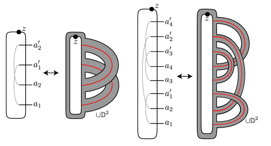
Figure 1.1. Pointed matched circles and surfaces. Left: a pointed matched circle specifying a once-punctured torus. Right: a pointed matched circle specifying a once-punctured genus $2$ surface. In both cases, the involution $M$ exchanges $a_{i}$ and $a^{\prime}_{i}$.

A pointed matched circle specifies a surface. There are a few essentially equivalent constructions; here is one:

Construction 1.2.

Fix a pointed matched circle $\mathcal{Z}=(Z,{\mathbf{a}},M,z)$. Build an oriented surface-with-boundary $F^{\circ}(\mathcal{Z})$ as follows. Start with $[0,1]\times Z$. Attach a strip ($2$-dimensional $1$-handle) to each pair of matched points in ${\mathbf{a}}\times\{0\}$. The result has boundary $(Z\times\{1\})\amalg Z^{\prime}$. Fill in $Z^{\prime}$ with a copy of $\mathbb{D}^{2}$. The result is $F^{\circ}(\mathcal{Z})$. Again, see Figure 1.1.

As a slight variant, we could fill in the boundary of $F^{\circ}(\mathcal{Z})$ with a disk. This gives a surface $F(\mathcal{Z})$ with a distinguished disk in it—the disk $F(\mathcal{Z})\setminus F^{\circ}(\mathcal{Z})$—and a distinguished basepoint on the boundary of this disk. That is, $F(\mathcal{Z})$ is a strongly based surface. (Papers in the subject sometimes treat a pointed matched circle as specifying a surface with boundary, and sometimes as specifying a closed, strongly based surface; it makes no essential difference.)

Remark 1.3.

Pointed matched circles are a special case of Zarev’s arc diagrams; any orientable surface with non-empty boundary can be represented by an arc diagram, and there is an associated algebra similar to the one we will describe in Section 1.4.3. Arc diagrams are, in turn, closely related to fat graphs and chord diagrams.

1.2. Bordered Heegaard diagrams for $3$-manifolds

We start with $3$-manifolds with one boundary component:

Definition 1.4.

A bordered $3$-manifold consists of a compact, oriented $3$-manifold-with-boundary $Y$ and a homeomorphism $\phi\nobreak\mskip 2.0mu\mathpunct{}\nonscript\mkern-3.0mu{:}\penalty 300\mskip 6.0mu plus 1.0muF(\mathcal{Z})\to\partial Y$ for some pointed matched circle $\mathcal{Z}$.

Call two bordered $3$-manifolds $(Y_{1},\phi_{1}\nobreak\mskip 2.0mu\mathpunct{}\nonscript\mkern-3.0mu{:}\penalty 300\mskip 6.0mu plus 1.0muF(\mathcal{Z})\to\partial Y_{1})$ and $(Y_{2},\phi_{2}\nobreak\mskip 2.0mu\mathpunct{}\nonscript\mkern-3.0mu{:}\penalty 300\mskip 6.0mu plus 1.0muF(\mathcal{Z})\to\partial Y_{2})$ equivalent if there is a homeomorphism $\psi\nobreak\mskip 2.0mu\mathpunct{}\nonscript\mkern-3.0mu{:}\penalty 300\mskip 6.0mu plus 1.0muY_{1}\to Y_{2}$ so that $\phi_{2}=\psi\circ\phi_{1}$, i.e.,

commutes.

We often drop the parametrization $\phi$ from the notation, writing $Y$ to denote a bordered $3$-manifold, i.e., $Y=(Y,\phi)$.

We can represent bordered $3$-manifolds combinatorially, as follows:

Definition 1.5.

Let $\mathcal{Z}$ be a pointed matched circle representing a surface of genus $k$. A bordered Heegaard diagram with boundary $\mathcal{Z}$ is a tuple

$$\mathcal{H}=(\Sigma_{g},\overbrace{\overbrace{\alpha_{1}^{a},\dots,\alpha_{2k}^{a}}^{{\boldsymbol{\alpha}}^{a}},\overbrace{\alpha_{1}^{c},\dots,\alpha_{g-k}^{c}}^{{\boldsymbol{\alpha}}^{c}}}^{{\boldsymbol{\alpha}}},\overbrace{\beta_{1},\dots,\beta_{g}}^{{\boldsymbol{\beta}}},z)$$

where

• $\Sigma_{g}$ is a compact, oriented surface of genus $g$ with one boundary component.

• ${\boldsymbol{\beta}}$ is a $g$-tuple of pairwise disjoint circles in the interior of ${\Sigma}$.

• ${\boldsymbol{\alpha}}^{c}$ is a $(g-k)$-tuple of pairwise disjoint circles in the interior of ${\Sigma}$.

• ${\boldsymbol{\alpha}}^{a}$ is a $(2k)$-tuple of pairwise disjoint arcs in $\Sigma$ with boundary in $\partial\Sigma$.

• $z$ is a basepoint in $\partial\Sigma\setminus{\boldsymbol{\alpha}}^{a}$.

• ${\boldsymbol{\alpha}}^{a}\cap{\boldsymbol{\alpha}}^{c}=\emptyset$.

• $\Sigma\setminus({\boldsymbol{\alpha}}^{c}\cup{\boldsymbol{\alpha}}^{a})$ and $\Sigma\setminus{\boldsymbol{\beta}}$ are both connected.

• $\mathcal{Z}=(\partial\Sigma,{\boldsymbol{\alpha}}^{a}\cap\partial\Sigma,M,z)$. Here, $M$ matches (exchanges) the two endpoints of each $\alpha_{i}^{a}$.

Especially when we are considering holomorphic curves, we will abuse notation and also use $\Sigma$ to denote $\Sigma\setminus\partial\Sigma$; and similarly for the $\alpha$-arcs.

Construction 1.6.

Let $\mathcal{H}=(\Sigma,{\boldsymbol{\alpha}},{\boldsymbol{\beta}},z)$ be a bordered Heegaard diagram with boundary $\mathcal{Z}$. There is a corresponding bordered $3$-manifold $Y(\mathcal{H})$ constructed as follows.

1. Thicken ${\Sigma}$ to ${\Sigma}\times[0,1]$.

2. Attach three-dimensional two-handles along the $\alpha$-circles in ${\Sigma}\times\{0\}$.

3. Attach three-dimensional two-handles along the $\beta$-circles in ${\Sigma}\times\{1\}$.

Figure 1.2. A bordered Heegaard diagram and the associated $3$-manifold. The picture on the left is a Heegaard diagram for the bordered solid torus shown on the right. (The labels $A$ indicate a handle between the corresponding circles.) The shaded part of the boundary is $F^{\circ}(\mathcal{Z})$. This figure is adapted from [LOT10a, Figure LABEL:LOT2:fig:PBHD-3-mfld].

A parameterization of the boundary is specified as follows. Consider the graph

$$\left({{\boldsymbol{\alpha}}}^{a}\cup\left(\partial{\Sigma}\setminus\operatorname{nbd}(z)\right)\right)\times\{0\}\subset{\Sigma}\times\{0\},$$

thought of as a subset of $\partial Y$. The closure $F^{\circ}$ of a neighborhood of this graph is naturally identified with $F^{\circ}(\mathcal{Z})$. The complement of $F^{\circ}$ in $\partial Y$ is a disk, and is identified with $F(\mathcal{Z})\setminus F^{\circ}(\mathcal{Z})$. See Figure 1.2.

The orientations in Construction 1.6 are confusing; see [LOT10a, Construction LABEL:LOT2:construct:bordered-HD-to-bordered-Y-one-bdy] for a discussion of this point.

Example 1.7.

Figure 1.2 shows a Heegaard diagram for a solid torus. This is one of many Heegaard diagrams for bordered solid tori; see Section 2.4 for more Heegaard diagrams for solid tori.

Example 1.8.

Figure 5.6 (page 5.6) shows a Heegaard diagram for a genus $2$ handlebody. Again, this is one among many.

Example 1.9.

Fix an oriented surface $\Sigma$, equipped with a $g$-tuple of pairwise disjoint, homologically independent curves ${\boldsymbol{\beta}}$ and a $(g-1)$-tuple of pairwise disjoint, homologically independent curves ${\boldsymbol{\alpha}}^{c}=\{\alpha_{1}^{c},\dots,\alpha_{1}^{g-1}\}$. Then $(\Sigma,{\boldsymbol{\alpha}}^{c},{\boldsymbol{\beta}})$ is a Heegaard diagram for a three-manifold with torus boundary, and indeed any such three-manifold $Y$ can be described by a Heegaard diagram of this type. To turn such a diagram into a bordered Heegaard diagram, we proceed as follows. Fix an additional pair of circles $\gamma_{1}$ and $\gamma_{2}$ in $\Sigma$ so that:

• $\gamma_{1}$ and $\gamma_{2}$ are disjoint from $\alpha_{1}^{c},\dots,\alpha_{g-1}^{c}$,

• $\gamma_{1}$ and $\gamma_{2}$ intersect, transversally, in a single point $p$ and

• both of the homology classes $[\gamma_{1}]$ and $[\gamma_{2}]$ are homologically independent from $[\alpha_{1}^{c}],\dots,[\alpha_{g-1}^{c}]$.

Let $D$ be a disk around $p$ which is disjoint from all the above curves, except for $\gamma_{1}$ and $\gamma_{2}$, each of which it meets in a single arc. Then, the complement of $D$ specifies a bordered Heegaard diagram for $Y$, for some parametrization of $\partial Y$. A bordered Heegaard diagram for the trefoil complement is illustrated in Figure 1.3.

\begin{overpic}[tics=10,scale={.85714}]{Trefoil_bord_HD} \put(94.0,2.0){{\color[rgb]{0,0,1}$\beta_{2}$}} \end{overpic}

Figure 1.3. A bordered Heegaard diagram for the trefoil complement. Left: a Heegaard diagram for the complement of the trefoil. The circles labeled $A$ (respectively $B$) denote a handle attached to the plane. Right: a bordered Heegaard diagram, obtained by adding the curves $\gamma_{1}$ and $\gamma_{2}$ and deleting a disk. It may be instructive to compare this diagram with Figure 4.1

(This example is drawn from [LOT08, Section LABEL:LOT1:sec:Bestiary]; see also the discussion around [LOT08, Figure LABEL:LOT1:fig:Twisting].)

We also consider $3$-dimensional cobordisms:

Definition 1.10.

Fix pointed matched circles

$$\mathcal{Z}_{L} =(Z_{L},{\mathbf{a}}_{L},M_{L},z_{L})$$

$$\mathcal{Z}_{R} =(Z_{R},{\mathbf{a}}_{R},M_{R},z_{R}).$$

An arced cobordism from $\mathcal{Z}_{L}$ to $\mathcal{Z}_{R}$ consists of:

• A compact, oriented $3$-manifold-with-boundary $Y$,

• an injection $\phi\nobreak\mskip 2.0mu\mathpunct{}\nonscript\mkern-3.0mu{:}\penalty 300\mskip 6.0mu plus 1.0mu(-F^{\circ}(\mathcal{Z}_{L}))\amalg F^{\circ}(\mathcal{Z}_{R})\to\partial Y$ (where $-$ denotes orientation reversal) and

• a path $\gamma$ in $\partial Y\setminus\mathrm{Im}(\phi)$

such that $Y\setminus(\mathrm{Im}(\phi)\cup\operatorname{nbd}(\gamma))$ is a disk.

There is a natural notion of equivalence for arced cobordisms, similar to the notion of equivalence for bordered $3$-manifolds; we leave it as an exercise.

As for bordered $3$-manifolds, we will typically denote all of the data of an arced cobordism simply by $Y$. Also as with bordered $3$-manifolds, there are several other essentially equivalent ways to formulate the notion of an arced cobordism; see for instance [LOT10a, Section LABEL:LOT2:sec:Diagrams] and [LOT11a, Section LABEL:HomPair:sec:ab].

Again, a combinatorial representation of arced cobordisms will be important to us:

Definition 1.11.

An arced Heegaard diagram is a tuple

$$\mathcal{H}=(\Sigma_{g},\overbrace{\overbrace{\alpha_{1}^{a,L},\dots,\alpha_{2k_{L}}^{a,L}}^{{\boldsymbol{\alpha}}^{a,L}},\overbrace{\alpha_{1}^{a,R},\dots,\alpha_{2k_{R}}^{a,R}}^{{\boldsymbol{\alpha}}^{a,R}},\overbrace{\alpha_{1}^{c},\dots,\alpha_{g-k_{L}-k_{R}}^{c}}^{{\boldsymbol{\alpha}}^{c}}}^{{\boldsymbol{\alpha}}},\overbrace{\beta_{1},\dots,\beta_{g}}^{{\boldsymbol{\beta}}},\mathbf{z})$$

where

• ${\Sigma}_{g}$ is a compact, oriented surface of genus $g$ with two boundary components, $\partial_{L}\Sigma$ and $\partial_{R}\Sigma$;

• ${\boldsymbol{\beta}}$ is a $g$-tuple of pairwise disjoint curves in the interior of ${\Sigma}$;

• ${\boldsymbol{\alpha}}^{a,L}$ is a collection of pairwise-disjoint embedded arcs with boundary on $\partial_{L}{\Sigma}$;

• ${\boldsymbol{\alpha}}^{a,R}$ is a collection of pairwise-disjoint embedded arcs with boundary on $\partial_{R}{\Sigma}$;

• ${\boldsymbol{\alpha}}^{c}$ is a collection of pairwise-disjoint circles in the interior of ${\Sigma}$; and

• $\mathbf{z}$ is a path in ${\Sigma}\setminus({\boldsymbol{\alpha}}^{a,L}\cup{\boldsymbol{\alpha}}^{a,R}\cup{\boldsymbol{\alpha}}^{c}\cup{\boldsymbol{\beta}})$ between $\partial_{L}{\Sigma}$ and $\partial_{R}{\Sigma}$.

These are required to satisfy:

• ${\boldsymbol{\alpha}}^{a,L}$, ${\boldsymbol{\alpha}}^{a,R}$ and ${\boldsymbol{\alpha}}$ are all disjoint,

• ${\Sigma}\setminus{{\boldsymbol{\alpha}}}$ and ${\Sigma}\setminus{\boldsymbol{\beta}}$ are connected and

• ${{\boldsymbol{\alpha}}}$ intersects ${\boldsymbol{\beta}}$ transversely.

(Compare [LOT10a, Definition LABEL:LOT2:def:ArcedBordered].)

Observe that each boundary component of an arced Heegaard diagram is a pointed matched circle.

Figure 1.4. Constructing a bordered 3-manifold with two boundary components from an arced bordered Heegaard diagram. The Heegaard diagram on the left represents an elementary cobordism from the genus two surface to the genus one surface. On the right is a (somewhat schematic) depiction of the resulting $3$-manifold. The inside part of the boundary, which corresponds to $\Sigma\times\{1\}$, is a cylinder, since the $\beta$-circles caused the handles to be filled in. The outside part of the boundary, corresponding to $\Sigma\times\{0\}$, is a surface of genus $3$ with two boundary components. The region $F^{\circ}_{L}$ (respectively $F^{\circ}_{R}$) is darkly (respectively lightly) shaded.

Construction 1.12.

Fix an arced Heegaard diagram $\mathcal{H}=(\Sigma_{g},{\boldsymbol{\alpha}}^{a,L},{\boldsymbol{\alpha}}^{a,R},{\boldsymbol{\alpha}}^{c},{\boldsymbol{\beta}},\mathbf{z})$ with boundary $\mathcal{Z}_{L}\amalg\mathcal{Z}_{R}$. Build a $3$-manifold-with-boundary $Y$ as follows:

1. Thicken ${\Sigma}$ to ${\Sigma}\times[0,1]$.

2. Attach three-dimensional two-handles along the $\alpha$-circles in ${\Sigma}\times\{0\}$.

3. Attach three-dimensional two-handles along the $\beta$-circles in ${\Sigma}\times\{1\}$.

Consider the graphs

$$\Gamma_{L} =\left({{\boldsymbol{\alpha}}}^{a,L}\cup\left(\partial_{L}{\Sigma}\setminus\operatorname{nbd}(\mathbf{z})\right)\right)\times\{0\}\subset{\Sigma}\times\{0\}$$

$$\Gamma_{R} =\left({{\boldsymbol{\alpha}}}^{a,R}\cup\left(\partial_{R}{\Sigma}\setminus\operatorname{nbd}(\mathbf{z})\right)\right)\times\{0\}\subset{\Sigma}\times\{0\}$$

thought of as subsets of $\partial Y$. The closure $F^{\circ}_{L}$ (respectively $F^{\circ}_{R}$) of a neighborhood of $\Gamma_{L}$ (respectively $\Gamma_{R}$) is naturally identified with $F^{\circ}(\mathcal{Z}_{L})$ (respectively $F^{\circ}(\mathcal{Z}_{R})$). Let $\phi$ denote this identification $F^{\circ}(\mathcal{Z}_{L})\amalg F^{\circ}(\mathcal{Z}_{R})\to F^{\circ}_{L}\amalg F^{\circ}_{R}$. The arc $\gamma_{\mathbf{z}}=\mathbf{z}\times\{0\}$ connects $F^{\circ}_{L}$ and $F^{\circ}_{R}$, and $\partial Y\setminus(F^{\circ}_{L}\cup F^{\circ}_{R}\cup\operatorname{nbd}(\gamma_{\mathbf{z}}))$ is a disk. The data $(Y,\phi,\gamma_{\mathbf{z}})$ is an arced cobordism; we call this cobordism the arced cobordism associated to $\mathcal{H}$ and denote it by $Y(\mathcal{H})$. See Figure 1.4.

Example 1.13.

Let $\psi\nobreak\mskip 2.0mu\mathpunct{}\nonscript\mkern-3.0mu{:}\penalty 300\mskip 6.0mu plus 1.0muF(\mathcal{Z}_{L})\to F(\mathcal{Z}_{R})$ be a homeomorphism taking the preferred disk to the preferred disk and the basepoint to the basepoint; that is, $\psi$ is a strongly based homeomorphism. The mapping cylinder of $\psi$, denoted $M_{\psi}$, is the arced cobordism from $\mathcal{Z}_{L}$ to $\mathcal{Z}_{R}$ given as follows. The underlying $3$-manifold is $[0,1]\times F^{\circ}(\mathcal{Z}_{R})$. The map $\phi\nobreak\mskip 2.0mu\mathpunct{}\nonscript\mkern-3.0mu{:}\penalty 300\mskip 6.0mu plus 1.0mu-F^{\circ}(\mathcal{Z}_{L})\amalg F^{\circ}(\mathcal{Z}_{R})\to\partial M_{\psi}$ is given by the identity map $\mathbb{I}\nobreak\mskip 2.0mu\mathpunct{}\nonscript\mkern-3.0mu{:}\penalty 300\mskip 6.0mu plus 1.0muF^{\circ}(\mathcal{Z}_{R})\to\{1\}\times F^{\circ}(\mathcal{Z}_{R})$ and the map $\psi\nobreak\mskip 2.0mu\mathpunct{}\nonscript\mkern-3.0mu{:}\penalty 300\mskip 6.0mu plus 1.0muF^{\circ}(\mathcal{Z}_{L})\to\{0\}\times F^{\circ}(\mathcal{Z}_{R})$. The arc $\gamma$ is $[0,1]\times\{z\}$.

Some examples of Heegaard diagrams for mapping cylinders are shown in Figure 2.3.

Gluing the mapping cylinder for $\psi$ to a bordered $3$-manifold $(Y,\phi)$ in the sense of Exercise 1.2 gives $(Y,\phi\circ\psi)$.

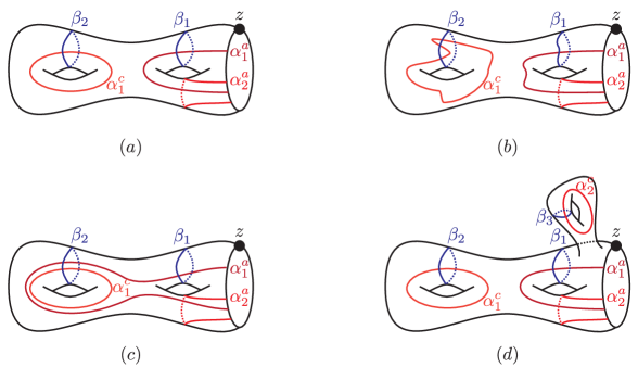
Figure 1.5. Heegaard moves. (a) A genus $2$ bordered Heegaard diagram for a solid torus. (b) The result of applying some isotopies to the $\alpha$- and $\beta$-curves. (c) The result of a handleslide of $\alpha_{1}^{a}$ over $\alpha_{1}^{c}$. (d) The result of a stabilization.

As in the closed case, the key properties of bordered Heegaard diagrams are that every bordered $3$-manifold can be represented by a bordered Heegaard diagram, and any two such diagrams can be related by certain elementary moves:

Theorem 1.14.

Let $(Y,\phi\nobreak\mskip 2.0mu\mathpunct{}\nonscript\mkern-3.0mu{:}\penalty 300\mskip 6.0mu plus 1.0muF(\mathcal{Z})\to\partial Y)$ be a bordered $3$-manifold. Then $Y$ is represented by some bordered Heegaard diagram $\mathcal{H}$. Similarly, let $(Y,\phi\nobreak\mskip 2.0mu\mathpunct{}\nonscript\mkern-3.0mu{:}\penalty 300\mskip 6.0mu plus 1.0muF^{\circ}(\mathcal{Z}_{L})\amalg F^{\circ}(\mathcal{Z}_{R})\to\partial Y,\gamma)$ be an arced cobordisms. Then $Y$ is represented by some arced Heegaard diagram $\mathcal{H}$.

The case of bordered Heegaard diagrams is [LOT08, Lemma LABEL:LOT1:lem:3mfld-heegaard] while the arced Heegaard diagram case is [LOT10a, Proposition LABEL:LOT2:prop:diagrams-exist].

Theorem 1.15.

Suppose that $\mathcal{H}$ and $\mathcal{H}^{\prime}$ are bordered Heegaard diagrams representing equivalent bordered $3$-manifolds $Y(\mathcal{H})\cong Y(\mathcal{H}^{\prime})$. Then $\mathcal{H}$ and $\mathcal{H}^{\prime}$ can be made diffeomorphic by a sequence of the following moves:

• Isotopies of the $\alpha$- and/or $\beta$-curves.

• Handleslides or $\alpha$-circles over $\alpha$-circles, $\alpha$-arcs over $\alpha$-circles, and $\beta$-circles over $\beta$-circles.

• Stabilizations and destabilizations of the diagram, i.e., taking connected sums with the standard Heegaard diagram for $S^{3}$.

(See Figure 1.5.)

An exactly analogous statement holds for arced Heegaard diagrams and arced cobordisms.

The case of bordered Heegaard diagrams is [LOT08, Proposition LABEL:LOT1:prop:heegaard-moves] while the arced Heegaard diagram case is [LOT10a, Proposition LABEL:LOT2:prop:heegaard-moves].

1.3. The structure of bordered Floer homology

1.3.1. The connected boundary case

For simplicity, we begin with the connected boundary case. Bordered Floer homology assigns:

Pointed matched circle $\mathcal{Z}$	dg algebra $\mathcal{A}(\mathcal{Z})$
Bordered $3$-manifold $(Y,\phi\nobreak\mskip 2.0mu\mathpunct{}\nonscript\mkern-3.0mu{:}\penalty 300\mskip 6.0mu plus 1.0muF(\mathcal{Z})\to\partial Y)$	Right $A_{\infty}$ $\mathcal{A}(\mathcal{Z})$-module $\widehat{\mathit{CFA}}(Y)$
	Left dg $\mathcal{A}(-\mathcal{Z})$-module $\widehat{\mathit{CFD}}(Y)$.

Actually, the modules $\widehat{\mathit{CFA}}(Y)$ and $\widehat{\mathit{CFD}}(Y)$ depend on a choice of bordered Heegaard diagram $\mathcal{H}$ for $Y$, as well as another auxiliary choice—an almost-complex structure. However:

Theorem 1.16.

[LOT08, Theorems LABEL:LOT1:intro:D-invariance and LABEL:LOT1:intro:A-invariance] The quasi-isomorphism types of the modules $\widehat{\mathit{CFA}}(Y)$ and $\widehat{\mathit{CFD}}(Y)$ depend only on the equivalence class of bordered $3$-manifold $Y$.

The utility of $\widehat{\mathit{CFA}}$ and $\widehat{\mathit{CFD}}$ comes from the fact that they can be used to reconstruct the Heegaard Floer homology groups of closed three-manifolds $\widehat{\mathit{HF}}(Y)$, via what we call a pairing theorem. Recall that $\widehat{\mathit{HF}}(Y)$ is the homology of a chain complex $\widehat{\mathit{CF}}(Y)$.

Theorem 1.17.

[LOT08, Theorem LABEL:LOT1:thm:TensorPairing] Suppose that $(Y_{1},\phi_{1}\nobreak\mskip 2.0mu\mathpunct{}\nonscript\mkern-3.0mu{:}\penalty 300\mskip 6.0mu plus 1.0muF(\mathcal{Z})\to\partial Y)$ and $(Y_{2},\phi_{2}\nobreak\mskip 2.0mu\mathpunct{}\nonscript\mkern-3.0mu{:}\penalty 300\mskip 6.0mu plus 1.0mu{-F(\mathcal{Z})}\to\partial Y)$ are bordered $3$-manifolds with boundaries parameterized by $\mathcal{Z}$ and $-\mathcal{Z}$, respectively. Write $Y_{1}\cup_{\partial}Y_{2}$ to mean $\bigl{(}Y_{1}\amalg Y_{2})/(\phi_{1}(x)\sim\phi_{2}(x))$. Then

$$\widehat{\mathit{CF}}(Y)\simeq\widehat{\mathit{CFA}}(Y_{1})\mathop{\widetilde{\otimes}}\nolimits_{\mathcal{A}(F)}\widehat{\mathit{CFD}}(Y_{2}).$$

Here, $\mathop{\widetilde{\otimes}}\nolimits$ denotes the appropriate notion of tensor product given that $\widehat{\mathit{CFA}}$ may be an $A_{\infty}$-module. In the case that $\widehat{\mathit{CFA}}$ is an ordinary module, this reduces to the derived tensor product—which is good, since $\widehat{\mathit{CFA}}$ is only well-defined up to quasi-isomorphism. But this distinction is not so important: the module $\widehat{\mathit{CFD}}$ is projective, so the derived and ordinary tensor products agree.

The modules $\widehat{\mathit{CFA}}(Y)$ and $\widehat{\mathit{CFD}}(Y)$ are defined using holomorphic curves (though for certain kinds of diagrams the techniques of [SW10] can be used to compute them combinatorially). By contrast, the algebras $\mathcal{A}(\mathcal{Z})$ are defined combinatorially. A few further properties of the algebras:

• Each $\mathcal{A}(\mathcal{Z})$ is a finite-dimensional algebra over ${\mathbb{F}_{2}}$.

• The algebra $\mathcal{A}(\mathcal{Z})$ decomposes as a direct sum of subalgebras

  $$\mathcal{A}(\mathcal{Z})=\bigoplus_{i=-k}^{k}\mathcal{A}(\mathcal{Z},i).$$

  Here, $k$ is the genus of $F(\mathcal{Z})$. The action of $\mathcal{A}(\mathcal{Z},i)$ on $\widehat{\mathit{CFA}}(Y)$ and $\widehat{\mathit{CFD}}(Y)$ is trivial for $i\neq 0$, but the other summands come up for the cobordism invariants below.

• The algebra $\mathcal{A}(\mathcal{Z},-k)$ is isomorphic to ${\mathbb{F}_{2}}$ (with trivial differential). In particular, if $\mathcal{Z}$ is the (unique) pointed matched circle for $S^{2}$ then $\mathcal{A}(\mathcal{Z})={\mathbb{F}_{2}}$. The algebra $\mathcal{A}(\mathcal{Z},k)$ is quasi-isomorphic to ${\mathbb{F}_{2}}$.

• If $\mathcal{Z}$ is the unique pointed matched circle for the torus then $\mathcal{A}(\mathcal{Z},0)$ has no differential; in terms of generators and relations, $\mathcal{A}(\mathcal{Z},0)$ is given by

  (1.18) $$\lx@xy@svg{\hbox{\raise 0.0pt\hbox{\kern 8.6697pt\hbox{\ignorespaces\ignorespaces\ignorespaces\hbox{\vtop{\kern 0.0pt\offinterlineskip\halign{\entry@#!@&&\entry@@#!@\cr&\crcr}}}\ignorespaces{\hbox{\kern-8.6697pt\raise 0.0pt\hbox{\hbox{\kern 0.0pt\raise 0.0pt\hbox{\hbox{\kern 3.0pt\raise 0.0pt\hbox{$\textstyle{\iota_{0}\bullet\ignorespaces\ignorespaces\ignorespaces\ignorespaces\ignorespaces\ignorespaces\ignorespaces\ignorespaces\ignorespaces\ignorespaces}$}}}}}}}\ignorespaces\ignorespaces\ignorespaces\ignorespaces\ignorespaces{}{}{}{{}{}{}{}{}{}{}{}{}{}{}{}{}{}{}}{}\ignorespaces\hbox{\hbox{\kern 0.0pt\raise 0.0pt\hbox{{}{}{{}}{{}{}{}}{}}}}\ignorespaces{}\ignorespaces{}{}{}{{}{}}\ignorespaces\ignorespaces{\hbox{\kern 15.41571pt\raise 17.1875pt\hbox{{}\hbox{\kern 0.0pt\raise 0.0pt\hbox{\hbox{\kern 3.0pt\hbox{\hbox{\kern 0.0pt\raise-0.8264pt\hbox{$\scriptstyle{\rho_{1}}$}}}\kern 3.0pt}}}}}}\ignorespaces{}{}{}{{}{}{}{}{}{}{}{}{}{}{}{}{}{}{}{}{}{}{}}{\hbox{\kern 34.3045pt\raise 7.44342pt\hbox{\hbox{\kern 0.0pt\raise 0.0pt\hbox{\lx@xy@tip{1}\lx@xy@tip{-1}}}}}}\ignorespaces\hbox{\hbox{\kern 0.0pt\raise 0.0pt\hbox{{}{}{}{{}}{{}{}{}\lx@xy@spline@}{}}}}\ignorespaces{}\ignorespaces\hbox{\hbox{\kern 0.0pt\raise 0.0pt\hbox{{}{}{{}}{{}{}{}}{}}}}\ignorespaces{}\ignorespaces\ignorespaces\ignorespaces\ignorespaces\ignorespaces{}{}{}{{}{}{}{}{}{}{}{}{}{}{}{}{}{}{}{}{}}{}\ignorespaces\hbox{\hbox{\kern 0.0pt\raise 0.0pt\hbox{{}{}{{}}{{}{}{}}{}}}}\ignorespaces{}\ignorespaces{}{}{}{{}{}}\ignorespaces\ignorespaces{\hbox{\kern 15.41571pt\raise-17.18748pt\hbox{{}\hbox{\kern 0.0pt\raise 0.0pt\hbox{\hbox{\kern 3.0pt\hbox{\hbox{\kern 0.0pt\raise-0.8264pt\hbox{$\scriptstyle{\rho_{3}}$}}}\kern 3.0pt}}}}}}\ignorespaces{}{}{}{{}{}{}{}{}{}{}{}{}{}{}{}{}{}{}{}{}}{\hbox{\kern 37.66241pt\raise-4.8034pt\hbox{\hbox{\kern 0.0pt\raise 0.0pt\hbox{\lx@xy@tip{1}\lx@xy@tip{-1}}}}}}\ignorespaces\hbox{\hbox{\kern 0.0pt\raise 0.0pt\hbox{{}{}{}{{}}{{}{}{}\lx@xy@spline@}{}}}}\ignorespaces{}\ignorespaces\hbox{\hbox{\kern 0.0pt\raise 0.0pt\hbox{{}{}{{}}{{}{}{}}{}}}}\ignorespaces{}{\hbox{\kern 32.6697pt\raise 0.0pt\hbox{\hbox{\kern 0.0pt\raise 0.0pt\hbox{\hbox{\kern 3.0pt\raise 0.0pt\hbox{$\textstyle{\bullet\iota_{1}\ignorespaces\ignorespaces\ignorespaces\ignorespaces}$}}}}}}}\ignorespaces\ignorespaces\ignorespaces\ignorespaces{}{\hbox{\lx@xy@droprule}}\ignorespaces\ignorespaces\ignorespaces{\hbox{\kern 15.4157pt\raise 5.1875pt\hbox{{}\hbox{\kern 0.0pt\raise 0.0pt\hbox{\hbox{\kern 3.0pt\hbox{\hbox{\kern 0.0pt\raise-0.8264pt\hbox{$\scriptstyle{\rho_{2}}$}}}\kern 3.0pt}}}}}}\ignorespaces{\hbox{\kern 8.6697pt\raise 0.0pt\hbox{\hbox{\kern 0.0pt\raise 0.0pt\hbox{\lx@xy@tip{1}\lx@xy@tip{-1}}}}}}{\hbox{\lx@xy@droprule}}{\hbox{\lx@xy@droprule}}\ignorespaces}}}}\ignorespaces/(\rho_{2}\rho_{1}=\rho_{3}\rho_{2}=0). \textstyle{\iota_{0}\bullet\ignorespaces\ignorespaces\ignorespaces\ignorespaces\ignorespaces\ignorespaces\ignorespaces\ignorespaces\ignorespaces\ignorespaces} \scriptstyle{\rho_{1}} \scriptstyle{\rho_{3}} \textstyle{\bullet\iota_{1}\ignorespaces\ignorespaces\ignorespaces\ignorespaces} \scriptstyle{\rho_{2}} \textstyle{\iota_{0}\bullet\ignorespaces\ignorespaces\ignorespaces\ignorespaces\ignorespaces\ignorespaces\ignorespaces\ignorespaces\ignorespaces\ignorespaces} \scriptstyle{\rho_{1}} \scriptstyle{\rho_{3}} \textstyle{\bullet\iota_{1}\ignorespaces\ignorespaces\ignorespaces\ignorespaces} \scriptstyle{\rho_{2}}$$

  This algebra is $8$-dimensional over ${\mathbb{F}_{2}}$. It will appear frequently, so we name the rest of the elements in its standard basis: let $\rho_{12}=\rho_{1}\rho_{2}$, $\rho_{23}=\rho_{2}\rho_{3}$ and $\rho_{123}=\rho_{1}\rho_{2}\rho_{3}$.

  (Our notation for path algebras might be somewhat non-standard. The vertices $\iota_{0}$ and $\iota_{1}$ are, of course, idempotents. The arrow $\rho_{1}$ indicates that $\iota_{0}\rho_{1}\iota_{1}=\rho_{1}$.)

1.3.2. Invariants of arced cobordisms

To get a useful theory, we need to generalize to three-manifolds with two boundary components. In fact, the invariants which come up in this two-boundary-component case are associated to three-manifolds equipped with some extra structure: the arced cobordisms of Definition 1.10.

Suppose $Y$ is an arced cobordism from $\mathcal{Z}_{1}$ to $\mathcal{Z}_{2}$. Then there are several kinds of bimodules we can associate to $Y$: we can treat each boundary component of $Y$ in either a “type $D$” way or a “type $A$” way. (What this means will be clearer after Lectures 2 and 3.) This gives invariants $\widehat{\mathit{CFDD}}(Y)$ (both boundaries viewed in a type $D$ way), $\widehat{\mathit{CFDA}}(Y)$ (one boundary, say $\mathcal{Z}_{1}$, viewed in a type $D$ way and the other in a type $A$ way), and $\widehat{\mathit{CFAA}}(Y)$ (both boundaries viewed in a type $A$ way). The bimodule $\widehat{\mathit{CFDD}}(Y)$ is an ordinary—indeed, bi-projective—dg bimodule; both of $\widehat{\mathit{CFDA}}(Y)$ and $\widehat{\mathit{CFAA}}(Y)$ are typically $A_{\infty}$-bimodules.

As with the modules associated to bordered $3$-manifolds, the bimodules $\widehat{\mathit{CFDD}}(Y)$, $\widehat{\mathit{CFDA}}(Y)$ and $\widehat{\mathit{CFAA}}(Y)$ depend on the choices of Heegaard diagrams and almost-complex structures. Again, up to quasi-isomorphism they are invariants:

Theorem 1.19.

[LOT10a, Theorem LABEL:LOT2:thm:InvarianceOfBimodules] The quasi-isomorphism types of the bimodules $\widehat{\mathit{CFDD}}(Y)$, $\widehat{\mathit{CFDA}}(Y)$ and $\widehat{\mathit{CFAA}}(Y)$ depend only on the equivalence class of arced cobordism $Y$.

By convention, we view $\widehat{\mathit{CFDD}}(Y)$ as having commuting left actions by $\mathcal{A}(-\mathcal{Z}_{1})$ and $\mathcal{A}(-\mathcal{Z}_{2})$; $\widehat{\mathit{CFDA}}(Y)$ as having a left action by $\mathcal{A}(-\mathcal{Z}_{1})$ and a right action by $\mathcal{A}(\mathcal{Z}_{2})$; and $\widehat{\mathit{CFAA}}(Y)$ as having right actions by $\mathcal{A}(\mathcal{Z}_{1})$ and $\mathcal{A}(\mathcal{Z}_{2})$. However, $\mathcal{A}(-\mathcal{Z})$ is the opposite algebra to $\mathcal{A}(\mathcal{Z})$ (Exercise 1.13) so we can move actions from one side to the other at the cost of introducing / deleting minus signs. In the literature, we often find it convenient to decorate the invariants with the algebras they are over, writing

$${}^{\mathcal{A}(-\mathcal{Z}_{1}),\mathcal{A}(-\mathcal{Z}_{2})}\mskip-1.80002mu\widehat{\mathit{CFDD}}(Y)\qquad\qquad{}^{\mathcal{A}(-\mathcal{Z}_{1})}\mskip-1.80002mu\widehat{\mathit{CFDA}}(Y)_{\mathcal{A}(\mathcal{Z}_{2})}\qquad\qquad\widehat{\mathit{CFAA}}(Y)_{\mathcal{A}(\mathcal{Z}_{1}),\mathcal{A}(\mathcal{Z}_{1})}.$$

The superscripts indicate that the module structure is projective, and subscripts indicate the module structure may be $A_{\infty}$. This notation leads to a kind of Einstein summation behavior for tensor products in the pairing theorems:

Theorem 1.20.

[LOT10a, Theorem LABEL:LOT2:thm:GenReparameterization] Let $Y_{1}$ be a bordered $3$-manifold with boundary $\mathcal{Z}_{1}$ and $Y_{2}$ be an arced cobordism from $\mathcal{Z}_{1}$ to $\mathcal{Z}_{2}$. Let $Y_{1}\cup_{F(\mathcal{Z})}Y_{2}$ be the bordered $3$-manifold obtained by gluing $Y_{1}$ to $Y_{2}$ (Exercise 1.2). Then there are quasi-isomorphisms

$$\widehat{\mathit{CFA}}(Y_{1})\mathop{\widetilde{\otimes}}\nolimits_{\mathcal{A}(\mathcal{Z}_{1})}\widehat{\mathit{CFDA}}(Y_{2}) \simeq\widehat{\mathit{CFA}}(Y_{1}\cup_{F(\mathcal{Z}_{1})}Y_{2})$$

$$\widehat{\mathit{CFAA}}(Y_{2})\mathop{\widetilde{\otimes}}\nolimits_{\mathcal{A}(-\mathcal{Z}_{1})}\widehat{\mathit{CFD}}(Y_{1}) \simeq\widehat{\mathit{CFA}}(Y_{1}\cup_{F(\mathcal{Z}_{1})}Y_{2})$$

$$\widehat{\mathit{CFA}}(Y_{1})\mathop{\widetilde{\otimes}}\nolimits_{\mathcal{A}(\mathcal{Z}_{1})}\widehat{\mathit{CFDD}}(Y_{2}) \simeq\widehat{\mathit{CFD}}(Y_{1}\cup_{F(\mathcal{Z}_{1})}Y_{2})$$

$$\widehat{\mathit{CFDA}}(Y_{2})\mathop{\widetilde{\otimes}}\nolimits_{\mathcal{A}(-\mathcal{Z}_{1})}\widehat{\mathit{CFD}}(Y_{1}) \simeq\widehat{\mathit{CFD}}(Y_{1}\cup_{F(\mathcal{Z}_{1})}Y_{2}).$$

Theorem 1.21.

[LOT10a, Theorem LABEL:LOT2:thm:GenComposition] Let $Y_{1}$ be an arced cobordism from $\mathcal{Z}_{1}$ to $\mathcal{Z}_{2}$ and $Y_{2}$ an arced cobordism from $\mathcal{Z}_{2}$ and $\mathcal{Z}_{3}$. Let $Y_{1}\cup_{F(\mathcal{Z}_{2})}Y_{2}$ be the result of gluing $Y_{1}$ to $Y_{2}$ along $F(\mathcal{Z}_{2})$ (Exercise 1.2). Then there are quasi-isomorphisms of bimodules:

$$\widehat{\mathit{CFDA}}(Y_{1})\mathop{\widetilde{\otimes}}\nolimits_{\mathcal{A}(\mathcal{Z}_{2})}\widehat{\mathit{CFDA}}(Y_{2}) \simeq\widehat{\mathit{CFDA}}(Y_{1}\cup_{F(\mathcal{Z}_{2})}Y_{2})$$

$$\widehat{\mathit{CFAA}}(Y_{1})\mathop{\widetilde{\otimes}}\nolimits_{\mathcal{A}(\mathcal{Z}_{2})}\widehat{\mathit{CFDA}}(Y_{2}) \simeq\widehat{\mathit{CFAA}}(Y_{1}\cup_{F(\mathcal{Z}_{2})}Y_{2})$$

$$\widehat{\mathit{CFDA}}(Y_{1})\mathop{\widetilde{\otimes}}\nolimits_{\mathcal{A}(\mathcal{Z}_{2})}\widehat{\mathit{CFDD}}(Y_{2}) \simeq\widehat{\mathit{CFDD}}(Y_{1}\cup_{F(\mathcal{Z}_{2})}Y_{2})$$

$$\widehat{\mathit{CFAA}}(Y_{1})\mathop{\widetilde{\otimes}}\nolimits_{\mathcal{A}(\mathcal{Z}_{2})}\widehat{\mathit{CFDD}}(Y_{2}) \simeq\widehat{\mathit{CFDA}}(Y_{1}\cup_{F(\mathcal{Z}_{2})}Y_{2})$$

The compact way of stating Theorems 1.20 and 1.21 is that if you tensor type $A$ boundaries with type $D$ boundaries then you get what you expect.

1.3.3. Pairing theorems without $A$ modules

To avoid a long detour into $A_{\infty}$ formalism, in most of these lectures we will avoid $\widehat{\mathit{CFA}}$. (The exception will be the discussion of the pairing theorem in Lecture 3.) So, it will be useful to have versions of the pairing theorems—Theorems 1.17, 1.20 and 1.21—making use only of type $D$ modules. We can accomplish this using certain dualities of bordered Floer invariants:

Theorem 1.22.

[LOT11a, Theorem LABEL:HomPair:thm:or-rev] Let $Y$ be a bordered $3$-manifold with boundary $F(\mathcal{Z})$. Let $-Y$ denote $Y$ with its orientation reversed, which has boundary $F(-\mathcal{Z})$. Then there are quasi-isomorphisms:

(1.23) $$\operatorname{Mor}_{\mathcal{A}(-\mathcal{Z})}(\widehat{\mathit{CFD}}(Y),\mathcal{A}(-\mathcal{Z})) \simeq\widehat{\mathit{CFA}}(-Y)$$

(1.24) $$\operatorname{Mor}_{\mathcal{A}(\mathcal{Z})}(\widehat{\mathit{CFA}}(Y),\mathcal{A}(\mathcal{Z})) \simeq\widehat{\mathit{CFD}}(-Y).$$

In Formula (1.23), $\operatorname{Mor}$ denotes the chain complex of module homomorphisms from $\widehat{\mathit{CFD}}(Y)$ to $\mathcal{A}(-\mathcal{Z})$, with differential given by

$$\partial(f)=f\circ\partial_{\widehat{\mathit{CFD}}(Y)}+d_{\mathcal{A}(-\mathcal{Z})}\circ f.$$

So, for instance, the cycles in the $\operatorname{Mor}$ complex are the dg module homomorphisms, i.e., chain maps which respect the module structure. In Formula (1.24), $\operatorname{Mor}$ denotes the chain complex of $A_{\infty}$-morphisms.

Corollary 1.25.

[LOT11a, Theorem LABEL:HomPair:thm:hom-pair] Suppose that $Y_{1}$ and $Y_{2}$ are bordered $3$-manifolds with boundary $F(\mathcal{Z})$. Then

$$\widehat{\mathit{CF}}(-Y_{1}\cup_{F(\mathcal{Z})}Y_{2}) \simeq\operatorname{Mor}_{\mathcal{A}(-\mathcal{Z})}(\widehat{\mathit{CFD}}(Y_{1}),\widehat{\mathit{CFD}}(Y_{2}))$$

$$\simeq\operatorname{Mor}_{\mathcal{A}(\mathcal{Z})}(\widehat{\mathit{CFA}}(Y_{1}),\widehat{\mathit{CFA}}(Y_{2}))$$

so

$$\widehat{\mathit{HF}}(-Y_{1}\cup_{F(\mathcal{Z})}Y_{2}) \simeq\operatorname{Ext}_{\mathcal{A}(-\mathcal{Z})}(\widehat{\mathit{CFD}}(Y_{1}),\widehat{\mathit{CFD}}(Y_{2}))$$

$$\simeq\operatorname{Ext}_{\mathcal{A}(\mathcal{Z})}(\widehat{\mathit{CFA}}(Y_{1}),\widehat{\mathit{CFA}}(Y_{2})).$$

For bimodules the situation is somewhat more subtle: there are a few natural notions of “dual”, and some versions introduce boundary Dehn twists in the bimodules. The following result will be more than sufficient for these lectures:

Theorem 1.26.

[LOT11a, Corollary LABEL:HomPair:cor:bimod-mod-hom-pair] If $Y_{1}$ is a bordered $3$-manifold with boundary $F(\mathcal{Z}_{1})$ and $Y_{2}$ is an arced cobordism from $-\mathcal{Z}_{1}$ to $-\mathcal{Z}_{2}$ then

(1.27) $$\begin{split}\widehat{\mathit{CFA}}(Y_{1}\cup_{F(\mathcal{Z}_{1})}(-Y_{2}))&\simeq\operatorname{Mor}_{\mathcal{A}(-\mathcal{Z}_{1})}(\widehat{\mathit{CFDD}}(Y_{2}),\widehat{\mathit{CFD}}(Y_{1}))\\ \widehat{\mathit{CFD}}(-Y_{1}\cup_{F(\mathcal{Z}_{1})}Y_{2})&\simeq\operatorname{Mor}_{\mathcal{A}(-\mathcal{Z}_{1})}(\widehat{\mathit{CFD}}(Y_{1}),\widehat{\mathit{CFDD}}(Y_{2})).\end{split}$$

Example 1.28.

The bimodules $\widehat{\mathit{CFDD}}(\psi)$ discussed in the introduction are defined to be $\widehat{\mathit{CFDD}}(M_{\psi})$ associated to the mapping cylinder of $\psi$ (Example 1.13). So, Theorem 0.2 from the introduction is a special case of Theorem 1.26.

For further results like these, including some involving boundary Dehn twists, see the introduction to [LOT11a].

1.4. The algebra associated to a pointed matched circle

We will define the algebras associated to pointed matched circles in three steps. We start with a warm-up in Section 1.4.1, discussing the group ring of the symmetric group $S_{n}$ and a deformation of it called the nilCoxeter algebra. In Section 1.4.2 we define a family of algebras $\mathcal{A}(n,k)$ ($n,k\in\mathbb{N}$), which are a kind of directed, distributed version of the nilCoxeter algebra. The algebra $\mathcal{A}(\mathcal{Z})$ associated to a pointed matched circle for a surface of genus $k$ is defined as a subalgebra of $\bigoplus_{i=0}^{2k}\mathcal{A}(2k,i)$; the definition is given in Section 1.4.3. (It is also possible to give a more direct definition of $\mathcal{A}(\mathcal{Z})$; see, for instance, [LOT10c, Section LABEL:HFa:subsec:AlgPMC].)

1.4.1. A graphical representation of permutations

Consider the symmetric group $S_{n}$ on $\underline{n}=\{1,\dots,n\}$. We can represent elements of $S_{n}$ graphically as homotopy classes of maps

$$\textstyle\bigl{(}\coprod_{i=1}^{n}[0,1],\coprod_{i=1}^{n}\{0\},\coprod_{i=1}^{n}\{1\}\bigr{)}\stackrel{{\scriptstyle\phi}}{{\longrightarrow}}\bigl{(}[0,1]\times[0,n],\coprod_{i=1}^{n}\{0\}\times\underline{n},\coprod_{i=1}^{n}\{1\}\times\underline{n}\bigr{)}$$

such that the restrictions $\phi|_{\coprod_{i=1}^{n}\{0\}}$ and $\phi|_{\coprod_{i=1}^{n}\{1\}}$ are injective. For example, the permutation $\left(\begin{smallmatrix}1&2&3&4&5\\ 3&1&2&5&4\end{smallmatrix}\right)\in S_{5}$ is represented by the diagram

(1.29)

In the graphical notation, multiplication corresponds to juxtaposition. So, the group ring $\mathbb{Z}[S_{n}]$ of $S_{n}$ is given by formal linear combinations of diagrams as in (1.29), with product given by juxtaposition. Moreover, notice that essential crossings in diagrams like Formula (1.29) correspond to inversions, i.e., pairs $i,j\in\{1,\dots,n\}$ such that $i<j$ but $\sigma(j)<\sigma(i)$.

In $\mathbb{Z}[S_{n}]$, double-crossings can be undone via Reidemeister II-like moves:

(1.30) $$\vbox{\hbox{$\includegraphics[height=25.29494pt]{DoubleCross1}$}}=\vbox{\hbox{$\includegraphics[height=25.29494pt]{DoubleCross1b}$}}$$

If we replace this relation by the relation that double-crossings are $0$,

(1.31) $$\vbox{\hbox{$\includegraphics[height=25.29494pt]{DoubleCross1}$}}=0$$

we arrive at another algebra, the nilCoxeter algebra $\mathcal{N}_{n}$; see, for instance [Kho01]. Note that even though $\mathcal{N}_{n}\not\cong\mathbb{Z}[S_{n}]$, $S_{n}$ still gives a basis for $\mathcal{N}_{n}$. Let $\operatorname{Inv}(\sigma)$ denote the set of inversions of $\sigma$. An equivalent formulation is that we define

$$\sigma\cdot_{\mathcal{N}}\tau=\begin{cases}\tau\circ\sigma&\text{if }\#\operatorname{Inv}(\tau\circ\sigma)=\#\operatorname{Inv}(\sigma)+\#\operatorname{Inv}(\tau)\\ 0&\text{else.}\end{cases}$$

If we work over ${\mathbb{F}_{2}}$, as is our tendency, we can define a differential on $\mathcal{N}_{n}$ by declaring that $d(\sigma)$ is the sum of all ways of smoothing a crossing in $\sigma$. More formally, let $\tau_{i,j}$ denote the transposition exchanging $i$ and $j$. Then define

(1.32) $$d(\sigma)=\sum_{\begin{subarray}{c}(i,j)\in\operatorname{Inv}(\sigma)\\ \#\operatorname{Inv}(\tau_{i,j}\sigma)=\#\operatorname{Inv}(\sigma)-1\end{subarray}}\tau_{i,j}\circ\sigma.$$

It is straightforward to verify that this makes $\mathcal{N}_{n}$ into a differential algebra. (If we want to define this differential with signs, we need an odd version of the nilCoxeter algebra; see [Kho10].)

1.4.2. The algebra $\mathcal{A}(n,k)$

Now, instead of permutations of $\{1,\dots,n\}$, consider partial permutations, i.e., triples $(S,T,\sigma)$ where $S,T\subset\underline{n}$ and $\sigma\nobreak\mskip 2.0mu\mathpunct{}\nonscript\mkern-3.0mu{:}\penalty 300\mskip 6.0mu plus 1.0muS\to T$ is a bijection. Call a partial permutation $(S,T,\sigma)$ upward-veering if $\sigma(i)\geq i$ for all $i\in S$. Let $\mathcal{A}(n)$ denote the ${\mathbb{F}_{2}}$-vector space generated by all upward-veering partial permutations. Define a product on $\mathcal{A}(n)$ by

(1.33) $$(S,T,\phi)\cdot(U,V,\psi)=\begin{cases}0&\text{if }T\neq U\\ 0&\text{if }\#\operatorname{Inv}(\psi\circ\phi)\neq\#\operatorname{Inv}(\psi)+\#\operatorname{Inv}(\phi)\\ (S,V,\psi\circ\phi)&\text{otherwise.}\end{cases}$$

Define a differential on $\mathcal{A}(n)$ by setting

$$d(S,T,\phi)=\sum_{\begin{subarray}{c}(i,j)\in\operatorname{Inv}(\phi)\\ \#\operatorname{Inv}(\tau_{i,j}\circ\phi)=\#\operatorname{Inv}(\phi)-1\end{subarray}}(S,T,\tau_{i,j}\circ\phi).$$

Graphically, we can still represent generators of $\mathcal{A}(n)$ as strand diagrams; for example, in $n=5$, we draw the partial permutation $(\{1,2,3\},\{3,4,5\},(1\mapsto 5,2\mapsto 4,3\mapsto 3))$ as

\begin{overpic}[tics=10,height=72.26999pt]{Strands2}\put(-5.0,4.0){1}\put(-5.0,18.0){2}\put(-5.0,32.0){3}\put(-5.0,46.0){4}\put(-5.0,60.0){5}\put(100.0,4.0){1}\put(100.0,18.0){2}\put(100.0,32.0){3}\put(100.0,46.0){4}\put(100.0,60.0){5}\end{overpic}

Multiplication is $0$ if the endpoints do not match up (the first condition in Equation (1.33)) or if the concatenation contains a double crossing (the second condition in Equation (1.33)); otherwise, the product is just the concatenation. The differential is gotten by summing over all ways of smoothing one crossing, and then throwing away any diagrams involving double crossings.

Proposition 1.34.

[LOT08, Lemma LABEL:LOT1:lem:Ank-is-dga] These operations make $\mathcal{A}(n)$ into a differential algebra.

Proposition 1.34 is not especially difficult, though keeping track of the double-crossing condition adds some complication. The reader is invited to prove it as an extra exercise.

Notice that $\mathcal{A}(n)$ decomposes as a direct sum

(1.35) $$\mathcal{A}(n)=\bigoplus_{l=0}^{n}\mathcal{A}(n,i)$$

where $\mathcal{A}(n,i)$ is generated by partial permutations $(S,T,\phi)$ with $|S|=|T|=i$.

The algebra $\mathcal{A}(n)$ has an obvious grading by the number of crossings. This grading does not, however, descend in a nice way to the subalgebras associated to pointed matched circles.

1.4.3. The algebra associated to a pointed matched circle

Fix a pointed matched circle $\mathcal{Z}=(Z,{\mathbf{a}},M,z)$ for a surface of genus $k$, so $|{\mathbf{a}}|=4k$. The basepoint $z$ and orientation of $Z$ identify ${\mathbf{a}}$ with $\underline{4k}=\{1,\dots,4k\}$. The algebra $\mathcal{A}(\mathcal{Z})$ is a subalgebra of $\mathcal{A}(4k)$.

Call a generator $(S,T,\phi)$ of $\mathcal{A}(4k)$ $M$-admissible if $S\cap M(S)=T\cap M(T)=\emptyset$. (This terminology is not used elsewhere in the literature.) Write $\operatorname{Fix}(\phi)=\{i\in S\mid\phi(i)=i\}$. Suppose that $\phi$ is $M$-admissible. Then, given $U\subset\operatorname{Fix}(\phi)$ we can define a new element $(S\setminus U\cup M(U),T\setminus U\cup M(U),\phi_{U})\in\mathcal{A}(n)$ by replacing the horizontal strands at $U$ by horizontal strands at $M(U)$. That is, $\phi_{U}$ is characterized by $\phi_{U}|_{S\setminus U}=\phi|_{S\setminus U}$ and $\phi_{U}|_{M(U)}=\mathbb{I}$. Given an $M$-admissible $(S,T,\phi)$ define

$$a(S,T,\phi)=\sum_{U\subset\operatorname{Fix}(\phi)}(S\setminus U\cup M(U),T\setminus U\cup M(U),\phi_{U}).$$

For example,

\begin{overpic}[tics=10,height=144.54pt]{AofStrands} \put(8.0,8.0){1} \put(8.0,14.0){2} \put(8.0,19.0){3} \put(8.0,25.0){4} \put(8.0,31.0){5} \put(8.0,37.0){6} \put(8.0,42.0){7} \put(8.0,49.0){8} \put(10.0,3.0){$(S,T,\phi)$} \put(30.0,31.0){$a$} \put(35.0,3.0){$U=$} \put(45.0,3.0){$\emptyset$} \put(52.0,29.0){$+$} \put(58.0,3.0){$\{3\}$} \put(68.0,29.0){$+$} \put(73.0,3.0){$\{6\}$} \put(82.0,29.0){$+$} \put(86.0,3.0){$\{3,6\}$} \end{overpic}

Now, $\mathcal{A}(\mathcal{Z})$ is defined to be the subalgebra of $\mathcal{A}(4k)$ generated by $a(S,T,\phi)$ for $M$-admissible generators $(S,T,\phi)$.

The decomposition of $\mathcal{A}(n)$ from Formula (1.35) gives a decomposition of $\mathcal{A}(\mathcal{Z})$. It is convenient to change the indexing slightly: let $\mathcal{A}(\mathcal{Z},i)=\mathcal{A}(\mathcal{Z})\cap\mathcal{A}(4k,k+i)$, so $\mathcal{A}(\mathcal{Z})=\bigoplus_{i=-k}^{k}\mathcal{A}(\mathcal{Z},i)$.

1.5. Exercises

Exercise 1.1.

Let $Y$ be a closed $3$-manifold. How do you go from a pointed Heegaard diagram for $Y$ to a bordered Heegaard diagram for $Y\setminus\mathbb{D}^{3}$? Vice-versa? (Hint: both directions are easy.)

Exercise 1.2.

Let $Y_{1}$ be a bordered $3$-manifold with boundary $\mathcal{Z}_{1}$ and $Y_{2}$ an arced cobordism from $\mathcal{Z}_{1}$ to $\mathcal{Z}_{2}$. There is a natural way to glue $Y_{1}$ and $Y_{2}$ to get a bordered $3$-manifold with boundary $\mathcal{Z}_{2}$; how?

Similarly, if $Y_{1}$ is an arced cobordism from $\mathcal{Z}_{1}$ to $\mathcal{Z}_{2}$ and $Y_{2}$ is an arced cobordism from $\mathcal{Z}_{2}$ to $\mathcal{Z}_{3}$ then there is a natural way to glue $Y_{1}$ to $Y_{2}$ to obtain an arced cobordism from $\mathcal{Z}_{1}$ to $\mathcal{Z}_{3}$; how?

(Both parts are a little awkward with our definition of arced cobordism; the definitions in [LOT10a] and [LOT11a] make them more obvious.)

Exercise 1.3.

Let $\mathcal{H}$ be a bordered Heegaard diagram with no $\alpha$ circles. What is the underlying three-manifold $Y({\mathcal{H}})$?

Exercise 1.4.

Formulate precisely the notion of equivalence for arced cobordisms.

Exercise 1.5.

The bordered Heegaard diagram in Figure 1.3 represents the trefoil complement with some particular framing. Which one (as an element of $\mathbb{Z}$)?

Exercise 1.6.

Draw a bordered Heegaard diagram for the $0$-framed complement of the figure eight knot.

Exercise 1.7.

Verify that the differential given in Formula (1.32) makes the nilCoxeter algebra into a differential algebra, i.e., that it satisfies $d^{2}=0$ and the Leibniz rule.

Exercise 1.8.

Give an example of an element $(S,T,\phi)\in\mathcal{A}(n)$ and a pair $(i,j)\in\operatorname{Inv}(\phi)$ so that $(S,T,\tau_{i,j}\circ\phi)$ is not in $d(S,T,\phi)$.

Exercise 1.9.

Verify the path algebra description in Equation 1.18 for the algebra $\mathcal{A}(T^{2},0)$.

Exercise 1.10.

Prove: There is a one-to-one correspondence between indecomposable idempotents in $\mathcal{A}(\mathcal{Z})$ and subsets of the set of matched pairs of $\mathcal{Z}$, i.e., subsets of ${\mathbf{a}}/M$. (An idempotent $I$ is called indecomposable if for any idempotent $J$, either $I\cdot J=I$ or $I\cdot(1-J)=I$.) (Hint: this should be easy.)

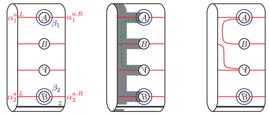
Figure 1.6. Building Heegaard diagrams for mapping cylinders. Left: a Heegaard diagram for the identity map of the torus. Center: the sub-surface $F^{\circ}(\mathcal{Z}_{L})$ and a dashed curve $\gamma$ on $F^{\circ}(\mathcal{Z}_{L})$. Right: a Heegaard diagram for a Dehn twist around $\gamma$. This figure is adapted from [LOT10a, Figure LABEL:LOT2:fig:Build-HD].

Exercise 1.11.

In this exercise we explain how to produce arced Heegaard diagrams for mapping cylinders. This algorithm is explained in somewhat more detail in [LOT10a, Section LABEL:LOT2:sec:DiagramsForAutomorphisms].

1. Show that the arced Heegaard diagram on the left of Figure 1.6 represents the mapping cylinder of the identity map (of the pointed matched circle for a torus). Generalize this to give a diagram for the identity map of any pointed matched circle. (See Figure 5.7 for the standard arced Heegaard diagram for the identity map of another pointed matched circle.)

2. Let $\phi\nobreak\mskip 2.0mu\mathpunct{}\nonscript\mkern-3.0mu{:}\penalty 300\mskip 6.0mu plus 1.0muF(\mathcal{Z}_{L})\to F(\mathcal{Z}_{R})$ be a strongly based homeomorphism. Recall from Construction 1.12 that a neighborhood $F^{\circ}_{L}$ of the graph $\Gamma_{L}$ is identified with $F^{\circ}(\mathcal{Z}_{L})$. Start with the identity Heegaard diagram for $F(\mathcal{Z}_{L})$, and apply the homeomorphism $\phi$ to the $\alpha_{i}^{a,L}\subset F^{\circ}_{L}$. (See Figure 1.6 for an example.) Prove: the result is an arced Heegaard diagram for $\phi$.

Exercise 1.12.

There is a unique pointed matched circle representing the once-punctured torus.

1. List several different pointed matched circles representing the once-punctured genus $2$ surface.

2. Show that the set of matched circles representing the once-punctured genus $k$ surface is in bijection with the set of gluing patterns for the $4k$-gon giving the genus $k$ surface.

Exercise 1.13.

Prove that $\mathcal{A}(-\mathcal{Z})$ is the opposite algebra to $\mathcal{A}(\mathcal{Z})$.

Exercise 1.14.

Let $\mathcal{Z}$ be the split pointed matched circle for a surface of genus $k$, as illustrated in Figure 5.1 (page 5.1). Give a path algebra description of $\mathcal{A}(\mathcal{Z},-k+1)$, similar to Formula (1.18).

Similarly, let $\mathcal{Z}$ be the antipodal pointed matched circle for a surface of genus $k$, i.e., the pointed matched circle in which $a_{i}$ is matched to $a_{i+2k}$ ($i=1,\dots,2k$). Give a path algebra description of $\mathcal{A}(\mathcal{Z},-k+1)$, similar to Formula (1.18). (For a solution to this part, see [LOT13, Example LABEL:faith:eg:antipodal].)

Lecture 2 Modules associated to bordered $3$-manifolds

2.1. Brief review of the cylindrical setting for Heegaard Floer homology

2.1.1. A quick review of the original formulation of Heegaard Floer homology

We start by recalling the definition of Heegaard Floer homology in the closed setting [OSz04d], as well as a “cylindrical” reformulation of the definition [Lip06]; this reformulation will be useful for defining the bordered Floer invariants.

Fix a pointed Heegaard diagram $\mathcal{H}=(\Sigma,{\boldsymbol{\alpha}},{\boldsymbol{\beta}},z)$ (in the sense of [OSz04d]) for a closed $3$-manifold $Y$. Associated to $\mathcal{H}$ are various Heegaard Floer homology groups; as noted in the previous lecture, bordered Floer homology (so far) relates to the technically simplest of these, $\widehat{\mathit{HF}}(Y)$. The group $\widehat{\mathit{HF}}(Y)$ is defined as follows. Suppose $\Sigma$ has genus $g$. Choosing a complex structure $j_{\Sigma}$ on $\Sigma$ makes the symmetric product

$$\operatorname{Sym}^{g}(\Sigma)=\overbrace{\Sigma\times\dots\times\Sigma}^{g\text{ copies}}/S_{g}$$

into a smooth—in fact, Kähler—manifold. (This is not obvious.) Writing ${\boldsymbol{\alpha}}=\{\alpha_{1},\dots,\alpha_{g}\}$ and ${\boldsymbol{\beta}}=\{\beta_{1},\dots,\beta_{g}\}$, the tori $\alpha_{1}\times\dots\times\alpha_{g},\beta_{1}\times\dots\times\beta_{g}\subset\Sigma^{\times g}$ project to embedded tori $T_{\alpha}$ and $T_{\beta}$ in $\operatorname{Sym}^{g}(\Sigma)$. Each of $T_{\alpha}$ and $T_{\beta}$ is totally real; in fact, it was shown in [Per08] that for an appropriate choice of Kähler form the tori $T_{\alpha}$ and $T_{\beta}$ are Lagrangian. Then, $\widehat{\mathit{HF}}(Y)$ is the Lagrangian Floer homology of $(T_{\alpha},T_{\beta})$ inside $\operatorname{Sym}^{g}(\Sigma\setminus\{z\})$.

In a little more detail, $\widehat{\mathit{HF}}(Y)$ is the homology of a chain complex $(\widehat{\mathit{CF}}(Y),\partial)$. $\widehat{\mathit{CF}}(Y)$ is the free ${\mathbb{F}_{2}}$-vector space generated by $T_{\alpha}\cap T_{\beta}$. The differential $\partial\nobreak\mskip 2.0mu\mathpunct{}\nonscript\mkern-3.0mu{:}\penalty 300\mskip 6.0mu plus 1.0mu\widehat{\mathit{CF}}(Y)\to\widehat{\mathit{CF}}(Y)$ is defined by counting holomorphic disks of the following kind. Given $\mathbf{x},\mathbf{y}\in T_{\alpha}\cap T_{\beta}$ we consider the space of maps $\mathbb{D}^{2}\to\operatorname{Sym}^{g}(\Sigma\setminus\{z\})$ such that:

• $-i$ maps to $\mathbf{x}$.

• $+i$ maps to $\mathbf{y}$.

• $\{p\in\partial\mathbb{D}^{2}\mid\Re(p)>0\}$ maps to $T_{\alpha}$.

• $\{p\in\partial\mathbb{D}^{2}\mid\Re(p)<0\}$ maps to $T_{\beta}$.

\begin{overpic}[tics=10,height=144.54pt]{WhitneyDisks}\put(66.0,5.0){$\mathbf{x}$}\put(66.0,70.0){$\mathbf{y}$}\put(91.0,36.0){${\color[rgb]{1,0,0}T_{\alpha}}$}\put(1.0,36.0){${\color[rgb]{0,0,1}T_{\beta}}$}\put(89.0,54.0){$\operatorname{Sym}^{g}(\Sigma)$}\end{overpic}

Figure 2.1. Boundary conditions for Whitney disks.

See Figure 2.1. Such disks are called Whitney disks. Let ${\mathcal{B}}(\mathbf{x},\mathbf{y})$ denote the space of Whitney disks from $\mathbf{x}$ to $\mathbf{y}$. Further:

• Let $\pi_{2}(\mathbf{x},\mathbf{y})$ denote the set of homotopy classes of Whitney disks, i.e., the set of path components in ${\mathcal{B}}(\mathbf{x},\mathbf{y})$.

• Let $\widetilde{\mathcal{M}}(\mathbf{x},\mathbf{y})\subset{\mathcal{B}}(\mathbf{x},\mathbf{y})$ denote the space of holomorphic Whitney disks.

The space $\widetilde{\mathcal{M}}(\mathbf{x},\mathbf{y})$ decomposes according to elements of $\pi_{2}(\mathbf{x},\mathbf{y})$:

$$\widetilde{\mathcal{M}}(\mathbf{x},\mathbf{y})=\coprod_{B\in\pi_{2}(\mathbf{x},\mathbf{y})}\widetilde{\mathcal{M}}^{B}(\mathbf{x},\mathbf{y})$$

If $\widetilde{\mathcal{M}}(\mathbf{x},\mathbf{y})$ is transversally cut-out, each space $\widetilde{\mathcal{M}}^{B}(\mathbf{x},\mathbf{y})$ is a smooth manifold whose dimension is given by a number $\mu(B)$ called the Maslov index of $B$. There is an $\mathbb{R}$-action on both ${\mathcal{B}}(\mathbf{x},\mathbf{y})$ and $\widetilde{\mathcal{M}}(\mathbf{x},\mathbf{y})$ by translation in the source (thought of as an infinite strip). Let $\mathcal{M}^{B}(\mathbf{x},\mathbf{y})=\widetilde{\mathcal{M}}^{B}(\mathbf{x},\mathbf{y})/\mathbb{R}$. Finally, the differential on $\widehat{\mathit{CF}}(Y)$ is given by

(2.1) $$\partial(\mathbf{x})=\sum_{\mathbf{y}\in T_{\alpha}\cap T_{\beta}}\sum_{\begin{subarray}{c}B\in\pi_{2}(\mathbf{x},\mathbf{y})\\ \mu(B)=1\end{subarray}}\bigl{(}\#\mathcal{M}^{B}(\mathbf{x},\mathbf{y})\bigr{)}\mathbf{y}.$$

(Here, $\#$ denotes the modulo-2 count of points.) Under certain assumptions on $\mathcal{H}$, called admissibility, this count is guaranteed to be finite, so $\partial$ is well-defined. Moreover:

Theorem 2.2.

[OSz04d] For any suitably generic choice of almost-complex structure, the map $\partial$ satisfies $\partial^{2}=0$. Moreover, the homology $\widehat{\mathit{HF}}(Y)=H_{*}(\widehat{\mathit{CF}}(Y),\partial)$ is an invariant of $Y$.

2.1.2. The cylindrical reformulation

Before proceeding to bordered Floer homology, it will be helpful to have a mild reformulation of the definition of $\widehat{\mathit{HF}}$. It is based on the tautological correspondence between maps from $\mathbb{D}^{2}$ to $\operatorname{Sym}^{g}(\Sigma)$ and multi-valued functions from $\mathbb{D}^{2}$ to $\Sigma$:

Holomorphic maps $\mathbb{D}^{2}\to\operatorname{Sym}^{g}(\Sigma)$	$\longleftrightarrow$ ​	Diagrams
		with $u_{\Sigma}$, $u_{\mathbb{D}}$ holomorphic,
		$u_{\mathbb{D}}$ a $g$-fold branched cover.

One direction is easy: given a diagram as on the right, consider the map $\mathbb{D}^{2}\to\operatorname{Sym}^{g}(\Sigma)$ given by mapping $p$ to the $g$-tuple $u_{\Sigma}(u_{\mathbb{D}}^{-1}(p))$. The other direction is not hard, either; see, for instance, [Lip06, Section 13].

In light of the tautological correspondence, we can reformulate $\widehat{\mathit{HF}}$ in terms of maps to $\Sigma\times\mathbb{D}^{2}$. It will be convenient later to view $\mathbb{D}^{2}\setminus\{\pm i\}$ as a strip $[0,1]\times\mathbb{R}$. Then:

• Generators of $\widehat{\mathit{CF}}(Y)$ correspond to $g$-tuples of points $\mathbf{x}=\{x_{i}\}_{i=1}^{g}$ with $x_{i}\in\alpha_{i}\cap\beta_{\sigma(i)}$ for some $\sigma\in S_{g}$. These generators can be thought of as $g$-tuples of chords $\mathbf{x}\times[0,1]\subset\Sigma\times[0,1]$, connecting ${\boldsymbol{\alpha}}\times\{1\}$ and ${\boldsymbol{\beta}}\times\{0\}$.

• The differential counts embedded holomorphic maps

  (2.3) $$u\nobreak\mskip 2.0mu\mathpunct{}\nonscript\mkern-3.0mu{:}\penalty 300\mskip 6.0mu plus 1.0mu(S,\partial S)\to\bigl{(}(\Sigma\setminus\{z\})\times[0,1]\times\mathbb{R},({\boldsymbol{\alpha}}\times\{1\}\times\mathbb{R})\cup({\boldsymbol{\beta}}\times\{0\}\times\mathbb{R})\bigr{)}.$$

  modulo translation in $\mathbb{R}$. Here, $S$ is a Riemann surface with boundary and punctures on its boundary. The punctures are divided into $+$ punctures and $-$ punctures. Near the $-$ punctures, $u$ is asymptotic to $\mathbf{x}\times[0,1]\times\{-\infty\}$ and near the $+$ punctures $u$ is asymptotic to $\mathbf{y}\times[0,1]\times\{+\infty\}$.

In the cylindrical setting, the set of homotopy classes $\pi_{2}(\mathbf{x},\mathbf{y})$ of Whitney disks becomes the set of homology classes (in a suitable sense) of maps as in Formula 2.3. (Philosophically, this is related to the Dold-Thom theorem that $\pi_{k}(\operatorname{Sym}^{\infty}(X))\cong H_{k}(X)$.)

We have been suppressing almost-complex structures. In order to achieve transversality, one typically perturbs the complex structure $j_{\Sigma}\times j_{\mathbb{D}}$ on $\Sigma\times[0,1]\times\mathbb{R}$ to a more generic almost-complex structure $J$. In this cylindrical setting, it is important to ensure that translation in $\mathbb{R}$ remains $J$-holomorphic. Some other conditions which are necessary or convenient are given in [Lip06, Section 1].

Remark 2.4.

It would have been more consistent with conventions in contact homology to consider $\mathbb{R}\times[0,1]\times\Sigma$ rather that $\Sigma\times[0,1]\times\mathbb{R}$.

2.2. Holomorphic curves and Reeb chords

Now consider a bordered Heegaard diagram $\mathcal{H}=(\Sigma,{\boldsymbol{\alpha}}^{a},{\boldsymbol{\alpha}}^{c},{\boldsymbol{\beta}},z)$. Rather than viewing $\Sigma$ as a compact surface-with-boundary, attach a cylindrical end $\mathbb{R}\times S^{1}$ to $\partial\Sigma$; and extend the $\alpha$-arcs ${\boldsymbol{\alpha}}^{a}$ in a translation-invariant way to $\mathbb{R}\times S^{1}$. (Topologically, this is the same as simply deleting $\partial\Sigma$; but if one is paying attention to the symplectic form and almost-complex structure then there is a difference.) We abuse notation, using the same notation $\Sigma$ and ${\boldsymbol{\alpha}}^{a}$ for the versions with cylindrical ends. We will still consider holomorphic maps as in Formula (2.3); but now there is a third source of non-compactness, $\partial\Sigma$, and these maps can have asymptotics there as well.

We start with the asymptotics at $\pm\infty$. A term for the asymptotics at $\pm\infty$:

Definition 2.5.

By a generator we mean a $g$-tuple $\mathbf{x}\subset{\boldsymbol{\alpha}}\cap{\boldsymbol{\beta}}$ which has one point on each $\alpha$-circle, one point on each $\beta$-circle, and at most one point on each $\alpha$-arc.

We consider holomorphic curves disjoint from a neighborhood of $z$. It follows from this and the fact that only the $\alpha$-arcs touch $\partial\Sigma$ that the asymptotics at $\partial\Sigma$ are of the form $\rho_{i}\times(1,t_{i})$, where $\rho_{i}$ is a chord in $\partial\Sigma\setminus\{z\}$ with boundary on ${\boldsymbol{\alpha}}^{a}$. We collect these curves into moduli spaces. Let $\widetilde{\mathcal{M}}(\mathbf{x},\mathbf{y};\rho_{1},\dots,\rho_{n})$ denote the moduli space of embedded holomorphic maps as in Formula (2.3) where:

• $S$ is a surface with boundary and punctures on its boundary. Of these punctures, $g$ are labeled $-$, $g$ are labeled $+$, and the rest are labeled $e$.

• $\mathbf{x}$ and $\mathbf{y}$ are generators.

• at the punctures labeled $-$, $u$ is asymptotic to $\mathbf{x}\times[0,1]\times\{-\infty\}$.

• at the punctures labeled $+$, $u$ is asymptotic to $\mathbf{y}\times[0,1]\times\{+\infty\}$.

• at the punctures labeled $e$, $u$ is asymptotic to the chords $\rho_{i}\times(1,t_{i})\in\partial\Sigma\times\{1\}\times\mathbb{R}$. Moreover, we require that $t_{1}<t_{2}<\cdots<t_{n}$.

There is an $\mathbb{R}$-action on $\widetilde{\mathcal{M}}(\mathbf{x},\mathbf{y};\rho_{1},\dots,\rho_{n})$ by translation in the target; let

$$\mathcal{M}(\mathbf{x},\mathbf{y};\rho_{1},\dots,\rho_{n})=\widetilde{\mathcal{M}}(\mathbf{x},\mathbf{y};\rho_{1},\dots,\rho_{n})/\mathbb{R}.$$

We call the chords $\rho$ Reeb chords; they are Reeb chords for the contact structure on $S^{1}=\partial\Sigma$. This comes from thinking of the setup as related to a Morse-Bott case of (relative) symplectic field theory. The asymptotic boundary is then $(\partial\Sigma\times[0,1]\times\mathbb{R},\partial{\boldsymbol{\alpha}}^{a}\times\{1\}\times\mathbb{R})$, and we are in the Levi-flat case of, e.g., [BEH⁺03].

As in the closed case, the space of maps of the form just described naturally decomposes into homology classes; see [LOT08, Section LABEL:LOT1:sec:homology-classes-generators]. To keep notation consistent with the closed case, we let $\pi_{2}(\mathbf{x},\mathbf{y})$ denote the set of homology classes of maps connecting $\mathbf{x}$ to $\mathbf{y}$; note that we do not specify the Reeb chords here. Then

$$\mathcal{M}(\mathbf{x},\mathbf{y};\rho_{1},\dots,\rho_{n})=\coprod_{B\in\pi_{2}(\mathbf{x},\mathbf{y})}\mathcal{M}^{B}(\mathbf{x},\mathbf{y};\rho_{1},\dots,\rho_{n}).$$

As in the closed case, we have been suppressing the almost-complex structure $J$ from the discussion; the interested reader is referred to [LOT08, Section LABEL:LOT1:sec:curves-in-sigma]. For a generic choice of $J$, each of the spaces $\mathcal{M}^{B}(\mathbf{x},\mathbf{y};\rho_{1},\dots,\rho_{n})$ is a manifold whose dimension is given by a number $\operatorname{ind}(B;\rho_{1},\dots,\rho_{n})-1$. The notation $\operatorname{ind}$ stands for index: as is usual for holomorphic curves, the dimension is given by the index of the linearized $\overline{\partial}$-operator. One can give an explicit formula for $\operatorname{ind}(B;\rho_{1},\dots,\rho_{n})$; see [LOT08, Section LABEL:LOT1:sec:expected-dimensions].

The next natural thing to talk about, from an analytic perspective, is what the compactifications of $\mathcal{M}^{B}(\mathbf{x},\mathbf{y};\rho_{1},\dots,\rho_{n})$ look like. We defer this discussion to Lecture 3, and instead turn to the definition of the bordered invariant $\widehat{\mathit{CFD}}(Y)$.

2.3. The definition of $\widehat{\mathit{CFD}}$

2.3.1. Reeb chords and algebra elements

Before defining $\widehat{\mathit{CFD}}(\mathcal{H})$ we need one more piece of notation. Let $\mathcal{Z}=(Z,{\mathbf{a}},M,z)$ be a pointed matched circle and $\rho$ a chord in $Z\setminus\{z\}$ with boundary in ${\mathbf{a}}$. Orienting $\rho$ according to the orientation of $Z$ and identifying ${\mathbf{a}}=\{1,\dots,4k\}$, the chord $\rho$ has an initial point $i$ and a terminal point $j$. Write

(2.6) $$a(\rho)=\sum_{\begin{subarray}{c}S\subset\underline{4k}\\ i\in S\end{subarray}}(S,S\setminus\{i\}\cup\{j\},\phi_{S})$$

where $\phi_{S}(i)=j$ and $\phi_{S}|_{S\setminus i}=\mathbb{I}$, and the sum is only over $S$’s so that $S$ and $S\setminus\{i\}\cup\{j\}$ are $M$-admissible. That is, $a(\rho)$ is the union of a strand from $i$ to $j$ and any admissible set of horizontal strands. A somewhat trivial example is given by Exercise 1.9.

2.3.2. The definition of $\widehat{\mathit{CFD}}$

Fix a bordered Heegaard diagram $\mathcal{H}=(\Sigma,{\boldsymbol{\alpha}}^{a},{\boldsymbol{\alpha}}^{c},{\boldsymbol{\beta}},z)$ with boundary $\mathcal{Z}$. We will define a left dg module $\widehat{\mathit{CFD}}(\mathcal{H})$ over $\mathcal{A}(-\mathcal{Z})$ (where, as usual, $-$ denotes orientation reversal). The module $\widehat{\mathit{CFD}}(\mathcal{H})$ will lie over $\mathcal{A}(-\mathcal{Z},0)$, in the sense that the other summands $\mathcal{A}(-\mathcal{Z},i)$, $i\neq 0$, of $\mathcal{A}(-\mathcal{Z})$ act trivially on $\widehat{\mathit{CFD}}(\mathcal{H})$.

Let $\mathfrak{S}(\mathcal{H})$ denote the set of generators for $\mathcal{H}$. Given a generator $\mathbf{x}\in\mathfrak{S}(\mathcal{H})$, let $I(S)$ denote the set of $\alpha$-arcs which are disjoint from $\mathbf{x}$. Then $I(S)$ corresponds to a set of matched pairs in $-\mathcal{Z}$, and hence, by Exercise 1.10, to an indecomposable idempotent of $\mathcal{A}(-\mathcal{Z})$. As a (left) module, define

$$\widehat{\mathit{CFD}}(\mathcal{H})=\bigoplus_{\mathbf{x}\in\mathfrak{S}(\mathcal{H})}\mathcal{A}(-\mathcal{Z})\cdot I(S).$$

It remains to define the differential on $\widehat{\mathit{CFD}}(\mathcal{H})$. For $\mathbf{x}\in\mathfrak{S}(\mathcal{H})$ define

(2.7) $$\partial(\mathbf{x})=\sum_{\mathbf{y}\in\mathfrak{S}(\mathcal{H})}\sum_{n\geq 0}\sum_{(\rho_{1},\dots,\rho_{n})}\sum_{B\mid\operatorname{ind}(B,\rho_{1},\dots,\rho_{n})=1}\bigl{(}\#\mathcal{M}^{B}(\mathbf{x},\mathbf{y};\rho_{1},\dots,\rho_{n})\bigr{)}a(-\rho_{1})\cdots a(-\rho_{n})\mathbf{y}.$$

Here, the minus signs are included because $\widehat{\mathit{CFD}}$ is a module over $\mathcal{A}(-\mathcal{Z})$ rather than $\mathcal{A}(\mathcal{Z})$; $-\rho$ is the chord $\rho$ but viewed as running in the opposite direction (i.e., as a chord in $-\mathcal{Z}$).

Extend the differential to the rest of $\widehat{\mathit{CFD}}(Y)$ by the Leibniz rule. This completes the definition of $\widehat{\mathit{CFD}}(Y)$.

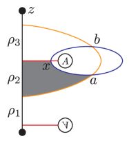
Figure 2.2. A Heegaard diagram for a solid torus, and some holomorphic curves in it. The circles labeled $A$ indicate a handle. The shaded regions in the second through fourth figures indicate the domains giving $a\in\partial(b)$, $\rho_{3}x\in\partial b$, and $\rho_{2}a\in\partial x$, respectively.

Example 2.8.

Consider the bordered Heegaard diagram in Figure 2.2. We have labeled the three length-1 Reeb chords; notice that we have ordered them in the opposite of the order induced by the orientation of $\partial\mathcal{H}$, because we are thinking of the algebra $\mathcal{A}(-\partial\mathcal{H})$. The module $\widehat{\mathit{CFD}}(\mathcal{H})$ has three generators, $x$, $a$ and $b$. With notation as in Formula 1.18, the idempotents are given by

$$I(x)=\iota_{1}\qquad\qquad I(a)=\iota_{0}\qquad\qquad I(b)=\iota_{0}$$

The differentials are given by

$$\partial(b) =a+\rho_{3}x$$

$$\partial(x) =\rho_{2}a$$

$$\partial(a) =0.$$

Each of these differentials comes from a disk mapped to $\Sigma\times[0,1]\times\mathbb{R}$; the projections of these disks to $\Sigma$ (their domains—see Definition 2.9) are indicated in the figure. Since $\rho_{3}\rho_{2}=0$, $\partial^{2}=0$.

2.3.3. Finiteness conditions

As in the closed case, the definition of $\widehat{\mathit{CFD}}$ (Formula (2.7)) only makes sense if the sums involved are finite. To ensure finiteness, we add assumptions on the Heegaard diagram $\mathcal{H}$, analogous to admissibility in the closed case:

Definition 2.9.

Given a homology class $B\in\pi_{2}(\mathbf{x},\mathbf{y})$, the projection of $B$ to $\Sigma$ defines a cellular $2$-chain with respect to the cellulation of $\Sigma$ given by ${\boldsymbol{\alpha}}\cup{\boldsymbol{\beta}}$. This $2$-chain is called the domain of $B$, and determines $B$. A non-trivial class $B$ is called positive if its local multiplicities are all non-negative. The domains of homology classes $B\in\pi_{2}(\mathbf{x},\mathbf{x})$ are called periodic domains. The set of periodic domains does not depend on $\mathbf{x}$.

The Heegaard diagram $\mathcal{H}$ is called provincially admissible if it has no positive periodic domains which have multiplicity $0$ everywhere along $\partial\Sigma$.

The Heegaard diagram $\mathcal{H}$ is called admissible if it has no positive periodic domains.

Lemma 2.10.

[LOT08, Lemma LABEL:LOT1:lem:finite-typeD] If $\mathcal{H}$ is provincially admissible then the sums in Formula (2.7) are finite. Moreover, if $\mathcal{H}$ is admissible then the operator $\partial$ is nilpotent in the following sense. Consider sequences of generators $(\mathbf{x}_{1},\mathbf{x}_{2},\dots,\mathbf{x}_{n})$ such that $\mathbf{x}_{i+1}$ occurs in $\partial\mathbf{x}_{i}$ with nonzero coefficient. If $\mathcal{H}$ is admissible then there is a universal bound on the length of such sequences.

The proof of Lemma 2.10 is not hard; it is an adaptation of the proof of the corresponding fact from the closed case [OSz04d, Lemma 4.14]. The nilpotency condition in Lemma 2.10 guarantees that $\widehat{\mathit{CFD}}(\mathcal{H})$ is projective (or rather, $\mathcal{K}$-projective in the sense of, e.g., [BL94]). It is not particularly relevant until we start taking tensor products, e.g. in the statement of Theorem 1.17.

Theorem 2.11.

[LOT08, Proposition LABEL:LOT1:prop:typeD-d2] Let $\mathcal{H}$ be a provincially admissible Heegaard diagram. Then $\widehat{\mathit{CFD}}(\mathcal{H})$ is a differential module.

The only nontrivial thing to check is that $\partial^{2}=0$. The proof involves studying the boundaries of $1$-dimensional moduli spaces; we will sketch it in the next lecture.

2.4. The surgery exact triangle

Recall that Heegaard Floer homology admits a surgery exact triangle [OSz04c]. Specifically, for a pair $(M,K)$ of a 3-manifold $M$ and a framed knot $K$ in $M$, there is an exact triangle

(2.12)

where $M_{-1}$, $M_{0}$, and $M_{\infty}$ are $-1$, $0$, and $\infty$ surgery on $K$, respectively. As a simple application of bordered Floer theory, we reprove this result.

Consider the three diagrams

(2.13) $$\mathcal{H}_{\infty}:\vbox{\hbox{$\includegraphics[trim=-1.00374pt -1.00374pt -1.00374pt -1.00374pt]{torus-30}$}}\qquad\mathcal{H}_{-1}:\vbox{\hbox{$\includegraphics[trim=-1.00374pt -1.00374pt -1.00374pt -1.00374pt]{torus-20}$}}\qquad\mathcal{H}_{0}:\vbox{\hbox{$\includegraphics[trim=-1.00374pt -1.00374pt -1.00374pt -1.00374pt]{torus-10}$}}$$

(Opposite edges are identified, to give $T^{2}\setminus\mathbb{D}^{2}$. Each diagram has two $\alpha$-arcs and one $\beta$-circle. The numbers indicate which chord, in the notation of Formula (1.18), corresponds to which arc in $\partial\mathcal{H}_{\bullet}$. Note again that the chords are numbered in the opposite of the order induced by the orientation of $\partial\mathcal{H}_{\bullet}$.) A generator for $\widehat{\mathit{CFD}}(\mathcal{H}_{\bullet})$ consists of a single intersection point between the $\beta$-circle in $\mathcal{H}_{\bullet}$ and an $\alpha$-arc. These intersections are labeled above.

The boundary operators on the $\widehat{\mathit{CFD}}(\mathcal{H}_{\bullet})$ (and the relevant domains) are given by

$$\partial r=\underset{\includegraphics[scale={0.5}]{torus-31}}{\rho_{23}r}\qquad\qquad\partial a=\underset{\includegraphics[scale={0.5}]{torus-21}}{\rho_{3}b}+\underset{\includegraphics[scale={0.5}]{torus-22}}{\rho_{1}b}\qquad\qquad\partial b=\underset{\includegraphics[scale={0.5}]{torus-255}}{0}\qquad\qquad\partial n=\underset{\includegraphics[scale={0.5}]{torus-11}}{\rho_{12}n}$$

There is a short exact sequence

$$0\longrightarrow\widehat{\mathit{CFD}}(\mathcal{H}_{\infty})\overset{\varphi}{\longrightarrow}\widehat{\mathit{CFD}}(\mathcal{H}_{-1})\overset{\psi}{\longrightarrow}\widehat{\mathit{CFD}}(\mathcal{H}_{0})\longrightarrow 0$$

where the maps $\phi$ and $\psi$ are given by

$$\varphi(r)=b+\rho_{2}a\qquad\qquad\psi(a)=n\qquad\qquad\psi(b)=\rho_{2}n.$$

Now, the surgery exact triangle follows immediately from the pairing theorem and properties of the derived tensor product.

2.5. The definition of $\widehat{\mathit{CFDD}}$

Suppose $\mathcal{Z}_{L}$ and $\mathcal{Z}_{R}$ are pointed matched circles. We can form their connected sum $\mathcal{Z}_{L}\#\mathcal{Z}_{R}$. There are two natural choice of where to put a basepoint in $\mathcal{Z}_{L}\#\mathcal{Z}_{R}$; let $z$ be a point in one of these places and $w$ a point in the other. Thinking of $z$ as the basepoint, there is an associated algebra $\mathcal{A}(\mathcal{Z}_{L}\#\mathcal{Z}_{R})$. Moreover, there is an algebra homomorphism

$$p\nobreak\mskip 2.0mu\mathpunct{}\nonscript\mkern-3.0mu{:}\penalty 300\mskip 6.0mu plus 1.0mu\mathcal{A}(\mathcal{Z}_{L}\#\mathcal{Z}_{R})\to\mathcal{A}(\mathcal{Z}_{L})\otimes_{\mathbb{F}_{2}}\mathcal{A}(\mathcal{Z}_{R})$$

given by setting to zero any algebra element crossing the extra basepoint $w$.

Now, suppose that $\mathcal{H}$ is an arced Heegaard diagram. Performing surgery on $\mathcal{H}$ along the arc $\mathbf{z}$ gives a bordered Heegaard diagram ${\mathcal{H}}_{dr}$. (Again, there are two choices of where to put the basepoint in ${\mathcal{H}}_{dr}$; choose either.) If the boundary of $\mathcal{H}$ was $\mathcal{Z}_{L}\amalg\mathcal{Z}_{R}$ then the boundary of ${\mathcal{H}}_{dr}$ is $\mathcal{Z}_{L}\#\mathcal{Z}_{R}$.

Associated to ${\mathcal{H}}_{dr}$ is a bordered module $\widehat{\mathit{CFD}}({\mathcal{H}}_{dr})$ over $\mathcal{A}(-(\mathcal{Z}_{L}\#\mathcal{Z}_{R}))$.

Definition 2.14.

With notation as above, let

$$\widehat{\mathit{CFDD}}(\mathcal{H})=\bigl{(}(-\mathcal{A}(\mathcal{Z}_{L}))\otimes_{\mathbb{F}_{2}}(-\mathcal{A}(\mathcal{Z}_{R}))\bigr{)}\otimes_{\mathcal{A}(-(\mathcal{Z}_{L}\#\mathcal{Z}_{R}))}\widehat{\mathit{CFD}}({\mathcal{H}}_{dr}),$$

be the image of the bordered bimodule $\widehat{\mathit{CFD}}({\mathcal{H}}_{dr})$ under the induction functor associated to the homomorphism $p$. Via the correspondence between left-left bimodules over $\mathcal{A}(-\mathcal{Z}_{L})$ and $\mathcal{A}(-\mathcal{Z}_{R})$ and left modules over $\bigl{(}(-\mathcal{A}(\mathcal{Z}_{L}))\otimes_{\mathbb{F}_{2}}(-\mathcal{A}(\mathcal{Z}_{R}))\bigr{)}$, we view $\widehat{\mathit{CFDD}}(\mathcal{H})$ as a left-left bimodule over $\mathcal{A}(-\mathcal{Z}_{L})$ and $\mathcal{A}(-\mathcal{Z}_{R})$.

Of course, this definition can be unpacked to define $\widehat{\mathit{CFDD}}(\mathcal{H})$ directly in terms of intersection points and holomorphic curves; doing so is Exercise 2.8.

2.6. Exercises

Exercise 2.1.

There is a unique almost-complex structure $\operatorname{Sym}^{g}(j_{\Sigma})$ on $\operatorname{Sym}^{g}(\Sigma)$ so that the projection map $(\Sigma^{\times g},j_{\Sigma}^{\times g})\to(\operatorname{Sym}^{g}(\Sigma),\operatorname{Sym}^{g}(j_{\Sigma}))$ is holomorphic. In the tautological correspondence of Section 2.1.2, show that if $u_{\Sigma}$ and $u_{\mathbb{D}}$ are holomorphic then the map $\mathbb{D}^{2}\to\operatorname{Sym}^{g}(\Sigma)$, $p\mapsto u_{\Sigma}(u_{\mathbb{D}}^{-1}(p))$ is holomorphic with respect to $\operatorname{Sym}^{g}(j_{\Sigma})$.

Exercise 2.2.

Consider the Heegaard diagrams of Section 2.4. Replacing the blue ($\beta$) curve in the diagrams $\mathcal{H}_{\bullet}$ by a circle of slope $p/q$ gives a bordered Heegaard diagram $\mathcal{H}_{p/q}$ for a $p/q$-framed solid torus. It is fairly easy to compute the invariants $\widehat{\mathit{CFD}}(\mathcal{H}_{p/q})$ for these diagrams; compute some.

For any triple of rational numbers $(p_{1}/q_{1},p_{2}/q_{2},p_{3}/q_{3})$ (with $p_{i},q_{i}$ relatively prime) such that $p_{1}+p_{2}+p_{3}=q_{1}+q_{2}+q_{3}=0$ there is a corresponding surgery triangle; check this for some other examples.

Figure 2.3. Heegaard diagrams for mapping class group elements. Genus $2$ diagrams for $\tau_{\mu}$, $\tau_{\mu}^{-1}$, $\tau_{\lambda}$ and $\tau_{\lambda}^{-1}$ are shown. In each of the four diagrams, there are three generators in the $i=0$ summand. (This figure is drawn from [LOT09, Figure A.2].)

Exercise 2.3.

Compute $\operatorname{Mor}(\widehat{\mathit{CFD}}(\mathcal{H}_{p/q}),\widehat{\mathit{CFD}}(\mathcal{H}_{r/s}))$ for a few choices of $p,q,r,s$. For example, $\operatorname{Mor}(\widehat{\mathit{CFD}}(\mathcal{H}_{\infty}),\widehat{\mathit{CFD}}(\mathcal{H}_{-1}))$ has generators $(r\mapsto b)$, $(r\mapsto\rho_{23}b)$ and $(r\mapsto\rho_{2}a)$. The differentials are given by

$$\partial(r\mapsto b) =(r\mapsto\rho_{23}b)$$

$$\partial(r\mapsto\rho_{2}a) =(r\mapsto\rho_{23}b).$$

In particular, the homology of this $\operatorname{Mor}$ complex is $1$-dimensional.

Recall that $\widehat{\mathit{HF}}(L(p,q))\cong(\mathbb{F}_{2})^{p}$ , and $\widehat{\mathit{HF}}(S^{2}\times S^{1})\cong(\mathbb{F}_{2})^{2}$; check that your answers are consistent with this.

Exercise 2.4.

We explain the type DD bimodule $\widehat{\mathit{CFDD}}(\mathbb{I},0)$ associated to the mapping cylinder for the identity map of $F(\mathcal{Z})$. The notation is somewhat cumbersome, as $\widehat{\mathit{CFDD}}(\mathbb{I},0)$ has two commuting left actions by $\mathcal{A}(T^{2},0)$. We write one of these copies of $\mathcal{A}(T^{2},0)$ in the notation of Formula (1.18), and the other in the same way but with $\sigma$’s in place of $\rho$’s and $\eta$’s in place of $\iota$’s. Then, the bimodule $\widehat{\mathit{CFDD}}(\mathbb{I},0)$ has two generators, $x$ and $y$, with

$$\iota_{0}x=\eta_{0}x=x\qquad\qquad\iota_{1}y=\eta_{1}y=y$$

and differential given by

(2.15) $$\begin{split}\partial x&=(\rho_{1}\sigma_{3}+\rho_{3}\sigma_{1}+\rho_{123}\sigma_{123})\otimes y\\ \partial y&=(\rho_{2}\sigma_{2})\otimes x.\end{split}$$

(Compare [LOT08, Section LABEL:LOT1:sec:dd-of-id].)

Verify that for the modules $\widehat{\mathit{CFD}}(\mathcal{H}_{\bullet})$ of Section 2.4, $\operatorname{Mor}(\widehat{\mathit{CFDD}}(\mathbb{I},0),\cdot)$ acts as the identity. That is, check that

$$\operatorname{Mor}_{\mathcal{A}(T^{2},0)}(\widehat{\mathit{CFDD}}(\mathbb{I},0),\widehat{\mathit{CFD}}(\mathcal{H}_{0}))\simeq\widehat{\mathit{CFD}}(\mathcal{H}_{0}),$$

and similarly for $\mathcal{H}_{-1}$, $\mathcal{H}_{\infty}$. (You will have to use the equivalence of categories between left $\mathcal{A}(T^{2},0)$-modules and right $\mathcal{A}(T^{2},0)$-modules coming from the fact that $\mathcal{A}(T^{2},0)\cong\mathcal{A}(T^{2},0)^{\mathrm{op}}$. Note that this isomorphism exchanges $\rho_{1}$ and $\rho_{3}$.)

Remark 2.16.

There are two non-equivalent notions of the $\operatorname{Mor}$ complex above, depending on how one treats the other algebra action on $\widehat{\mathit{CFDD}}(\mathbb{I},0)$. The exercise will be true with either notion. See [LOT11a, Theorems 5 and 6] for an example where this distinction matters.

Remark 2.17.

It is sometimes convenient to encode the operations in Formula (2.15) by:

$$\leavevmode\hbox to156.69pt{\vbox to58.73pt{\text{[drawing]}}}. x y {\rho_{1}\sigma_{3}+\rho_{3}\sigma_{1}+\rho_{123}\sigma_{123}} {\rho_{2}\sigma_{2}} x y {\rho_{1}\sigma_{3}+\rho_{3}\sigma_{1}+\rho_{123}\sigma_{123}} {\rho_{2}\sigma_{2}}$$

This way of encoding operations on DD bimodules will be used in Exercise 2.6.

Exercise 2.5.

Note that the identity for $\operatorname{Mor}$ is the $\mathcal{A}$-bimodule $\mathcal{A}$. In spite of the computations in Exercise 2.4, $\widehat{\mathit{CFDD}}(\mathbb{I})\not\simeq\mathcal{A}(T^{2},0)$. Check this two ways:

• Directly. (Think about the rank of the homologies.)

• By finding a module $M$ over $\mathcal{A}(T^{2},0)$ so that $\widehat{\mathit{CFDD}}(\mathbb{I})\otimes_{\mathcal{A}(T^{2},0)}M\not\simeq M$. (Or, you can use $\operatorname{Mor}(\widehat{\mathit{CFDD}}(\mathbb{I}),M)$ if you prefer.)

Exercise 2.6.

Let $\tau_{\mu}$ and $\tau_{\lambda}$ denote the Dehn twists of the torus along a meridian and a longitude, respectively. Heegaard diagrams for the mapping cylinders of $\tau_{\mu}$ and $\tau_{\lambda}$ are shown in Figure 2.3. With notation as in Remark 2.17, the type DD bimodules associated to these Dehn twists and their inverses are given by

Convince yourself that these bimodules satisfy $\partial^{2}=0$. Compute $\operatorname{Mor}(\widehat{\mathit{CFDD}}(\tau_{\mu}),\mathcal{H}_{0})$ and $\operatorname{Mor}(\widehat{\mathit{CFDD}}(\tau_{\lambda}),\mathcal{H}_{0})$. Compare the results with the answers you computed in Exercise 2.2.

Exercise 2.7.

Up to Heegaard moves, there are some symmetries relating the diagrams in Figure 2.3. How are these symmetries reflected in the bimodules in Exercise 2.6?

Exercise 2.8.

Unpack the definition of $\widehat{\mathit{CFDD}}$ from Section 2.5 to give a direct definition, avoiding the induction functor.

Lecture 3 Analysis underlying the invariants and the pairing theorem

3.1. Broken flows in the cylindrical setting

As a warm-up, we begin this lecture by discussing the proof that $\partial^{2}=0$ for the cylindrical picture for Heegaard Floer homology. We start with an example. Consider the Heegaard diagram for $S^{3}$ shown in Figure 3.1. There are five generators, labeled $a$, $b$, $c$, $d$ and $e$. The differentials are given by

$$\partial(a)=b+c\qquad\qquad\partial(b)=\partial(c)=d\qquad\qquad\partial(d)=0\qquad\qquad\partial(e)=b+c.$$

(Remember that we are working with ${\mathbb{F}_{2}}$-coefficients.)

Consider the moduli space $\mathcal{M}(a,d)$ of curves connecting $a$ to $d$. This moduli space consists of holomorphic maps

$$u\nobreak\mskip 2.0mu\mathpunct{}\nonscript\mkern-3.0mu{:}\penalty 300\mskip 6.0mu plus 1.0mu(\mathbb{D}^{2}\setminus\{\pm i\})\to\Sigma\times[0,1]\times\mathbb{R}.$$

Suppose we are working with the almost-complex structure $j_{\Sigma}\times j_{\mathbb{D}}$. Then there are projection maps $\pi_{\Sigma}\nobreak\mskip 2.0mu\mathpunct{}\nonscript\mkern-3.0mu{:}\penalty 300\mskip 6.0mu plus 1.0mu\Sigma\times[0,1]\times\mathbb{R}\to\Sigma$ and $\pi_{\mathbb{D}}\nobreak\mskip 2.0mu\mathpunct{}\nonscript\mkern-3.0mu{:}\penalty 300\mskip 6.0mu plus 1.0mu\Sigma\times[0,1]\times\mathbb{R}\to[0,1]\times\mathbb{R}$, and $u$ being holomorphic is equivalent to $\pi_{\Sigma}\circ u$ and $\pi_{\mathbb{D}}\circ u$ being holomorphic.

The map $\pi_{\mathbb{D}}\circ u$ is a $1$-fold branched cover, i.e., an isomorphism; up to translation, there is a unique such isomorphism.

A short argument using the Riemann mapping theorem shows that the map $\pi_{\Sigma}\circ u$ is determined by the image of $\partial\mathbb{D}^{2}$. Figure 3.1 shows two possibilities for $\pi_{\Sigma}(u(\partial\mathbb{D}^{2}))$. Note the branch point on $\alpha_{1}$ or $\beta_{1}$. The whole moduli space is determined by where the branch point lies; so, $\mathcal{M}(a,d)$ is an (open) interval. The ends of $\mathcal{M}(a,d)$ occur when the branch point approaches $b$ or $c$.

\begin{overpic}[tics=10,width=346.89731pt]{S3moduli} \put(51.0,40.0){$a$} \put(53.0,43.0){$b$} \put(54.0,50.0){$d$} \put(53.0,58.0){$c$} \put(51.0,64.5){$e$} \put(48.0,34.0){{\color[rgb]{0,0,1}$\beta$}} \put(23.0,57.0){{\color[rgb]{1,0,0}$\alpha$}} \put(50.0,80.0){$z$} \put(46.0,53.0){$p_{2}$} \put(64.0,50.0){$p_{1}$} \end{overpic}

Figure 3.1. An unnecessarily complicated diagram for $S^{3}$. In the two pictures on the bottom we have indicated the image $\pi_{\Sigma}(u(\partial\mathbb{D}^{2}))$ for two typical elements of $\mathcal{M}(a,d)$. The thick black segments indicate cuts.

We want to describe the limiting objects. In the ordinary setting for Morse theory, these would be broken flows. In this setting, they are multi-story holomorphic buildings. We see this as follows.

Consider a sequence of curves $u_{i}$ approaching the end of $\mathcal{M}(a,d)$ where the branch point approaches $c$. Notice the points $p_{1},p_{2}\in\Sigma$ shown in Figure 3.1. Consider the points $q_{1}=(\pi_{\Sigma}\circ u_{i})^{-1}(p_{1})$ and $q_{2}=(\pi_{\Sigma}\circ u_{i})^{-1}(p_{2})$ in $\mathbb{D}^{2}$. The points $(\pi_{\mathbb{D}}\circ u_{i})(q_{1})$ and $(\pi_{\mathbb{D}}\circ u_{i})(q_{2})$ in $[0,1]\times\mathbb{R}$ are getting farther and farther apart. Indeed, from the point of view of $q_{1}$, half of the holomorphic curve is heading towards $\Sigma\times[0,1]\times\{+\infty\}$, while from the point of view of $q_{2}$, half of the holomorphic curve is heading towards $\Sigma\times[0,1]\times\{-\infty\}$. So, the limiting object has two “stories”: the part of the limit containing $q_{1}$ and the part of the limit containing $q_{2}$. More formally:

Definition 3.1.

An $\ell$-story holomorphic building connecting $\mathbf{x}$ to $\mathbf{y}$ consists of a sequence of holomorphic curves $u_{i}\in\mathcal{M}(\mathbf{x}_{i},\mathbf{x}_{i+1})$, $i=1,\dots,\ell$, with $\mathbf{x}_{1}=\mathbf{x}$ and $\mathbf{x}_{\ell+1}=\mathbf{y}$.

Each holomorphic building carries a homology class in $\pi_{2}(\mathbf{x},\mathbf{y})$, by adding up (concatenating) the homology classes of its stories.

We should now give a topology on the space of holomorphic buildings, to say precisely what it means for a sequence of one-story buildings, i.e., elements of $\mathcal{M}(a,d)$, to converge to a multi-story building. Instead, however, we refer the reader to [BEH⁺03].

The main structural result is:

Theorem 3.2.

Suppose that $B\in\pi_{2}(\mathbf{x},\mathbf{y})$ has $\mu(B)=2$. Let $\overline{\mathcal{M}}{}{}^{B}(\mathbf{x},\mathbf{y})$ denote the space of $1$- or $2$-story holomorphic buildings connecting $\mathbf{x}$ to $\mathbf{y}$ in the homology class $B$. Then for a generic choice of almost-complex structure, $\overline{\mathcal{M}}{}{}^{B}(\mathbf{x},\mathbf{y})$ is a compact $1$-dimensional manifold-with-boundary. The boundary of $\overline{\mathcal{M}}{}{}^{B}(\mathbf{x},\mathbf{y})$ consists exactly of the $2$-story holomorphic buildings connecting $\mathbf{x}$ to $\mathbf{y}$ in the homology class $B$.

In the cylindrical formulation, this is [Lip06, Corollary 7.2]; the analogous result for Heegaard Floer homology in the non-cylindrical setting was proved in [OSz04d]. (Both proofs are relatively modest adaptations of standard holomorphic curve techniques.)

To conclude the warm-up, we recall that $\partial^{2}=0$ follows from Theorem 3.2 by a standard argument:

Corollary 3.3.

Let $\mathcal{H}$ be an admissible Heegaard diagram for a closed $3$-manifold. Then the differential $\partial$ on $\widehat{\mathit{CF}}(\mathcal{H})$ satisfies $\partial^{2}=0$.

Proof.

The proof involves the usual looking at ends of one-dimensional moduli spaces, as is familiar in Floer homology:

$$\partial(\mathbf{x}) =\sum_{\mathbf{y}\in\mathfrak{S}(\mathcal{H})}\sum_{\begin{subarray}{c}B_{1}\in\pi_{2}(\mathbf{x},\mathbf{y})\\ \mu(B_{1})=1\end{subarray}}\bigl{(}\#\mathcal{M}^{B_{1}}(\mathbf{x},\mathbf{y})\bigr{)}\mathbf{y}$$

$$\partial^{2}(x) =\sum_{\mathbf{y}\in\mathfrak{S}(\mathcal{H})}\sum_{\begin{subarray}{c}B_{1}\in\pi_{2}(\mathbf{x},\mathbf{y})\\ \mu(B_{1})=1\end{subarray}}\bigl{(}\#\mathcal{M}^{B_{1}}(\mathbf{x},\mathbf{y})\bigr{)}\partial(\mathbf{y})$$

$$=\sum_{\mathbf{y},\mathbf{z}\in\mathfrak{S}(\mathcal{H})}\sum_{\begin{subarray}{c}B_{1}\in\pi_{2}(\mathbf{x},\mathbf{y})\\ \mu(B_{1})=1\end{subarray}}\sum_{\begin{subarray}{c}B_{2}\in\pi_{2}(\mathbf{y},\mathbf{z})\\ \mu(B_{2})=1\end{subarray}}\bigl{(}\#\mathcal{M}^{B_{1}}(\mathbf{x},\mathbf{y})\bigr{)}\bigl{(}\#\mathcal{M}^{B_{2}}(\mathbf{y},\mathbf{z})\bigr{)}\mathbf{z}$$

$$=\sum_{\mathbf{z}\in\mathfrak{S}(\mathcal{H})}\sum_{\begin{subarray}{c}B\in\pi_{2}(\mathbf{x},\mathbf{z})\\ \mu(B)=2\end{subarray}}\bigl{(}\#\partial\mathcal{M}^{B}(\mathbf{x},\mathbf{z})\bigr{)}\mathbf{z}$$

$$=0.$$

Most of this is just manipulation of symbols; the key point is the fourth equality, which uses Theorem 3.2. The last equality follows from the fact that a $1$-dimensional manifold-with-boundary has an even number of ends. (The assumption about admissibility is used to ensure that the sums involved at each stage are finite.) ∎

3.2. The codimension-one boundary: statement

To prove that $\partial^{2}=0$ for $\widehat{\mathit{CFD}}$ we need to investigate the boundary of the $1$-dimensional moduli spaces, analogously to Theorem 3.2. So, fix a bordered Heegaard diagram $\mathcal{H}=(\Sigma,{\boldsymbol{\alpha}}^{c},{\boldsymbol{\alpha}}^{a},{\boldsymbol{\beta}})$. As above, we can have breaking at $\pm\infty$, giving multi-story holomorphic buildings; but now there are two other sources of non-compactness:

1. The manifold $\Sigma$ has a cylindrical end, giving another direction in which curves in $\Sigma\times[0,1]\times\mathbb{R}$ can break.

2. In the moduli space $\mathcal{M}^{B}(\mathbf{x},\mathbf{y};\rho_{1},\dots,\rho_{n})$ we had Reeb chords $\rho_{i}\times(1,t_{i})$ where $t_{1}<t_{2}<\dots<t_{n}$. This can degenerate when $t_{i+1}-t_{i}\to 0$.

(There is overlap between the two cases.)

Degenerations of type (1) lead to the analogue of $2$-story holomorphic buildings, but in the “horizontal”, i.e., $\Sigma$, direction. In principle, one can have degenerations in both the vertical ($\mathbb{R}$) and horizontal ($\Sigma$) directions at once. We called the resulting objects holomorphic combs [LOT08, Definition LABEL:LOT1:def:comb]. In codimension $1$, the kinds of combs that can appear are quite limited, so rather than giving the general story we will simply explain these cases.

By east $\infty$ we mean $\mathbb{R}\times(\partial\Sigma)\times[0,1]\times\mathbb{R}$; this is the symplectic manifold that one sees at the (“horizontal”) end of $\Sigma$. Note that there are projection maps

$$\pi_{\Sigma} \nobreak\mskip 2.0mu\mathpunct{}\nonscript\mkern-3.0mu{:}\penalty 300\mskip 6.0mu plus 1.0mu\mathbb{R}\times(\partial\Sigma)\times[0,1]\times\mathbb{R}\to\mathbb{R}\times(\partial\Sigma)$$

$$\pi_{\mathbb{D}} \nobreak\mskip 2.0mu\mathpunct{}\nonscript\mkern-3.0mu{:}\penalty 300\mskip 6.0mu plus 1.0mu\mathbb{R}\times(\partial\Sigma)\times[0,1]\times\mathbb{R}\to[0,1]\times\mathbb{R}$$

$$t \nobreak\mskip 2.0mu\mathpunct{}\nonscript\mkern-3.0mu{:}\penalty 300\mskip 6.0mu plus 1.0mu\mathbb{R}\times(\partial\Sigma)\times[0,1]\times\mathbb{R}\to\mathbb{R},$$

where $t$ is projection onto the second (last) $\mathbb{R}$-factor. Degenerations of type (1) lead to pairs $(u,v)$ where $u$ is a curve in $\Sigma\times[0,1]\times\mathbb{R}$ of the kind we have been considering and $v$ is a curve at east $\infty$, i.e., a holomorphic map

$$v\nobreak\mskip 2.0mu\mathpunct{}\nonscript\mkern-3.0mu{:}\penalty 300\mskip 6.0mu plus 1.0mu(S,\partial S)\to(\mathbb{R}\times(\partial\Sigma)\times[0,1]\times\mathbb{R},\mathbb{R}\times({\boldsymbol{\alpha}}\cap\partial\Sigma)\times\{1\}\times\mathbb{R}).$$

Here, $S$ is a surface with boundary and punctures on the boundary. Each puncture is labeled either $e$ or $w$. Near each $e$ puncture, $v$ is asymptotic to some $\{\infty\}\times\rho_{i}\times(1,t_{i})$ where $\rho_{i}$ is a chord in $\partial\Sigma$ and $t_{i}\in\mathbb{R}$. Similarly, near each $w$ puncture, $v$ is asymptotic to some $\{-\infty\}\times\rho_{i}\times(1,t_{i})$.

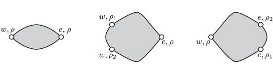
Figure 3.2. Sources of curves at east $\infty$. Left: a trivial component. Center: a join component. Right: a split component. This is [LOT08, Figure LABEL:LOT1:fig:trivial_split_join_domain].

It follows from the boundary conditions and asymptotics that for each component of $v$, the map $\pi_{\mathbb{D}}\circ v$ is, in fact, constant. This makes describing holomorphic curves at east $\infty$ relatively straightforward. Three kinds of curves will play special roles in studying $\widehat{\mathit{CFD}}$:

• A trivial component is a disk in $\mathbb{R}\times(\partial\Sigma)\times[0,1]\times\mathbb{R}$ which is invariant under translation in the first $\mathbb{R}$-factor. It follows that a trivial component has one $w$ punctures and one $e$ puncture, and is asymptotic to the same chord $\rho$ at both punctures.

• A join component is a disk in $\mathbb{R}\times(\partial\Sigma)\times[0,1]\times\mathbb{R}$ with two $w$ punctures and one $e$ puncture. At the two $w$ punctures the curve is asymptotic to chords $\rho_{1}$ and $\rho_{2}$ and at the $e$ puncture the curve is asymptotic to a chord $\rho$. With respect to the cyclic ordering of the punctures $(\rho,\rho_{1},\rho_{2})$ around the boundary of the disk (see Figure 3.2), the terminal endpoint of $\rho_{2}$ is the initial endpoint of $\rho_{1}$; and $\rho=\rho_{2}\cup\rho_{1}$.

  A join curve is the disjoint union of one join component and finitely many trivial components.

• Roughly, a split component is the mirror of a join component. In more detail, a split component is a disk in $\mathbb{R}\times(\partial\Sigma)\times[0,1]\times\mathbb{R}$ with one $w$ punctures and two $e$ puncture. At the two $e$ punctures the curve is asymptotic to chords $\rho_{1}$ and $\rho_{2}$ and at the $w$ puncture the curve is asymptotic to a chord $\rho$. With respect to the cyclic ordering of the punctures $(\rho,\rho_{1},\rho_{2})$ around the boundary of the disk (see Figure 3.2), the terminal endpoint of $\rho_{1}$ is the initial endpoint of $\rho_{2}$; and $\rho=\rho_{1}\cup\rho_{2}$.

  For our purposes, a split curve is the disjoint union of one split component and finitely many trivial components. (If we were also interested in $\widehat{\mathit{CFA}}$, we would have to allow more than one split component in a split curve.)

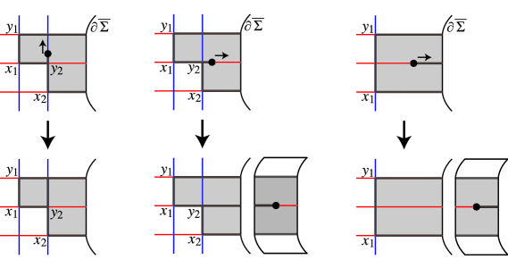
Figure 3.3. Examples of three kinds of codimension $1$ degenerations. The large black dot represents a boundary branch point of $\pi_{\Sigma}\circ u$. Left: degenerating into a two-story building. Center: degenerating a join curve. Right: degenerating a split curve. The diagrams show the projection of the curve in $\Sigma\times[0,1]\times\mathbb{R}$ to $\Sigma$. This figure is adapted from [LOT08, Figure LABEL:LOT1:fig:degen_examples].

Figure 3.3 gives examples of degenerating a join curve and a split curve at east $\infty$, as well as breaking into a two-story holomorphic building.

Remark 3.4.

In studying $\widehat{\mathit{CFA}}$, a third kind of curve at east $\infty$, called a shuffle curve, is also important. See [LOT08, Section LABEL:LOT1:sec:curves_at_east_infinity] for a discussion of shuffle curves.

Theorem 3.5.

Suppose that $\operatorname{ind}(B;\rho_{1},\dots,\rho_{n})=2$. Then the ends of the moduli space $\mathcal{M}^{B}(\mathbf{w},\mathbf{y};\rho_{1},\dots,\rho_{n})$ consist exactly of the following configurations:

1. Two-story holomorphic buildings, i.e.,

   $$\bigcup_{i=0}^{n}\,\bigcup_{\mathbf{x}\in\mathfrak{S}(\mathcal{H})}\,\bigcup_{\begin{subarray}{c}B_{1}\in\pi_{2}(\mathbf{w},\mathbf{x})\\ B_{2}\in\pi_{2}(\mathbf{x},\mathbf{y})\\ B_{1}*B_{2}=B\end{subarray}}\mathcal{M}^{B_{1}}(\mathbf{w},\mathbf{x};\rho_{1},\dots,\rho_{i})\times\mathcal{M}^{B_{2}}(\mathbf{x},\mathbf{y};\rho_{i+1},\dots,\rho_{n}).$$

2. Collapses of levels, i.e., curves $u$ as in the definition of $\mathcal{M}^{B}(\mathbf{w},\mathbf{y};\rho_{1},\dots,\rho_{n})$ except that the $t$-coordinates of $\rho_{i}$ and $\rho_{i+1}$ are equal. Moreover, either:

   1. the set of (one or two) $\alpha$-arcs containing $\partial\rho_{i}$ must be disjoint from the set of (one or two) $\alpha$-arcs containing $\partial\rho_{i+1}$, or

   2. the initial endpoint of $\rho_{i}$ is the same as the final endpoint of $\rho_{i+1}$.

3. Join curve degenerations, i.e., pairs $(u,v)$ where $u$ is a curve like those in

   $$\mathcal{M}^{B}(\mathbf{w},\mathbf{y};\rho_{1},\dots,\rho^{\prime}_{i},\rho^{\prime\prime}_{i},\rho_{i+1},\dots,\rho_{n})$$

   except that the $t$-coordinates of $\rho^{\prime}_{i}$ and $\rho^{\prime\prime}_{i}$ are equal; and $v$ is a join curve with $w$ asymptotics $\rho_{1},\dots,\rho^{\prime}_{i},\rho^{\prime\prime}_{i},\dots,\rho_{n}$ and $e$ asymptotics $\rho_{1},\dots,\rho_{i},\dots,\rho_{n}$. In particular, $\rho_{i}=\rho^{\prime\prime}_{i}\cup\rho^{\prime}_{i}$. Moreover:

   • The $\alpha$-arc containing the terminal end of $\rho^{\prime\prime}_{i}$ is distinct from the $\alpha$-arcs containing the initial and terminal ends of $\rho_{i}$.

   • The $t$-coordinates of the $w$ asymptotics of $v$ agree with the $t$-coordinates of the $e$ asymptotics of $u$.

4. Split curve degenerations, i.e., pairs $(u,v)$ where

   $$u\in\mathcal{M}^{B}(\mathbf{w},\mathbf{y};\rho_{1},\dots,\rho_{i}\cup\rho_{i+1},\dots,\rho_{n})$$

   and $v$ is a split curve with $w$ asymptotics $\rho_{1},\dots,(\rho_{i}\cup\rho_{i+1}),\dots,\rho_{n}$ and $e$ asymptotics $\rho_{1},\dots,\rho_{i},\rho_{i+1},\dots,\rho_{n}$. Moreover, the $t$-coordinates of the $w$ asymptotics of $v$ agree with the $t$-coordinates of the $e$ asymptotics of $u$.

   In particular, the space of such pairs $(u,v)$ can be canonically identified with $\mathcal{M}^{B}(\mathbf{w},\mathbf{y};\rho_{1},\dots,\rho_{i}\cup\rho_{i+1},\dots,\rho_{n})$.

This is a combination of [LOT08, Theorem LABEL:LOT1:thm:master_equation] and [LOT08, Lemma LABEL:LOT1:lemma:collision-is-composable].

As in most of holomorphic curve theory, the key ingredients in the proof of Theorem 3.5 are:

• A transversality statement: for generic almost-complex structures, the relevant moduli spaces are transversally cut out. For curves in $\Sigma\times[0,1]\times\mathbb{R}$ this is [LOT08, Proposition LABEL:LOT1:prop:transversality]; for curves at east $\infty$, it is [LOT08, Proposition LABEL:LOT1:prop:east_transversality]. Because we are not able to perturb the complex structure at east $\infty$, less transversality holds for curves at east $\infty$ than one might like. (Specifically, we can not always ensure that the evaluation maps at the punctures are transverse to the diagonal.)

• A compactness statement: sequences of holomorphic curves in $\Sigma\times[0,1]\times\mathbb{R}$ converge to holomorphic combs. This is [LOT08, Proposition LABEL:LOT1:prop:compactness].

• Various gluing statements. Because of the Morse-Bott nature of the asymptotics at east $\infty$ and transversality issues for curves at east $\infty$, these statements become somewhat intricate. See [LOT08, Section LABEL:LOT1:sec:combs-gluing].

• An analysis of which of the possible degenerations can occur in codimension-$1$. See [LOT08, Sections LABEL:LOT1:sec:degenerations-holomorphic-curves and LABEL:LOT1:sec:embedded-degen].

There is one more ingredient, because we are working with embedded curves:

• A computation of the index of the $\overline{\partial}$ operator shows that sequences of embedded curves converge to embedded curves. Philosophically, this is related to the adjunction formula. See [LOT08, Section LABEL:LOT1:sec:expected-dimensions] for further discussion.

Remark 3.6.

The fact that $\pi_{\mathbb{D}}$ is constant on each component of a curve at east $\infty$ suggests that we have lost some information in our formulation of the limiting objects. One could recover this information by rescaling while taking the limit. Specifically, suppose a sequence of holomorphic curves $u_{i}$ converges to a pair $(u,v)$, where $v\nobreak\mskip 2.0mu\mathpunct{}\nonscript\mkern-3.0mu{:}\penalty 300\mskip 6.0mu plus 1.0muT\to\mathbb{R}\times(\partial\Sigma)\times[0,1]\times\mathbb{R}$ is a curve at east $\infty$. Fix a marked point $p_{i}$ on each $u_{i}$ converging to a marked point $p$ on $u$. In taking the limit, rescale the map $\pi_{\mathbb{D}}\circ u_{i}$ on a neighborhood of $p_{i}$ so that $d_{p_{i}}(\pi_{\mathbb{D}}\circ u_{i})$ has norm $1$. With some work, one thus obtains a rescaled version of $\pi_{\mathbb{D}}\circ v$ in the form of a map $T\to\{x+iy\in\mathbb{C}\mid x\leq 1\}$.

The moduli spaces at east $\infty$ are sufficiently simple that this refined limiting procedure turns out not to be necessary to construct the bordered invariants; but it seems more relevant to constructing a bordered version of $\mathit{HF}^{\pm}$.

3.3. $\partial^{2}=0$ on $\widehat{\mathit{CFD}}$

With the codimension-$1$ boundary in hand, we are now ready to prove that $\widehat{\mathit{CFD}}$ is a dg module.

Theorem 3.7.

[LOT08, Proposition LABEL:LOT1:prop:typeD-d2] Fix a provincially admissible bordered Heegaard diagram $\mathcal{H}$. Then for a generic choice of almost-complex structure, the differential $\partial$ on $\widehat{\mathit{CFD}}(\mathcal{H})$ satisfies $\partial^{2}=0$.

Sketch of proof..

It suffices to show that for each generator $\mathbf{w}\in\mathfrak{S}(\mathcal{H})$, $\partial^{2}(\mathbf{w})=0$. We have

$$\partial^{2}(\mathbf{w}) =\partial\Bigl{(}\sum_{\begin{subarray}{c}\mathbf{y}\in\mathfrak{S}(\mathcal{H})\\ (\rho_{1},\dots,\rho_{n})\\ B\in\pi_{2}(\mathbf{w},\mathbf{y})\end{subarray}}\bigl{(}\#\mathcal{M}^{B}(\mathbf{w},\mathbf{y};\rho_{1},\dots,\rho_{n})\bigr{)}a(-\rho_{1})\cdots a(-\rho_{n})\mathbf{y}\Bigr{)}$$

$$=\sum_{\begin{subarray}{c}\mathbf{x}\in\mathfrak{S}(\mathcal{H})\\ (\rho_{1},\dots,\rho_{i})\\ B_{1}\in\pi_{2}(\mathbf{w},\mathbf{x})\end{subarray}}\sum_{\begin{subarray}{c}\mathbf{y}\in\mathfrak{S}(\mathcal{H})\\ (\rho_{i+1},\dots,\rho_{n})\\ B_{2}\in\pi_{2}(\mathbf{w},\mathbf{x})\end{subarray}}\bigl{(}\#\mathcal{M}^{B_{1}}(\mathbf{w},\mathbf{x};\rho_{1},\dots,\rho_{i})\bigr{)}\bigl{(}\#\mathcal{M}^{B_{2}}(\mathbf{w},\mathbf{x};\rho_{i+1},\dots,\rho_{n})\bigr{)}$$

$$\hskip 216.81pt\cdot a(-\rho_{1})\cdots a(-\rho_{i})a(-\rho_{i+1})\cdots a(-\rho_{n})\mathbf{y}$$

$$\qquad+\sum_{\begin{subarray}{c}\mathbf{x}\in\mathfrak{S}(\mathcal{H})\\ (\rho_{1},\dots,\rho_{n})\\ B\in\pi_{2}(\mathbf{w},\mathbf{x})\end{subarray}}\bigl{(}\#\mathcal{M}^{B}(\mathbf{w},\mathbf{x};\rho_{1},\dots,\rho_{n})\bigr{)}a(-\rho_{1})\cdots d(a_{i})\cdots a(-\rho_{n})\mathbf{x}.$$

(There is some possibly confusing re-indexing: in the second line we have replaced $n\to i$, $\mathbf{y}\to\mathbf{x}$, and $B\to B_{1}$. In the last line we use the same notation as in the first line, however.)

The sum in the second line corresponds exactly to the $2$-story holomorphic buildings, degeneration (1) in Theorem 3.5. The sum in the last line corresponds to the split curve degenerations, degeneration (4) in Theorem 3.5.

It remains to see that the other ends of the $1$-dimensional moduli spaces cancel in pairs. Indeed, it is easy to see that Case 2(item:degen:collapsea) ends of $\mathcal{M}^{B}(\mathbf{w},\mathbf{y};\rho_{1},\dots,\rho_{n})$ correspond to Case 2(item:degen:collapsea) ends of $\mathcal{M}^{B}(\mathbf{w},\mathbf{y};\rho_{1},\dots,\rho_{i+1},\rho_{i},\dots,\rho_{n})$; and Case 2(item:degen:collapseb) ends of $\mathcal{M}^{B}(\mathbf{w},\mathbf{y};\rho_{1},\dots,\rho_{n})$ correspond to join curve ends of $\mathcal{M}^{B}(\mathbf{w},\mathbf{y};\rho_{1},\dots,\rho_{i}\cup\rho_{i+1},\dots,\rho_{n})$. This completes the proof. ∎

3.4. Deforming the diagonal, $\widehat{\mathit{CFA}}$ and the pairing theorem

Our goals for the rest of the lecture are two-fold:

1. Define the invariant $\widehat{\mathit{CFA}}(Y)$ associated to a bordered $3$-manifold.

2. Prove the pairing theorem, Theorem 1.17.

We will do this in the opposite order: we will start proving Theorem 1.17, and $\widehat{\mathit{CFA}}$ will appear naturally. The material in this section is drawn from [LOT08, Chapter LABEL:LOT1:chap:tensor-prod], to which we refer the reader for further details.

\begin{overpic}[tics=10]{cut_HD} \put(48.0,10.0){$Z$} \put(20.0,2.0){$\mathcal{H}_{1}$} \put(78.0,2.0){$\mathcal{H}_{2}$} \put(48.0,0.0){$\mathcal{H}$} \put(31.0,18.0){$a$} \put(29.0,41.0){$b$} \put(72.0,23.0){$s$} \put(49.0,49.0){$z$} \end{overpic}

Figure 3.4. Splitting a closed Heegaard diagram. The bordered Heegaard diagrams $\mathcal{H}_{1}$ and $\mathcal{H}_{2}$ are glued along the circle $Z\subset\mathcal{H}$.

So, fix bordered Heegaard diagrams $\mathcal{H}_{1}$, $\mathcal{H}_{2}$ with $\partial\mathcal{H}_{1}=\mathcal{Z}=-\partial\mathcal{H}_{2}$ and let $\mathcal{H}=\mathcal{H}_{1}\cup_{\partial}\mathcal{H}_{2}$. (See Figure 3.4.) We want to understand $\widehat{\mathit{CF}}(\mathcal{H})$ in terms of invariants of $\mathcal{H}_{1}$ and $\mathcal{H}_{2}$.

On the level of generators, this is trivial: a generator $\mathbf{x}\in\widehat{\mathit{CF}}(\mathcal{H})$ corresponds to a pair of generators $(\mathbf{x}_{1},\mathbf{x}_{2})$ for $\mathcal{H}_{1}$ and $\mathcal{H}_{2}$ so that the $\alpha$-arcs occupied by $\mathbf{x}_{1}$ are complementary to the $\alpha$-arcs occupied by $\mathbf{x}_{2}$. So, if we define $I_{A}(\mathbf{x}_{1})$ to be the idempotent in $\mathcal{A}(\mathcal{Z})$ corresponding to the $\alpha$-arcs occupied by $\mathbf{x}_{1}$—this is the opposite of $I(\mathbf{x})$ as defined in Section 2.3.2—and let

$$\widehat{\mathit{CFA}}(\mathcal{H}_{1})={\mathbb{F}_{2}}\langle\mathfrak{S}(\mathcal{H}_{1})\rangle,$$

with $I_{A}(\mathbf{x}_{1})\mathbf{x}_{1}=\mathbf{x}_{1}$, so other indecomposable idempotents kill $\mathbf{x}_{1}$, then we have

(3.8) $$\widehat{\mathit{CFA}}(\mathcal{H}_{1})\otimes_{\mathcal{A}(\mathcal{Z})}\widehat{\mathit{CFD}}(\mathcal{H}_{2})$$

as ${\mathbb{F}_{2}}$-vector spaces. Note that we have not defined an $\mathcal{A}(\mathcal{Z}_{1})$-module structure on $\widehat{\mathit{CFA}}(\mathcal{H}_{1})$ yet: Equation 3.8 uses only the action of the idempotents and the fact that $\widehat{\mathit{CFD}}(\mathcal{H}_{2})$ is a sum of elementary projective modules.

Holomorphic curves are more complicated.

Let $Z\subset\mathcal{H}$ denote the circle $\partial\mathcal{H}_{1}$. Recall that to define $\widehat{\mathit{CFD}}(\mathcal{H}_{2})$ we attached a cylindrical end to $-Z=\partial\Sigma_{2}$. Correspondingly, to prove the pairing theorem, we consider inserting a long neck into $\Sigma$ along $Z$. That is, fix a complex structure $j_{\Sigma}$ on $\Sigma$ and choose a neighborhood $U$ of $Z$ which is biholomorphic to $[-\epsilon,\epsilon]\times S^{1}$ for some $\epsilon>0$. Let $j_{\Sigma}^{R}$ denote the result of replacing $U$ by $[-R,R]\times S^{1}$.

Let $R_{i}\in\mathbb{R}$ be a sequence with $R_{i}\to\infty$, and suppose $u_{i}\in\mathcal{M}^{B}(\mathbf{x},\mathbf{y})$ is a sequence of holomorphic curves with respect to $j_{\Sigma}^{R_{i}}\times j_{\mathbb{D}}$. We are interested in the limit of the sequence $\{u_{i}\}$. Modulo some technicalities, this is the kind of limit studied in symplectic field theory; the limiting objects have the following form:

Definition 3.9.

A matched holomorphic curve is a pair of curves

$$(u_{1},u_{2})\in\mathcal{M}^{B_{1}}(\mathbf{x}_{1},\mathbf{y}_{1};\rho_{1},\dots,\rho_{n})\times\mathcal{M}^{B_{2}}(\mathbf{x}_{2},\mathbf{y}_{2};\rho_{1},\dots,\rho_{n})$$

so that for each $i=1,\dots,n$, the $t$-coordinate at which $u_{1}$ is asymptotic to $\rho_{i}$ is equal to the $t$-coordinate at which $u_{2}$ is asymptotic to $\rho_{i}$.

Equivalently, there is an evaluation map

$$\operatorname{ev}\nobreak\mskip 2.0mu\mathpunct{}\nonscript\mkern-3.0mu{:}\penalty 300\mskip 6.0mu plus 1.0mu\mathcal{M}^{B_{i}}(\mathbf{x}_{i},\mathbf{y}_{i};\rho_{1},\dots,\rho_{n})\to\mathbb{R}^{n-1}$$

which takes a curve asymptotic to $\rho_{1}\times(1,t_{1}),\dots,\rho_{n}\times(1,t_{n})$ to $(t_{2}-t_{1},t_{3}-t_{2},\dots,t_{n}-t_{n-1})$. Then a matched holomorphic curve is a pair $(u_{1},u_{2})$ such that $\operatorname{ev}(u_{1})=\operatorname{ev}(u_{2})$.

Let $\mathcal{M}^{B}(\mathbf{x},\mathbf{y};\infty)$ denote the moduli space of matched holomorphic curves in the homology class $B$. That is,

(3.10) $$\mathcal{M}^{B}(\mathbf{x},\mathbf{y};\infty)=\bigcup_{(\rho_{1},\dots,\rho_{n})}\mathcal{M}^{B_{1}}(\mathbf{x}_{1},\mathbf{y}_{1};\rho_{1},\dots,\rho_{n})\mathbin{{}_{\operatorname{ev}}\mathord{\times}_{\operatorname{ev}}}\mathcal{M}^{B_{2}}(\mathbf{x}_{2},\mathbf{y}_{2};\rho_{1},\dots,\rho_{n}).$$

Here, $\mathbf{x}$ (respectively $\mathbf{y}$) corresponds to the pair of generators $(\mathbf{x}_{1},\mathbf{x}_{2})$ (respectively $(\mathbf{y}_{1},\mathbf{y}_{2})$) and $B_{i}$ is the intersection of $B$ with $\mathcal{H}_{i}$.

Proposition 3.11.

Let $\mathcal{M}^{B}(\mathbf{x},\mathbf{y};R)$ denote the moduli space of holomorphic curves (in $\Sigma\times[0,1]\times\mathbb{R}$, in the homology class $B$) with respect to an appropriate perturbation of the almost-complex structure $j_{\Sigma}^{R}\times j_{\mathbb{D}}$. Suppose that $\mu(B)=1$. Then $\bigcup_{R>0}\mathcal{M}^{B}(\mathbf{x},\mathbf{y};R)$ is a $1$-manifold whose ends as $R\to\infty$ are identified with $\mathcal{M}^{B}(\mathbf{x},\mathbf{y};\infty)$. More precisely, let

$$\mathcal{M}^{B}(\mathbf{x},\mathbf{y};\geq\!R_{0})=\mathcal{M}^{B}(\mathbf{x},\mathbf{y};\infty)\cup\bigcup_{R\geq R_{0}}\mathcal{M}^{B}(\mathbf{x},\mathbf{y};R)$$

Then there is a there is a topology on $\mathcal{M}^{B}(\mathbf{x},\mathbf{y};\geq R_{0})$ and an $R_{0}$ so that $\mathcal{M}^{B}(\mathbf{x},\mathbf{y};\geq R_{0})$ is a compact $1$-manifold with boundary exactly

$$\mathcal{M}^{B}(\mathbf{x},\mathbf{y};\infty)\amalg\mathcal{M}^{B}(\mathbf{x},\mathbf{y};R_{0}).$$

This follows from compactness and gluing arguments, in a fairly standard way.

Corollary 3.12.

Define $\partial_{1}\nobreak\mskip 2.0mu\mathpunct{}\nonscript\mkern-3.0mu{:}\penalty 300\mskip 6.0mu plus 1.0mu\widehat{\mathit{CF}}(\mathcal{H})\to\widehat{\mathit{CF}}(\mathcal{H})$ by

(3.13) $$\partial_{1}(\mathbf{x})=\sum_{\mathbf{y}\in T_{\alpha}\cap T_{\beta}}\sum_{\begin{subarray}{c}B\in\pi_{2}(\mathbf{x},\mathbf{y})\\ \mu(B)=1\end{subarray}}\#\mathcal{M}^{B}(\mathbf{x},\mathbf{y};\infty)\mathbf{y}$$

(cf. Formula (2.1)). Then $H_{*}(\widehat{\mathit{CF}}(\mathcal{H}),\partial_{1})\cong\widehat{\mathit{HF}}(Y)$.

Example 3.14.

Consider the splitting in Figure 3.4. The complex $\widehat{\mathit{CF}}(\mathcal{H})$ has two generators, $\mathbf{x}=\{a,s\}$ and $\mathbf{y}=\{b,s\}$; in the notation above, $\mathbf{x}_{1}=\{a\}$, $\mathbf{x}_{2}=\{s\}$, $\mathbf{y}_{1}=\{b\}$ and $\mathbf{y}_{2}=\{s\}$. The generator $\mathbf{y}$ occurs twice in $\partial(\mathbf{x})$: once from the small bigon region near the left of the diagram and once from the annular region crossing through the circle $Z$. We focus on the second of these contributions, the domain of which is shown in Figure 3.5. (It takes a little work to show that this domain has a holomorphic representative; see Exercise 3.5.)

Now, consider the result of stretching the neck along $Z$. There are two cases, depending on whether the cut goes through $Z$ or not (which in turn depends on the complex structure on $\mathcal{H}$). If the cut does not go through $z$, the resulting matched curve $(u_{1},u_{2})$ has $u_{1}$ a disk with one Reeb chord and $u_{2}$ an annulus with one Reeb chord. (In fact, this case does not occur in the limit; see Exercise 3.6.)

The more interesting case—and the one which actually occurs—is when the cut does pass through $Z$. Then both $u_{1}$ and $u_{2}$ are disks with two Reeb chords on each of their boundaries. The disk $u_{2}$ is rigid, but the disk $u_{1}$ comes in a $1$-parameter family, depending on the length of the cut. There is algebraically one length of cut for which the height difference of the two Reeb chords in $u_{1}$ agrees with the height difference of the Reeb chords in $u_{2}$ (Exercise 3.7).

\begin{overpic}[tics=10,scale={1.5}]{cut_domain} \put(67.0,22.0){$T\to\infty$} \put(68.0,5.0){$T\to 0$} \end{overpic}

Figure 3.5. Splitting an interesting domain. Depending on the complex structure, there are two possible phenomena after splitting: either the cut stays entirely on the right side of the diagram, as in the left picture, or the cut runs through the collapsed circle $Z$, as in the right picture. We have drawn schematic illustrations of the matched holomorphic curves below the two pictures.

Corollary 3.12 is a step in the direction of a pairing theorem: it gives a definition of $\widehat{\mathit{HF}}$ in terms of holomorphic curves in $\Sigma_{1}\times[0,1]\times\mathbb{R}$ and $\Sigma_{2}\times[0,1]\times\mathbb{R}$. But as we saw in Example 3.14, the corollary still has two (related) drawbacks:

1. The moduli spaces we are considering in for $\mathcal{H}_{1}$ and $\mathcal{H}_{2}$ are typically high-dimensional. Indeed, in Formula (3.13), we have

   $$\dim\mathcal{M}^{B_{1}}(\mathbf{x}_{1},\mathbf{y}_{1};\rho_{1},\dots,\rho_{n})+\dim\mathcal{M}^{B_{2}}(\mathbf{x}_{2},\mathbf{y}_{2};\rho_{1},\dots,\rho_{n})=n-1.$$

2. Since we are taking a fiber product of moduli spaces, which curves we want to consider in $\mathcal{H}_{1}$ depends on $\mathcal{H}_{2}$. So, it is not yet obvious how to define independent invariants of $\mathcal{H}_{1}$ and $\mathcal{H}_{2}$ containing the information needed to compute $\partial_{1}$.

To address complaint (2) we could try to formulate an algebra which remembers the chain $\operatorname{ev}_{*}[\mathcal{M}^{B_{1}}(\mathbf{x}_{1},\mathbf{y}_{1};\rho_{1},\dots,\rho_{n})]\in C_{*}(\mathbb{R}^{n-1})$. This is a natural way to try to define a bordered Heegaard Floer invariant, and with enough effort it could probably be made to work. This approach would be far from combinatorial, and is also unnecessarily complicated, as we will now show.

The next step is to deform the fiber product in Formula (3.10):

Definition 3.15.

A $T$-matched holomorphic curve is a pair

$$(u_{1},u_{2})\in\mathcal{M}^{B_{1}}(\mathbf{x}_{1},\mathbf{y}_{1};\rho_{1},\dots,\rho_{n}){\times}\mathcal{M}^{B_{2}}(\mathbf{x}_{2},\mathbf{y}_{2};\rho_{1},\dots,\rho_{n})$$

such that $T\cdot\operatorname{ev}(u_{1})=\operatorname{ev}(u_{2})$. Let $\mathcal{M}^{B}_{T}(\mathbf{x},\mathbf{y};\infty)$ denote the moduli space of $T$-matched holomorphic curves, i.e.,

$$\mathcal{M}^{B}_{T}(\mathbf{x},\mathbf{y};\infty)=\bigcup_{(\rho_{1},\dots,\rho_{n})}\mathcal{M}^{B_{1}}(\mathbf{x}_{1},\mathbf{y}_{1};\rho_{1},\dots,\rho_{n})\mathbin{{}_{T\cdot\operatorname{ev}}\mathord{\times}_{\operatorname{ev}}}\mathcal{M}^{B_{2}}(\mathbf{x}_{2},\mathbf{y}_{2};\rho_{1},\dots,\rho_{n}).$$

So, in particular, a $1$-matched holomorphic curve is just a matched holomorphic curve.

A standard continuation-map argument shows:

Proposition 3.16.

Let $\partial_{T}$ denote the map defined analogously to Formula 2.1 (or Formula 3.13) but using the moduli spaces $\mathcal{M}^{B}_{T}(\mathbf{x},\mathbf{y};\infty)$. Then $H_{*}(\widehat{\mathit{CF}}(\mathcal{H}),\partial_{T})\cong\widehat{\mathit{HF}}(Y)$.

Now, of course, we send $T\to\infty$. Consider a sequence of $T_{i}$-matched curves $(u_{1}^{i},u_{2}^{i})$ with $T_{i}\to\infty$. Suppose that $u_{1}^{i}\in\mathcal{M}^{B_{1}}(\mathbf{x}_{1},\mathbf{y}_{1};(\rho_{1},\dots,\rho_{n}))$. Let $s_{j}^{i}$ be the $\mathbb{R}$–coordinate at which $u_{1}^{i}$ is asymptotic to $\rho_{j}$ and let $t_{j}^{i}$ be the $\mathbb{R}$–coordinate at which $u_{2}^{i}$ is asymptotic to $\rho_{j}$. Then, after passing to a subsequence, for each $\rho_{j}$, either:

• $(s_{j+1}^{i}-s_{j}^{i})\in(0,\infty)$ stays bounded away from $0$ and $(t_{j+1}^{i}-t_{j}^{i})\to\infty$ as $i\to\infty$; or

• $(s_{j+1}^{i}-s_{j}^{i})\to 0$ and $(t_{j+1}^{i}-t_{j}^{i})$ stays bounded as $i\to\infty$.

So, in the limit:

• On the right we have an $\ell$-story holomorphic building (for some $\ell$) $U_{2}^{\infty}=(v_{1},\dots,v_{\ell})$, where $v_{j}\in\mathcal{M}(\mathbf{x}_{1,j},\mathbf{x}_{1,j+1};\rho_{n_{j}},\dots,\rho_{n_{j+1}})$, $\mathbf{x}_{1,j}=\mathbf{x}_{1}$, $\mathbf{x}_{1,\ell+1}=\mathbf{y}_{1}$, $1=n_{1}\leq n_{2}\leq\dots\leq n_{\ell+1}=n$.

• On the left we have a curve $u_{1}^{\infty}$ asymptotic to some sets of Reeb chords ${\boldsymbol{\rho}}_{1},\dots,{\boldsymbol{\rho}}_{\ell}$ at $t$-coordinates $t_{1}<\dots<t_{\ell}\in\mathbb{R}$. Let

  $$\mathcal{M}^{B_{2}}(\mathbf{x}_{2},\mathbf{y}_{2};{\boldsymbol{\rho}}_{1},\dots,{\boldsymbol{\rho}}_{\ell})$$

  denote the moduli space of such curves.

Importantly, there is no longer a matching condition between the curves $u_{1}^{\infty}$ and $U_{2}^{\infty}$.

Example 3.17.

Continuing with Example 3.14 in the case that the cut goes through the neck, as on the right of Figure 3.5, as $T\to\infty$ the $\mathbb{R}$-coordinates of the two Reeb chords in $u_{1}$ come together. (This results in degenerating a split curve at $\partial\Sigma$; we elided this point in the rest of this section.) This is indicated schematically in Figure 3.5.

Now, suppose we turned the diagram $180^{\circ}$. To avoid re-drawing the figure, we can think of this as sending $T\to 0$ instead of $T\to\infty$. In this case, the two chords in Figure 3.5 are pushed farther and farther apart; in the limit, the cut goes all the way through to the $\beta$-curve, giving a $2$-story holomorphic building. Again, this is indicated schematically in Figure 3.5.

Observe that in both cases, the relevant curves are completely determined, i.e., belong to rigid moduli spaces: there is no “cut” left.

Now, associated to a set of Reeb chords ${\boldsymbol{\rho}}$ is an algebra element $a({\boldsymbol{\rho}})$, defined analogously to Equation (2.6); see Exercise 3.9 or [LOT08, Definition LABEL:LOT1:def:arhos]. Define maps

$$m_{i+1}\nobreak\mskip 2.0mu\mathpunct{}\nonscript\mkern-3.0mu{:}\penalty 300\mskip 6.0mu plus 1.0mu\widehat{\mathit{CFA}}(\mathcal{H}_{1})\otimes\mathcal{A}(\mathcal{Z})^{\otimes i} \to\widehat{\mathit{CFA}}(\mathcal{H}_{1})$$

$$m_{i+1}(\mathbf{x};a({\boldsymbol{\rho}}_{1}),\dots,a({\boldsymbol{\rho}}_{i})) =\sum_{\mathbf{y}\in\mathfrak{S}(\mathcal{H}_{1})}\sum_{\begin{subarray}{c}B\in\pi_{2}(\mathbf{x},\mathbf{y})\\ \operatorname{ind}(B,{\boldsymbol{\rho}}_{1},\dots,{\boldsymbol{\rho}}_{i})=1\end{subarray}}\bigl{(}\#\mathcal{M}^{B}(\mathbf{x},\mathbf{y};{\boldsymbol{\rho}}_{1},\dots,{\boldsymbol{\rho}}_{i})\bigr{)}\mathbf{y}.$$

An argument similar to but in some ways easier than the proof of Theorem 3.7 proves:

Theorem 3.18.

For $\mathcal{H}_{1}$ a provincially-admissible Heegaard diagram and $J$ a generic almost-complex structure, the operations $m_{i+1}$ make $\widehat{\mathit{CFA}}(\mathcal{H}_{1})$ into an $A_{\infty}$-module.

The argument above is a sketch of the pairing theorem, Theorem 1.17. Specifically, it follows from the sketch above that

$$\widehat{\mathit{CF}}(\mathcal{H})\simeq\widehat{\mathit{CFA}}(\mathcal{H}_{1})\boxtimes\widehat{\mathit{CFD}}(\mathcal{H}_{2}),$$

where $\boxtimes$ is the model for the tensor product of an $A_{\infty}$-module with a type $D$ structure described in [LOT08, Section LABEL:LOT1:sec:DT].

3.5. Exercises

Exercise 3.1.

In the setting of Section 3.1, use the Riemann mapping theorem to show that the map $\pi_{\Sigma}\circ u$ is determined by the position of the branch point (as claimed), and that there are no other elements of $\mathcal{M}(a,d)$.

Exercise 3.2.

Suppose that $v\nobreak\mskip 2.0mu\mathpunct{}\nonscript\mkern-3.0mu{:}\penalty 300\mskip 6.0mu plus 1.0muS\to\mathbb{R}\times(\partial\Sigma)\times[0,1]\times\mathbb{R}$ is a holomorphic curve at east $\infty$, as discussed in Section 3.2. Show that the restriction of $\pi_{\mathbb{D}}\circ v$ to each component of $S$ is constant.

Exercise 3.3.

Prove: If $\mathbf{x}$ is a generator for $\widehat{\mathit{CFD}}(Y)$, where $\partial Y=F(\mathcal{Z})$ then $I(\mathbf{x})\in\mathcal{A}(\mathcal{Z},0)\subset\mathcal{A}(\mathcal{Z})$. (Hint: this is easy.) What is the corresponding statement for the bimodules $\widehat{\mathit{CFDD}}$ associated to arced cobordisms?

Exercise 3.4.

The differential on the algebra $\mathcal{A}(T^{2},0)$ associated to the torus is trivial. This means that one of the cases in the proof of Theorem 3.7 does not arise if the boundary is a torus. Which one? Why?

Exercise 3.5.

Show that the annular region in Figure 3.5 is the domain of a holomorphic map $S\to\Sigma\times[0,1]\times\mathbb{R}$, in two ways:

1. By adapting the argument from [OSz04d, Lemma 9.3].

2. By using handleslide invariance of Heegaard Floer homology. (After performing the right handleslide on Figure 3.4, it is easy to compute $\widehat{\mathit{HF}}$.)

Exercise 3.6.

Show that when one stretches the neck in Figure 3.4, as in Example 3.14, the domain in Figure 3.5 must have a cut passing through the neck.

Exercise 3.7.

In Example 3.14 we claimed there is algebraically one length of cut so that the height difference of the two Reeb chords in $u_{1}$ agrees with the height difference of the two Reeb chords in $u_{2}$. (Since we are working with ${\mathbb{F}_{2}}$-coefficients, probably we really meant that there are an odd number of such cut lengths.) Prove this. (Hint: what is the height difference in $u_{1}$ when the cut has length $0$? When the cut goes all the way to the $\beta$-circle?)

Figure 3.6. Degenerating the hexagon. A hexagon in the Heegaard diagram (giving a flow from $\mathbf{x}=\{x_{1},x_{2},x_{3}\}$ to $\mathbf{y}=\{y_{1},y_{2},y_{3}\}$) is divided into three pieces $D_{1}$, $D_{2}$, and $D_{3}$, grouped as $D_{1}$ and $D_{2}\cup D_{3}$. This is [LOT08, Figure LABEL:LOT1:fig:Hexagon].

Exercise 3.8.

Figure 3.6 shows a hexagonal domain connecting $\mathbf{x}=\{x_{1},x_{2},x_{3}\}$ to $\mathbf{y}=\{y_{1},y_{2},y_{3}\}$. Note that this domain always contributes a term of $\mathbf{y}$ in $\partial(\mathbf{x})$. Consider the result of degenerating this domain along the dashed line, and then deforming the diagonal as in Section 3.4. (In the notation of Section 3.4, consider both the case of sending $T\to\infty$ and the case of sending $T\to 0$.) What happens to the holomorphic representative for this domain in the process? How is this encapsulated algebraically? (See [LOT08, Section LABEL:LOT1:sec:tensor-prod-eg] for a detailed discussion of this example.)

Exercise 3.9.

Define $a({\boldsymbol{\rho}})\in\mathcal{A}(\mathcal{Z})$ when ${\boldsymbol{\rho}}$ is a set of chords in $\mathcal{Z}$, no two of which start (respectively end) at points from the same matched pair. (This is a generalization of Formula (2.6), and should be straightforward. See [LOT08, Definition LABEL:LOT1:def:arhos] for a solution.)

Lecture 4 Computing with bordered Floer homology I: knot complements

In this section we will discuss how the torus boundary case of bordered Floer homology can be used to do certain kinds of computations. The main goal is a technique for studying satellite knots, from [LOT08, Chapter LABEL:LOT1:chap:TorusBoundary]. This technique and extensions of it have been used in [Lev12b, Lev12a, Pet09, Hom12].

We start with a review of knot Floer homology [OSz04b, Ras03], mainly to fix notation (Section 4.1). We then discuss how the knot Floer homology of a knot $K$ in $S^{3}$ determines the bordered Floer homology of $S^{3}\setminus K$ (Section 4.2). Finally, we turn this around to use our understanding of bordered Floer homology to study the knot Floer homology of satellites (Section 4.3).

4.1. Review of knot Floer homology

Let $K$ be a knot in $S^{3}$, and let $\mathcal{H}=(\Sigma,{\boldsymbol{\alpha}},{\boldsymbol{\beta}},z,w)$ be a doubly pointed Heegaard diagram for $K$, in the sense of [OSz04b]. (For example, a doubly pointed Heegaard diagram for the trefoil is shown in Figure 4.1.) Associated to $\mathcal{H}$ are various knot Floer homology groups. The most general of these is $\mathit{CFK}^{-}(K)$, which is a filtered chain complex over ${\mathbb{F}_{2}}[U]$. The complex $\mathit{CFK}^{-}(K)$ is freely generated (over ${\mathbb{F}_{2}}[U]$) by $T_{\alpha}\cap T_{\beta}$, the same generators as $\widehat{\mathit{CF}}(\Sigma,{\boldsymbol{\alpha}},{\boldsymbol{\beta}})$. The differential is given by

$$\partial^{-}(\mathbf{x})=\sum_{\mathbf{y}}\,\sum_{\begin{subarray}{c}B\in{\widetilde{\pi}}_{2}(\mathbf{x},\mathbf{y})\\ \mu(B)=1\end{subarray}}\#\bigl{(}\mathcal{M}^{B}(\mathbf{x},\mathbf{y})\bigr{)}U^{n_{w}(B)}\cdot\mathbf{y}.$$

Here, unlike the discussion above, we allow disks to cross the basepoint $z$; we have used the notation ${\widetilde{\pi}}_{2}(\mathbf{x},\mathbf{y})$ rather than $\pi_{2}(\mathbf{x},\mathbf{y})$ to indicate this.

The complex $\mathit{CFK}^{-}(K)$ has an integral grading, called the Maslov grading, which is decreased by one by the differential. We will make no particular reference to this additional structure in the present notes; but it will be convenient (for the purposes of taking Euler characteristic, cf. Equations (4.1) and (4.2) below) to have its parity, as encoded in $(-1)^{M(\mathbf{x})}$. This parity is given as the local intersection number of $T_{\alpha}$ and $T_{\beta}$ at $\mathbf{x}$. (As defined, we have specified a function $\mathfrak{S}(\mathcal{H})\to\{\pm 1\}$ which is well-defined up to overall sign.) Now, the fact that $\partial^{-}$ respects this parity is equivalent to the the statement that if $B\in{\widetilde{\pi}}_{2}(\mathbf{x},\mathbf{y})$ has $\operatorname{ind}(B)=1$, then the local intersection numbers of $T_{\alpha}$ and $T_{\beta}$ at $\mathbf{x}$ and $\mathbf{y}$ are opposite.

The complex $\mathit{CFK}^{-}(K)$ has an Alexander filtration which is uniquely determined up to translation by

$$A(\mathbf{y})-A(\mathbf{x}) =n_{w}(B)-n_{z}(B)$$

$$A(U\cdot\mathbf{y}) =A(\mathbf{y})-1$$

where $B\in\pi_{2}(\mathbf{x},\mathbf{y})$. In other words, a term of the form $U^{n_{w}(B)}\mathbf{y}$ in $\partial^{-}(x)$ has $A(U^{n_{w}(B)}\mathbf{y})=A(\mathbf{x})-n_{z}(B)$.

Let $\mathit{gCFK}^{-}(K)$ denote the associated graded complex to $(\mathit{CFK}^{-}(K),A)$. Explicitly, the differential on $\mathit{gCFK}^{-}(K)$ is defined in the same way as the differential on $\mathit{CFK}^{-}(K)$ except that we no longer allow holomorphic curves to cross the $z$ basepoint. Thus, the chain complex $\mathit{gCFK}^{-}$ splits as a direct sum of complexes, determined by the Alexander grading:

$$\mathit{gCFK}^{-}(K)=\bigoplus_{s\in\mathbb{Z}}\mathit{gCFK}^{-}(K,s).$$

Finally, there is the complex $\widehat{\mathit{CFK}}(K)$ obtained from $\mathit{gCFK}^{-}(K)$ by setting $U=0$. In other words, $\widehat{\mathit{CFK}}(K)$ is generated over ${\mathbb{F}_{2}}$ by $T_{\alpha}\cap T_{\beta}$, and the differential counts holomorphic curves which do not cross $z$ or $w$. Like $\mathit{gCFK}^{-}$, $\widehat{\mathit{CFK}}$ has a direct sum splitting induced by the Alexander grading.

A key property of knot Floer homology is that its graded Euler characteristic is the Alexander polynomial:

(4.1) $$\Delta_{K}(T)=\sum_{s\in\mathbb{Z}}\chi(\widehat{\mathit{CFK}}(K,s))T^{s};$$

and similarly,

(4.2) $$\Delta_{K}(T)/(1-T)=\sum_{s\in\mathbb{Z}}\chi(\mathit{CFK}^{-}(K,s))T^{s}.$$

(Note that the parity of the Maslov grading is used to compute the Euler characteristic. Also, both sides of Formula (4.2) are formal power series.)

The translation indeterminacy in the Alexander grading can then be removed by requiring the graded Euler characteristic of $\widehat{\mathit{CFK}}$ to be the Conway normalized Alexander polynomial (or equivalently $\chi(\widehat{\mathit{CFK}}(K,s))=\chi(\widehat{\mathit{CFK}}(K,-s))$ for all $s\in\mathbb{Z}$); this normalization can also be used to remove the overall indeterminacy in the parity of the Maslov grading.

There is a numerical invariant for knots derived from knot Floer homology, $\tau(K)$, which will appear in Theorem 4.6 below. This is defined with the help of the following observation. There are $U$-non-torsion elements in $H_{*}(\mathit{gCFK}^{-}(K,s))$, i.e., elements $h\in H_{*}(\mathit{gCFK}^{-}(K,s))$ with the property that for all positive integers $m$, $U^{m}h$ is homologically non-trivial. We can consider the maximal $s$ for which $H_{*}(\mathit{gCFK}^{-}(K,s))$ contains $U$-non-torsion elements. Multiplying this $s$ by $-1$ gives the invariant $\tau(K)$.

\begin{overpic}[tics=10,width=346.89731pt]{TrefoilHD_new} \put(52.0,5.0){$a$} \put(54.0,14.5){$b$} \put(51.5,29.5){$c$} \put(46.0,12.0){$z$} \put(55.5,22.0){$w$} \put(48.0,0.0){{\color[rgb]{0,0,1}$\beta$}} \put(29.0,35.0){{\color[rgb]{1,0,0}$\alpha$}} \end{overpic}

Figure 4.1. Doubly pointed Heegaard diagram for the trefoil.

Example 4.3.

Figure 4.1 shows a doubly-pointed Heegaard diagram for the trefoil knot. The chain complex $\mathit{CFK}^{-}(\mathcal{H})$ is given by ${\mathbb{F}_{2}}[U]\langle a,b,c\rangle$. The differential on $\mathit{CFK}^{-}(\mathcal{H})$ is given by

$$\partial^{-}(a) =b \partial^{-}(b) =0 \partial^{-}(c) =Ub.$$

The Alexander filtration is given by $A(a)=1$, $A(b)=0$, $A(c)=-1$.

The differential on $\mathit{gCFK}^{-}(\mathcal{H})$ is given by

$$\partial^{-}_{g}(a) =0 \partial^{-}_{g}(b) =0 \partial^{-}_{g}(c) =Ub.$$

The complex $\widehat{\mathit{CFK}}(\mathcal{H})$ is ${\mathbb{F}_{2}}\langle a,b,c\rangle$, with trivial differential.

\begin{overpic}[tics=10,width=346.89731pt]{Fig8HD} \put(49.0,6.5){$a$} \put(53.0,11.0){$b$} \put(51.0,17.0){$d$} \put(52.5,24.5){$c$} \put(48.5,29.5){$e$} \put(46.0,19.5){$w$} \put(60.0,17.0){$z$} \put(48.0,0.0){{\color[rgb]{0,0,1}$\beta$}} \put(23.0,25.0){{\color[rgb]{1,0,0}$\alpha$}} \end{overpic}

Figure 4.2. Doubly pointed Heegaard diagram for the figure eight knot

Another concrete example is furnished by the Figure 8 knot.

Example 4.4.

Figure 4.2 shows a doubly-pointed Heegaard diagram for the figure eight knot. The chain complex $\mathit{CFK}^{-}(\mathcal{H})$ is given by ${\mathbb{F}_{2}}[U]\langle a,b,c,d,e\rangle$. The differential on $\mathit{CFK}^{-}(\mathcal{H})$ is given by

$$\partial^{-}(a) =Ub+c \partial^{-}(b) =d \partial^{-}(c) =Ud \partial^{-}(d) =0 \partial^{-}(e) =Ub+c.$$

The Alexander filtration is given by $A(a)=A(d)=A(e)=0$, $A(b)=1$, $A(c)=-1$.

The differential on $\mathit{gCFK}^{-}(\mathcal{H})$ is given by

$$\partial_{g}^{-}(a) =Ub \partial_{g}^{-}(b) =0 \partial_{g}^{-}(c) =Ud \partial_{g}^{-}(d) =0 \partial_{g}^{-}(e) =Ub.$$

The complex $\widehat{\mathit{CFK}}(\mathcal{H})$ is ${\mathbb{F}_{2}}\langle a,b,c,d,e\rangle$, with trivial differential.

We represent the chain complex $\mathit{CFK}^{-}(\mathcal{H})$ graphically by choosing a basis $\{\xi_{i}\}$ for $\mathit{CFK}^{-}(\mathcal{H})$ over ${\mathbb{F}_{2}}[U]$—for instance, the standard basis whose elements are points in $T_{\alpha}\cap T_{\beta}$—and placing a generator of the form $U^{-x}\cdot\xi_{i}$ with Alexander depth $y$ on the plane at the position $(x,y)$. Then the differential of a generator at $(x,y)$ can be represented graphically by arrows connecting the point at $(x,y)$ with the coordinates of other generators. These arrows necessarily point (non-strictly) to the left and down.

Up to filtered homotopy equivalence, we can always ensure that the differentials in the chain complex $\mathit{CFK}^{-}(\mathcal{H})$ change the Alexander grading or the $U$ power, or both; we call a chain complex reduced if it has this property. Equivalently, $\mathit{CFK}^{-}(\mathcal{H})$ is reduced if every arrow changes the $x$-coordinate or the $y$-coordinate or both. A reduced complex has two distinct kinds of lowest-order terms: horizontal arrows and vertical arrows. We call the basis $\{\xi_{i}\}$ horizontally simplified (respectively vertically simplified) if every element $U^{j}\xi_{i}$ is the tail of at most one horizontal (respectively vertical) arrow and the head of at most one horizontal (respectively vertical) arrow. It is reasonably straightforward to verify that a horizontally simplified basis (respectively a vertically simplified basis) always exists; see [LOT08, Proposition LABEL:LOT1:prop:SimplifyComplex].

Abusing notation, we will say there is a length $\ell$ horizontal arrow from $\xi_{i}$ to $\xi_{j}$ if there is a horizontal arrow from $\xi_{i}$ to $U^{\ell}\xi_{j}$.

We can invert $U$, giving a complex $U^{-1}\mathit{CFK}^{-}(K)={\mathbb{F}_{2}}[U,U^{-1}]\otimes_{{\mathbb{F}_{2}}[U]}\mathit{CFK}^{-}(K)$. (This complex is also denoted $\mathit{CFK}^{\infty}(K)$ in the literature.) It still makes sense to talk about horizontal and vertical arrows on $U^{-1}\mathit{CFK}^{-}(K)$. The homology of $U^{-1}\mathit{CFK}^{-}(K)$ with respect to the horizontal (respectively vertical) differentials on $U^{-1}\mathit{CFK}^{-}(K)$ is ${\mathbb{F}_{2}}[U,U^{-1}]$. If the basis $\{\xi_{i}\}$ is horizontally (respectively vertically) simplified then this means there is a single generator $\eta_{0}$ (respectively $\xi_{0}$) over ${\mathbb{F}_{2}}[U,U^{-1}]$ with no horizontal (vertical) arrows into or out of it (in $U^{-1}\mathit{CFK}^{-}(K)$).

Example 4.5.

Continuing with Example 4.3, we draw the complex $\mathit{gCFK}^{-}(\mathcal{H})$ as

In particular:

• This basis is reduced and both horizontally and vertically simplified.

• There is a length $1$ horizontal arrow from $c$ to $b$ and a length $1$ vertical arrow from $a$ to $b$.

• The element $\eta_{0}$ is $a$. The element $\xi_{0}$ is $c$.

Knot Floer homology has been computed extensively. It is determined by the Alexander polynomial for torus knots [OSz05a]; it is determined by the Alexander polynomial and the signature for alternating knots [OSz03]; and it has an efficient combinatorial description for knots whose doubly-pointed Heegaard diagram can be drawn on the torus (so that the relevant holomorphic disks are in the torus, rather than some higher symmetric product) [GMM05]. Finally, it admits a purely combinatorial description using grid diagrams [MOS09, MOSzT07], which is amenable to computations by computer [BG12], and via a cube of resolutions [OSSz09, OSz09].

4.2. From $\widehat{\mathit{CFK}}$ to $\widehat{\mathit{CFD}}$: statement and example

For convenience, we recall our notation for the torus algebra, from Formula 1.18. It is given by:

$$\mathcal{A}(T^{2},0)=\lx@xy@svg{\hbox{\raise 0.0pt\hbox{\kern 8.6697pt\hbox{\ignorespaces\ignorespaces\ignorespaces\hbox{\vtop{\kern 0.0pt\offinterlineskip\halign{\entry@#!@&&\entry@@#!@\cr&\crcr}}}\ignorespaces{\hbox{\kern-8.6697pt\raise 0.0pt\hbox{\hbox{\kern 0.0pt\raise 0.0pt\hbox{\hbox{\kern 3.0pt\raise 0.0pt\hbox{$\textstyle{\iota_{0}\bullet\ignorespaces\ignorespaces\ignorespaces\ignorespaces\ignorespaces\ignorespaces\ignorespaces\ignorespaces\ignorespaces\ignorespaces}$}}}}}}}\ignorespaces\ignorespaces\ignorespaces\ignorespaces\ignorespaces{}{}{}{{}{}{}{}{}{}{}{}{}{}{}{}{}{}{}}{}\ignorespaces\hbox{\hbox{\kern 0.0pt\raise 0.0pt\hbox{{}{}{{}}{{}{}{}}{}}}}\ignorespaces{}\ignorespaces{}{}{}{{}{}}\ignorespaces\ignorespaces{\hbox{\kern 15.41571pt\raise 17.1875pt\hbox{{}\hbox{\kern 0.0pt\raise 0.0pt\hbox{\hbox{\kern 3.0pt\hbox{\hbox{\kern 0.0pt\raise-0.8264pt\hbox{$\scriptstyle{\rho_{1}}$}}}\kern 3.0pt}}}}}}\ignorespaces{}{}{}{{}{}{}{}{}{}{}{}{}{}{}{}{}{}{}{}{}{}{}}{\hbox{\kern 34.3045pt\raise 7.44342pt\hbox{\hbox{\kern 0.0pt\raise 0.0pt\hbox{\lx@xy@tip{1}\lx@xy@tip{-1}}}}}}\ignorespaces\hbox{\hbox{\kern 0.0pt\raise 0.0pt\hbox{{}{}{}{{}}{{}{}{}\lx@xy@spline@}{}}}}\ignorespaces{}\ignorespaces\hbox{\hbox{\kern 0.0pt\raise 0.0pt\hbox{{}{}{{}}{{}{}{}}{}}}}\ignorespaces{}\ignorespaces\ignorespaces\ignorespaces\ignorespaces\ignorespaces{}{}{}{{}{}{}{}{}{}{}{}{}{}{}{}{}{}{}{}{}}{}\ignorespaces\hbox{\hbox{\kern 0.0pt\raise 0.0pt\hbox{{}{}{{}}{{}{}{}}{}}}}\ignorespaces{}\ignorespaces{}{}{}{{}{}}\ignorespaces\ignorespaces{\hbox{\kern 15.41571pt\raise-17.18748pt\hbox{{}\hbox{\kern 0.0pt\raise 0.0pt\hbox{\hbox{\kern 3.0pt\hbox{\hbox{\kern 0.0pt\raise-0.8264pt\hbox{$\scriptstyle{\rho_{3}}$}}}\kern 3.0pt}}}}}}\ignorespaces{}{}{}{{}{}{}{}{}{}{}{}{}{}{}{}{}{}{}{}{}}{\hbox{\kern 37.66241pt\raise-4.8034pt\hbox{\hbox{\kern 0.0pt\raise 0.0pt\hbox{\lx@xy@tip{1}\lx@xy@tip{-1}}}}}}\ignorespaces\hbox{\hbox{\kern 0.0pt\raise 0.0pt\hbox{{}{}{}{{}}{{}{}{}\lx@xy@spline@}{}}}}\ignorespaces{}\ignorespaces\hbox{\hbox{\kern 0.0pt\raise 0.0pt\hbox{{}{}{{}}{{}{}{}}{}}}}\ignorespaces{}{\hbox{\kern 32.6697pt\raise 0.0pt\hbox{\hbox{\kern 0.0pt\raise 0.0pt\hbox{\hbox{\kern 3.0pt\raise 0.0pt\hbox{$\textstyle{\bullet\iota_{1}\ignorespaces\ignorespaces\ignorespaces\ignorespaces}$}}}}}}}\ignorespaces\ignorespaces\ignorespaces\ignorespaces{}{\hbox{\lx@xy@droprule}}\ignorespaces\ignorespaces\ignorespaces{\hbox{\kern 15.4157pt\raise 5.1875pt\hbox{{}\hbox{\kern 0.0pt\raise 0.0pt\hbox{\hbox{\kern 3.0pt\hbox{\hbox{\kern 0.0pt\raise-0.8264pt\hbox{$\scriptstyle{\rho_{2}}$}}}\kern 3.0pt}}}}}}\ignorespaces{\hbox{\kern 8.6697pt\raise 0.0pt\hbox{\hbox{\kern 0.0pt\raise 0.0pt\hbox{\lx@xy@tip{1}\lx@xy@tip{-1}}}}}}{\hbox{\lx@xy@droprule}}{\hbox{\lx@xy@droprule}}\ignorespaces}}}}\ignorespaces/(\rho_{2}\rho_{1}=\rho_{3}\rho_{2}=0). \textstyle{\iota_{0}\bullet\ignorespaces\ignorespaces\ignorespaces\ignorespaces\ignorespaces\ignorespaces\ignorespaces\ignorespaces\ignorespaces\ignorespaces} \scriptstyle{\rho_{1}} \scriptstyle{\rho_{3}} \textstyle{\bullet\iota_{1}\ignorespaces\ignorespaces\ignorespaces\ignorespaces} \scriptstyle{\rho_{2}} \textstyle{\iota_{0}\bullet\ignorespaces\ignorespaces\ignorespaces\ignorespaces\ignorespaces\ignorespaces\ignorespaces\ignorespaces\ignorespaces\ignorespaces} \scriptstyle{\rho_{1}} \scriptstyle{\rho_{3}} \textstyle{\bullet\iota_{1}\ignorespaces\ignorespaces\ignorespaces\ignorespaces} \scriptstyle{\rho_{2}}$$

We have named $\rho_{12}=\rho_{1}\rho_{2}$, $\rho_{23}=\rho_{2}\rho_{3}$ and $\rho_{123}=\rho_{1}\rho_{2}\rho_{3}$, so $\{\iota_{0},\iota_{1},\rho_{1},\rho_{2},\rho_{3},\rho_{12},\rho_{23},\rho_{123}\}$ is an ${\mathbb{F}_{2}}$-basis for $\mathcal{A}(T^{2},0)$.

Theorem 4.6.

[LOT08, Theorem LABEL:LOT1:thm:HFKtoHFDframed] Let $K\subset S^{3}$ be a knot and let $\mathit{CFK}^{-}(K)$ be a reduced model for the knot Floer complex of $K$. Suppose $\mathit{CFK}^{-}(K)$ has a basis $\{\xi_{i}\}$ which is both horizontally and vertically simplified.

Fix an integer $n$, and let $Y=S^{3}\setminus\operatorname{nbd}(K)$ with framing $n$. We will describe $\widehat{\mathit{CFD}}(Y)$.

The submodule $\iota_{0}\widehat{\mathit{CFD}}(Y)$ has one generator for each basis element $\xi_{i}$. The submodule $\iota_{1}\widehat{\mathit{CFD}}(Y)$ has basis elements coming from the horizontal and vertical arrows in $\mathit{CFK}^{-}(K)$. Specifically, for each length $\ell$ vertical arrow from $\xi_{i}$ to $\xi_{j}$ here are $\ell$ basis elements $\kappa^{ij}_{1},\dots,\kappa^{ij}_{\ell}$ for $\iota_{1}\widehat{\mathit{CFD}}(Y)$; and for each length $\ell$ horizontal arrow from $\xi_{i}$ to $\xi_{j}$ there are $\ell$ basis elements $\lambda^{ij}_{1},\dots,\lambda^{ij}_{\ell}$ for $\iota_{1}\widehat{\mathit{CFD}}(Y)$. Finally, there are $m=|2\tau(K)-n|$ more basis elements $\mu_{1},\dots,\mu_{m}$ for $\iota_{1}\widehat{\mathit{CFD}}(Y)$.

The differential on $\widehat{\mathit{CFD}}(Y)$ is given as follows. From the vertical arrows we get differentials

$$\xi_{i}\stackrel{{\scriptstyle\rho_{1}}}{{\longrightarrow}}\kappa^{ij}_{1}\stackrel{{\scriptstyle\rho_{23}}}{{\longleftarrow}}\cdots\stackrel{{\scriptstyle\rho_{23}}}{{\longleftarrow}}\kappa^{ij}_{k}\stackrel{{\scriptstyle\rho_{23}}}{{\longleftarrow}}\kappa^{ij}_{k+1}\stackrel{{\scriptstyle\rho_{23}}}{{\longleftarrow}}\cdots\stackrel{{\scriptstyle\rho_{23}}}{{\longleftarrow}}\kappa^{ij}_{\ell}\stackrel{{\scriptstyle\rho_{123}}}{{\longleftarrow}}\xi_{j}.$$

From the horizontal arrows we get differentials

$$\xi_{i}\stackrel{{\scriptstyle\rho_{3}}}{{\longrightarrow}}{\lambda}^{ij}_{1}\stackrel{{\scriptstyle\rho_{23}}}{{\longrightarrow}}\cdots\stackrel{{\scriptstyle\rho_{23}}}{{\longrightarrow}}{\lambda}^{ij}_{k}\stackrel{{\scriptstyle\rho_{23}}}{{\longrightarrow}}{\lambda}^{ij}_{k+1}\stackrel{{\scriptstyle\rho_{23}}}{{\longrightarrow}}\cdots\stackrel{{\scriptstyle\rho_{23}}}{{\longrightarrow}}{\lambda}^{ij}_{\ell}\stackrel{{\scriptstyle\rho_{2}}}{{\longrightarrow}}\xi_{j}.$$

Finally, we have the unstable chain:

• If $n<2\tau$ the unstable chain has the form

  $$\xi_{0}\stackrel{{\scriptstyle\rho_{1}}}{{\longrightarrow}}\mu_{1}\stackrel{{\scriptstyle\rho_{23}}}{{\longleftarrow}}\mu_{2}\stackrel{{\scriptstyle\rho_{23}}}{{\longleftarrow}}\cdots\stackrel{{\scriptstyle\rho_{23}}}{{\longleftarrow}}\mu_{m}\stackrel{{\scriptstyle\rho_{3}}}{{\longleftarrow}}\eta_{0}.$$

• If $n>2\tau$ the unstable chain has the form

  $$\xi_{0}\stackrel{{\scriptstyle\rho_{123}}}{{\longrightarrow}}\mu_{1}\stackrel{{\scriptstyle\rho_{23}}}{{\longrightarrow}}\mu_{2}\dots\stackrel{{\scriptstyle\rho_{23}}}{{\longrightarrow}}\mu_{m}\stackrel{{\scriptstyle\rho_{2}}}{{\longrightarrow}}\eta_{0},$$

• If $n=2\tau$ the unstable chain has the form

  $$\xi_{0}\stackrel{{\scriptstyle\rho_{12}}}{{\longrightarrow}}\eta_{0}.$$

It is fairly straightforward to remove the condition that there be a basis which is both horizontally and vertically simplified: one simply works with two bases, one horizontally simplified and one vertically simplified, and keeps track of the transition matrix. See [LOT08, Theorem LABEL:LOT1:thm:HFKtoHFDframed]. There is also a basis-free version of Theorem 4.6; see [LOT08, Theorem LABEL:LOT1:thm:HFKtoHFD2].

The proof of Theorem 4.6 has two parts. The first part is showing that the theorem holds for large negative surgery coefficients. The argument is somewhat similar to techniques in [OSz04b, Ras03, Hed05, OSz08], but is still quite involved. The second part is deducing the result for general surgery coefficients. This is done by changing the framing one step at a time, using the bimodules from Exercise 2.6 (or their type DA analogues).

Example 4.7.

Continuing with the trefoil example, recall that the trefoil $K$ has $\tau(K)=-1$. (Compare Exercise 4.1.) The basis $\{a,b,c\}$ is horizontally and vertically simplified. So, $\widehat{\mathit{CFD}}$ of $S^{3}\setminus K$ with framing $1$, say, is given by

4.3. Studying satellites

Suppose that $\mathcal{H}_{1}$ is a bordered Heegaard diagram for $S^{3}\setminus\operatorname{nbd}(K)$ with the $0$-framing of the boundary. Let $\mathcal{H}_{2}$ be a bordered Heegaard diagram for $\mathbb{D}^{2}\times S^{1}$ with the $\infty$-framing. Place an extra basepoint $w$ in $\mathcal{H}_{2}$, and let $\mathcal{H}^{\prime}_{2}$ denote the result. Then $\mathcal{H}_{1}\cup_{\partial}\mathcal{H}_{2}^{\prime}$ is a doubly-pointed Heegaard diagram representing a knot $L$ in $S^{3}$.

Construction 4.8.

Fix a doubly-pointed bordered Heegaard diagram

$$\mathcal{H}=(\Sigma,{\boldsymbol{\alpha}}^{a},{\boldsymbol{\alpha}}^{c},{\boldsymbol{\beta}},z,w)$$

for $\mathbb{D}^{2}\times S^{1}$. Consider the knot $P$ in $\mathbb{D}^{2}\times S^{1}$ determined as follows. Connect the basepoints $z$ and $w$ in $\mathcal{H}$ by an arc $\gamma$ in $\Sigma\setminus({\boldsymbol{\alpha}}^{a}\cup{\boldsymbol{\alpha}}^{c})$ and an arc $\eta$ in $\Sigma\setminus{\boldsymbol{\beta}}$. Viewing $\Sigma$ as $\Sigma\times\{1/2\}$ inside $\Sigma\times[0,1]\subset Y(\mathcal{H})$ (Construction 1.6), let $\gamma^{\prime}$ be the result of pushing the interior of $\gamma$ slightly into $\Sigma\times[0,1/2)$ and let $\eta^{\prime}$ be the result of pushing the interior of $\eta$ slightly into $\Sigma\times(1/2,1]$. Then let $P=\gamma^{\prime}\cup\eta^{\prime}$. We will say that $\mathcal{H}$ induces $(\mathbb{D}^{2}\times S^{1},P)$.

Lemma 4.9.

With notation as above, suppose that $\mathcal{H}^{\prime}_{2}$ induces $(\mathbb{D}^{2}\times S^{1},P)$. Then $L$ is the satellite knot with companion $K\subset S^{3}$ and pattern $P\subset\mathbb{D}^{2}\times S^{1}$.

The proof is left as Exercise 4.7.

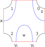
Figure 4.3. Heegaard diagram for the $(2,1)$-cabling operation. This is a doubly-pointed Heegaard diagram for the $(2,1)$ cable (of the unknot), thought of as a knot in the solid torus. The basepoint $z$ lies in the region marked with a $0$. This picture is adapted from [LOT08, Figure 11.14].

Example 4.10.

Figure 4.3 shows a doubly-pointed bordered Heegaard diagram inducing the $(2,1)$-cabling operation.

Given a doubly-pointed bordered Heegaard diagram $\mathcal{H}$, let $\mathit{CFD}^{-}(\mathcal{H},z,w)$ denote ${\mathbb{F}_{2}}[U]\otimes_{\mathbb{F}_{2}}\widehat{\mathit{CFD}}(\mathcal{H})$ with differential given by

$$\partial(\mathbf{x})=\sum_{\mathbf{y}\in\mathfrak{S}(\mathcal{H})}\sum_{n\geq 0}\sum_{(\rho_{1},\dots,\rho_{n})}\sum_{B\mid\operatorname{ind}(B,\rho_{1},\dots,\rho_{n})=1}\bigl{(}\#\mathcal{M}^{B}(\mathbf{x},\mathbf{y};\rho_{1},\dots,\rho_{n})\bigr{)}a(-\rho_{1})\cdots a(-\rho_{n})U^{n_{w}(B)}\mathbf{y}.$$

That is, we count curves as before except that we weight the curves which cross $w$ $n$ times by $U^{n}$.

Corollary 4.11.

With notation as above,

$$\mathit{gCFK}^{-}(L)\cong\operatorname{Mor}(\widehat{\mathit{CFD}}(-\mathcal{H}_{1}),\mathit{CFD}^{-}(\mathcal{H}_{2},z,w)).$$

By Theorem 4.6, $\widehat{\mathit{CFD}}(\mathcal{H}_{1})$ is determined by $\mathit{CFK}^{-}(K)$. Thus, if we can compute $\mathit{CFD}^{-}(\mathcal{H}_{2},z,w)$ we obtain a formula for the knot Floer complex $\mathit{gCFK}^{-}(L)$ in terms of $\mathit{CFK}^{-}(K)$ (for arbitrary $K$).

Example 4.12.

In [LOT08, Section 11.9] we use these techniques to compute the $(2,-3)$ cable of the left-handed trefoil. However, the computation there uses the type $A$ invariant of the pattern. In the spirit of continuing to avoid $\widehat{\mathit{CFA}}$, we give a similar computation using the $\operatorname{Mor}$ version of the pairing theorem.

Let $\mathcal{H}_{2}$ denote the doubly-pointed bordered Heegaard diagram shown in Figure 4.3. The module $\mathit{CFD}^{-}(\mathcal{H}_{2},z,w)$ has generators $x$, $y_{1}$ and $y_{2}$ with

$$\iota_{1}x =x \iota_{0}y_{1} =y_{1} \iota_{0}y_{2} =y_{2}.$$

The differentials are given by

$$\partial(x) =U^{2}\rho_{23}x$$

$$\partial(y_{1}) =Uy_{2}+\rho_{1}x$$

$$\partial(y_{2}) =U\rho_{123}x.$$

By Theorem 4.6, the invariant $\widehat{\mathit{CFD}}(Y)$ of the $2$-framed left-handed trefoil complement $Y$ is given by

$$\widehat{\mathit{CFD}}(Y)=\vbox{\hbox{$\leavevmode\hbox to112.68pt{\vbox to75.51pt{\text{[drawing]}}}$}} a \kappa b \lambda c. \rho_{1} \rho_{123} \rho_{3} \rho_{2} \rho_{12} a \kappa b \lambda c. \rho_{1} \rho_{123} \rho_{3} \rho_{2} \rho_{12}$$

As in Corollary 4.11, $\operatorname{Mor}(\widehat{\mathit{CFD}}(Y),\mathit{CFD}^{-}(\mathcal{H}_{2},z,w))$ is $\mathit{gCFK}^{-}$ of some cable of the left-handed trefoil. Computing this morphism space, a basis over ${\mathbb{F}_{2}}[U]$ is given by:

$$a \mapsto y_{1} a \mapsto\rho_{12}y_{1} a \mapsto y_{2} a \mapsto\rho_{12}y_{2}$$

$$a \mapsto\rho_{1}x a \mapsto\rho_{3}x a \mapsto\rho_{123}x$$

$$b \mapsto y_{1} b \mapsto\rho_{12}y_{1} b \mapsto y_{2} b \mapsto\rho_{12}y_{2}$$

$$b \mapsto\rho_{1}x b \mapsto\rho_{3}x b \mapsto\rho_{123}x$$

$$c \mapsto y_{1} c \mapsto\rho_{12}y_{1} c \mapsto y_{2} c \mapsto\rho_{12}y_{2}$$

$$c \mapsto\rho_{1}x c \mapsto\rho_{3}x c \mapsto\rho_{123}x$$

$$\lambda \mapsto x \lambda \mapsto\rho_{23}x \lambda \mapsto\rho_{2}y_{1} \lambda \mapsto\rho_{2}y_{2}$$

$$\kappa \mapsto x \kappa \mapsto\rho_{23}x \kappa \mapsto\rho_{2}y_{1} \kappa \mapsto\rho_{2}y_{2}.$$

(Nobody said this was quick. The complex is smaller if one uses $\widehat{\mathit{CFA}}(\mathcal{H}_{2},z,w)$.) The differentials are shown in Figure 4.4. Cancelling as many differentials not involving $U$ as possible gives Figure 4.5. In particular, the homology $\mathit{gHFK}^{-}(K)$ is given by ${\mathbb{F}_{2}}[U]\oplus\bigl{(}{\mathbb{F}_{2}}[U]/U^{2}\bigr{)}\oplus{\mathbb{F}_{2}}$; and $\widehat{\mathit{HFK}}(K)$ is given by $\mathbb{F}_{2}^{5}$.

Figure 4.4. The complex from Example 4.12

Figure 4.5. Result of cancelling differentials in Figure 4.4.

In some sense, this strategy works in general:

Lemma 4.13.

Given any pattern $P$ in $\mathbb{D}^{2}\times S^{1}$ there is a doubly-pointed Heegaard diagram inducing $P$.

The proof is left as Exercise 4.8.

Corollary 4.14.

Let $P$ be a knot in $\mathbb{D}^{2}\times S^{1}$. Given a knot $K$ in $S^{3}$ let $K^{P}$ denote the satellite of $K$ with pattern $P$. Then $\mathit{CFK}^{-}(K)$ determines $\mathit{gCFK}^{-}(K^{P})$ in the following sense: if $K_{1}$ and $K_{2}$ are knots with $\mathit{CFK}^{-}(K_{1})\cong\mathit{CFK}^{-}(K_{2})$ then $\mathit{gCFK}^{-}(K_{1}^{P})\cong\mathit{gCFK}^{-}(K_{2}^{P})$.

Remark 4.15.

The diagram $\mathcal{H}^{\prime}_{2}$ specifies more than just a knot in $\mathbb{D}^{2}\times S^{1}$; see Exercise 4.10. Probably the best way to think of $\mathcal{H}^{\prime}_{2}$ is as representing a bordered-sutured manifold (in the sense of [Zar09]).

4.4. Exercises

Exercise 4.1.

For $K$ the trefoil and the figure eight, compute the ${\mathbb{F}_{2}}[U]$ module structure on $H_{*}(\mathit{gCFK}^{-}(K))$, using the descriptions of the complexes given in Examples 4.3 and 4.4 respectively. Use this to compute $\tau(K)$ for these knots.

Exercise 4.2.

Find a basis for $\mathit{CFK}^{-}(K)$ when $K$ is the figure eight knot which is both horizontally and vertically simplified.

Exercise 4.3.

Let $Y$ be the complement of the unknot in $S^{3}$. Compute $\widehat{\mathit{CFD}}(Y)$ in two ways:

1. Using Theorem 4.6.

2. Directly from a bordered Heegaard diagram.

(This exercise is courtesy of J. Hom.)

Exercise 4.4.

Using Theorem 4.6, write down $\widehat{\mathit{CFD}}$ of the trefoil complement with framings $1$ and $-2$.

Exercise 4.5.

Figure 1.3 gives a bordered Heegaard diagram for the trefoil complement. Compute $\widehat{\mathit{CFD}}$ of that diagram directly, and compare the answer with that given by Theorem 4.6. (This is a fairly challenging computation, after which you are guaranteed to appreciated Theorem 4.6.)

Exercise 4.6.

Verify that the modules $\widehat{\mathit{CFD}}(Y)$ given by Theorem 4.6 satisfy $\partial^{2}=0$.

Exercise 4.7.

Prove Lemma 4.9.

Exercise 4.8.

Prove Lemma 4.13.

Exercise 4.9.

Use the bimodules of Exercise 2.6 to show that if Theorem 4.6 holds for surgery coefficient $n$ then it holds for surgery coefficient $n\pm 1$. (This is somewhat messy.)

Exercise 4.10.

Find doubly-pointed bordered Heegaard diagrams $\mathcal{H}$, $\mathcal{H}^{\prime}$ for $\mathbb{D}^{2}\times S^{1}$ so that:

• The singly-pointed Heegaard diagrams obtained from $\mathcal{H}$, $\mathcal{H}^{\prime}$ by forgetting the $w$ basepoint both specify the same framing for $\mathbb{D}^{2}\times S^{1}$.

• The diagrams $\mathcal{H}$ and $\mathcal{H}^{\prime}$ represent the same satellite operation in the sense of Construction 4.8.

• The invariants $\mathit{CFD}^{-}(\mathcal{H},z,w)$ and $\mathit{CFD}^{-}(\mathcal{H}^{\prime},z^{\prime},w^{\prime})$ are not homotopy equivalent.

In particular, it is not true that any two diagrams representing the same pattern $P$ are related by a sequence of Heegaard moves in the complement of the basepoints.

Exercise 4.11.

We computed $\mathit{gCFK}^{-}$ of some cable of the trefoil in Example 4.12. Which one?

Lecture 5 Computing with bordered Floer homology II: factoring mapping classes

The goal of this lecture is to discuss an algorithm, coming from bordered Floer homology, for computing the invariant $\widehat{\mathit{HF}}(Y)$ for any closed $3$-manifold $Y$. This is not the first algorithm for computing $\widehat{\mathit{HF}}(Y)$, which is due to Sarkar-Wang [SW10]; but it is independent of the Sarkar-Wang algorithm and conceptually fairly satisfying. The algorithm has been implemented using Sage; see http://math.columbia.edu/~lipshitz/research.html#Programming.

5.1. Overview of the algorithm

Fix a closed $3$-manifold $Y$ and a Heegaard splitting

$$Y=\mathsf{H}_{1}\cup_{\psi}\mathsf{H}_{2}$$

for $Y$. That is, $\mathsf{H}_{1}$ and $\mathsf{H}_{2}$ are handlebodies of some genus $k$ and $\psi\nobreak\mskip 2.0mu\mathpunct{}\nonscript\mkern-3.0mu{:}\penalty 300\mskip 6.0mu plus 1.0mu\partial\mathsf{H}_{1}\to\partial\mathsf{H}_{2}$ is an orientation-reversing homeomorphism.

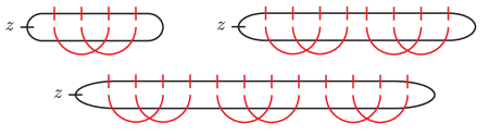
Figure 5.1. The pointed matched circles $\mathcal{Z}_{k}^{0}$. The cases $k=1$, $k=2$ and $k=3$ are shown.

Without loss of generality, we can assume that each $\mathsf{H}_{i}$ is a particular standard bordered handlebody $(\mathsf{H}_{k},\phi_{0}\nobreak\mskip 2.0mu\mathpunct{}\nonscript\mkern-3.0mu{:}\penalty 300\mskip 6.0mu plus 1.0muF(\mathcal{Z}_{k}^{0})\to\partial\mathsf{H}_{k})$. Here, $\mathcal{Z}_{k}^{0}$ is a particular pointed matched circle—we will take it to be the $k$-fold connect sum of the genus $1$ pointed matched circle (i.e., the split matching; see Figure 5.1). Then the map $\psi$ is specified by a map ${\widetilde{\psi}}=\phi_{0}\circ\psi\circ\phi_{0}^{-1}\nobreak\mskip 2.0mu\mathpunct{}\nonscript\mkern-3.0mu{:}\penalty 300\mskip 6.0mu plus 1.0muF(\mathcal{Z}_{k}^{0})\to F(\mathcal{Z}_{k}^{0})$. To specify $Y$ up to homeomorphism we need only specify $\psi$ up to isotopy; so, it is natural to view ${\widetilde{\psi}}$ as an element of the mapping class group of $F(\mathcal{Z}_{k}^{0})$. Up to isotopy, we can assume that ${\widetilde{\psi}}$ fixes the preferred disk in $F(\mathcal{Z}_{k}^{0})$, and regard it as an element of the mapping class group of $F^{\circ}(\mathcal{Z}_{k}^{0})$. (Of course, the lift to the strongly based mapping class group depends on a choice.)

Let $M_{{\widetilde{\psi}}}$ denote the mapping cylinder of ${\widetilde{\psi}}$, as in Example 1.13. Then by the relevant pairing theorems, Corollary 1.25 and Theorem 1.26, we have

$$\widehat{\mathit{CF}}(Y)\simeq\operatorname{Mor}\Bigl{(}\widehat{\mathit{CFD}}(\mathsf{H}_{k},\phi_{0}),\operatorname{Mor}\bigl{(}\widehat{\mathit{CFDD}}(-M_{\widetilde{\psi}}),\widehat{\mathit{CFD}}(\mathsf{H}_{k},\phi_{0})\bigr{)}\Bigr{)}.$$

So, we have “reduced” the problem to computing the invariants of $(\mathsf{H}_{k},\phi_{0})$ and $M_{\widetilde{\psi}}$.

This is not yet useful: there are about as many mapping classes as $3$-manifolds. On the other hand, the mapping classes form a group. Suppose that $\psi_{1},\dots,\psi_{N}$ are generators for the mapping class group of $F^{\circ}(\mathcal{Z}_{k}^{0})$ as a monoid—that is, we include inverses in our list of generators. Then we can write ${\widetilde{\psi}}=\psi_{i_{n}}\circ\dots\circ\psi_{i_{1}}$ for some sequence of generators $\psi_{i_{1}},\dots,\psi_{i_{n}}\in\{\psi_{1},\dots,\psi_{N}\}$. Repeatedly using Theorem 1.26, we have

$$\widehat{\mathit{CF}}(Y)\simeq\operatorname{Mor}\biggl{(}\widehat{\mathit{CFD}}(-\mathsf{H}_{k},\phi_{0}),\operatorname{Mor}\Bigl{(}\widehat{\mathit{CFDD}}(-M_{\psi_{i_{n}}}),\operatorname{Mor}\bigl{(}\cdots\\ \dots,\operatorname{Mor}(\widehat{\mathit{CFDD}}(-M_{\psi_{i_{1}}}),\widehat{\mathit{CFD}}(\mathsf{H}_{k},\phi_{0}))\dots\bigr{)}\Bigr{)}\biggr{)}.$$

So, we now really have reduced the problem: we only need to compute the invariants $\widehat{\mathit{CFD}}(\mathsf{H}_{k},\phi_{0})$ and $\widehat{\mathit{CFDD}}(M_{\psi_{i}})$ for our preferred set of generators $\psi_{1},\dots,\psi_{N}$.

5.1.1. Arc-slides as mapping class groupoid generators

Generalizing the mapping class group to a groupoid leads to a particularly convenient set of generators.

Definition 5.1.

The genus $k$ mapping class groupoid is the category whose objects are the pointed matched circles representing genus $g$ surfaces, and with $\operatorname{Hom}(\mathcal{Z}_{1},\mathcal{Z}_{2})$ the set of isotopy classes of strongly-based homeomorphisms $F(\mathcal{Z}_{1})\to F(\mathcal{Z}_{2})$.

In particular, $\operatorname{Aut}(\mathcal{Z})=\operatorname{Hom}(\mathcal{Z},\mathcal{Z})$ is the strongly-based mapping class group.

Figure 5.2. Arc-slides. Two examples of arc-slides connecting pointed matched circles for genus $2$ surfaces. In both cases, the foot $b_{1}$ is sliding over the matched pair $C=\{c_{1},c_{2}\}$ (indicated by the darker dotted matching) at $c_{1}$. This figure is [LOT10c, Figure LABEL:HFa:fig:ArcslideMatching].

Definition 5.2.

Let $\mathcal{Z}$ be a pointed matched circle, and fix two matched pairs $C=\{c_{1},c_{2}\}$ and $B=\{b_{1},b_{2}\}$ in $\mathcal{Z}$. Suppose moreover that $b_{1}$ and $c_{1}$ are adjacent, in the sense that there is an arc $\sigma$ connecting $b_{1}$ and $c_{1}$ which does not contain the basepoint $z$ or any other point $p_{i}\in\mathbf{a}$. Then we can form a new pointed matched circle $\mathcal{Z}^{\prime}$ which agrees everywhere with $\mathcal{Z}$, except that $b_{1}$ is replaced by a new distinguished point $b_{1}^{\prime}$, which now is adjacent to $c_{2}$ and $b_{1}^{\prime}$ is positioned so that the orientation on the arc from $b_{1}$ to $c_{1}$ is opposite to the orientation of the arc from $b_{1}^{\prime}$ to $c_{2}$. In this case, we say that $\mathcal{Z}^{\prime}$ and $\mathcal{Z}$ differ by an arc-slide of $b_{1}$ over $c_{1}$. (See Figure 5.2 for two examples.)

In this situation, there is a canonical element in $\operatorname{Hom}(\mathcal{Z},\mathcal{Z}^{\prime})$, which we refer to as the arc-slide diffeomorphism; see Figure 5.3.

Figure 5.3. The local case of an arc-slide diffeomorphism. Left: a pair of pants with boundary components labeled $P$, $Q$, and $R$, and two distinguished curves $B$ and $C$. Right: another pair of pants with boundary components $P^{\prime}$, $Q^{\prime}$, $R^{\prime}$ and distinguished curves $B^{\prime}$ and $C$. The arc-slide diffeomorphism carries $B$ to the dotted curve on the right, the curve labeled $C$ on the left to the curve labeled $C$ on the right, and boundary components $P$, $Q$, and $R$ to $P^{\prime}$, $Q^{\prime}$ and $R^{\prime}$ respectively. This diffeomorphism can be extended to a diffeomorphism between surfaces associated to pointed matched circles: in such a surface there are further handles attached along the four dark intervals; however, our diffeomorphism carries the four dark intervals on the left to the four dark intervals on the right and hence extends to a diffeomorphism as stated. (This is only one of several possible configurations of $B$ and $C$: they could also be nested or linked.) This figure is [LOT10c, Figure LABEL:HFa:fig:ArcSlide].

The diagrams in Figure 5.2 are shorthand for bordered Heegaard diagrams for the mapping cylinders of the arc-slides. Such a bordered Heegaard diagram for the second arc-slide in Figure 5.2 is given in Figure 5.4.

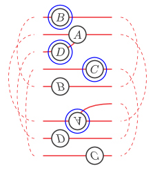
Figure 5.4. Heegaard diagram for an arc-slide. This diagram corresponds to the schematic on the right of Figure 5.2.

Lemma 5.3.

The arc-slides generate the mapping class groupoid.

A proof can be found in [Ben10]. It is perhaps a more familiar fact that the mapping class group is generated by some finite, preferred set of Dehn twists; see for example [Hum79]. Lemma 5.3 can be deduced from this more familiar fact by explicitly factoring that particular collection of Dehn twists into arcslides (see Example 5.4).

Example 5.4.

Figure 5.5 shows a factorization of a (particular) Dehn twist as a product of arc-slides.

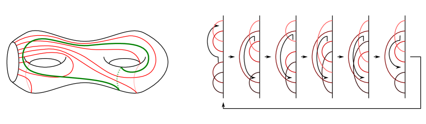
Figure 5.5. Factoring a Dehn twist into arc-slides. Left: a genus $2$ surface specified by a pointed matched circle, and a curve $\gamma$ (drawn in thick green) in it. Right: a sequence of arc-slides whose composition is a Dehn twist around $\gamma$. This is [LOT10c, Figure LABEL:HFa:fig:factor-Dehn].

So, two steps remain to compute $\widehat{\mathit{CF}}$:

• Compute $\widehat{\mathit{CFD}}(\mathcal{H}_{k})$ for some Heegaard diagram $\mathcal{H}_{k}$ representing the genus $k$ handlebody.

• Compute $\widehat{\mathit{CFDD}}(M_{\psi})$ for any arc-slide $\psi$.

We give these computations in Sections 5.2 and 5.4, respectively. (As a warm-up before computing the invariant of arc-slides we compute the type DD module associated to the identity cobordism.)

Remark 5.5.

The relations among arc-slides are also relatively easy to state; see [Ben10].

5.2. The invariant of a particular handlebody

Let $\mathcal{Z}^{1}$ denote the (unique) pointed matched circle for the torus, and let $\mathcal{Z}^{k}$ denote the $k$-fold connect sum of $\mathcal{Z}^{1}$ with itself, i.e., the genus $k$ split pointed matched circle. Label the marked points in $\mathcal{Z}^{k}$ as $a_{1},\dots,a_{4k}$. So, in $\mathcal{Z}^{k}$ the matched pairs are $\{a_{4i-3},a_{4i-1}\}$ and $\{a_{4i},a_{4i-2}\}$.

The $0$-framed solid torus $\mathsf{H}^{1}=(H^{1},\phi^{1}_{0})$ is the solid torus with boundary $-{F(\mathcal{Z}^{1})}$ in which the handle determined by $\{a_{1},a_{3}\}$ bounds a disk. Let $\phi^{1}_{0}$ denote the preferred diffeomorphism $-{F(\mathcal{Z}^{1})}\to\partial H^{1}$. The $0$-framed handlebody of genus $k$ $\mathsf{H}^{k}=(H^{k},\phi^{k}_{0})$ is a boundary connect sum of $k$ copies of $\mathsf{H}^{1}$. Our conventions are illustrated by the bordered Heegaard diagram in Figure 5.6.

Figure 5.6. Heegaard diagram for the $0$-framed genus two handlebody. The lighter (respectively darker) shaded pair of circles indicates a handle attached to the diagram. This is [LOT10c, Figure LABEL:HFa:fig:GenusTwoBorderedDiagram].

Proposition 5.6.

Let $\mathbf{s}=\{a_{4i-3},a_{4i-1}\}_{i=1}^{k}$. The module $\widehat{\mathit{CFD}}(\mathsf{H}^{k})$ is generated over the algebra by a single element $\mathbf{x}$ with $I(\mathbf{s})\mathbf{x}=\mathbf{x}$, and is equipped with the differential determined by

$$\partial(\mathbf{x})=\sum_{i=1}^{k}a(\xi_{i})\mathbf{x},$$

where $\xi_{i}$ is the arc in $\mathcal{Z}^{k}$ connecting $a_{4i-3}$ and $a_{4i-1}$.

Proof.

This is a simple computation from the definitions. Note that the domains of holomorphic curves contributing to the differential on $\widehat{\mathit{CFD}}(\mathsf{H}^{k})$ must be connected. It follows that the curves appearing here are simply copies of the curves occurring in the differential on $\widehat{\mathit{CFD}}(\mathsf{H}^{1})$. These, in turn, were already studied in Section 2.4. ∎

5.3. The DD identity

Let $\mathbb{I}$ denote the identity arced cobordism of $F(\mathcal{Z})$. As a warm-up to computing the bimodules associated to arc-slides we compute the bimodule $\widehat{\mathit{CFDD}}(\mathbb{I})$. The standard bordered Heegaard diagram $\mathcal{H}(\mathbb{I})$ for the identity cobordism (for a particular choice of $\mathcal{Z}$) is illustrated in Figure 5.7. Inspecting the diagram, one has two immediate observations:

1. Recall that indecomposable idempotents of $\mathcal{A}(\mathcal{Z})$ correspond to subsets of the matched pairs in $\mathcal{Z}$. There is an obvious bijection between matched pairs in $\mathcal{Z}$ and matched pairs in $-\mathcal{Z}$. With respect to this bijection, the generators of $\widehat{\mathit{CFDD}}(\mathbb{I})$ correspond one-to-one with pairs of indecomposable idempotents $I(\mathbf{s})\otimes I(\mathbf{t})\in\mathcal{A}(\mathcal{Z})\otimes\mathcal{A}(-\mathcal{Z})$ with $\mathbf{s}\cap\mathbf{t}=\emptyset$. We call such pairs complementary idempotents. (The set of complementary idempotents is also in bijection with the set of idempotents of $\mathcal{A}(\mathcal{Z})$, of course.)

   Given a pair of complementary idempotents $I\otimes I^{\prime}$ let $\mathbf{x}_{I,I^{\prime}}$ denote the corresponding generator of $\widehat{\mathit{CFDD}}(\mathbb{I})$.

2. Any domain in $\mathcal{H}(\mathbb{I})$ has the same multiplicities at the two boundaries of $\mathcal{H}(\mathbb{I})$. Any basic element of $\mathcal{A}(\mathcal{Z})$ has an associated support in $H_{1}(Z\setminus\{z\},{\mathbf{a}})$; let $[\xi]$ denote the support of $\xi$. It follows that if $(\xi\otimes\xi^{\prime})\otimes\mathbf{x}_{J,J^{\prime}}$ occurs in $\partial(\mathbf{x}_{I,I^{\prime}})$ then $[\xi]=[\xi^{\prime}]$ (in the obvious sense).

Figure 5.7. Heegaard diagram for the identity map. This is a Heegaard diagram for the identity cobordism of the genus two surface with antipodal matching, as indicated by the arcs to the left of the diagram. To the left and the right of the diagram, we have also indicated a pair of complementary idempotents, along with its unique extension into the diagram as a generator for the complex. This figure is [LOT10c, Figure LABEL:HFa:fig:Genus2Identity].

Formalizing the above, let the diagonal subalgebra of $\mathcal{A}(\mathcal{Z})\otimes\mathcal{A}(-\mathcal{Z})$ denote the subalgebra with basis

$$\{(I\cdot\xi\cdot J)\otimes(I^{\prime}\cdot\xi^{\prime}\cdot J^{\prime})\mid[\xi]=[\xi^{\prime}],\ (I,I^{\prime})\text{ complementary},\ (J,J^{\prime})\text{ complementary}\}.$$

Proposition 5.7.

The diagonal subalgebra has a $\mathbb{Z}$-grading $\operatorname{gr}$ with the following properties:

1. The grading $\operatorname{gr}$ respects the differential algebra structure, i.e., for homogeneous elements $a$ and $b$, $\operatorname{gr}(ab)=\operatorname{gr}(a)+\operatorname{gr}(b)$ and $\operatorname{gr}(d(a))=\operatorname{gr}(a)-1$.

2. The differential on $\widehat{\mathit{CFDD}}(\mathbb{I})$ is homogeneous of degree $-1$ with respect to $\operatorname{gr}$.

3. The standard basis elements for the diagonal subalgebra are homogeneous with respect to $\operatorname{gr}$.

4. If $a\in\mathcal{A}$ is homogeneous then $\operatorname{gr}(a)\leq 0$.

5. If $\operatorname{gr}(a)=0$ then $a$ is an idempotent.

6. If $\operatorname{gr}(a)=-1$ then $a$ is a linear combination of chords, i.e., elements of the form $a(\rho)\otimes a^{\prime}(\rho)$ where $\rho$ is a single chord in $\mathcal{Z}$. (Here, $a^{\prime}(\rho)$ denotes the element of $\mathcal{A}(-\mathcal{Z})$ associated to the chord $\rho$.)

Sketch of proof..

There are at least two ways to go about this proof. One is to show that any element of the diagonal algebra can be factored as a product of chords, and the length of the factorization is unique. (This is the approach taken in [LOT10c, Section LABEL:HFa:sec:DDforIdentity].) Another approach is to observe that there is a dg algebra with properties (1) and (2) associated to any type DD bimodule (or type $D$ module); we call this the coefficient algebra [LOT10c, Sections LABEL:HFa:sec:coeff-algebra and LABEL:HFa:sec:coeff-bimod]. In the case of $\widehat{\mathit{CFDD}}(\mathbb{I})$, the coefficient algebra is exactly the diagonal subalgebra. Verifying the remaining properties above is then a fairly simple computation. (This is the approach taken for arc-slide bimodules in [LOT10c, Section LABEL:HFa:sec:Arc-Slides].) ∎

Corollary 5.8.

If $(a\otimes b)\otimes\mathbf{x}_{J,J^{\prime}}$ occurs in $\partial(\mathbf{x}_{I,I^{\prime}})$ then $a\otimes b$ is a linear combination of chords $a(\rho_{i})\otimes a(\rho^{\prime}_{i})$.

Let $\mathrm{Chord}(\mathcal{Z})$ denote the set of all chords for $\mathcal{Z}$.

Theorem 5.9.

As a bimodule, $\widehat{\mathit{CFDD}}(\mathbb{I})$ is given by

$$\widehat{\mathit{CFDD}}(\mathbb{I})=\bigoplus_{(I\otimes I^{\prime})\text{ complementary}}(\mathcal{A}(\mathcal{Z})\cdot I)\otimes_{\mathbb{F}_{2}}(\mathcal{A}(-\mathcal{Z})\cdot I^{\prime})\otimes\mathbf{x}_{I,I^{\prime}}.$$

The differential of $\mathbf{x}_{I,I^{\prime}}$ is given by

$$\partial(\mathbf{x}_{I,I^{\prime}})=\sum_{(J,J^{\prime})}\sum_{\rho\in\mathrm{Chord}(\mathcal{Z})}\bigl{[}(I\cdot a(\rho)\cdot J)\otimes(I^{\prime}\cdot a^{\prime}(\rho)\cdot J^{\prime})\bigr{]}\otimes\mathbf{x}_{J,J^{\prime}}.$$

In other word, every term permitted by Corollary 5.8 to occur in $\partial(\mathbf{x}_{I,I^{\prime}})$ does occur.

Sketch of proof.

All that remains is to show that every term of the form $\bigl{[}(I\cdot a(\rho)\cdot J)\otimes(I^{\prime}\cdot a^{\prime}(\rho)\cdot J^{\prime})\bigr{]}\otimes\mathbf{x}_{J,J^{\prime}}$ does occur in $\partial\mathbf{x}_{I,I^{\prime}}$. The argument is by induction on the support to $\rho$. The base case is when $\rho$ has length $1$. In this case, the corresponding domain in $\mathcal{H}(\mathbb{I})$ is a hexagon, so it follows from the Riemann mapping theorem that there is a holomorphic representative.

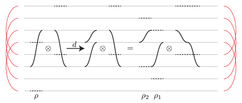
Figure 5.8. Illustration of the inductive step in the proof of Theorem 5.9. We want to show the term on the left occurs in $\partial$ on $\widehat{\mathit{CFDD}}(\mathbb{I})$. The term on the far right occurs in $\partial^{2}$, by induction on the length of the chords involved. The only other contribution to $\partial^{2}$ which could cancel it is the differential of the term on the left. (The differential of the term on the left also has other terms, not shown.)

The rest of the induction argument is illustrated in Figure 5.8. In words, suppose $\rho$ has length bigger than $1$, and suppose there is a position $a\in{\mathbf{a}}$ so that:

• $a$ lies in the interior of $\rho$ and

• the matched pair containing $a$ is in the idempotent $I$.

Let $\rho_{1}$ be the chord from the start of $\rho$ to the point $a$ and let $\rho_{2}$ be the chord from $a$ to the end of $\rho$. By induction, $\partial^{2}(\mathbf{x}_{I,I^{\prime}})$ contains a term of the form $\bigl{[}(I\cdot a(\rho_{2})a(\rho_{1})J)\otimes(I^{\prime}\cdot a^{\prime}(\rho)\cdot J^{\prime})\bigr{]}\otimes\mathbf{x}_{J,J^{\prime}}$; this term comes from the sequence

$$\mathbf{x}_{I,I^{\prime}} \stackrel{{\scriptstyle\partial}}{{\longrightarrow}}\bigl{[}(I\cdot a(\rho_{2}))\otimes(I^{\prime}\cdot a^{\prime}(\rho_{2}))\bigr{]}\otimes\mathbf{x}_{K,K^{\prime}}$$

$$\stackrel{{\scriptstyle\partial}}{{\longrightarrow}}\bigl{[}(I\cdot a(\rho_{2})a(\rho_{1}))\otimes(I^{\prime}\cdot a^{\prime}(\rho_{2})a^{\prime}(\rho_{1}))\bigr{]}\otimes\mathbf{x}_{J,J^{\prime}}$$

$$\qquad\qquad\qquad=\bigl{[}(I\cdot a(\rho_{2})a(\rho_{1}))\otimes(I^{\prime}\cdot a^{\prime}(\rho))\bigr{]}\otimes\mathbf{x}_{J,J^{\prime}}.$$

The only term in $\partial^{2}(\mathbf{x}_{I,I^{\prime}})$ which could cancel this one is $\bigl{[}(I\cdot\partial a(\rho)\cdot J)\otimes(I\cdot a^{\prime}(\rho)\cdot J^{\prime})\bigr{]}\otimes\mathbf{x}_{J,J^{\prime}}$. Thus, since $\partial^{2}=0$, the term $\bigl{[}(I\cdot a(\rho)\cdot J)\otimes(I\cdot a^{\prime}(\rho)\cdot J^{\prime})\bigr{]}\otimes\mathbf{x}_{J,J^{\prime}}$ must occur in $\partial(\mathbf{x}_{I,I^{\prime}})$.

If there is a position $a$ in the interior of $\rho$ occupied in the idempotent $I^{\prime}$ then a similar argument, with the left and right sides reversed, gives the result. The only other case is that of length three chords in which both of the interior positions are matched to the endpoints. We call such chords special length $3$ chords in [LOT10c]. There are various ways to handle this case. A somewhat indirect argument is given in the proof of [LOT10c, Theorem LABEL:HFa:thm:DDforIdentity]. One can also prove the result in this case by a direct computation, as in the proof of [LOT10a, Proposition LABEL:LOT2:prop:TypeDDTorus]. ∎

Remark 5.10.

The bimodule $\widehat{\mathit{CFDD}}(\mathbb{I})$ exhibits a kind of duality between the algebras $\mathcal{A}(\mathcal{Z})$ and $\mathcal{A}(-\mathcal{Z})$, called Koszul duality. See, for instance, [LOT11a, Section LABEL:HomPair:sec:koszul].

5.4. Underslides

To explain the bimodule $\widehat{\mathit{CFDD}}$ associated to an arc-slide we first divide the arc-slides into two classes: underslides and overslides. Specifically, with notation as in Definition 5.2, $Z\setminus C$ has two connected components. One of these components contains the basepoint $z$; call that component $Z_{z}$. Then an arc-slide is an overslide if $b_{1}\in Z_{z}$, and is an underslide if $b_{1}\not\in Z_{z}$. So, in Figure 5.2, the example on the left is an overslide while the example on the right is an underslide.

It turns out that the bimodules for underslides are a little simpler, so we will focus on this case, referring the reader to [LOT10c, Section LABEL:HFa:subsec:Over-Slides] for the overslide case. So, let $\psi\nobreak\mskip 2.0mu\mathpunct{}\nonscript\mkern-3.0mu{:}\penalty 300\mskip 6.0mu plus 1.0mu\mathcal{Z}\to\mathcal{Z}^{\prime}$ be an underslide and $M_{\psi}$ the associated mapping cylinder. To describe $\widehat{\mathit{CFDD}}(M_{\psi})$ we need two more pieces of terminology:

Definition 5.11.

There is an obvious bijection between matched pairs of $\mathcal{Z}$ (i.e., $1$-handles of $F(\mathcal{Z})$) and matched pairs of $\mathcal{Z}^{\prime}$ (i.e., $1$-handles of $F(\mathcal{Z})$). With notation as in Definition 5.2, a pair of indecomposable idempotents $I(\mathbf{s})\otimes I(\mathbf{s}^{\prime})\in\mathcal{A}(\mathcal{Z})\otimes\mathcal{A}(-\mathcal{Z}^{\prime})$ are called near-complementary if either:

• $\mathbf{s}$ is complementary to $\mathbf{s}^{\prime}$ or

• $\mathbf{s}\cap\mathbf{t}$ consists of the matched pair of the feet of $C$, while $\mathbf{s}\cup\mathbf{t}$ contains all the matched pairs except for the pair of feet of $B$.

Figure 5.9. Near-chords for under-slides.

Definition 5.12.

A near-chord for the underslide $\psi$ is an algebra element of the form $a(\xi)\otimes a^{\prime}(\xi^{\prime})$ where $\xi$ (respectively $\xi^{\prime}$) is a collection of chords in $\mathcal{Z}$ (respectively $-\mathcal{Z}^{\prime}$) of one of the forms (U-1)–(U-6) shown in Figure 5.9.

Let $\mathrm{NChord}(\psi)$ denote the set of near-chords for $\psi$.

(See [LOT10c, Definition LABEL:HFa:def:UnderNearChord] for a more detailed description of the types (U-1)–(U-6) of near-chords.)

Theorem 5.13.

The bimodule $\widehat{\mathit{CFDD}}(M_{\psi})$ has one generator $\mathbf{x}_{I,I^{\prime}}$ for each near-complementary pair of idempotents $I\otimes I^{\prime}$; and $\mathbf{x}_{I,I^{\prime}}=(I\otimes I^{\prime})\cdot\mathbf{x}_{I,I^{\prime}}$. (In other words, as a module $\widehat{\mathit{CFDD}}(M_{\psi})\cong\bigoplus_{I\otimes I^{\prime}\text{ near complementary}}\bigl{(}\mathcal{A}(\mathcal{Z})\cdot I\bigr{)}\otimes\bigl{(}\mathcal{A}(-\mathcal{Z}^{\prime})\cdot I^{\prime}\bigr{)}.$) The differential on $\widehat{\mathit{CFDD}}(M_{\psi})$ is given by

$$\partial(\mathbf{x}_{I,I^{\prime}})=\sum_{\begin{subarray}{c}(J,J^{\prime})\\ \text{ near-complementary}\end{subarray}}\sum_{(\xi,\xi^{\prime})\in\mathrm{NChord}(\psi)}\bigl{[}(I\cdot a(\xi)\cdot J)\otimes(I^{\prime}\cdot a^{\prime}(\xi^{\prime})\cdot J^{\prime})\bigr{]}\otimes\mathbf{x}_{J,J^{\prime}}.$$

Sketch of proof..

The proof is similar to, though more involved than, the proof of Theorem 5.9. There is an analogue of the diagonal algebra, called the near-diagonal algebra, admitting a $\mathbb{Z}$-grading satisfying analogous properties to Proposition 5.7. In particular, the near-chords are exactly the basic elements in grading $-1$. So, it only remains to show that every near-chord occurs in the differential. This follows from an inductive argument similar to the proof of Theorem 5.9. For short near-chords—near chords of type (U-2) and minimal-length near-chords of types (U-1) and (U-4)—it follows from the Riemann mapping theorem that the chords occur in the differential. The existence of other near-chords follows by a (somewhat complicated) induction on the support, using only the fact that $\partial^{2}=0$. ∎

We do not discuss the case of overslides, which are more complicated than underslides. At the heart of the complication is the fact that, for overslides, the coefficient algebra contains non-idempotent elements in grading $0$ (whereas in the underslide case, all non-idempotent elements have negative grading). While in the underslide case, every element in grading $-1$ appears as a coefficient in the differential, in the overslide case which grading $-1$ elements appear depends on a choice. Nonetheless, the index zero elements can be used to induce maps between bimodules associated to the various choices, and a somewhat weaker analogue of Theorem 5.13 holds: the overslide bimodule can be computed explicitly after some combinatorial choices are made, and the homotopy type of the answer is independent of those combinatorial choices. The interested reader is referred to [LOT11a, Proposition LABEL:HFa:prop:CalculateOver-Slide].

5.5. Exercises

Exercise 5.1.

Verify the type DD bimodule for the identity cobordism of the torus given in Exercise 2.4 agrees with the answer given by Theorem 5.9.

Exercise 5.2.

Verify that the bimodules from Exercise 2.6 agree with the bimodules given by Theorem 5.13. (Note that one can view each of these Dehn twists as an underslide.)

Exercise 5.3.

Extend the algorithm above to compute $\widehat{\mathit{CFD}}(Y)$ for any bordered $3$-manifold $Y$.

Bibliography

- [Aur10] Denis Auroux, Fukaya categories of symmetric products and bordered Heegaard-Floer homology, J. Gökova Geom. Topol. 4 (2010), 1–54, arXiv:1001.4323.
- [BEH+03] Frédéric Bourgeois, Yakov Eliashberg, Helmut Hofer, Kris Wysocki, and Eduard Zehnder, Compactness results in symplectic field theory, Geom. Topol. 7 (2003), 799–888, arXiv:math.SG/0308183.
- [Ben10] Alex James Bene, A chord diagrammatic presentation of the mapping class group of a once bordered surface, Geom. Dedicata 144 (2010), 171–190, arXiv:0802.2747.
- [BG12] John A. Baldwin and William D. Gillam, Computations of Heegaard-Floer knot homology, J. Knot Theory Ramifications 21 (2012), no. 8, 1250075, arXiv:math/0610167.
- [BL94] Joseph Bernstein and Valery Lunts, Equivariant sheaves and functors, Lecture Notes in Mathematics, vol. 1578, Springer-Verlag, Berlin, 1994.
- [CGH12a] Vincent Colin, Paolo Ghiggini, and Ko Honda, The equivalence of Heegaard Floer homology and embedded contact homology via open book decompositions I, 2012, arXiv:1208.1074.
- [CGH12b] by same author, The equivalence of Heegaard Floer homology and embedded contact homology via open book decompositions II, 2012, arXiv:1208.1077.
- [CGH12c] by same author, The equivalence of Heegaard Floer homology and embedded contact homology III: from hat to plus, 2012, arXiv:1208.1526.
- [Ghi08] Paolo Ghiggini, Knot Floer homology detects genus-one fibred knots, Amer. J. Math. 130 (2008), no. 5, 1151–1169.
- [GMM05] Hiroshi Goda, Hiroshi Matsuda, and Takayuki Morifuji, Knot Floer homology of -knots, Geom. Dedicata 112 (2005), 197–214.
- [Hed05] Matthew Hedden, On knot Floer homology and cabling, Algebr. Geom. Topol. 5 (2005), 1197–1222, arXiv:math.GT/0406402.
- [Hom12] Jennifer Hom, Bordered Heegaard Floer homology and the tau-invariant of cable knots, 2012, arXiv:1202.1463.
- [Hum79] Stephen P. Humphries, Generators for the mapping class group, Topology of low-dimensional manifolds (Proc. Second Sussex Conf., Chelwood Gate, 1977), Lecture Notes in Math., vol. 722, Springer, Berlin, 1979, pp. 44–47.
- [JM08] Stanislav Jabuka and Thomas E. Mark, Product formulae for Ozsváth-Szabó 4-manifold invariants, Geom. Topol. 12 (2008), no. 3, 1557–1651.
- [JT12] András Juhász and Dylan P. Thurston, Naturality and mapping class groups in Heegaard Floer homology, 2012, arXiv:1210.4996.
- [Juh06] András Juhász, Holomorphic discs and sutured manifolds, Algebr. Geom. Topol. 6 (2006), 1429–1457, arXiv:math/0601443.
- [Kho01] Mikhail Khovanov, Nilcoxeter algebras categorify the Weyl algebra, Comm. Algebra 29 (2001), no. 11, 5033–5052, arXiv:math.RT/9906166.
- [Kho10] by same author, How to categorify one-half of quantum , 2010, arXiv:1007.3517.
- [KLT10a] Çağatay Kutluhan, Yi-Jen Lee, and Clifford Henry Taubes, HF=HM I: Heegaard Floer homology and Seiberg–Witten Floer homology, 2010, arXiv:1007.1979.
- [KLT10b] by same author, HF=HM II: Reeb orbits and holomorphic curves for the ech/Heegaard-Floer correspondence, 2010, 1008.1595.
- [KLT10c] by same author, HF=HM III: Holomorphic curves and the differential for the ech/Heegaard Floer correspondence, 2010, arXiv:1010.3456.
- [KLT11] by same author, HF=HM IV: The Seiberg-Witten Floer homology and ech correspondence, 2011, arXiv:1107.2297.
- [KLT12] by same author, HF=HM V: Seiberg-Witten Floer homology and handle additions, 2012, arXiv:1204.0115.
- [Lev12a] Adam Simon Levine, Knot doubling operators and bordered Heegaard Floer homology, J. Topol. 5 (2012), no. 3, 651–712, arXiv:1008.3349.
- [Lev12b] by same author, Slicing mixed Bing-Whitehead doubles, J. Topol. 5 (2012), no. 3, 713–726, arXiv:0912.5222.
- [Lip06] Robert Lipshitz, A cylindrical reformulation of Heegaard Floer homology, Geom. Topol. 10 (2006), 955–1097, arXiv:math.SG/0502404.
- [LOTa] Robert Lipshitz, Peter S. Ozsváth, and Dylan P. Thurston, Bordered Floer homology and the spectral sequence of a branched double cover II: the spectral sequences agree, in preparation.
- [LOTb] by same author, Computing cobordism maps with bordered Floer homology, in preparation.
- [LOT08] by same author, Bordered Heegaard Floer homology: Invariance and pairing, 2008, arXiv:0810.0687v4.
- [LOT09] by same author, Slicing planar grid diagrams: a gentle introduction to bordered Heegaard Floer homology, Proceedings of Gökova Geometry-Topology Conference 2008, Gökova Geometry/Topology Conference (GGT), Gökova, 2009, pp. 91–119, arXiv:0810.0695.
- [LOT10a] by same author, Bimodules in bordered Heegaard Floer homology, 2010, arXiv:1003.0598v3.
- [LOT10b] by same author, Bordered Floer homology and the spectral sequence of a branched double cover I, 2010, arXiv:1011.0499.
- [LOT10c] by same author, Computing by factoring mapping classes, 2010, arXiv:1010.2550v3.
- [LOT11a] Robert Lipshitz, Peter S. Ozsváth, and Dylan P. Thurston, Heegaard Floer homology as morphism spaces, Quantum Topology 2 (2011), no. 4, 384–449, arXiv:1005.1248.
- [LOT11b] Robert Lipshitz, Peter S. Ozsváth, and Dylan P. Thurston, Tour of bordered Floer theory, Proc. Natl. Acad. Sci. USA 108 (2011), no. 20, 8085–8092, arXiv:1107.5621.
- [LOT13] by same author, A faithful linear-categorical action of the mapping class group of a surface with boundary, J. Eur. Math. Soc. (JEMS) 15 (2013), no. 4, 1279–1307, arXiv:1012.1032.
- [MO10] Ciprian Manolescu and Peter Ozsváth, Heegaard Floer homology and integer surgeries on links, 2010, arXiv:1011.1317.
- [MOS09] Ciprian Manolescu, Peter Ozsváth, and Sucharit Sarkar, A combinatorial description of knot Floer homology, Ann. of Math. (2) 169 (2009), no. 2, 633–660, arXiv:math.GT/0607691.
- [MOSzT07] Ciprian Manolescu, Peter S. Ozsváth, Zoltán Szabó, and Dylan P. Thurston, On combinatorial link Floer homology, Geom. Topol. 11 (2007), 2339–2412, arXiv:math.GT/0610559.
- [MOT09] Ciprian Manolescu, Peter Ozsváth, and Dylan Thurston, Grid diagrams and Heegaard Floer invariants, 2009, arXiv:0910.0078.
- [Ni09] Yi Ni, Heegaard Floer homology and fibred 3-manifolds, Amer. J. Math. 131 (2009), no. 4, 1047–1063.
- [OSSz09] Peter Ozsváth, András Stipsicz, and Zoltán Szabó, Floer homology and singular knots, J. Topol. 2 (2009), no. 2, 380–404.
- [OSz03] Peter S. Ozsváth and Zoltán Szabó, Heegaard Floer homology and alternating knots, Geom. Topol. 7 (2003), 225–254 (electronic).
- [OSz04a] by same author, Holomorphic disks and genus bounds, Geom. Topol. 8 (2004), 311–334.
- [OSz04b] by same author, Holomorphic disks and knot invariants, Adv. Math. 186 (2004), no. 1, 58–116, arXiv:math.GT/0209056.
- [OSz04c] by same author, Holomorphic disks and three-manifold invariants: properties and applications, Ann. of Math. (2) 159 (2004), no. 3, 1159–1245, arXiv:math.SG/0105202.
- [OSz04d] by same author, Holomorphic disks and topological invariants for closed three-manifolds, Ann. of Math. (2) 159 (2004), no. 3, 1027–1158, arXiv:math.SG/0101206.
- [OSz04e] by same author, Holomorphic triangle invariants and the topology of symplectic four-manifolds, Duke Math. J. 121 (2004), no. 1, 1–34.
- [OSz05a] by same author, On knot Floer homology and lens space surgeries, Topology 44 (2005), no. 6, 1281–1300, arXiv:math/0303017.
- [OSz05b] by same author, On the Heegaard Floer homology of branched double-covers, Adv. Math. 194 (2005), no. 1, 1–33, arXiv:math.GT/0309170.
- [OSz06] by same author, Holomorphic triangles and invariants for smooth four-manifolds, Adv. Math. 202 (2006), no. 2, 326–400, arXiv:math.SG/0110169.
- [OSz08] by same author, Knot Floer homology and integer surgeries, Algebr. Geom. Topol. 8 (2008), no. 1, 101–153.
- [OSz09] Peter Ozsváth and Zoltán Szabó, A cube of resolutions for knot Floer homology, J. Topol. 2 (2009), no. 4, 865–910.
- [Per08] Timothy Perutz, Hamiltonian handleslides for Heegaard Floer homology, Proceedings of Gökova Geometry-Topology Conference 2007, Gökova Geometry/Topology Conference (GGT), Gökova, 2008, pp. 15–35.
- [Pet09] Ina Petkova, Cables of thin knots and bordered Heegaard Floer homology, 2009, arXiv:0911.2679.
- [Ras03] Jacob Rasmussen, Floer homology and knot complements, Ph.D. thesis, Harvard University, Cambridge, MA, 2003, arXiv:math.GT/0306378.
- [Rob08] Lawrence P. Roberts, Rational blow-downs in Heegaard-Floer homology, Commun. Contemp. Math. 10 (2008), no. 4, 491–522.
- [SW10] Sucharit Sarkar and Jiajun Wang, An algorithm for computing some Heegaard Floer homologies, Ann. of Math. (2) 171 (2010), no. 2, 1213–1236, arXiv:math/0607777.
- [Tau10a] Clifford Henry Taubes, Embedded contact homology and Seiberg-Witten Floer cohomology I, Geom. Topol. 14 (2010), no. 5, 2497–2581.
- [Tau10b] by same author, Embedded contact homology and Seiberg-Witten Floer cohomology II, Geom. Topol. 14 (2010), no. 5, 2583–2720.
- [Tau10c] by same author, Embedded contact homology and Seiberg-Witten Floer cohomology III, Geom. Topol. 14 (2010), no. 5, 2721–2817.
- [Tau10d] by same author, Embedded contact homology and Seiberg-Witten Floer cohomology IV, Geom. Topol. 14 (2010), no. 5, 2819–2960.
- [Tau10e] by same author, Embedded contact homology and Seiberg-Witten Floer cohomology V, Geom. Topol. 14 (2010), no. 5, 2961–3000.
- [Zar09] Rumen Zarev, Bordered Floer homology for sutured manifolds, 2009, arXiv:0908.1106.