Cooperative Sparsity Pattern Recovery in Distributed Networks Via Distributed-OMP

Abstract

In this paper, we consider the problem of collaboratively estimating the sparsity pattern of a sparse signal with multiple measurement data in distributed networks. We assume that each node makes Compressive Sensing (CS) based measurements via random projections regarding the same sparse signal. We propose a distributed greedy algorithm based on Orthogonal Matching Pursuit (OMP), in which the sparse support is estimated iteratively while fusing indices estimated at distributed nodes. In the proposed distributed framework, each node has to perform less number of iterations of OMP compared to the sparsity index of the sparse signal. Thus, with each node having a very small number of compressive measurements, a significant performance gain in support recovery is achieved via the proposed collaborative scheme compared to the case where each node estimates the sparsity pattern independently and then fusion is performed to get a global estimate. We further extend the algorithm to estimate the sparsity pattern in a binary hypothesis testing framework, where the algorithm first detects the presence of a sparse signal collaborating among nodes with a fewer number of iterations of OMP and then increases the number of iterations to estimate the sparsity pattern only if the signal is detected.

Keywords: Compressive sensing, Sparsity pattern recovery, multiple measurement vectors, distributed networks

I Introduction

In the Compressive Sensing (CS) framework, a small collection of linear random projections of a sparse signal contains sufficient information for complete signal recovery [1, 2, 3]. There is a considerable amount of work on the development of computationally efficient and tractable algorithms to recover sparse signals from CS based measurements obtained via random projections, for example in [4, 5, 6, 7, 8, 9, 10, 11, 12]. However, there are several signal processing applications where complete signal recovery is not necessary. For example, in applications such as source localization in sensor networks [13, 14], estimation of frequency band locations in cognitive radio networks [15], localization of neural electrical activities from a huge number of potential locations in magnetoencephalography (MEG) and electroencephalography (EEG) for medical imaging applications [16, 17, 18], sparse approximation [19], subset selection in linear regression [20, 21], and signal denoising [22], it is only necessary to estimate the locations of the significant coefficients of a sparse signal.

I-A Related work and our contribution

The problem of sparsity pattern estimation of sparse signals has been addressed by several authors in the literature in the context of CS [23, 24, 25, 26, 27, 28, 29, 30, 31]. These studies focus on CS based sparsity pattern recovery with a single measurement vector. The achievable performance can be improved by having multiple observation vectors. Further, in distributed networks including sensor networks and cooperative cognitive radio networks, multiple measurements appear quite naturally since multiple nodes make observations regarding the same phenomenon of interest (PoI). Extensions of sparse signal recovery with multiple measurement vectors are considered in [32, 33] assuming that the multiple measurements are available at a single location to perform the desired task. In such centralized settings, each node in the network has to transmit its observations along with the elements of the measurement matrix to solve the sparse signal recovery problem at the central fusion center. However, when performing inference tasks based on the observations collected at different nodes in distributed networks, the trade-off between the resource constraints (e.g. node power and communication bandwidth) and the achievable performance gain is a core issue to be addressed in many practical networks. Thus, distributed approaches for sparsity pattern recovery are desirable in many practical distributed networks where each node has limited computational and communication power/bandwidth. The problem of distributed sparsity pattern recovery is considered recently in the context of cognitive radio networks in [34, 35]. There, decentralized consensus based algorithms for support recovery of sparse signals were proposed when each cognitive radio makes CS based measurements in cooperative cognitive radio networks.

The work in this paper focuses on further reducing the computational and communication burden at individual nodes in a distributed network while performing sparsity pattern recovery when each node in the network observes a noisy version of the same sparse signal. In contrast to transmitting raw observations along with measurement matrices to a central fusion center to perform centralized sparsity pattern recovery, we consider the case where each node tries to find an estimate of the sparsity pattern by collaboration and fusion. More specifically, we develop a greedy algorithm based on Orthogonal Matching Pursuit (OMP) where the indices of the sparse support are iteratively identified while fusing the estimated indices at each iteration. We show that, in the proposed distributed algorithm, each node has to perform less number of iterations compared to the sparsity index of the sparse signal to reliably estimate the sparsity pattern (in the centralized OMP algorithm, at least $K$ iterations are required for sparsity pattern recovery where $K$ is the sparsity index of the sparse signal). Moreover, in the proposed algorithm, each node transmits only one index at each iteration. Further, we extend the results and develop a joint algorithm to both detect the sparse signal and to perform the sparsity pattern recovery only if the sparse signal is detected.

II Problem Formulation and Background

Consider a set of $L$ distributed nodes making noisy measurements on a sparse signal. We assume that each sensor node obtains a $M(<N)$-length measurement vector $\mathbf{y}_{l}$ via CS based linear random projections. The measurement vector at $l$-th sensor node is given by,

$$\mathbf{y}_{l} = \mathbf{A}_{l}\mathbf{s}+\mathbf{v}_{l};$$ (1)

for $l=0,1,\cdots,L-1$. $\mathbf{s}$ is the $N\times 1$ sparse signal and $\mathbf{A}_{l}$ is the $M\times N$ random projection matrix at the $l$-th node. The noise vector $\mathbf{v}_{l}$ at the $l$-th sensor node is assumed to be iid Gaussian with zero mean vector and the covariance matrix $\sigma_{v}^{2}\mathbf{I}_{M}$ where $\mathbf{I}_{M}$ is the $M\times M$ identity matrix.

When the signal $\mathbf{s}$ is sparse in the basis $\Psi$ such that $\mathbf{s}=\Psi\bm{\beta}$ where $\bm{\beta}$ contains only $K<<N$ number of significant coefficients, it has been shown that the randomized lower dimensional projections of the form (1) can capture significant information of the sparse signal $\mathbf{s}$. Assume that one has to estimate the sparsity pattern of a sparse signal which will give important information in many applications. For example, if the signal is sparse in Fourier domain, the locations of non zero coefficients give the locations of significant harmonics which is important in spectrum sensing in the wideband regime.

Let $\mathcal{U}$ be the support of the sparse coefficient vector $\bm{\beta}$ which is defined as, $\mathcal{U}:=\{i\in\{1,2,\cdots,N\}~{}|~{}\bm{\beta}(i)\neq 0\}$ where $\bm{\beta}(i)$ is the $i$-th element of $\bm{\beta}$ for $i=0,1,\cdots,N-1$. Then we have $K=n(\mathcal{U})$ where $n(\mathcal{S})$ denotes the cardinality of the set $\mathcal{S}$. Further, let $\mathbf{b}$ be a $N$-length vector which contains binary elements: i.e.

$$\mathbf{b}(i)=\left\{\begin{array}[]{ccc}1{}&if\bm{\beta}(i)\neq 0\\ 0{}&otherwise\end{array}\right.$$

for $i=0,1,\cdots,N-1$ and $\hat{\mathbf{b}}$ be the estimated binary support vector.

Sparsity pattern recovery with a single measurement vector can be performed via a CS reconstruction algorithm such as regularized least square algorithm (Lasso) [1, 36] or OMP [8]. When multiple measurement vectors as in (1) are collected at a centralized location, the support of the sparse signal can be estimated, for example, by solving the simultaneous OMP algorithm as given in [32][33] in which the support can be directly estimated iteratively without reconstructing the complete sparse signal $\bm{\beta}$.

III Sparsity pattern recovery with multiple measurement vectors: Distributed Algorithm

To implement a centralized sparsity pattern recovery algorithm based on the measurements collected at distributed nodes in a distributed network, it is required that each node transmits its $M$-length observation vector along with the elements of the measurement matrix to a central fusion center. Since transmitting all the information to a fusion center is not desirable in power and bandwidth constrained communication networks, we consider a distributed scheme in which, sparsity pattern estimation is performed via collaboration among nodes with less communication and with each node estimating the sparsity pattern. In [34, 35], several consensus based distributed schemes are proposed to estimate the support of sparse signals based on Lasso. These schemes estimate the full support set at each node and then perform fusion via several collaboration schemes. However, due to computational complexity, performing Lasso at power constrained sensor nodes may not be desirable.

OMP is a greedy approach in which at each iteration, the location of one non zero coefficient or a column of $\Theta=\mathbf{A}\Psi$ that participates in the measurement vector $\mathbf{y}$ is identified. More specifically, at each iteration, it picks the column of $\Theta$ which is most correlated with the remaining part of $\mathbf{y}$. Then the selected column’s contribution is subtracted from $\mathbf{y}$ and iterations on the residual are carried out. If we consider one sensor node, at each iteration, there are $N-K$ possible incorrect indices that can be selected by the OMP algorithm. The probability of selecting an incorrect index at each iteration increases as the number of CS measurements at each node ($M$) decreases. It has been shown that the OMP algorithm requires more measurements for signal reconstruction compared to optimization based (e.g. Basis Pursuit (BP)) algorithms. However, due to limitation of processing power at each node in many practical distributed networks, it is desired to have multiple nodes each processing a small number of measurements. Since all the nodes in the network observe the same sparse signal, it is highly likely that the estimate of the index at multiple nodes is the same at a given iteration of OMP. To reduce the error in incorrectly selecting an index at each iteration of OMP with less number of compressive measurements, we propose to fuse the indices estimated by each node during a given iteration by collaboration among the nodes in the network. It is worth mentioning that, in the proposed approach, a node in the network may find a set of indices (instead of one index as in the conventional OMP) that correspond to non zero coefficients via collaboration, especially when the number of distributed nodes is closer to or greater than the sparsity index. Thus the proposed algorithm can be terminated with less number of iterations compared to $K$ at each node. It should be further noted that, in the proposed OMP based algorithm, at each iteration, only one index needs to be transmitted by each node for fusion, thus reducing communication cost compared to that with distributed Lasso versions proposed in [34, 35]. We dub the proposed algorithm as ‘Distributed and collaborative OMP (DC-OMP)’.

Distributed and collaborative OMP for sparse support estimation

Define $\mathcal{M}_{l}$ to be the set containing the neighboring nodes of the $l$-th node (including itself). As defined in Subsection II, let $\mathcal{U}$ be the support set which contains the indices of non zero coefficients of the sparse signal and $\hat{\mathcal{U}_{l}}$ be the estimated support set at the $l$-th node. Further, let $\Theta_{l}=\mathbf{A}_{l}\Psi$ and $\theta_{l,i}$ be the $i$-th column of the matrix $\Theta_{l}$. $\Theta_{l}(\mathcal{A})$ denotes the submatrix of $\Theta_{l}$ which has columns of $\Theta_{l}$ corresponding to the elements in the set $\mathcal{A}$ for $\mathcal{A}\subset\{0,1,\cdots,N-1\}$. $|.|$ denotes the absolute value while $||.||_{p}$ denotes the $l_{p}$ norm. Further, $n(\mathcal{S})$ denotes the cardinality of the set $\mathcal{S}$ as defined before.

In the proposed DC-OMP algorithm which is stated in Algorithm 1, once the $l$-th node finds an index $\lambda_{l}(t)$ (which corresponds to the column that is most correlated with the remaining part of $\mathbf{y}_{l}$) at iteration $t$ by performing step 2 in Algorithm 1, it is exchanged among the neighborhood $\mathcal{M}_{l}$. Subsequently, each node will have the index that the nodes in its neighborhood obtained from step 2. By fusion, each node selects a set of indices (from $n(\mathcal{M}_{l})$ number of indices) such that most of the nodes agree upon (more details of this fusion are provided in Subsection III-1). Note that, in this step several indices can be selected and thus, the number of iterations required to estimate the support that each node has to perform can be less than the sparsity index $K$.

At $l$-th node:

1. Initialize $t=1$, $\hat{\mathcal{U}}_{l}(0)=\emptyset$, residual vector $\mathbf{r}_{l,0}=\mathbf{y}_{l}$

2. Find the index $\lambda_{l}(t)$ such that

   $$\lambda_{l}(t)=\underset{\omega=1,\cdots,N}{arg~{}max}~{}\frac{|<\mathbf{r}_{l,t-1},\theta_{l,\omega}>|}{||\mathbf{r}_{l,t-1}||_{2}}$$

3. Update the index set $\lambda_{l}^{*}(t)$ via local communication: $\lambda_{l}^{*}(t)=f_{l}(\lambda_{l}(t),\{\lambda_{i}(t)\},i\in\mathcal{M}_{l})$, as discussed in subsection III-1

4. Set $\hat{\mathcal{U}}_{l}(t)=\hat{\mathcal{U}}_{l}(t-1)\cup\{\lambda_{l}^{*}(t)\}$ and $l_{t}=n(\hat{\mathcal{U}}_{l}(t))$

5. Compute the projection operator $\mathbf{P}_{l}(t)=\Theta_{l}(\hat{\mathcal{U}}_{l}(t))\left(\Theta_{l}(\hat{\mathcal{U}}_{l}(t))^{T}\Theta_{l}(\hat{\mathcal{U}}_{l}(t))\right)^{-1}\Theta_{l}(\hat{\mathcal{U}}_{l}(t))^{T}$. Update the residual vector: $\mathbf{r}_{l,t}=(\mathbf{I}-\mathbf{P}_{l}(t))\mathbf{y}_{l}$

6. Increment $t=t+1$ and go to step 2 if $l_{t}<K$, otherwise, set $\hat{\mathcal{U}}_{l}=\hat{\mathcal{U}}_{l}(t)$

Algorithm 1 Distributed OMP for sparsity pattern estimation

III-1 Performing step 3 in Algorithm 1

To perform step 3 in Algorithm 1 we propose the following procedure.
Case I: Consider the case where the $l$-th node can broadcast its estimated index at each iteration to the rest of the nodes in the network. i.e. $\mathcal{M}_{l}=\bar{\mathcal{M}}$ where $\bar{\mathcal{M}}$ contains the indices of all the nodes in the network. This is a reasonable assumption when there are only a small number of nodes in the network (e.g. cognitive radio networks with a $5-10$ cognitive radios). During each iteration $t$ of the distributed OMP algorithm, the $l$-th node broadcasts $\lambda_{l}(t)$. Consequently, the $l$-th node receives the estimates $\lambda_{i}(t)$’s for $i\in\bar{\mathcal{M}}$ from the whole network. Further, let $c(t)$ be a $L$-length vector that contains all the indices estimated at $L$ nodes from step 2 during the $t$-th iteration (i.e. values of $\lambda_{i}(t)$ for $i=0,1,\cdots,L-1$). At $t$-th iteration, $\lambda_{l}^{*}(t)$ is updated as follows: Check whether there are indices with more than one occurrences (i.e. whether there is any index in the vector $c(t)$ that occurs more than once). If yes, such indices are put in the set $\lambda_{l}^{*}(t)$ (such that $\lambda_{l}^{*}(t)=\{set~{}of~{}indices~{}which~{}occur~{}more~{}than~{}once\}$. If no, (i.e. there is no index obtained from step 2 such that any two or more nodes agree with, so that all $L$ indices in $c(t)$ are distinct), then select one index from $c(t)$ randomly and put in $\lambda_{l}^{*}(t)$. In this case, to avoid the same index being selected at subsequent iterations, we force all nodes to use the same index.

It is noted that when there are approximately equal or more distributed nodes compared to sparsity index $K$, the vector $c(t)$ has at least one set of two indices with the same value, thus, $\lambda_{l}^{*}(t)$ is updated appropriately most of the time. Further, in this case, since each node has the indices received from all the other nodes in the network, every node has the same estimate for $\mathcal{U}$ after algorithm terminates.

Case II: Next, we consider the case where $\mathcal{M}_{l}\subset\bar{\mathcal{M}}$; i.e. each node communicates its estimated index in its neighborhood which has fewer number of nodes compared to all the nodes in the network. Then, similar to the above case $\lambda_{l}^{*}(t)$ is found based on $c_{l}(t)$ as the indices which have the most occurrences from $c_{l}(t)$ where $c_{l}(t)$ contains the indices received by the $l$-th node from its neighborhood at $t$-th iteration. However, in this case, since $l$-th node does not receive the estimated indices from the whole network, at each iteration, different nodes may agree upon different indices (however, we see experimentally that for a relatively large size of $\mathcal{M}_{l}$, all the nodes have the same estimated index set at the end). When two neighboring nodes agree upon two different indices at $t$-th iterations, there is a possibility that one node selects the same index at a later iteration than $t$. To avoid the $l$-th node selecting the same index twice, we perform an additional step; i.e., to check whether $\lambda_{l}^{*}(t)$ determined as above is in $\hat{\mathcal{U}}_{l}(t-1)$. If $\lambda_{l}^{*}(t)\in\hat{\mathcal{U}}_{l}(t-1)$, set $\lambda_{l}^{*}(t)=\lambda_{l}(t)$, otherwise update $\lambda_{l}^{*}(t)$ similar to the procedure described in Case I.

IV Sparse signal detection and sparsity pattern estimation

Next, we consider the case where one has to detect whether the sparse signal is present and estimate the sparsity pattern only if the signal is present. We consider the following binary hypothesis testing problem,

$$\mathcal{H}_{1}:~{}\mathbf{y}_{l} = \mathbf{A}_{l}\mathbf{s}+\mathbf{v}_{l};~{}$$

$$\mathcal{H}_{0}:~{}\mathbf{y}_{l} = \mathbf{v}_{l}.$$ (3)

for $l=0,1,\cdots,L-1$ and where under hypothesis $\mathcal{H}_{1}$ the sparse signal is present. In the following, we extend the collaborative algorithm discussed above to first detect the sparse signal and then to estimate the sparsity pattern without ever reconstructing the signal. Further, we assume that $L\geq K$.

The idea is based on the properties of the OMP algorithm. If the signal is not present in the model (3), it is very unlikely that two nodes in the network will select the same index of the support set at any given iteration based on the step 2 in the OMP algorithm presented in Algorithm 1. However, when the signal is present (i.e. hypothesis $\mathcal{H}_{1}$), the probability that two nodes select the same index at each iteration is higher as the number of nodes is close to or greater than the sparsity index $K$. That is because, when the signal is present and in relatively high signal-to-noise ratio region, the column index of the projection matrix $\Theta_{l}$ which is most correlated with the remaining part of the observation can be estimated at the $l$-th node as one of the index of the true sparse support, and multiple nodes can get the same index during a given iteration. Taking this information into account, we extend the algorithm such that it first detects the sparse signal with fewer number of iterations and increase the number of iterations to find the sparsity pattern only if the signal is detected as described in Algorithm 2.

At $l$-th node:

1. Initialize $t=1$, $\hat{\mathcal{U}}_{l}(0)=\emptyset$, residual vector $\mathbf{r}_{l,0}=\mathbf{y}_{l}$, $i_{index}=0$

2. Find the index $\lambda_{l}(t)$ such that

   $$\lambda_{l}(t)=\underset{\omega=1,\cdots,N}{arg~{}max}~{}\frac{|<\mathbf{r}_{l,t-1},\theta_{l,\omega}>|}{||\mathbf{r}_{l,t-1}||_{2}}$$

3. Update the estimated index set $\lambda_{l}(t)$ via local communication: $\lambda_{l}^{*}(t)=f_{l}(\lambda_{l}(t),\{\lambda_{i}(t)\},i\in\mathcal{M}_{l})$, as discussed in subsection III-1

4. Update $i_{index}$:

   • if $unique(c_{l}(t))=n(\mathcal{M}_{l})$, $i_{index}=i_{index}+0$

   • else ( $unique(c_{l}(t))<n(\mathcal{M}_{l})$), $i_{index}=i_{index}+\rho(c_{l}(t))$

   as discussed in Subsection IV-1.

5. Perform signal detection decision when $t=K_{0}$

   • If $t=K_{0}$ and $i_{index}(t)\geq I_{0}$, decide $\mathcal{H}_{1}$ and go to step 6. Avoid steps 4 and 5 in subsequent iterations

   • If $t=K_{0}$ and $i_{index}(t)<I_{0}$ decide $H_{0}$, set $\hat{\mathcal{U}}_{l}(t)=\emptyset$ and go to step 9

6. Set $\hat{\mathcal{U}}_{l}(t)=\hat{\mathcal{U}}_{l}(t-1)\cup\{\lambda_{l}^{*}(t)\}$, and $l_{t}=n(\hat{\mathcal{U}}_{l}(t))$

7. Compute the projection operator $\mathbf{P}_{l}(t)=\Theta_{l}(\hat{\mathcal{U}}_{l}(t))\left(\Theta_{l}(\hat{\mathcal{U}}_{l}(t))^{T}\Theta_{l}(\hat{\mathcal{U}}_{l}(t))\right)^{-1}\Theta_{l}(\hat{\mathcal{U}}_{l}(t))^{T}$. Update the residual vector: $\mathbf{r}_{l,t}=(\mathbf{I}-\mathbf{P}_{l}(t))\mathbf{y}_{l}$

8. Increment $t=t+1$ and go to step 2 if $l_{t}<K$,

9. set $\hat{\mathcal{U}}_{l}=\hat{\mathcal{U}}_{l}(t)$

Algorithm 2 Distributed OMP for sparse signal detection and sparsity pattern estimation

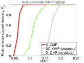
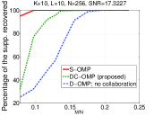
Figure 1: Performance of the sparsity pattern recovery with distributed OMP algorithm: (left) the probability of correctly recovering the sparse support ($P_{D}=Pr(\hat{\mathbf{b}}=\mathbf{b})$) vs $M/N$ (right) the percentage of the support correctly recovered vs $M/N$; $N=256$, $K=10$, $L=10$, $\bar{\gamma}=\frac{||\mathbf{s}||_{2}^{2}}{N\sigma_{v}^{2}}=17.3227dB$

IV-1 Updating $i_{index}$ in step 4

Step 4 in Algorithm 2 is performed as given below. At $t$-th iteration, $c_{l}(t)$ contains all the indices received by the $l$-th node from its neighborhood. The function $unique(c_{l}(t))$ gives the number of distinct indices of the support set in $c(t)$. If all the indices in $c_{l}(t)$ are different from each other, $unique(c_{l}(t))$ equals to the number of nodes in the neighborhood of the $l$-th node including itself. If there are any two indices in $c_{l}(t)$ with the same value, we set the value of $\rho(c_{l}(t))$ as the number of such indices. After performing $K_{0}$ (which is less than $K$) number of iterations, if $i_{index}$ in step 4 in Algorithm 2 is very small (less than $I_{0}$ where $I_{0}\ll K$), the algorithm decides that no sparse signal is present and terminate the process resulting in the null set as the estimated support set. If $i_{index}\geq I_{0}$, it decides that the sparse signal is present and continues estimating the support set similar to Algorithm 1.

V Simulation Results

In this section, we present some simulation results to demonstrate the performance of proposed algorithms for sparsity pattern recovery based on distributed CS based measurements. In the following, we assume that the entries of each projection matrix $\mathbf{A}_{l}$ for $l=0,1,\cdots,L-1$ are drawn from a Gaussian ensemble with mean zero and variance $\frac{1}{N}$.

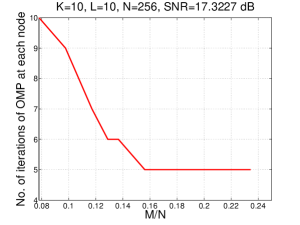
Figure 2: Number of iterations of OMP at each node with the proposed Algorithm 1 vs $M/N$; $N=256$, $K=10$, $L=10$, $\bar{\gamma}=\frac{||\mathbf{s}||_{2}^{2}}{N\sigma_{v}^{2}}=17.3227dB$,

To compare the performance of the proposed Algorithm 1 with other approaches, we consider two benchmark cases. (i). Distributed OMP with no collaboration: in this case, each node performs OMP independently to obtain the support set estimate $\hat{\mathcal{U}}_{l}(t)$, i.e., the step 3 is eliminated in Algorithm 1 and set $\lambda_{l}^{*}(t)=\lambda_{l}(t)$. To fuse the support sets estimated at individual nodes, each node transmits its estimated support to a fusion center and performs a majority rule based fusion scheme to obtain a global estimate of $\mathcal{U}$. (ii). Simultaneous OMP (S-OMP) [32]: S-OMP algorithm is carried out using all the raw observations at the fusion center. Thus, this scheme requires each node to transmit its $M$-length observation vector as well as the projection matrix $\mathbf{A}_{l}$ to the fusion center.

In Figures 1 and 2, we illustrate the performance of the sparsity pattern estimation based on proposed DC-OMP as in Algorithm 1 in terms of different performance metrics. In both figures, we let $K=10$, $N=256$, $L=10$, and SNR at each node, defined as $\bar{\gamma}=\frac{||\mathbf{s}||_{2}^{2}}{N\sigma_{v}^{2}}=17.3227dB$. Also, in Figures 1 and 2 we assume that $\mathcal{M}_{l}=\bar{\mathcal{M}}$ as considered in case I in Subsection III-1. Then the estimated support set at each node based on Algorithm 1 is the same. In Fig. 1, by performing $10^{4}$ runs and averaging over 10 trials, we plot the probability of correctly recovering the full support set, $P_{D}=Pr(\hat{\mathbf{b}}=\mathbf{b})$ (left) and the percentage of the support set that is estimated correctly (right) vs $M/N$ where $M$ is the number of compressive measurements at each node. It can be seen from Fig. 1 that, at relatively small values of $M/N$, the proposed algorithm outperforms D-OMP with no collaboration. In resource constrained distributed networks, especially in sensor networks, it is desirable to perform the desired task by employing less measurement data (i.e. with small $M$) at each node distributing the computational complexity among nodes to save the overall node power. Thus, fusing the estimated indices of the non-zero coefficients at each iteration of the OMP algorithm ensures a higher performance in exact sparsity pattern recovery compared to that when OMP is performed at each node independently. However, as $M/N$ increases, $Pr(\hat{\mathbf{b}}=\mathbf{b})$ of both algorithms converge to 1, since when the number of compressive measurement at each node increases, OMP (with or without collaboration) works better and recovers the sparsity pattern almost exactly with a single measurement vector. It has been shown in [8, 37] that OMP requires approximately $M\geq(1+\epsilon)4K\log N$, $\epsilon>0$ measurements for reliable sparsity pattern recovery in the noise free case. Thus, even with a very small $M$ at each node, having $L$ number of nodes, S-OMP achieves this limit and provides a significant performance gain compared to the proposed algorithm at very small $M/N$ values. However, S-OMP requires a considerable communication overhead compared to the proposed algorithm. Further, in the proposed algorithm, each node has the same estimator at the end in contrast to the centralized S-OMP.

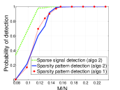
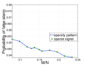
Figure 3: Performance of the sparse signal detection and sparsity pattern recovery with Algorithm 2; $N=256$, $K=10$, $L=10$, $\bar{\gamma}=\frac{||\mathbf{s}||_{2}^{2}}{N\sigma_{v}^{2}}=17.3227dB$; (left) Probability of detection, (right) probability of false alarms

In Fig. 1, we further plot the percentage of support that is correctly recovered. for example, at $\frac{M}{N}\approx 0.1$, the proposed algorithm correctly recovers approximately $75\%$ of the support while D-OMP with no collaboration recovers only about $30\%$ of the support. Thus, from both sub figures of Fig. 1, significant performance gain is observed via the proposed algorithm compared to D-OMP with no collaboration with small $M$, which is the more desirable scenario in resource constrained distributed networks. To further illustrate the efficiency of the proposed algorithm, in Fig. 2, we plot the number of iterations of the DC-OMP algorithm that each node has to perform in recovering the sparsity pattern. It is observed from Fig. 2 that as $M/N$ increases, the proposed algorithm estimates the sparsity pattern reliably by executing only $\approx K/2$ number of iterations at each node. When $M/N$ increases, as observed from Fig. 1, the performance of both DC-OMP and D-OMP with no collaboration converges to the same level but DC-OMP requires very small number of iterations at each node to achieve that performance compared to that with D-OMP with no collaboration which requires $K$ number of iterations at each node irrespective of the value of $M/N$.

In Fig. 3, we illustrate the performance of Algorithm 2 for detecting the sparse signal before estimating the sparsity pattern. We plot the performance of sparse signal detection as well as the sparsity pattern estimation in Fig. 3. For sparse signal detection, probability of detection and the false alarm are given by $P_{D}^{s}=Prob(\delta=1|\mathcal{H}_{1})$ and $P_{F}^{s}=Prob(\delta=1|\mathcal{H}_{0})$, respectively where $\delta$ is the detection decision. For sparsity pattern detection, the probability of detection is given by $P_{D}^{u}=Prob(\hat{\mathbf{b}}=\mathbf{b}^{1}|\mathcal{H}_{1})Prob(\mathcal{H}_{1})+Prob(\hat{\mathbf{b}}=\mathbf{b}^{0}|\mathcal{H}_{0})Prob(\mathcal{H}_{0})$, where we redefine the variables such that $\mathbf{b}^{1}$ is the binary support of the signal $\mathbf{s}$ (i.e. the support under $\mathcal{H}_{1}$) while $\mathbf{b}^{0}$ denotes the vector with all zeros (binary support under $\mathcal{H}_{0}$). Similarly the probability of false alarm, is given by $P_{F}^{u}=Prob(\hat{\mathbf{b}}=\mathbf{b}^{1}|\mathcal{H}_{0})Prob(\mathcal{H}_{1})+Prob(\hat{\mathbf{b}}=\mathbf{b}^{0}|\mathcal{H}_{1})Prob(\mathcal{H}_{0})$. Further, in Fig. 3 we use the same values for the parameters $N,K,L$ and $\bar{\gamma}$ as used in Figures 1 and 2 and $K_{0}=3$ and $I_{0}=2$. From Fig. 3, it is seen that Algorithm 2 reliably detects the sparse signal even with a very small value of $M/N$, and the performance of the sparsity pattern recovery after detecting the signal has performance that is close to that when the sparsity pattern recovery is done as in Algorithm 1 (where it is known a priori that the signal is present).

VI conclusion

In this paper, we addressed the problem of recovering a common sparsity pattern based on CS measurement vectors collected at distributed nodes in a distributed network. A distributed greedy algorithm based on OMP is proposed to estimate the sparsity pattern via collaboration in which each distributed node is required to perform less number of iterations of the greedy algorithm compared to the sparsity index. When it is not known a priori that a sparse signal is present or not, the algorithm was extended to perform detection of the sparse signal with a fewer number of iterations before completely recovering the sparsity pattern. The proposed algorithm is shown to have significant performance gains compared to that with each node performing OMP independently and then fusing the estimated supports to achieve a global estimate. Complete theoretical analysis of the algorithm will be considered in a future work.

References

- [1] D. Donoho, “Compressed sensing,” IEEE Trans. Inform. Theory, vol. 52, no. 4, pp. 1289–1306, Apr. 2006.
- [2] E. Cands and M. B. Wakin, “An introduction to compressive sampling,” IEEE Signal Processing Magazine, pp. 21–30, Mar. 2008.
- [3] R. G. Baraniuk, “Compressive sensing,” IEEE Signal Processing Magazine, pp. 118–120, 124, Jul. 2008.
- [4] E. Cands and J. Romberg, “Practical signal recovery from random projections,” Preprint, Jan. 2004.
- [5] E. Cands, J. Romberg, and T. Tao, “Stable signal recovery from incomplete and inaccurate measurements,” Communications on Pure and Applied Mathematics, vol. 59, no. 8, pp. 1207–1223, Aug. 2006.
- [6] J. K. Romberg, “Sparse signal recovery via l1 minimization,” in 40th Annual Conf. on Information Sciences and Systems (CISS), Princeton, NJ, Mar. 2006, pp. 213–215.
- [7] J. N. Laska, M. A. Davenport, and R. G.Baraniuk, “Exact signal recovery from sparsely corrupted measurements through the pursuit of justice,” in Asilomar Conference on Signals, Systems, and Computers, Pacific Grove, California, Nov. 2009, pp. 1556–1560.
- [8] J. Tropp and A. Gilbert, “Signal recovery from random measurements via orthogonal matching pursuit,” IEEE Trans. Inform. Theory, vol. 53, no. 12, pp. 4655–4666, Dec. 2007.
- [9] M. A. T. Figueiredo, R. D. Nowak, and S. J. Wright, “Gradient projection for sparse reconstruction: Application to compressed sensing and other inverse problems,” IEEE Journal of Selected Topics in Signal Processing: Special Issue on Convex Optimization Methods for Signal Processing, vol. 1, no. 4, 2007.
- [10] T. Blumensath and M. E. Davies, “Iterative thresholding for sparse approximations,” Preprint, 2007.
- [11] ——, “Gradient pursuits,” IEEE Trans. Signal Processing, vol. 56, no. 6, pp. 2370–2382, June 2008.
- [12] D. Needell and R. Vershynin, “Uniform uncertainty principle and signal recovery via regularized orthogonal matching pursuit,” Preprint, 2007.
- [13] D. Malioutov, M. Cetin, and A.Willsky, “A sparse signal reconstruction perspective for source localization with sensor arrays,” IEEE Trans. Signal Processing, vol. 53, no. 8, pp. 3010–3022, Aug. 2005.
- [14] V. Cevher, P. Indyk, C. Hegde, and R. G. Baraniuk, “Recovery of clustered sparse signals from compressive measurements,” in Int. Conf. Sampling Theory and Applications (SAMPTA 2009), Marseille, France, May. 2009, pp. 18–22.
- [15] Z. Tian and G. Giannakis, “Compressed sensing for wideband cognitive radios,” in Proc. Acoust., Speech, Signal Processing (ICASSP), Honolulu, HI, Apr. 2007, pp. IV–1357–IV–1360.
- [16] Y. Jin, Y.-H. Kim, and B. D. Rao, “Support recovery of sparse signals,” arXiv:1003.0888v1[cs.IT], 2010.
- [17] S. Baillet, J. C. Mosher, and R. M. Leahy, “Electromagnetic brain mapping,” IEEE Signal Process. Mag., pp. 14–30, 2001.
- [18] D. Wipf and S. Nagarajan, “A unified bayesian framework for meg/eeg source imaging,” NeuroImage, pp. 947–966, 2008.
- [19] B. K. Natarajan, “Sparse approximate solutions to linear systems,” SIAM J. Computing, vol. 24, no. 2, pp. 227–234, 1995.
- [20] A. J. Miller, Subset Selection in Regression. New York, NY: Chapman-Hall, 1990.
- [21] E. G. Larsson and Y. Sel n, “Linear regression with a sparse parameter vector,” IEEE Trans. Signal Processing, vol. 55, no. 2, pp. 451–460, Feb.. 2007.
- [22] S. S. Chen, D. L. Donoho, and M. A. Saunders, “Atomic decomposition by basis pursuit,” SIAM J. Sci. Computing, vol. 20, no. 1, pp. 33–61, 1998.
- [23] M. J. Wainwright, “Information-theoretic limits on sparsity recovery in the high-dimensional and noisy setting,” Univ. of California, Berkeley, Dept. of Statistics, Tech. Rep, Jan. 2007.
- [24] ——, “Information-theoretic limits on sparsity recovery in the high-dimensional and noisy setting,” IEEE Trans. Inform. Theory, vol. 55, no. 12, pp. 5728–5741, Dec. 2009.
- [25] W. Wang, M. J. Wainwright, and K. Ramachandran, “Information-theoretic limits on sparse signal recovery: Dense versus sparse measurement matrices,” IEEE Trans. Inform. Theory, vol. 56, no. 6, pp. 2967–2979, Jun. 2010.
- [26] A. K. Fletcher, S. Rangan, and V. K. Goyal, “Necessary and sufficient conditions for sparsity pattern recovery,” IEEE Trans. Inform. Theory, vol. 55, no. 12, pp. 5758–5772, Dec. 2009.
- [27] M. M. Akcakaya and V. Tarokh, “Shannon-theoretic limits on noisy compressive sampling,” IEEE Trans. Inform. Theory, vol. 56, no. 1, pp. 492–504, Jan. 2010.
- [28] G. Reeves and M. Gastpar, “Sampling bounds for sparse support recovery in the presence of noise,” in IEEE Int. Symp. on Information Theory (ISIT), Toronto, ON, Jul. 2008, pp. 2187–2191.
- [29] G. Tang and A. Nehorai, “Performance analysis for sparse support recovery,” IEEE Trans. Inform. Theory, To appear 2010.
- [30] V. K. G. A. K. Fletcher and S. Rangan, “Compressive sampling and lossy compression,” IEEE Signal Processing Magazine, vol. 25, no. 2, pp. 48–56, Mar. 2008.
- [31] T. Wimalajeewa and P. K. Varshney, “Performance bounds for sparsity pattern recovery with quantized noisy random projections,” IEEE Journal of Selected Topics in Signal Processing, Special Issue on Robust Measures and Tests Using Sparse Data for Detection and Estimation, vol. 6, no. 1, pp. 43 – 57, Feb. 2012.
- [32] J. A. Tropp, A. C. Gilbert, and M. J. Strauss, “Simultaneous sparse approximation via greedy pursuit,” in Proc. Acoust., Speech, Signal Processing (ICASSP), 2005, pp. V–721–V–724.
- [33] S. S. M. B. W. D. Baron, M. Duarte and R. G. Baraniuk, “Distributed compressed sensing,” preprint, 2009.
- [34] Q. Ling and Z. Tian, “Decentralized support detection of multiple measurement vectors with joint sparsity,” in Proc. Acoust., Speech, Signal Processing (ICASSP), 2011, pp. 2996–2999.
- [35] F. Zeng, C. Li, and Z. Tian, “Distributed compressive spectrum sensing in cooperative multihop cognitive networks,” IEEE Journal of Selected Topics in Signal Processing, vol. 5, no. 1, pp. 37–48, Feb. 2011.
- [36] R. Tibshirani, “Regression shrinkage and selection via the lasso,” J. Royal Statist. Soc B, vol. 58, no. 1, pp. 267–288, 1996.
- [37] A. Fletcher and S. Rangan, “Orthogonal matching pursuit from noisy random measurements: A new analysis,” in NIPS’09, 2009.